6281441-thesis

Real-Time Traffic Sign Detection

using Hierarchical Distance Matching

by

Craig Northway

A thesis submitted to the

School of Information Technology and Electrical Engineering

The University of Queensland

for the degree of

BACHELOR OF ENGINEERING

October 2002

Statement of originality

I declare that the work presented in the thesis is, to the best of my knowledge and belief, origi-

nal and my own work, except as acknowledged in the text, and that the material has not been

submitted, either in whole or in part, for a degree at this or any other university.

Craig Northway

iii

Acknowledgments

There are many people who deserve acknowledgment for the help I have received while working

on this thesis and during my 16 years of study. Unfortunately its impossible to mention them

all!

From an academic perspective I must thank my supervisor Brian Lovell for his technical help

when I was struggling, excellent view of the big picture and promotion of my work. Shane

Goodwin deserves mention for his help as the lab supervisor organising cameras and facilities.

The excellent background Vaughan Clarkson’s course, ELEC3600, gave me in this area was

invaluable.

I’d like to thank all of my friends and family, particularly my girlfriend and best friend, Sarah

Adsett and my parents Bruce and Rosalie Northway for their support. To my ”non-engineering”

friends Michael, Jesse and Jon, thanks, now its handed in you can contact me again.

To all the engineers: Hope you enjoyed your degree as much as I have! Special thanks goes to

Nia, for the use of her laptop. To Jenna and Ben Appleton and Simon Long for their signals

related technical insights. I’ll also single out Toby, Vivien, Scott, Leon and the rest of the SEES

exec.

“Get Naked for SEES 2002!”

v

Abstract

Smart Cars that avoid pedestrians, and remind you of the speed limits? Vehicles will soon have

the ability to warn drivers of pending situations or automatically take evasive action. Due to

the visual nature of existing infrastructure, signs and line markings, image processing will play a

large part in these systems. This thesis will develop a real-time traffic sign detection algorithm

using hierarchical distance matching.

There are four deliverables for the thesis:

1. A hierarchy creation system built in MATLAB

2. A prototype Matching system also built in MATLAB

3. A real-time application in Visual C++ using the DirectShow SDK and IPL Image Pro-

cessing and OpenCV libraries.

4. Examples of other uses for the matching algorithm.

The hierarchy creation system is based on simple graph theory and creates small (< 50) hi-

erarchies of templates. The prototype matching system uses static images and was designed

to explore the matching algorithm. Matching of up to 20 frames per second using a 30+ leaf

hierarchy was achieved in the real-time with a few false matches.

Other matching examples demonstrated include “Letter” matching, rotational and scale invari-

ant matching. Future work on this thesis would include the development of a final verification

stage to eliminate the false matches. Refactoring of the systems design would also allow for

larger hierarchies to be created and searched, increasing the robustness and applications of the

algorithm.

vii

Contents

Statement of originality iii

Acknowledgments v

Abstract vii

1 Introduction 1

2 Topic 3

2.1 Extensions . . . . . . . . . . . . . . . . . . . . . . . . . . . . . . . . . . . . . . . . 4

2.2 Deliverables . . . . . . . . . . . . . . . . . . . . . . . . . . . . . . . . . . . . . . . 4

3 Assumptions 5

4 Specification 7

4.1 MATLAB Hierarchy Creation . . . . . . . . . . . . . . . . . . . . . . . . . . . . . 7

4.2 MATLAB Matching Prototype . . . . . . . . . . . . . . . . . . . . . . . . . . . . 8

4.3 Real-Time Implementation . . . . . . . . . . . . . . . . . . . . . . . . . . . . . . 8

4.4 Smart Vehicle System . . . . . . . . . . . . . . . . . . . . . . . . . . . . . . . . . 8

ix

x CONTENTS

5 Literature Review 11

5.1 Historical Work: Chamfer Matching . . . . . . . . . . . . . . . . . . . . . . . . . 11

5.2 Current Matching Algorithms . . . . . . . . . . . . . . . . . . . . . . . . . . . . . 12

5.2.1 Current Hierarchical Distance Matching Applications . . . . . . . . . . . 12

5.2.2 Other Possible Techniques . . . . . . . . . . . . . . . . . . . . . . . . . . . 14

5.3 Hierarchies and Trees . . . . . . . . . . . . . . . . . . . . . . . . . . . . . . . . . 15

5.3.1 Graph Theoretic Approach . . . . . . . . . . . . . . . . . . . . . . . . . . 16

5.3.2 Nearest Neighbour . . . . . . . . . . . . . . . . . . . . . . . . . . . . . . . 17

5.3.3 Colour Information . . . . . . . . . . . . . . . . . . . . . . . . . . . . . . . 17

6 Theory 19

6.1 Chamfer Matching . . . . . . . . . . . . . . . . . . . . . . . . . . . . . . . . . . . 19

6.2 Feature Extraction . . . . . . . . . . . . . . . . . . . . . . . . . . . . . . . . . . . 20

6.2.1 Edge detection . . . . . . . . . . . . . . . . . . . . . . . . . . . . . . . . . 20

6.3 Distance Transform . . . . . . . . . . . . . . . . . . . . . . . . . . . . . . . . . . . 22

6.4 Distance Matching . . . . . . . . . . . . . . . . . . . . . . . . . . . . . . . . . . . 23

6.4.1 Reverse Matching . . . . . . . . . . . . . . . . . . . . . . . . . . . . . . . 25

6.4.2 Oriented Edge Matching . . . . . . . . . . . . . . . . . . . . . . . . . . . . 26

6.4.3 Coarse/Fine Search . . . . . . . . . . . . . . . . . . . . . . . . . . . . . . 26

6.4.4 Hierarchy Search . . . . . . . . . . . . . . . . . . . . . . . . . . . . . . . . 27

6.5 Tree/Hierarchy . . . . . . . . . . . . . . . . . . . . . . . . . . . . . . . . . . . . . 28

6.5.1 Graph Theory . . . . . . . . . . . . . . . . . . . . . . . . . . . . . . . . . 28

CONTENTS xi

6.5.2 Trees . . . . . . . . . . . . . . . . . . . . . . . . . . . . . . . . . . . . . . . 29

6.6 Programming . . . . . . . . . . . . . . . . . . . . . . . . . . . . . . . . . . . . . . 33

7 Hardware Design and Implementation 35

7.1 Camera . . . . . . . . . . . . . . . . . . . . . . . . . . . . . . . . . . . . . . . . . 36

8 Software Design and Implementation 37

8.1 Hierarchy Creation . . . . . . . . . . . . . . . . . . . . . . . . . . . . . . . . . . . 37

8.1.1 Image Acquisition . . . . . . . . . . . . . . . . . . . . . . . . . . . . . . . 38

8.2 Group Creation . . . . . . . . . . . . . . . . . . . . . . . . . . . . . . . . . . . . . 40

8.2.1 Finding groups - setup.m . . . . . . . . . . . . . . . . . . . . . . . . . . . 41

8.2.2 Score Calculation - createtemps.m . . . . . . . . . . . . . . . . . . . . . . 42

8.2.3 Hierarchy Creation . . . . . . . . . . . . . . . . . . . . . . . . . . . . . . . 43

8.2.4 Hierarchy Optimisation . . . . . . . . . . . . . . . . . . . . . . . . . . . . 44

8.2.5 Multi-Level Hierarchy . . . . . . . . . . . . . . . . . . . . . . . . . . . . . 45

8.2.6 Final Implementation . . . . . . . . . . . . . . . . . . . . . . . . . . . . . 46

8.3 MATLAB Prototype Matching . . . . . . . . . . . . . . . . . . . . . . . . . . . . 46

8.3.1 Basic System . . . . . . . . . . . . . . . . . . . . . . . . . . . . . . . . . . 47

8.3.2 Masking Reverse Search . . . . . . . . . . . . . . . . . . . . . . . . . . . . 48

8.3.3 Pyramid Search . . . . . . . . . . . . . . . . . . . . . . . . . . . . . . . . . 49

8.3.4 Directional Matching . . . . . . . . . . . . . . . . . . . . . . . . . . . . . . 52

8.3.5 Rejected Refinements . . . . . . . . . . . . . . . . . . . . . . . . . . . . . 55

8.3.6 Final Implementation . . . . . . . . . . . . . . . . . . . . . . . . . . . . . 55

xii CONTENTS

8.4 Real-Time . . . . . . . . . . . . . . . . . . . . . . . . . . . . . . . . . . . . . . . . 56

8.4.1 Matching Process . . . . . . . . . . . . . . . . . . . . . . . . . . . . . . . . 56

8.4.2 Object Oriented Design . . . . . . . . . . . . . . . . . . . . . . . . . . . . 56

8.4.3 Actual Design . . . . . . . . . . . . . . . . . . . . . . . . . . . . . . . . . . 58

8.4.4 Further Information . . . . . . . . . . . . . . . . . . . . . . . . . . . . . . 59

8.4.5 Enhancements/Refinements . . . . . . . . . . . . . . . . . . . . . . . . . . 59

8.4.6 Final Matching Algorithm Used. . . . . . . . . . . . . . . . . . . . . . . . 60

8.4.7 Further Examples . . . . . . . . . . . . . . . . . . . . . . . . . . . . . . . 60

9 Results 63

9.1 Hierarchy Creation . . . . . . . . . . . . . . . . . . . . . . . . . . . . . . . . . . . 63

9.1.1 Hierarchies . . . . . . . . . . . . . . . . . . . . . . . . . . . . . . . . . . . 63

9.2 Matlab Matching . . . . . . . . . . . . . . . . . . . . . . . . . . . . . . . . . . . . 65

9.2.1 Matlab Matching Results . . . . . . . . . . . . . . . . . . . . . . . . . . . 65

9.3 Real-Time Matching . . . . . . . . . . . . . . . . . . . . . . . . . . . . . . . . . . 65

9.3.1 Performance . . . . . . . . . . . . . . . . . . . . . . . . . . . . . . . . . . 66

9.3.2 Results . . . . . . . . . . . . . . . . . . . . . . . . . . . . . . . . . . . . . 66

9.3.3 Letter Matching . . . . . . . . . . . . . . . . . . . . . . . . . . . . . . . . 67

9.3.4 Size Variant Matching . . . . . . . . . . . . . . . . . . . . . . . . . . . . . 67

9.3.5 Rotational Matching . . . . . . . . . . . . . . . . . . . . . . . . . . . . . . 67

9.4 My Performance . . . . . . . . . . . . . . . . . . . . . . . . . . . . . . . . . . . . 68

9.4.1 Skills Learnt . . . . . . . . . . . . . . . . . . . . . . . . . . . . . . . . . . 68

9.4.2 Strengths/Weaknesses . . . . . . . . . . . . . . . . . . . . . . . . . . . . . 68

CONTENTS xiii

10 Future Development 69

10.1 Video Footage . . . . . . . . . . . . . . . . . . . . . . . . . . . . . . . . . . . . . . 69

10.2 Temporal Information . . . . . . . . . . . . . . . . . . . . . . . . . . . . . . . . . 70

10.3 Better OO Design . . . . . . . . . . . . . . . . . . . . . . . . . . . . . . . . . . . 70

10.4 Improved Hierarchy Generation . . . . . . . . . . . . . . . . . . . . . . . . . . . . 70

10.5 Optimisation . . . . . . . . . . . . . . . . . . . . . . . . . . . . . . . . . . . . . . 70

10.6 Final Verification Stage . . . . . . . . . . . . . . . . . . . . . . . . . . . . . . . . 70

11 Conclusions 71

12 Publication 73

12.1 Australia’s Innovators Of The Future . . . . . . . . . . . . . . . . . . . . . . . . . 73

A 79

A.1 Assumptions . . . . . . . . . . . . . . . . . . . . . . . . . . . . . . . . . . . . . . 79

A.1.1 Speed . . . . . . . . . . . . . . . . . . . . . . . . . . . . . . . . . . . . . . 79

A.1.2 Lighting . . . . . . . . . . . . . . . . . . . . . . . . . . . . . . . . . . . . . 79

A.1.3 Position . . . . . . . . . . . . . . . . . . . . . . . . . . . . . . . . . . . . . 79

A.1.4 Angle . . . . . . . . . . . . . . . . . . . . . . . . . . . . . . . . . . . . . . 80

A.1.5 Damage . . . . . . . . . . . . . . . . . . . . . . . . . . . . . . . . . . . . . 80

A.1.6 Size . . . . . . . . . . . . . . . . . . . . . . . . . . . . . . . . . . . . . . . 80

A.1.7 Computer Vision Functions . . . . . . . . . . . . . . . . . . . . . . . . . . 81

A.1.8 Objects . . . . . . . . . . . . . . . . . . . . . . . . . . . . . . . . . . . . . 81

A.2 Programming . . . . . . . . . . . . . . . . . . . . . . . . . . . . . . . . . . . . . . 82

xiv CONTENTS

A.2.1 MATLAB . . . . . . . . . . . . . . . . . . . . . . . . . . . . . . . . . . . . 82

A.2.2 Direct Show . . . . . . . . . . . . . . . . . . . . . . . . . . . . . . . . . . . 82

A.2.3 IPL Image Processing Library . . . . . . . . . . . . . . . . . . . . . . . . . 82

A.2.4 Open CV . . . . . . . . . . . . . . . . . . . . . . . . . . . . . . . . . . . . 82

A.3 Extra Hierarchy Implementation Flowcharts . . . . . . . . . . . . . . . . . . . . . 84

A.4 Prototype Orientation Code . . . . . . . . . . . . . . . . . . . . . . . . . . . . . . 87

A.4.1 Orientated Edge Transform . . . . . . . . . . . . . . . . . . . . . . . . . . 87

A.4.2 Orientation Map . . . . . . . . . . . . . . . . . . . . . . . . . . . . . . . . 87

A.5 Rejected Prototype Implementations . . . . . . . . . . . . . . . . . . . . . . . . . 89

A.5.1 Localised Tresholding . . . . . . . . . . . . . . . . . . . . . . . . . . . . . 89

A.5.2 Different Feature Extractions . . . . . . . . . . . . . . . . . . . . . . . . . 91

A.5.3 Sub-Sampling . . . . . . . . . . . . . . . . . . . . . . . . . . . . . . . . . . 91

A.6 UML of Real-Time System . . . . . . . . . . . . . . . . . . . . . . . . . . . . . . 92

A.7 Code Details of Real-Time System . . . . . . . . . . . . . . . . . . . . . . . . . . 95

A.7.1 Distance Transform . . . . . . . . . . . . . . . . . . . . . . . . . . . . . . 95

A.7.2 Deallocation . . . . . . . . . . . . . . . . . . . . . . . . . . . . . . . . . . 95

A.7.3 mytree . . . . . . . . . . . . . . . . . . . . . . . . . . . . . . . . . . . . . . 96

A.7.4 Template Format . . . . . . . . . . . . . . . . . . . . . . . . . . . . . . . . 97

A.8 Tested Enhancements/Refinements to Real-Time System . . . . . . . . . . . . . . 98

A.9 Hierarchy Results . . . . . . . . . . . . . . . . . . . . . . . . . . . . . . . . . . . . 102

A.9.1 Diamond Signs . . . . . . . . . . . . . . . . . . . . . . . . . . . . . . . . . 102

A.9.2 Circular Signs Scores . . . . . . . . . . . . . . . . . . . . . . . . . . . . . . 111

CONTENTS xv

A.10 Matlab Matching Results . . . . . . . . . . . . . . . . . . . . . . . . . . . . . . . 112

A.11 CD . . . . . . . . . . . . . . . . . . . . . . . . . . . . . . . . . . . . . . . . . . . . 115

A.12 Code . . . . . . . . . . . . . . . . . . . . . . . . . . . . . . . . . . . . . . . . . . . 115

A.12.1 Listing . . . . . . . . . . . . . . . . . . . . . . . . . . . . . . . . . . . . . . 115

A.12.2 Compilation . . . . . . . . . . . . . . . . . . . . . . . . . . . . . . . . . . . 117

xvi CONTENTS

List of Figures

1.1 System Output . . . . . . . . . . . . . . . . . . . . . . . . . . . . . . . . . . . . . 1

3.1 Likely Sign Position . . . . . . . . . . . . . . . . . . . . . . . . . . . . . . . . . . 6

4.1 Real Time Traffic Sign System . . . . . . . . . . . . . . . . . . . . . . . . . . . . 9

5.1 Binary Target Hierarchy [1] . . . . . . . . . . . . . . . . . . . . . . . . . . . . . . 14

5.2 Image Clustering with Graph Theory [2] . . . . . . . . . . . . . . . . . . . . . . . 16

6.1 Canny Edge Detection Process . . . . . . . . . . . . . . . . . . . . . . . . . . . . 21

6.2 3-4 Distance Transform (not divided by 3) . . . . . . . . . . . . . . . . . . . . . . 23

6.3 Overlaying of Edge Image [3] . . . . . . . . . . . . . . . . . . . . . . . . . . . . . 23

6.4 Original Image . . . . . . . . . . . . . . . . . . . . . . . . . . . . . . . . . . . . . 24

6.5 Distance Image . . . . . . . . . . . . . . . . . . . . . . . . . . . . . . . . . . . . . 24

6.6 Template . . . . . . . . . . . . . . . . . . . . . . . . . . . . . . . . . . . . . . . . 24

6.7 Matching Techniques [4] . . . . . . . . . . . . . . . . . . . . . . . . . . . . . . . . 25

6.8 Template Distance Transform . . . . . . . . . . . . . . . . . . . . . . . . . . . . . 25

6.9 Search Expansion . . . . . . . . . . . . . . . . . . . . . . . . . . . . . . . . . . . . 27

xvii

xviii LIST OF FIGURES

6.10 Simple Graph [2] . . . . . . . . . . . . . . . . . . . . . . . . . . . . . . . . . . . . 28

6.11 Tree . . . . . . . . . . . . . . . . . . . . . . . . . . . . . . . . . . . . . . . . . . . 30

6.12 Breadth First Search . . . . . . . . . . . . . . . . . . . . . . . . . . . . . . . . . . 32

7.1 Block Diagram from GraphEdit . . . . . . . . . . . . . . . . . . . . . . . . . . . . 36

8.1 Hierarchy Creation Block Diagram . . . . . . . . . . . . . . . . . . . . . . . . . . 38

8.2 Image Acquisition Flowchart . . . . . . . . . . . . . . . . . . . . . . . . . . . . . 39

8.3 My Chamfer Transform . . . . . . . . . . . . . . . . . . . . . . . . . . . . . . . . 40

8.4 Group Creation Block Diagram . . . . . . . . . . . . . . . . . . . . . . . . . . . . 41

8.5 Hierarchy Creation Flowchart . . . . . . . . . . . . . . . . . . . . . . . . . . . . . 44

8.6 combinegroups.m Flowchart . . . . . . . . . . . . . . . . . . . . . . . . . . . . . . 45

8.7 Simple Matching System . . . . . . . . . . . . . . . . . . . . . . . . . . . . . . . . 47

8.8 Noise Behind Sign . . . . . . . . . . . . . . . . . . . . . . . . . . . . . . . . . . . 48

8.9 Reverse Matching Mask . . . . . . . . . . . . . . . . . . . . . . . . . . . . . . . . 49

8.10 Pyramid Search . . . . . . . . . . . . . . . . . . . . . . . . . . . . . . . . . . . . . 50

8.11 Oriented Edge Detection . . . . . . . . . . . . . . . . . . . . . . . . . . . . . . . . 52

8.12 Orientation Map . . . . . . . . . . . . . . . . . . . . . . . . . . . . . . . . . . . . 53

8.13 Intended Class Diagram . . . . . . . . . . . . . . . . . . . . . . . . . . . . . . . . 57

8.14 My Size Variant Hierarchy . . . . . . . . . . . . . . . . . . . . . . . . . . . . . . . 61

9.1 Circular Sign Hierarchy . . . . . . . . . . . . . . . . . . . . . . . . . . . . . . . . 64

9.2 50 Sign . . . . . . . . . . . . . . . . . . . . . . . . . . . . . . . . . . . . . . . . . 66

9.3 60 Sign . . . . . . . . . . . . . . . . . . . . . . . . . . . . . . . . . . . . . . . . . 67

LIST OF FIGURES xix

A.1 Multi-Resolution Hierarchy [4] . . . . . . . . . . . . . . . . . . . . . . . . . . . . 80

A.2 findbestnotin.m Flowchart . . . . . . . . . . . . . . . . . . . . . . . . . . . . . . . 84

A.3 anneal.m Flowchart . . . . . . . . . . . . . . . . . . . . . . . . . . . . . . . . . . . 85

A.4 remove.m Flowchart . . . . . . . . . . . . . . . . . . . . . . . . . . . . . . . . . . 86

A.5 Simple Image . . . . . . . . . . . . . . . . . . . . . . . . . . . . . . . . . . . . . . 89

A.6 Localised Thesholding . . . . . . . . . . . . . . . . . . . . . . . . . . . . . . . . . 90

A.7 Intended Sequence Diagram . . . . . . . . . . . . . . . . . . . . . . . . . . . . . . 92

A.8 Actual Class Diagram . . . . . . . . . . . . . . . . . . . . . . . . . . . . . . . . . 93

A.9 Actual Sequence Diagram . . . . . . . . . . . . . . . . . . . . . . . . . . . . . . . 94

A.10 Spiral Search Pattern . . . . . . . . . . . . . . . . . . . . . . . . . . . . . . . . . . 98

A.11 Straight Search Pattern . . . . . . . . . . . . . . . . . . . . . . . . . . . . . . . . 98

A.12 Untruncated Distance Transform . . . . . . . . . . . . . . . . . . . . . . . . . . . 100

A.13 Truncated Distance Transform . . . . . . . . . . . . . . . . . . . . . . . . . . . . 100

A.14 Original Scores . . . . . . . . . . . . . . . . . . . . . . . . . . . . . . . . . . . . . 102

A.15 Optimised Scores . . . . . . . . . . . . . . . . . . . . . . . . . . . . . . . . . . . . 103

A.16 First Group . . . . . . . . . . . . . . . . . . . . . . . . . . . . . . . . . . . . . . . 104

A.17 First Group Template . . . . . . . . . . . . . . . . . . . . . . . . . . . . . . . . . 104

A.18 Second Group, template = self . . . . . . . . . . . . . . . . . . . . . . . . . . . . 104

A.19 Third Group, template = self . . . . . . . . . . . . . . . . . . . . . . . . . . . . . 105

A.20 Fourth Group . . . . . . . . . . . . . . . . . . . . . . . . . . . . . . . . . . . . . . 105

A.21 Fourth Group Template . . . . . . . . . . . . . . . . . . . . . . . . . . . . . . . . 105

A.22 Fifth Group . . . . . . . . . . . . . . . . . . . . . . . . . . . . . . . . . . . . . . . 106

xx LIST OF FIGURES

A.23 Fifth Group Template . . . . . . . . . . . . . . . . . . . . . . . . . . . . . . . . . 106

A.24 Sixth Group . . . . . . . . . . . . . . . . . . . . . . . . . . . . . . . . . . . . . . . 106

A.25 Sixth Group Template . . . . . . . . . . . . . . . . . . . . . . . . . . . . . . . . . 107

A.26 Seventh Group . . . . . . . . . . . . . . . . . . . . . . . . . . . . . . . . . . . . . 107

A.27 Seventh Group Template . . . . . . . . . . . . . . . . . . . . . . . . . . . . . . . . 107

A.28 Eigth Group . . . . . . . . . . . . . . . . . . . . . . . . . . . . . . . . . . . . . . . 107

A.29 Eight Group Template . . . . . . . . . . . . . . . . . . . . . . . . . . . . . . . . . 108

A.30 First Template Group . . . . . . . . . . . . . . . . . . . . . . . . . . . . . . . . . 109

A.31 First Template Group Combinational Template . . . . . . . . . . . . . . . . . . . 109

A.32 Second Template Group . . . . . . . . . . . . . . . . . . . . . . . . . . . . . . . . 110

A.33 Second Template Group Combinational Template . . . . . . . . . . . . . . . . . . 110

A.34 Last Template Group . . . . . . . . . . . . . . . . . . . . . . . . . . . . . . . . . 110

A.35 Last Template Group Combinational Template . . . . . . . . . . . . . . . . . . . 110

A.36 Second Level Optimisation . . . . . . . . . . . . . . . . . . . . . . . . . . . . . . . 111

A.37 Original Image . . . . . . . . . . . . . . . . . . . . . . . . . . . . . . . . . . . . . 112

A.38 Oriented Edge Image . . . . . . . . . . . . . . . . . . . . . . . . . . . . . . . . . . 112

A.39 Distance Transform Image . . . . . . . . . . . . . . . . . . . . . . . . . . . . . . . 113

A.40 Scores . . . . . . . . . . . . . . . . . . . . . . . . . . . . . . . . . . . . . . . . . . 114

A.41 Closer View of scores . . . . . . . . . . . . . . . . . . . . . . . . . . . . . . . . . . 114

A.42 Match . . . . . . . . . . . . . . . . . . . . . . . . . . . . . . . . . . . . . . . . . . 114

List of Tables

8.1 Directional Scoring . . . . . . . . . . . . . . . . . . . . . . . . . . . . . . . . . . . 54

A.1 Hierarchy . . . . . . . . . . . . . . . . . . . . . . . . . . . . . . . . . . . . . . . . 115

A.2 MATLAB Matching . . . . . . . . . . . . . . . . . . . . . . . . . . . . . . . . . . 116

A.3 Real-Time . . . . . . . . . . . . . . . . . . . . . . . . . . . . . . . . . . . . . . . . 116

xxi

xxii LIST OF TABLES

Chapter 1

Introduction

This thesis will develop a real-time traffic sign matching application. The system will be useful

for autonomous vehicles and smart cars. After testing the matching on traffic signs, other

implementations shall further demonstrate the effectiveness of the algorithm.

A Traffic Sign Recognition system has the potential to reduce the road toll. By “highlighting”

signs and recording signs that have been past, the system would help keep the driver aware

of the traffic situation. There also exists the possibility for computer control of vehicles and

prompting for pedestrians and hazardous road situations.

Figure 1.1: System Output

1

2 CHAPTER 1. INTRODUCTION

If reliable smart vehicle systems can be established on PC platforms upgrading and producing

cars as smart vehicles would be cheap and practical. The European Union are heavily sponsoring

research into this technology through a smart vehicle initiative with a view to decreasing the

road toll.

Hierarchical Distance Matching could be applied to a range of other object detection problems.

Examples of these include pedestrians, cyclists, motorcyclists, military targets, text of known

font, tools, car models, known local landmarks, etc. These recognition cases could be used in

applications such as autonomous vehicles, vehicle identification and mobile robots.

This thesis will help establish a working knowledge of such systems and demonstrate the sim-

plicity of algorithm development on a PC platform. If the goals of the project can be met the

developed application (C++) and associated utilities (MATLABTM ) will form a general solution

for hierarchy creation and implementation.

Some systems already developed by vehicle manufacturers include a night vision system which

Cadillac have introduced into their “Deville” vehicles. This system projects an image of the road

with obstacles highlighted onto the windscreen. Mercedes-Benz’ Freightliner’s Lane Departure

System uses a video camera to monitor lane changes alerting the driver to lane changes without

the use of indicators, possibly due to driver error or fatigue. Daimler Chrysler have produced a

prototype autonomous vehicle capable of handling many and varied traffic scenarios. It uses a

vision system to detect pedestrians and traffic signs.

Chapter 2

Topic

From the background research into shape based object recognition it was obvious that Gavrila’s

Chamfer methods [4, 5] are superior to other approaches for implementation on a general pur-

pose PC platform.

Other methods used for traffic sign detection have included colour detection[6, 7], colour then

shape [8, 9], simulated annealing[10] and neural networks [11]. None of these have been able to

produce an accurate real-time system. Gavrila’s success is due to the simplicity of his algorithm

and its suitability to standard computation and the SIMD instructions. It involves repeated

simple operations (such as addition, multiplication) on the data set which is efficient when com-

puted in this manner.

Another factor contributing to the speed of the algorithm is the coarse/fine and hierarchical na-

ture allowing significant speed-ups (without sacrificing accuracy) when compared to exhaustive

matching. It can be mathematical shown [4, 5] that this pyramid style search will not miss a

match.

Gavrila’s success defined the topic and prompted further research into hierarchies and distance

matching. The topic for this thesis is Real-time Traffic Sign Matching, using Hierarchical Dis-

tance (Chamfer) Matching.

This thesis intends to prove the hypothesis that multiple object detection, such as traffic signs,

can be successful in real-time using a hierarchy of images. Thus video footage can be searched for

N objects simultaneously without the extensive calculations necessary for an exhaustive search

in real-time on a general purpose platform.

3

4 CHAPTER 2. TOPIC

2.1 Extensions

The extensions to previous work [4, 5] and thus the original contribution presented in this thesis

will be the automated hierarchy creation, the independent development and implementation

of Hierarchical Chamfer Matching (HCM) and the evaluation of HCM as a method for object

detection.

2.2 Deliverables

Based on these goals a MATLABTM based Hierarchy creation implementation, a prototype

static matching implementation in MATLABTM and a real-time HCM Object Detection imple-

mentation will be delivered.

The development of this algorithm will allow hierarchies other than the initially intended Traffic

Sign’s to be used, e.g. pedestrians, alpha-numeric characters, car models (from outline/badge),

hand gestures.

Chapter 3

Assumptions

Before commencement of this project some of the assumptions were identified. These assump-

tions must be reasonable for the thesis to be successful. Many of these assumptions are for the

specific task of traffic sign detection. The following assumptions exist:

• Camera should be of a high enough quality to resolve signs at speed.

• Lighting must be such that the camera can produce a reasonable image.

• Signs should be positioned consistently in the footage.

• Angle of the signs in relation to the car’s positions should not be extreme.

• Signs should not be damaged.

• Due to the size invariance of the method the sign should pass through the specific size(s)

without being obscured.

• The Computer Vision functions should operate as specified.

• Objects being detected must be similar in shape for the hierarchy to be effective.

Further Details of these are in Appendix A.1

5

6 CHAPTER 3. ASSUMPTIONS

Figure 3.1: Likely Sign Position

Chapter 4

Specification

The goals of this project are:

1. Establish an automated method of hierarchy creation that can be generalised to any

database of objects with similar features. This system will initially be based in MAT-

LAB.

2. A prototype matching system for static images also built in MATLAB

3. Program an implementation of this object detection in C++ using the Single-Instruction

Multiple Data (SIMD) instructions created for the Intel range of processors. This imple-

mentation will be the problem of traffic sign recognition.

4. Demonstrate the algorithm on other matching problems.

The following specifies clearly the input and output of each deliverable. A brief specification of

what a Smart Vehicle System may do is included.

4.1 MATLAB Hierarchy Creation

The hierarchy creation system should be able to synthesise an image hierarchy without user

input into the classification. This system should work on image databases of reasonable.

7

8 CHAPTER 4. SPECIFICATION

Input

A directory of images (which share similarity), and a threshold for the similarity.

Output

A hierarchy of images and combinational templates.

4.2 MATLAB Matching Prototype

This system should match traffic signs/objects on still images accurately. It is not required to

meet any time constraints

Input

An image hierarchy, and image to be matched.

Output

The image overlayed with matches.

4.3 Real-Time Implementation

This Real-Time Implementation should match objects at over 5 frames per second in reasonable

circumstances. It will be written in Visual C++ based upon the DirectShow streaming media

architecture, developed using the EZRGB24 example (from Microsoft DirectShow SDK A.2).

The image processing operations will be performed by the IPL Image Processing and Open CV

Libraries.

Input

Image hierarchy and video stream.

Output

Video Stream overlayed with matches.

4.4 Smart Vehicle System

A smart vehicle system for driver aid would be a self contained unit, shown in the block diagram

(Figure 4.1). This unit would attach to the car either at manufacture or by “retro-fitting”. It

4.4. SMART VEHICLE SYSTEM 9

would provide the driver with details via either verbal comments, or a heads-up display (output

block). The system would recognise all common warning and speed signs (real-time detection

Figure 4.1: Real Time Traffic Sign System

block). It would be able to keep track of the current speed limit, allowing the driver to check

their speed between signs.

The system may have higher intelligence allowing it to tailor the hierarchy or matching chances

to the situation, eg. if the car is in a 100km zone, a 30km speed sign would be unlikely.

With the use of radar and other visual clues, the system may be able to control the car. This

would avoid possible collisions and keep within the speed limits.

The system must be careful not to lure the driver into a false sense of security. People should

be wary of the systems ability, particularly in extreme situations, such as storms, snow, etc...

10 CHAPTER 4. SPECIFICATION

Chapter 5

Literature Review

The review of background material for this thesis will cover several topics, all relevant to the

project. Firstly several historically significant papers are reviewed. These papers form the

basis of current matching techniques. Secondly, research into state of the art traffic sign and

shape based object detection applications is reviewed, justifying the choice of Hierarchical Based

Chamfer Matching. Current research into image classification and grouping for search and

retrieval is therefore also applicable to this topic. Basic works on trees and graph theory were

examined briefly, along with several mathematical texts to understand the concepts.

5.1 Historical Work: Chamfer Matching

Background work on HCMA (Hierarchical Chamfer Matching Algorithm) was started in the late

70’s. The topic was revisited in the late 80’s by Gunilla Borgefors [3], an authority on Distance

Matching and Transforms. This is well before HCMA systems would have been practical for fast

static matching, let alone real-time video. The algorithm was investigated again throughout the

mid 90’s when implementations on specific hardware became practical.

The first major work on chamfer matching was the 1977 paper “Parametric Correspondence and

chamfer matching: Two new techniques for image matching” by H.G. Barrow et al. This work

discussed the general concept of chamfer matching. That is minimising the generalised distance

between two sets of edge points. It was initially an algorithm only suitable to fine-matching.

11

12 CHAPTER 5. LITERATURE REVIEW

Borgefors [3] extended this early work to present the idea of using a coarse/fine resolution

search. This solved the major problem of the first proposal, its limitation to fine matching. This

algorithm used a distance transform proposed by its author, the 3-4 DT. The paper demonstrated

the algorithms object detecting effectiveness on images of tools on a plain background. Tools

can be recognised based solely on the outline in this situation hence are perfect for HCM. This

was on static images.

Borgefors also proposed the use of the technique for aerial image registration. This idea was later

presented in [12]. The conclusions reached were that the results were “good, even surprisingly

good. Thus the HCMA is an excellent tool for edge matching, as long as it is used for matching

task with in capability(sic).” [3].

The mid-nineties saw several uses of distance transforms as matching algorithms. Considerable

work done on Hausdorff matching by Huttenlocher and Rucklidge in [13, 14] showed that the

Hausdorff distance could be used as a matching metric between two edge images. Their best

results required at least 20 seconds to compute on a binary image of 360x240 pixels. This was

in 1993, assuming Moore’s Law holds, then in 2002 with only hardware improvements, it should

be possible in well under half a second. Hausdorff matching, as with all distance matching

techniques, requires the image to be overlayed over each template to score each match, this is a

computationally expensive operation.

5.2 Current Matching Algorithms

Current approaches to shape based real-time object detection. These include Hierarchical Cham-

fer Matching, Orientated Pixel Matching and Neural Networks. The most successful work pre-

sented in this area is from Dairu Gavrila and associates at Daimler Chrysler using HCMA.

5.2.1 Current Hierarchical Distance Matching Applications

Daimler-Chrysler Autonomous Vehicle

Hierarchical Chamfer Matching (HCM) is currently being used in automated vehicle systems

at Daimler-Chrysler. The systems for both traffic signs and pedestrian detection are based on

5.2. CURRENT MATCHING ALGORITHMS 13

HCM. The most surprising result of this work is the success of rigid, scale and rotation invariant

template based matching for a deformable contour i.e. pedestrian outlines. This approach may

be unique. They have designed algorithms using the SIMD instruction sets provided by Intel for

their MMX architecture. Their experiments show that the traffic sign detection could be run at

10-15 HZ and the pedestrian detection at 1-5 Hz on a dual processor 450MHz Pentium system.

They go onto prove that distance transforms provide a smoother similarity measure than cor-

relations which “enables the use of various efficient search algorithms to lock onto the correct

solution”. These efficient algorithms are coarse-fine searches and multiple template hierarchies.

As suggested in these papers this matching technique is similar to Hausdorff distance methods.

Worst case measurements of matching templates are then considered to determine minimum

thresholds that “assure [the algorithm].will not miss a solution” in their hierarchies of resolu-

tion/template. The hierarchy creation in this system is not fully automated. Their method

of creating the hierarchy automatically uses a “bottom-up approach and applies a “K-means”-

like algorithm at each level” where K is the desired partition size. The clustering is achieved

by trying various combinations of templates from a random starting point and minimising the

maximum distance between the templates in a group and their chosen prototype.

The optimisation is done with simulated annealing. The disadvantage of their early approaches

was in the one-level tree created. The overall technique proposed by Diamler-Chrysler shows

excellent results and is worthy of further development.

Target Recognition

An Automatic Target recognition system developed by Olson and Huttenlocher [1] uses a hier-

archical search tree. Their matching technique employs “oriented edge” pixels, labelling each

edge pixel with a direction. Translated, rotated and scaled views are incorporated into a hier-

archy. Chamfer measures, though not employed in the matching (Hausdorff matching) are used

to cluster the edge maps into groups of two. A new template for each set of pairs is generated

and the clustering continued until all templates belong to a single hierarchy. This creates a

binary search tree (Figure 5.1). The hierarchy creation presented is a simple approach that may

present good results. There is no mention of the real-time performance of the oriented edge

pixel algorithm. It may not be quick enough for traffic sign recognition.


Figure 5.1: Binary Target Hierarchy [1]

Planar Image Mosaicing

Hierarchical Chamfer Matching has been used successfully for Planar-Image Mosaicing. Dha-

naraks and Covaisaruch [12] used HCMA to “find the best matching position from edge feature

(sic) in multi resolution pyramid”. They chose one image to be the “distance” image and another

to be the “polygon” image. The resolution pyramids are built and matching is carried out by

translating the polygon image across the distance image. The interesting concept used in this

work was the thresholding for taking a match to the next level. If the score was less then the

rejection value (max − (max × percent100 )) the pixel was expanded to more positions in the next

pyramid level for matching. This is an interesting thresholding concept based on the maximum

values rather than absolute.

5.2.2 Other Possible Techniques

Hausdorff Matching

Many researchers have considered Hausdorff matching [13, 14, 15] for object detection. It is a

similar algorithm to chamfer matching, except the distance measure cannot be pre-processed. It

is a valid approach for this application and will be considered as a possible matching strategy.

5.3. HIERARCHIES AND TREES 15

Neural Networks

Work by Daniel Rogahn [11] and papers such as [16] are example of neural network techniques

for traffic sign recognition. I do not have the necessary background knowledge to explore this

properly.

Colour detection

Colour data has been used for matching in scenarios such as face detection [18, 19]. Some

traffic sign detection algorithms use it as a cue [6, 7, 8, 9]. It is an excellent technique for

situations where the colours are constant and illumination can be controlled. Due to most

colour representation schemes not being perceptively true, it is difficult to define exact colours

for matching.

Previous work by myself on traffic sign recognition has attempted to incorporate colour data

into the matching process. The overhead of detecting the colour (even with a look up table) and

the varying illumination made it difficult in this real-time scenario. Yellow diamond warning

signs were quiet easily detectable as present in an image. Their features were not perceptible

accurately from colour data alone.

Signs such as those indicating speed limits have a thin red circle surrounding the details. My

previous results have shown that on compressed video this red circle is destroyed by artifacts.

It was impossible to determine if this circle was red or brown. By including it’s colour in the

detection, many unrelated areas of ground and trees were also highlighted. Thus identification

of signs was not plausible from colour detection alone, though it may still be a useful procedure

for masking areas of interest. It may be more effective in streamed uncompressed video.

5.3 Hierarchies and Trees

The results shown by [4, 5] have been far superior to other research [6, 7, 8, 9, 11, 10, 19, 13, 26]

into real time object identification. Further research was therefore carried out into tree structures

and image grouping and classification. Image classification techniques have been examined in

multimedia retrieval systems [20, 2, 21, 22]. Hierarchies and trees have also been investigated


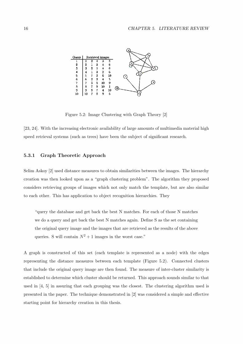
Figure 5.2: Image Clustering with Graph Theory [2]

[23, 24]. With the increasing electronic availability of large amounts of multimedia material high

speed retrieval systems (such as trees) have been the subject of significant research.

5.3.1 Graph Theoretic Approach

Selim Askoy [2] used distance measures to obtain similarities between the images. The hierarchy

creation was then looked upon as a “graph clustering problem”. The algorithm they proposed

considers retrieving groups of images which not only match the template, but are also similar

to each other. This has application to object recognition hierarchies. They

“query the database and get back the best N matches. For each of those N matches

we do a query and get back the best N matches again. Define S as the set containing

the original query image and the images that are retrieved as the results of the above

queries. S will contain N2 + 1 images in the worst case.”

A graph is constructed of this set (each template is represented as a node) with the edges

representing the distance measures between each template (Figure 5.2). Connected clusters

that include the original query image are then found. The measure of inter-cluster similarity is

established to determine which cluster should be returned. This approach sounds similar to that

used in [4, 5] in assuring that each grouping was the closest. The clustering algorithm used is

presented in the paper. The technique demonstrated in [2] was considered a simple and effective

starting point for hierarchy creation in this thesis.

5.3. HIERARCHIES AND TREES 17

5.3.2 Nearest Neighbour

Huang et al [23] used trees established by the nearest neighbour algorithm and built using

normalised cuts (partitions of a weighted graph that minimise the dissociation with other groups

and maximises the association within the group) in a recursive nature. This technique proved

effective in the paper, but was too complicated to pursue in an undergraduate thesis on image

matching.

5.3.3 Colour Information

To group images [20] uses colour information, with a potentially useful clustering technique.

The N images are placed into distinct clusters using their similarity measure. “Two clusters are

picked such that their similarity measure is the largest” these then form a new cluster, reducing

the number of unmerged clusters. The similarity of all the clusters is then computed again.

This continues until a bounding parameter (no. of clusters, or similarity measure threshold) is

reached.

This creates a tree that can at most have two clusters branching off a parent cluster, yet each

leaf cluster could contain more than two images. This allows the simplicity of a binary tree,

with the added complexity of many leaves. To represent each cluster, after the tree has been

created a cluster centre is established. They select a representative image of the cluster rather

than compute a new composite image (first proposed in [23]). Various methods such as linear

regression and boolean features can be used for this. Their method of construction also allows

trees to be created with uneven distances to leaves. This might provide a speed-up in matching

where some images in the hierarchy are relatively unique, providing a short and certain path to

them.

Chapter 6

Theory

The theory behind this thesis is split into 3 main sections. Relevant image processing theories

and techniques are explained first. This is followed by the details of the graph theory and

hierarchy basics necessary to understand and develop this work. Lastly some programming

libraries that may not be familiar to all electrical engineers are mentioned.

Image processing is a relatively dynamic field where many problems are yet to have optimal

solutions, but there are still many basic theories and methods that are accepted as the “way” of

doing things. Some elements of the HCM algorithm use this type of method, but those relating

to the hierarchical search are relatively new to the image processing field.

6.1 Chamfer Matching

The basic idea of Chamfer (or Distance) Matching is to measure the distance between the features

of an image and a template. If this distance measure is below or above a certain threshold it

signifies a match. The steps required are:

1. Feature Extraction

2. Distance Transform

3. Score the template at “all” locations

19

20 CHAPTER 6. THEORY

4. Determine whether the scores indicate a match

In Gavrila’s Hierarchical Chamfer Matching Algorithm (HCMA), distance matching is applied

to the scenario of matching multiple objects. When trying to match a set of images with suf-

ficient similarity, a hierarchical approach can be used. Images can be grouped into a tree and

represented by prototype templates that combine their similar features. By matching with pro-

totypes first a significant speed-up can be observed compared to an exhaustive search for each

template. The following section describes the theory behind each of the steps in simple Distance

Matching, before going onto explain the theory of Gavrila’s HCMA.

6.2 Feature Extraction

Shape based objection recognition starts with feature extraction representations of images.

These features are usually corners and edges. Standard edge and corner detection algorithms

such as Sobel filtering and Canny edge detection can be applied to colour/gray images to gen-

erate binary feature maps.

6.2.1 Edge detection

The goal of edge detection is to produce a “line drawing”. Ideally all edges of objects and changes

in colour should be represented by a single line. There are algorithms that vary from simple to

complex. The generalised form of edge detection is gradient approximation and thresholding.

Of the edge detectors that use gradient approximation there are two types, those that use

first order derivatives and second order derivatives. The boundary of an object is generally a

change in image intensity. Using a first order gradient approximation changes in intensity will

be highlighted, and areas of constant intensity will be ignored. To find changes in intensity we

need to examine the difference between adjacent points.

6.2. FEATURE EXTRACTION 21

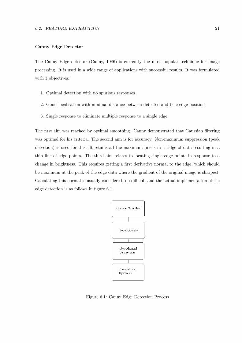
Canny Edge Detector

The Canny Edge detector (Canny, 1986) is currently the most popular technique for image

processing. It is used in a wide range of applications with successful results. It was formulated

with 3 objectives:

1. Optimal detection with no spurious responses

2. Good localisation with minimal distance between detected and true edge position

3. Single response to eliminate multiple response to a single edge

The first aim was reached by optimal smoothing. Canny demonstrated that Gaussian filtering

was optimal for his criteria. The second aim is for accuracy. Non-maximum suppression (peak

detection) is used for this. It retains all the maximum pixels in a ridge of data resulting in a

thin line of edge points. The third aim relates to locating single edge points in response to a

change in brightness. This requires getting a first derivative normal to the edge, which should

be maximum at the peak of the edge data where the gradient of the original image is sharpest.

Calculating this normal is usually considered too difficult and the actual implementation of the

edge detection is as follows in figure 6.1.

Figure 6.1: Canny Edge Detection Process


Non maximal suppression

This essentially locates the highest points in edge magnitude. Given a 3x3 region a point is

considered maximum if its value is greater than those either side of it. The points either side of

it on the edge are established with the direction information.

Hysteresis Thresholding

Hysteresis thresholding allows pixels near edge to be considered as edges for a lower threshold.

If no adjacent pixels are 1 (edge), a high threshold must be met to set a pixel to 1. If there is

an adjacent pixel labelled as 1 a lower threshold must be met to set a pixel to 1.

6.3 Distance Transform

Distance transforms are applied to binary feature images, such as those resulting from edge de-

tection. Each pixel is labelled with a number to represent its distance from the nearest feature

pixel. The real Euclidean distance to pixels is too expensive to calculate and for most applica-

tions an estimate can be used. These include 1-2, 3-4 transforms and other more complicated

approximations. A 3-4 transform uses the following distance operator:

∣∣∣∣∣∣∣∣∣43 1 4

3

1 0 143 1 4

3

∣∣∣∣∣∣∣∣∣ This matrix

shows why the transform is named as such. The diagonals are represented by 43 , and adjacent

distances 33 . Some papers [3, 12, 25] have gone on to prove that approximations were sufficient

for the purposes of distance matching.

The following images show a feature image and its corresponding distance transform. The value

of the distance transform increases as the distance is further from a feature pixel in the original

image. A simple way to calculate a distance transform is to iterate over a feature image using

to distance operator to find the minimum distance value for each pixel. Set all feature pixels

to zero and others to “infinity” before the first pass. Then for each pixel, on each pass, set it

as the following value: vki,j = min(vk−1

i−1,j−1 + 4, vk−1i−1,j + 3, vk−1

i−1,j+1 + 4, vk−1i,j−1 + 3, vk−1

i,j , vk−1i,j+1 +

3, vk−1i+1,j+1 + 4, vk−1

i+1,j + 3, vk−1i+1,j+1 + 4) Complete sufficient passes (k represents the pass number)

6.4. DISTANCE MATCHING 23

∣∣∣∣∣∣∣∣∣∣∣∣∣∣∣∣∣∣

0 0 1 0 1 0

0 0 0 1 0 0

0 0 0 1 0 0

0 0 1 1 0 0

0 0 0 0 0 0

0 0 0 0 0 0

∣∣∣∣∣∣∣∣∣∣∣∣∣∣∣∣∣∣Feature Image

∣∣∣∣∣∣∣∣∣∣∣∣∣∣∣∣∣∣

6 3 0 3 0 3

8 6 3 0 3 6

7 4 3 0 3 6

6 3 0 0 3 6

7 4 3 3 4 7

8 7 6 6 7 8

∣∣∣∣∣∣∣∣∣∣∣∣∣∣∣∣∣∣Distance Transform

Figure 6.2: 3-4 Distance Transform (not divided by 3)

until you have calculated the maximum distance that is necessary for implementation of the

matching or other algorithm you intend to use. More complicated faster methods exist. Borge-

fors is responsible for much of the early work on distance transforms. Her two pass algorithm

[25] is popular and is used by the Open CV library.

6.4 Distance Matching

Distance matching of a single template on an image is a simple process after a feature extraction

and distance transform. One simply scores each position by overlaying the edge data of the

template as shown in figure 6.3. The mean distance of the edge pixels to template is then

Figure 6.3: Overlaying of Edge Image [3]

calculated with Dchamfer(T, I) = 1|T |

∑t∈T dI(t) [5] where T and I are the features of the template

and Image respectively,∣∣∣T ∣∣∣ represents the number of features in T and dI(t) is the distance

between the template and image feature. This gives a matching score. The lower the score, the

better the match. By completing this process for every image position in the region of interest


a score is generated for each location. If any of these scores fall below the matching threshold.

The template can be considered found.

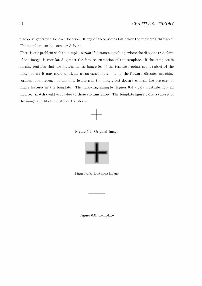
There is one problem with the simple “forward” distance matching, where the distance transform

of the image, is correlated against the feature extraction of the template. If the template is

missing features that are present in the image ie. if the template points are a subset of the

image points it may score as highly as an exact match. Thus the forward distance matching

confirms the presence of template features in the image, but doesn’t confirm the presence of

image features in the template. The following example (figures 6.4 - 6.6) illustrate how an

incorrect match could occur due to these circumstances. The template figure 6.6 is a sub-set of

the image and fits the distance transform.

Figure 6.4: Original Image

Figure 6.5: Distance Image

Figure 6.6: Template


6.4.1 Reverse Matching

A reverse match is often used to preclude these false matches. Figure 6.7 demonstrates the

relationship between a forward match (Feature Template to DT Image) and a reverse match (DT

Template to Feature Image). If we revisit the example that caused errors in forward matching

Figure 6.7: Matching Techniques [4]

we can see that its reverse matching score will be significantly lower. When we combine the

forward and reverse match we can use the resulting score to reject or accept matches. When the

Figure 6.8: Template Distance Transform

template of the cross is overlayed on this distance transform (Figure 6.8) the score will be high.

The only problem is if there are not sufficient pixels in the edge image. This should be eliminated

by forward matching with a “sensible” template.


6.4.2 Oriented Edge Matching

Oriented Edge Matching, and similar techniques, are useful in shape based matching. They

further clarify that features in the template are present in the image. Oriented Edge Matching

can evaluate to a distance measure between orientations. Templates are then matched with this

extra parameter.

Each pixel now has a distance from the nearest feature pixel and an orientation distance from

the nearest feature pixel. Huttenlocher [1] and Johnson [26] have published papers describing

the use of oriented edge matching in an image hierarchy. This orientation match generalised

Hausdorff Matching to oriented pixels. Their formula for calculating the Hausdorff distance took

this extra orientation parameter and normalised it to be comparable with the location distance

measures. Hα(M, I) = maxm∈M (mini∈I(max(

∣∣∣∣∣∣mx− ix

my − iy

∣∣∣∣∣∣ ,

∣∣∣∣mo− io|∣∣∣∣

α ))) [26, 1] Where: m is the

template, mxmy represent the x and y coordinates of that pixel, mo the orientation and similar

for ix, iy, io of the image. It has the same general form as their definition of a Hausdorff measure,

therefore can be substituted into a Hausdorff matching algorithm. Gavrila et al [5] used a similar

technique to increase matching accuracy of chamfer matching.

By splitting the features detected from the extraction into types and matching them separately,

the “chance” that you are measure the distance between the same features of the image and

template increase. Gavrila suggests having M feature types, thus M templates and M feature

images. When using edge points the orientation can be binned into M segments of the unit

circle. Thus each template edge point is assigned to one of the M templates. The individual

distance measures for each M type can be combined later.

6.4.3 Coarse/Fine Search

A Coarse/Fine Search, or pyramid resolution search is a popular method for increasing the speed

of a search based image recognition technique. Generally a coarse fine search involves decreasing

the “steps” of the template search over the image if matching scores dictate.

Conversely a pyramid resolution search scales (smaller) the image and template, increasing the

scale if the scores are sufficient. Though the calculation of the score for each position in a

pyramid search requires less computational expense (less pixels), the scaling of the template can


Figure 6.9: Search Expansion

create difficulties. In a matching scenario such as traffic signs, the details of the signs are quiet

fine. Hence reducing their size can cause these details to be destroyed.

In a distance based search the smooth results (compared to feature to feature matching), mean

that a reasonable match at a coarse search level might indicate an “exact” match at a finer level.

If the current resolution of the search is σ, and the threshold defining a match is θ. Then when

using a distance measure, as in HCM, the current threshold, Tσ, can be set such that a match

“cannot” be missed. Figure 6.9 shows the furthest the actual location (the cross) can be from

the search (squares).

To not miss this possibility the threshold must be set according to: Tσ = θ −√

2 ∗ (σ2 )2. Thus

HCM has the excellent property that in a coarse fine search a “match” cannot be missed.

6.4.4 Hierarchy Search

The approach proposed by Gavrila [4, 5] is to combine a coarse/fine search with a hierarchical

search. In this scenario a number of resolution levels is covered concurrently with the levels

of the search tree. In this search they use a depth first tree search. The thresholds can once

again be set using a mathematical equation to ensure that templates are not missed. At each

point the image is searched with prototype template p, at a particular search step, if the score

is below a threshold, Tpσ, the search is expanded at that point with the children nodes being

scored. To ensure that Tpσ will not reject any possible matches two factors must now be taken

into account: the distance between the location of the score, and the furthest possible matching

location; and the distance between the prototype template and its children. Thus the threshold

for this point of the search is now Tpσ = θ −√

2 ∗ (σ2 )2 − worstchild. Where worst child =


maxtiofCDp(T, I), where C is the set of children of prototype p C = t1, . . . , tc; Once again a

match cannot be missed.

6.5 Tree/Hierarchy

The hypothesis of this thesis is to prove that creating a hierarchy of templates will allow the

matching process described above to be carried out in real-time on multiple objects. Tree’s are

a specific type of graph fulfilling certain mathematical properties.

6.5.1 Graph Theory

“A graph consists of a non-empty set of elements, called vertices, and a list of un-

ordered pairs of these elements, called edges.” [27]

This statement defines a graph.

Graphs come in many different forms and have numerous properties and definitions associated

with them. Only the applicable properties will be discussed here. Adjacency: Vertices, u and

v, are said to be adjacent if they are joined by edge, e. u and v are said to be incident with

e and correspondingly e is incident with u and v. The vision most people have of graphs is a

diagrammatic representation such as figure 6.10. Where points are joined by lines, which are

Figure 6.10: Simple Graph [2]

vertices and edges respectively. This is useful for small and simple graphs, but would obviously

6.5. TREE/HIERARCHY 29

be confusing for larger representations.

Processing graphs in a computer in this form is also generally inappropriate. It is possible to

take each vertex and list those that are adjacent to it in the column or row of a matrix. This

form is more suitable to mathematical and computational manipulation. An adjacency matrix

is defined as such:

“Let G be a graph without loops, with n vertices labelled 1,2,3,,n. The adjacency

matrix M(G) is the n x n matrix in which the entry in row i and column j is the

number of edges joining the vertices i and j.” [27]

A dissimilarity matrix is and adjacency matrix of a weighted directed graph. A weighted graph

by definition is “a graph to each edge of which has been assigned a positive number, called a

weight” [27]. In this definition a directed graph refers to a set of vertices with edges that infer

adjacency in only one direction. Each edge is weighted with the similarity in that direction. Let

G be a weighted, directed graph without loops, with n vertices labelled 1,2,3n. A dissimilarity

matrix is the n x n matrix in which the entry in row i and column j is a measure of the

dissimilarity between vertices i and j.

Another necessary definition ia a complete graph. “A complete graph is a graph in which every

two distinct vertices are joined by exactly on edge.”[27]

6.5.2 Trees

Trees (Figure 6.11) are connected graphs which contain no cycles. Trees were first used in a

modern mathematical context by Kirchoff during his work on electrical networks during the

1840’s, they were revisited during work on chemical models in the 1870’s [28].

The significance of trees has increased in recent years due to modern computers. Increasingly

tree structures are being used to store and organise data. Multimedia and Internet based storage

and search research is at the “cutting edge” of tree development. These systems are required to

store large amounts of data and search them very quickly.

This thesis will create a tree using traffic sign templates based on their feature similarity. This

tree will then be searched using feature information extracted from an image.

Some tree properties can be used to construct trees from graphs. One type of these are called


minimum spanning trees. There are systematic methods for finding spanning trees from graphs.

These are not applicable in this application, because the templates to represent higher levels in

the tree are not yet established, creating all combinations of these and finding spanning graphs

would be computationally too expensive. An easier approach is to build the tree with a bottom-

up approach. A bottom-up approach to growing a tree starts with the leaves, or the lowest level

of the tree which will have only one edge connected to them. From here the tree is constructed

by moving up levels, combining the templates at each level.

When creating a tree the “programmer/user” needs to determine several variables/concepts

before commencing. These are the criteria for finding splits, features, the size of the desired tree

and tree quality measures.

Figure 6.11: Tree

Finding Splits

When building a tree it is necessary to split the data at each node. Finding a split amounts

to determining attributes that are “useful” and creating a decision rule based on these [29].

Trees can be multivariate or univariate. Multivariate trees require combinational features to be

evaluated at each node.

Features

The features of a tree are usually the attributes used to split the tree. In a simple tree of integers,

the features are obviously the value of the number. Values are constant in relation to each other,

i.e. ordered, for instance 9 is greater than 7, 10 is greater than 9, therefore also greater than 7.

This allows trees to be created easily.

Data such as image templates which are not ordered, i.e. image 3 matches image 5 well, image

6.5. TREE/HIERARCHY 31

7 matches image 5 doesn’t imply that image 7 matches image 3 more or less, are more difficult

to place into trees. Features used to find splits and create an image tree are in this thesis likely

to be distance measures between images.

Size of Trees

Obtaining trees of the correct size can be a complex issue. This will often be application

dependant. Shallow trees can be computationally efficient, but deeper trees can be more accurate

(note: that is a very general statement). Some techniques for obtaining correctly sized trees

exist. These include restrictions on node size, multi-stage searches and thresholds on impurity

[29].

Multi-stage searches are perhaps beyond the scope of this thesis. Restrictions on node-size

allow the “user” to control the maximum size of a node. Thresholds on impurity allow only

groups/spilts to exist that are above or below a certain value when the splitting criterion is used.

A single threshold will not necessarily be possible in most situations, especially considering cases

where the sample size can affect necessary thresholds.

Tree Quality measures

Tree quality could depend on size, optimisation of splitting criteria, classification of test cases and

testing cost [29]. There are many options for deciding the quality of a tree. A simple method

proposed by Gavrila [4, 5] for a distance matching image tree was to minimise the distance

between images of the same group and maximising the distance between different groups. This

should ensure that the images within a group are similar and groups are dissimilar. The effect

will be to decrease the threshold used to determine whether to expand a search, resulting in a

more efficient search because less paths are tested.

Simulated Annealing

The optimisation technique used by Gavrila [4, 5] to optimise hierarchies (Maximise the tree

quality) was simulated annealing. It is a process of stochastic optimisation. The name originates


from the process of slowly cooling molecules to form a perfect crystal. The cooling process

and the search algorithm are iterative procedures controlled by a decreasing parameter. It

allows the search to jump out of local minimum by allowing “backwards” steps. This works on

an exponential decay like temperature, where if the “backwards” change is not too expensive

given the current “temperature” it will be accepted. Searches with simulated annealing can be

stopped based on search length, “temperature” or if no better combination is possible. Simulated

Annealing was also used by [10] to recognise objects.

Searching Trees

There are several well-known search methods for trees, two are depth first search (DFS) and

breadth first search (BFS, figure 6.12). They differ in their direction of search. A DFS works

“down” the tree checking each path to the leaves before moving across. A BFS checks across the

tree first. Gavrila [4, 5] used a depth first search which requires a list of node locations to visit.

A BFS visits all the vertices adjacent to a node before going onto another one, hence would not

require this list of locations. A good way to visualise a breadth first search this is laying the

nodes out onto horizontal levels. Every node on the current level must be searched before we

can move onto the next level. A depth first search can be seen as working down the levels before

going across. The next level below must be searched before the search can move horizontally to

the next template on the same level.

Figure 6.12: Breadth First Search

6.6. PROGRAMMING 33

6.6 Programming

This thesis requires a good knowledge of programming concepts and topics. Algorithms and

data structures are important, as are concepts of Object Orientated programming. Specific

knowledge of MATLAB, the IPL Image Processing and Open CV libraries is also necessary.

Details of these are included in Appendix A.2.

Chapter 7

Hardware Design and

Implementation

The hardware for this thesis should be simple and “off the shelf”. This proves the value of

the IPL and Open CV libraries used. Showing that these libraries allow image processing

on a general purpose platform, providing this platform is of a comparatively good standard.

Microsoft DirectShow, allows to filter that is built to work on any streaming media source. The

two practical medias are:

• Video recorded on a digital camera and written to an MPG/AVI.

• Video streaming from a USB/Fire-wire device Where the video has been pre-recorded the

only hardware required is the computer.

Where it is being streamed the camera must be plugged into a port/card on the computer.

This will allow Directshow to access the video with a suitable object, Asynchronous File Source

and WDM Streaming Capture Device respectively for the two example sources above. No

design decisions were required for the hardware. Suitable devices were already available in the

laboratory

35

36 CHAPTER 7. HARDWARE DESIGN AND IMPLEMENTATION

Figure 7.1: Block Diagram from GraphEdit

7.1 Camera

In a commercial application a purpose built camera would be used. This thesis used a standard

digital camcorder. Several problems are evident with standard camcorders. The automatic

settings do not cater for high shutter speeds necessary, forcing manual settings, which are difficult

to adjust “on the fly”. Due to the camera being pointed down the road the automatic focus

would often blur the traffic sign.

A purpose built camera would be made to adjust automatically when set at high shutter speeds.

It would also be fitted with a telephoto lens to allow high resolution at a fair distance from the

sign. The focus would be fixed to the expected distance of sign detection, or adjusted to focus

on the region of interest.

Chapter 8

Software Design and Implementation

All the code for this thesis is included on the CD attached to this document and not as an

appendix. The appendix A.12 is simply a listing of directories, files and their contents.

8.1 Hierarchy Creation

The method of hierarchy creation is based on the graph theoretical approach outlined in [2]

and the traffic sign specific application in [5]. The technique outlined produces a single level

hierarchy. It is a bottom-up approach and can be applied recursively with varying thresholds

to generate a multilevel approach. The description explains inputs and outputs to most major

functions, describes the abstract data types, and shows the procedural design of the functions.

Briefly, the algorithm involves grouping the images into complete graphs of 2, 3 and 4 vertices.

Each complete graph forms a group which can be added to a hierarchy. The hierarchy is con-

structed taking groups in an arbitrary order based on weightings of group similarities. It is then

annealed until further optimisation is not possible. Optimisation is defined as minimising intra-

group scores and maximising intergroup scores. The process tests several orders and optimises

hierarchy solutions for each of these. The best hierarchy is chosen by the best optimised scores.

The features considered in this tree are the image similarities and dissimilarities. These help to

find splits based on thresholding these values. The similarities and dissimilarities are based on

distance matching scores between templates. This seems the logical feature in a hierarchy for

37

38 CHAPTER 8. SOFTWARE DESIGN AND IMPLEMENTATION

distance matching.

The size of the tree has been limited only by restricting node size to lesser the complication of

application. The block diagram in figure 8.1 represents the process. This was the initial design.

Figure 8.1: Hierarchy Creation Block Diagram

Refinements were made to the exact methods of each sub-process during construction, resulting

in the following implementation.

8.1.1 Image Acquisition

The flowchart in figure 8.2 is the design for the process used. The images used for hierarchy

creation were taken from websites of sign distributors. (For other matching applications the

images can be generated appropriately.) This allowed quality pictures of signs to be included.

Before the process commenced, similar sign types were resized, i.e. all the diamond signs were

made to be the same size.

Images were then acquired from a directory with a Matlab script. Matlab provides a simple files

command to retrieve a list of files from a directory. The list of files is iterated through, checking

if the extension is an image (.bmp, .jpg, etc) if so it is loaded and the size tested. This is to find

the maximum image size in the directory.

The list is then iterated again zero padding any smaller images to the maximum size found in

the last iteration and adding them all into a three dimensional vector. The distance transform

of each image can be calculated using chamfer.m.

8.1. HIERARCHY CREATION 39

Figure 8.2: Image Acquisition Flowchart

Chamfer.m

The chamfer routine written for template distance transforms was inefficient but simple. The

time taken for off-line distance transforms is not related to the speed of the matching. Firstly

all feature pixels are set to 0, and all non-feature pixels to an effective “infinity” or maximum

value greater than the maximum distance to be iterated too. The algorithm iterates over the

image a certain number of times, each time labelling each pixel with the result of: vki,j =

min(vk−1i−1,j−1+4, vk−1

i−1,j+3, vk−1i−1,j+1+4, vk−1

i,j−1+3, vk−1i,j , vk−1

i,j+1+3, vk−1i+1,j+1+4, vk−1

i+1,j+3, vk−1i+1,j+1+4)

After this is complete, values are approximated for corner pixels. This is a very inefficient, but

simple calculation of the “chamfer” or distance transform (Figure 8.3).

Dissimilarity Matrix

The dissimilarity matrix was calculated using average chamfer distance

Dchamfer(T, I) = 1|T |

∑t∈T dI(t) [5] where T and I are the features of the template and image

respectively,∣∣∣T ∣∣∣ represents the number of features in T and dI(t) is the distance between the

template and image feature. Entry (i,j) in the dissimilarity matrix represents the distance

measure between template i and image j. (Both being templates from the database) This


Figure 8.3: My Chamfer Transform

initialisation script is called createTree.m

Inputs:

• (optional) directory

Output:

• dissimilarity matrix

• Images (MATLAB structure with fields edgedata, chamdata)

From this point on in the software each image is referred to by its position in the images struct.

These positions were allocated by the order files were retrieved from MATLAB’s files structure.

8.2 Group Creation

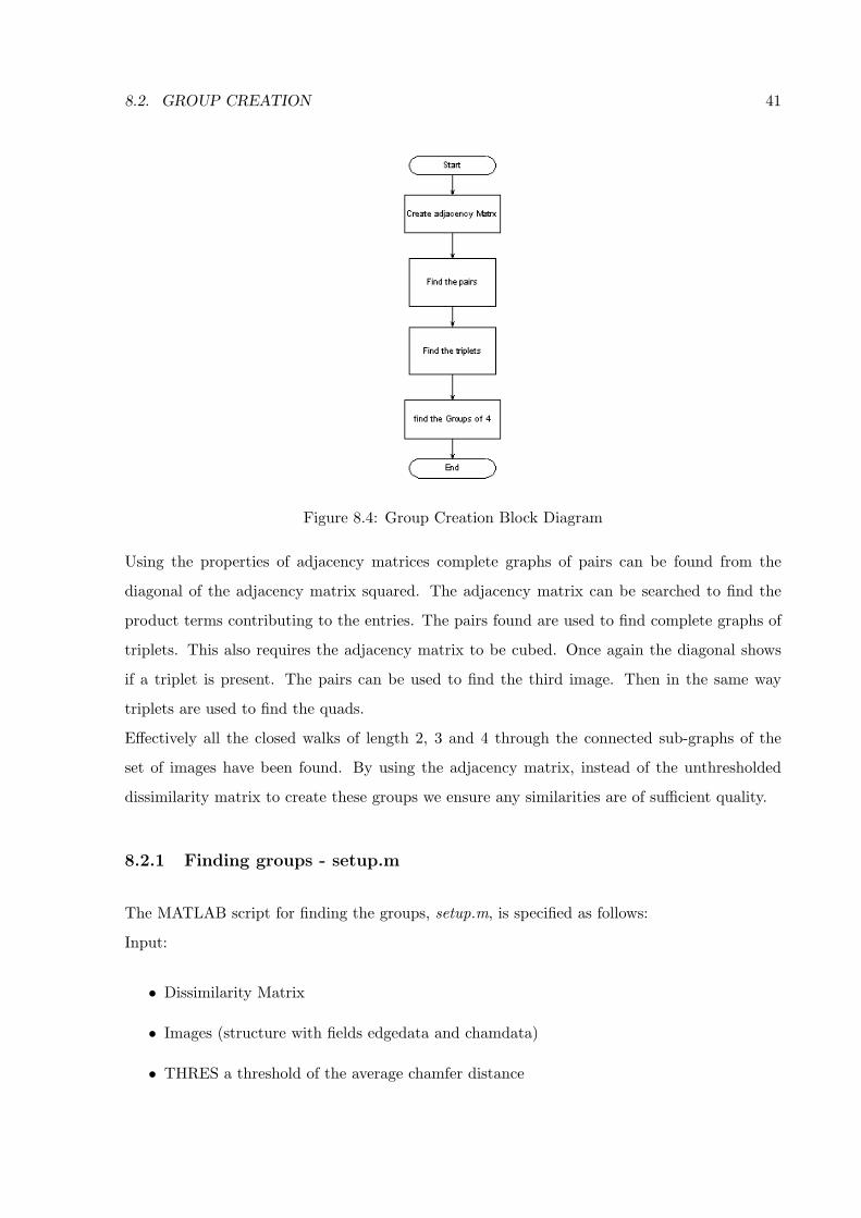
A Design Diagram is shown in figure 8.4. Groups were created by finding complete graphs within

the set of images. The graph of images was represented by an adjacency matrix. The adjacency

matrix was formed by thresholding the dissimilarity matrix. All values below the maximum

distance are set to 1 indicating the images are similar (adjacent given this threshold). This was

effectively setting a threshold on impurity to control the properties of the tree.

8.2. GROUP CREATION 41

Figure 8.4: Group Creation Block Diagram

Using the properties of adjacency matrices complete graphs of pairs can be found from the

diagonal of the adjacency matrix squared. The adjacency matrix can be searched to find the

product terms contributing to the entries. The pairs found are used to find complete graphs of

triplets. This also requires the adjacency matrix to be cubed. Once again the diagonal shows

if a triplet is present. The pairs can be used to find the third image. Then in the same way

triplets are used to find the quads.

Effectively all the closed walks of length 2, 3 and 4 through the connected sub-graphs of the

set of images have been found. By using the adjacency matrix, instead of the unthresholded

dissimilarity matrix to create these groups we ensure any similarities are of sufficient quality.

8.2.1 Finding groups - setup.m

The MATLAB script for finding the groups, setup.m, is specified as follows:

Input:

• Dissimilarity Matrix

• Images (structure with fields edgedata and chamdata)

• THRES a threshold of the average chamfer distance


Output:

• Imagestruct (structure with many fields representing groups and their intergroup and

intragroup scores)

• Adjsquare (the square of the adjacency matrix)

8.2.2 Score Calculation - createtemps.m

The scores referred to in the previous list are calculated by createtemps.m. Intragroup scores

are found by testing all the templates in a group against their combinational template distance

transform. The combinational templates are formed using the createtemps script by creating a

distance transform that is the mean of the images’ distance transforms. The worst (maximum)

score of the templates against combinational template, is the intragroup score. Thus each group

is scored by how badly it matches its template.

Intergroup scores are calculated by comparing a combinational template to all the images not

included in that template. The minimum score is taken to be the intragroup score because it

represents the best match. The goal is to reduce the intergroup similarity, hence make the best

match (minimum) as bad as possible. The scores of similarity and dissimilarity are calculated

using distance matching because this is the method of matching to be used.

Createtemps.m

The createmps script, as already mentioned, creates a combinational template. The arguments

are as follows:

Input:

• Image Number for “root” image.

• Vector of Image Numbers for all in group.

• Images - the structure containing all the image data.

Output:


• temps - the structure containing the template data (distance and edge) and scores

• Tempscore - the template intergscore

The combinational template is later thresholded to create the feature template for this possible

tree node. It is morphologically thinned to ensure that all lines are of single width. This process

reveals the common features of the template. It should ensure that combinational templates are

subsets (or close to) of the templates. Thus as explained when discussing “reverse” matching

they match as well as the actual templates.

The templates are not saved at this time simply the scores. If all templates for each group were

saved the memory necessary would start to become ridiculously large. The scores are stored,

and templates recreated later.

8.2.3 Hierarchy Creation

An arbitrary order is used to guide the initial selection of the groups. Firstly, iterate through

the order to find the highest scoring match that will fit into the hierarchy for each image not

already included (findbestnotin.m, a recursive implementation see figure A.2). Once this has

been completed all images with no possible groups, or those that haven’t already been included

are added as single images. The features being used to create and optimise the hierarchy are

the group size, intergroup and intragroup scores.

Once the hierarchy is finished the groups scores and added together to form a hierarchy score.

The hierarchy has two scores, one to represent the intragroup scores, and one for the intergroup

scores. These scores are a measure of hierarchy quality. The flowchart (Figure 8.5 shows the

procedural design of the script.

Hierarchy Creation is performed by the MATLAB script createhier.m.

Inputs:

• allpairs (vector containing all pairs already in hierarchy)

• Imagestruct (same as before)

• Order (arbitrary order of construction)


Figure 8.5: Hierarchy Creation Flowchart

• Hierarchy (the existing hierarchy, if partially built)

• NOIMAGES (number of images)

Outputs:

• hierarchy (structure with groups, scores and intergroup scores)

• Scorevect (the cumulative totals for inter and intra group scores)

8.2.4 Hierarchy Optimisation

The hierarchies are optimised with a simple method similar to the simulated annealing used

by Gavrila [4, 5]. In this case it has been greatly simplified due to limited understanding of

the mathematical concepts and time restraints. The quality of the trees is measured by the

similarity of images within a group (intragroup scores) and their dissimilarity to other groups

(intergroup scores).

A group is not allowed to be removed if it has no pairs, it has already been removed or the last

step was backwards. If the resulting hierarchy has a better score, it is kept and the annealing

process is continued. To avoid local minima the optimisation is allowed to take one step back-

wards, to a higher score, if the next score is then lower than the previous best the change is

accepted, otherwise the annealing process is finished. “Backwards” steps are not dependant on

a “temperature” factor.


This optimisation takes place in the combinegroups.m script. The optimisation is attempted

for a variety of orders. The hierarchy is created for each order using createhier.m, it is then

optimised with the anneal function. The anneal function calls the remove function each pass.

This is all represented by the flowcharts in figures 8.6, A.4 and A.3.

This is done for multiple arbitrary orders to show the effectiveness of the optimisation. For

Figure 8.6: combinegroups.m Flowchart

the ”best” hierarchy the templates are regenerated, as only template scores were saved the first

time they were created.

8.2.5 Multi-Level Hierarchy

To create a multi-level hierarchy the same functions are applied to the templates resulting from

the combination of the leaf level images. A script temps2images.m was programmed to automate

the creation of multilevel hierarchies. Alternatively if all the template images are written to files

they can be accessed with createTree to form another hierarchy.


8.2.6 Final Implementation

The final implementation has been submitted with this thesis. To use this bottom-up hierarchy

creation, you must recursively apply it to each level of the hierarchy.

1. Place the image files into the same directory.

2. Run the createtree script (edited to use that directory) to get the images and dissimilarity

matrix into the workspace.

3. Use setup1 to create the groups that are used to optimise the hierarchy.

4. Run combinegroups to combine and optimise these groups into a hierarchy. Combinegroups

will show you each group, and output as files the images of the combinational templates.

They will be named based on the number of “root” of each group.

5. Repeat this on the combinational templates for the next hierarchy level and so on.

Note: The algorithm is written recursively to make it easy (not efficient), which means it will

fail if there are too many groups. Which happens if your threshold is too low, or there are too

many images.

8.3 MATLAB Prototype Matching

A prototype matching system was created in MATLAB to help understand and refine the algo-

rithm, in an easy development environment. It was always destined to be slow and unusable,

even on static images. The basic chamfer matching algorithm was implemented using simple

forward and reverse matching. This helped to refine several techniques and test possible ap-

proaches to speeding up the matching process.

The final MATLAB matching system was different than the eventual Visual C++ real-time sys-

tem, but was an excellent learning experience. The first approach taken was a simple distance

match of one template to images, involving both forward and reverse matching. This template

could then be selected to test varying combinations of template and image. This led to the

notion of masking the reverse search to avoid non-sign details affecting the match.

8.3. MATLAB PROTOTYPE MATCHING 47

Figure 8.7: Simple Matching System

Effective matching was stifled greatly by trees. Simple colour detection and subsequent masking

of the edge detection image by the colour information was tried. The thesis was not meant

use colour information, due to previous work proving it to be unreliable, so this approach was

discontinued. Further methods tried to improve the matching included Localised thresholding,

sub-sampling of the edge detection and oriented edge detection.

Oriented edge detection did not remove the trees as possible matches but increased their “ran-

dom” appearance when compared to the well directed outline of traffic signs. They still caused

unnecessary expansion of the search, but at a fine level helped reduce false matching.

Localised thresholding (A.5.1)used simple statistical methods, first encountered during ELEC4600

to increase the threshold in areas with high edge content. This was an attempt to reduce detail

in areas of trees. Different thresholds (A.5.2) were also tried for different levels of the search.

Sub-sampling (A.5.3)of the edge detection also attempted to remove the tree data.

8.3.1 Basic System

The design of the basic fine/coarse single template distance matching system in MATLAB is as

follows (Figure 8.7):


R10simplepyroverlay.m

This file implements the design in figure 8.7. As shown it takes a recursive approach to searching

each of the starting locations, which are iterated over. After the initialisation of variables the

iterative for loop steps through each of the starting positions separated by 8 pixels vertically

and horizontally. This location is passed to a recursive loop, named expand, which searches this

sub-area.

For each search position based on the step a forward score is calculated. If this forward score is

below a threshold, the search is expanded further on this location, by recurring with a smaller

step, else the search is terminated.

Following the theory relating to coarse fine distance matching the threshold is reduced as a

function of the step. If the step is one a reverse and forward score is computed for both

locations. If there were sufficient pixels in the edge image to indicate a “sensible” reverse match

and the product of the forward and reverse threshold a match is considered to be found. If these

conditions are not met the search is terminated without a match being found.

8.3.2 Masking Reverse Search

This simple search was improved by masking the reverse search. The reverse search is only

appropriate for areas included within the boundaries of a sign. For example if a sign is surrounded

by Trees the edge detection may look as in figure 8.8. Setting the region of interest to the square

Figure 8.8: Noise Behind Sign

shape of the matrix will cause the tree edge detection to inflate the reverse score. By masking

the edge detection with figure 8.9. The region of interest is changed to include solely inside

the boundaries of the sign. Ensuring the only features considered are those of the sign, not the

background. This matched individual templates well. The search still expanded unnecessarily

on areas of noise, like trees, and gave some false matches.


Figure 8.9: Reverse Matching Mask

8.3.3 Pyramid Search

This pyramid search used the hierarchy object created by the MATLAB script described in the

previous section. This implementation is much more complicated than the simple search as the

hierarchy must be searched concurrently with the coarse/fine matching.

The following design (Figure 8.10) was used to search each group for a match:


Figure 8.10: Pyramid Search


It was implemented in pyroverlay.m and was a simple iteration through each member of the

group. Another function simply called each group. Work on the pyramid search was very brief

due to the poor results of the simple one template fine coarse search. Refinements were need to

the matching design to improve accuracy and precision.

Oriented Edge Detection

Oriented edge detection has been used by other researchers in matching problems, including

hierarchical searches, so the expectations were high. The planned implementation was to modify

the existing canny edge detection algorithm in MATLAB to produce a binned orientation map.

The canny edge detector already estimates the direction of edges for use in the non-maximal

suppression. By binning the values during this calculation the output from the canny edge

detector could be scaled with different magnitudes representing orientations. Directions are

binned based on the following diagram:

% The X marks the pixel in question, and each

% 3 2 of the quadrants for the gradient vector

% O----0----0 fall into two cases, divided by the 45

% 4 | | 1 degree line. In one case the gradient

% | | vector is more horizontal, and in the other

% O X O it is more vertical. There are eight

% | | divisions, but for the non-maximum supression

% (1)| |(4) we are only worried about 4 of them since we

% O----O----O use symmetric points about the center pixel.

% (2) (3)

(From MATLAB image processing toolbox edge function)

The edge function iterates over the directions, finding the maximums for each. The edge pixels

for each direction are placed in another matrix (three dimensional) directionmatrix. Shown in

A.4.1 is the section of code changed. I can then output a matrix with edges directionally coded

into the magnitude (Figure 8.11).


Figure 8.11: Oriented Edge Detection

8.3.4 Directional Matching

To match the oriented edge detection to the template requires a “oriented edge map” of the

template. By extending the distance transform to produce a matrix labelling every position

with the direction of the closest template feature pixel allows a comparison of the distance

between image and template pixels and a “distance” between their direction.

Directionchamfer.m was the script to perform this function, after calculating the result of the

minimum distance (split into positions which have 4 added to them and 3), a position then

inherited the direction of the pixel that its minimum distance was calculated from. The code in

A.4.2 was iterated over the template image. Equating the following: diri,j = dir(min(vk−1i−1,j−1 +

4, vk−1i−1,j + 3, vk−1

i−1,j+1 + 4, vk−1i,j−1 + 3, vk−1

i,j , vk−1i,j+1 + 3, vk−1

i+1,j+1 + 4, vk−1i+1,j + 3, vk−1

i+1,j+1 + 4)) Results

of this for the image shown in figure 8.11 are shown in figure 8.12.

This was too expensive to perform on the entire image, so it was only implemented for forward

matching against the distance transform of the template. A more efficient distance transform

method may have been possible, but as this was a prototype implementation designed to test

the algorithm it was not attempted.

The oriented distance matching was implemented for single image coarse fine matching. The

script written was simplepyrdirectedoverly.m.

Positions were expanded based on the forward matching as before, but confirmation of matches

used the forward, reverse and orientation matching scores. This rejected almost all of the false

matches, allowing the results presented in my thesis seminar.


Figure 8.12: Orientation Map

The orientation matching score was calculated using the following formula: For every pixel in

the directed edge image subtract the value of the corresponding pixel in the direction map then

Mod that with three. This results in the following scores:


Edge Score Orientation Map Matching Score

1 1 0

1 2 1

1 3 2

1 4 1

2 1 1

2 2 0

2 3 1

2 4 2

etc...

Table 8.1: Directional Scoring


8.3.5 Rejected Refinements

Some rejected refinements to the system are present in Appendix A.5.

8.3.6 Final Implementation

A final implementation for the MATLAB prototype Matching was not delivered. The work was

always intended to aid in understanding of the Algorithm. The work was left “unfinished” and

implementation of the real-time system was started.


8.4 Real-Time

The design for the real-time implementation would reflect the properties of the matching al-

gorithm discovered in the prototype implementation. The basic forward and reverse matching

design would be implemented first. If additional accuracy proved necessary this could be ex-

panded to include orientation matching. The procedural diagram of the matching algorithm,

based on the prototyping, to be implemented was as figure 8.10.

8.4.1 Matching Process

Figure 8.10 shows the initial procedural design for the matching algorithm simplified to the

main processes. Each template root is forward scored against positions. Based on this score the

position is expanded to include sub-positions. If the matching reaches the minimum step the

hierarchy search is enacted. This will search the children of each root, expanding on the best

match above the threshold. If the leaf level of the tree is reached, a reverse match is calculated

confirming the presence.

Reverse matching cannot be used until the leaf level of the matching process because combina-

tional templates may not include every feature of the leaf template they represent. They only

contain the common features of their leaves.

8.4.2 Object Oriented Design

The system was designed in an object oriented environment. Hence Object Oriented design

concepts were used. The following initial design (Figure 8.13) was established prior to imple-

mentation. These intended designs are the ideal situation where the search is handled within

the template classes. An abstract builder pattern is used to create the trees. The class diagram

(Figure 8.13) shows the main classes and their main features important to the matching algo-

rithm.

The EZrgb24 class contains the image data. This includes the edge image, distance image and

the output image. The transform method is part of the original example code. It is executed on

each frame, and is where the edge detection and distance transform will be effected. EZrgb24

8.4. REAL-TIME 57

Figure 8.13: Intended Class Diagram

will also write the output to the stream.

The mytree class is an abstract builder. It has subclasses that are concrete builders, actual

implementations. The mytree class allows the polymorphism to be used. Any of the concrete

builders can be implemented at run-time, and can use the same interface. The builders are

invoked to create the tree of templates. The constructor creates the mytemplatev objects in the

appropriate hierarchy. It allows other classes access to the hierarchy through the array of root

templates.

The mytemplatev class contains and operate on the template data. It has methods to score and

search through the image hierarchy. Each template contains its distance and edge data and a

pointer to its array of children. Their are methods for EZrgb24 to access the data.

Sequence Diagram

The sequence diagram figure (A.7) shows the flow of control between process and objects. This

design is simplified due to my limited knowledge of UML.

The EZrgb24 object is responsible for creating the IplImage objects to represent the images. It


also creates a mytree object and instantiates it with whichever tree is necessary for the matching

task. This builder class creates the template hierarchy.

For each frame the transform method is executed. This (not shown in diagram) allocates the im-

ages with the calculated edge and distance transforms. For each position to be search, transform

runs the hierarchy search. The template class then takes care of forward and reverse scoring

appropriately through the hierarchy (not shown in detail). Scores and details of the found image

are returned to the Ezrgb24 object to be written to the output.

This design allows the template details to be completely hidden from the EZrgb24 object by

encapsulation within the mytemplatev object, until a match is found.

Obviously at the completion of each frame the transform filter will be run again. (Not Shown

in diagram.)

8.4.3 Actual Design

By reverse engineering the code actually written I am able to present the actual design imple-

mented. The class diagram A.8 of the actual implementation shows that the EZrgb24 class has

responsibility for most of the scoring and searching methods. The mytemplatev class has almost

become an abstract data type. This change in design was necessary during the programming of

the thesis. The IplImage objects require careful maintenance to prevent memory leaks. It was

much simpler to keep all references and use of this data within the transform method and not

“pass” it to the template objects, even as a reference to a static attribute. Reverse scoring is

still run in this method, but memory deallocation cannot be properly controlled without causing

errors. Due to the limited nature of reverse scoring this memory leak is allowed to continue to

demonstrate the intended design.

As can be seen, this design does not merge the coarse/fine search into the hierarchy search.

If this were included as indicated in the theory, the threshold must be constantly modified by

step and template to combination template parameters. Separating the searches simplified the

programming task. If the results were poor, it could have been added later.

The classes have also become too big. Ideally in object oriented design the analysis phase should

ensure that the classes are minimal and do not implement too much functionality.

The basics of tree building are kept the same in this design. The diagram also shows more of the

8.4. REAL-TIME 59

implementation details ie. private variables, but without showing all the private methods needed.

Sequence Diagram

The sequence diagram A.9 reflects these changes made to the class diagram. It can be easily

seen it is overcomplicated, and control resides mainly within the transform filter.

Firstly a coarse/fine search is executed with the root templates at each position. This forward

searches the root templates until the step is one. This may be expanded to the hierarchical

search based on the scores. At the leaf nodes a reverse search is executed. The output is written

similar to before. The function is greatly simplified because the transform method knows which

template matches (because it generated the scores).

8.4.4 Further Information

Appendix A.7 explains in more detail how some difficult parts of the implementation were

achieved.

8.4.5 Enhancements/Refinements

The following enhancements and refinements were implemented on the real-time system:

• Spiralling out from the centre of the ROI

• Temporal Filtering to remove trees

• Oriented Edges

• Expanding all possibilities or best

• Reverse Scoring

• Truncating the Distance Transform

These are explained in detail in Appendix A.8


8.4.6 Final Matching Algorithm Used.

The final matching algorithm implemented used the maximum, truncated and scaled distance

matching approaches. Only the best match at each level of the hierarchy was expanded. Oriented

edge detection was not fully implemented in the real-time environment as match accuracy was

reasonable. Temporal filtering was also unnecessary. The spiral search pattern was rejected as

the matching may need to find multiple objects, due to false matches.

8.4.7 Further Examples

Some further examples were programmed to prove the possibilities of the matching algorithm.

• Letter Matching

• Size Variance Matching

• Deformable Contour Matching

Letter Matching

Many of the improvements mentioned were discovered by using a simplified matching case,

that of letters. Traffic sign footage contains many uncontrollable variables, such as lighting,

occlusions, trees, damage, car movements. By creating a hierarchy of letters, the matching can

be demonstrated and tested in real-time in the lab. The hierarchy works on text of a known

font, creating the templates using bitmaps of the letters, and providing the letter images, by

printed out copies, in a very large font. The hierarchy is interchangeable with the traffic sign

hierarchy thanks to polymorphism. This system allowed the results of many of the refinements

to be tested. And some of the refinements/bugs were discovered by preparing this easier case.

Size Variance Matching

Hierarchical chamfer matching can be employed to create a size variant matching system. By

creating a hierarchy of differently sized objects they can all be searched for simultaneously.

8.4. REAL-TIME 61

The hierarchy is generally formed by grouping similarly sized objects, for example (Figure A.1.

In this application, where masking of the reverse search is used, this would also require a

different mask for each template, instead of different masks for subtrees (circle, diamond, etc...).

Due to this added complication, the example application realised used simple circles on a plain

background.

Figure 8.14: My Size Variant Hierarchy

Rotational Matching

Another possible scenario, as already mentioned, are rotations of objects. Most rotations bare

a similarity to the previous and next rotation. By exploiting this, a hierarchy can be created of

similar rotational shapes.

Chapter 9

Results

9.1 Hierarchy Creation

The hierarchy creation code could successfully optimise small hierarchies. When given a rela-

tively low threshold, the results were not affected by the order of images therefore were optimised.

If the threshold was high, the results were the same for groups of similar orders.

The creation system was designed around recursive programming. This allowed problems to

be simplified, however, it did not create an efficient system. Due to memory constraints large

hierarchies and those with many combinations (i.e. low threshold) should be avoided.

9.1.1 Hierarchies

Selected results generated by the hierarchy creation are included.

Diamond Signs

The hierarchy included in A.9.1 is of a sub-set of diamond sign templates to demonstrate the

effectiveness of the automated hierarchy creation.

The following commands were used:

63

64 CHAPTER 9. RESULTS

[diss, images]= createTree;

[imagestruct, adjsquare]= setup1(diss, images, 0.5);

[hierarchy, temps, options] = combinegroups(images,

imagestruct, 0.5, adjsquare);

The scores achieved by each order before optimisation are presented in figure A.14. After

optimisation it can be seen (figure A.15) that groups with similar starting orders have given the

same score, hence some “optimisation” has been achieved.

Circular Signs

A Hierarchy of Circular signs was generated in a similar manner. The following figure represents

the hierarchy created. The scores achieved are represented in figure A.36. They demonstrate

Figure 9.1: Circular Sign Hierarchy

an “optimal” solution has probably been achieved, because no matter what order the hierarchy

was created in the result was the same.

Others

Hierarchies for letters, multi-resolution and deformable contours are not included due to size

restrictions on this document.

9.2. MATLAB MATCHING 65

9.2 Matlab Matching

The basic system of single template matching has limited possibilities. It produced similar scores

for an exact match as it did for noise-like patterns created by the edge detection of trees. The

addition of reverse matching had limited success. Using a Hierarchical search in this situation

did not improve the matching.

The first major improvement to matching accuracy was made by the masking of reverse scoring

(8.3.2). This refined the sign matching but still allowed unnecessary search expansion.

Localised thresholding as a means to limit unnecessary expansion of the search, proved com-

putationally expensive (Figure A.6). So did matching in different feature extractions. Using

additional oriented edge information, increased the accuracy and precision of the match. There

was only a slight increase in computational expense, due to the exploitation of the canny edge

detection. This still did not limit the search’s tendency to expand in places that contained dense

edge information, such as trees.

9.2.1 Matlab Matching Results

The diagrams in A.10 detail the results achieved in the MATLAB matching prototype. Which

was able to match signs in static images.

9.3 Real-Time Matching

The results presented on traffic sign detection show that a real-time detection system based

on Hierarchical Chamfer Matching built for a general purpose platform is a realistic goal. The

development of the algorithm provided some insights into valuable enhancements.

The ideas rejected include the spiral search pattern, simple temporal filtering, and expanding

“all” matches below the threshold. The use of truncated distances was retained. Oriented edge

were not implemented but results indicate that this or another stage may still be necessary for

match verification.

The matching algorithm is intolerant to poor edge detection. In much of the footage recorded


the sign is blurred as it nears the correct size for matching, probably due to automatic focussing

of the camera. This blurring reduces the quality of the edge detection, which means features

are missing from the image and a good forward match is not possible. In other examples, such

as letter matching, the results are much better due to the controlled environment.

9.3.1 Performance

On a 1.6Ghz Pentium 4 with 256 Meg of RAM the frame rates varied bfrom over 20 frames/second

in scenes were there was little noise to cause unnecessary expansion, to under 10 frames a second

for more difficult scenes. These results were on video that was 360× 288 pixels.

9.3.2 Results

Virtually all traffic signs that were edge detected without distortion were found. False matches

were infrequent and limited to noisy sections. The images here (figures 9.2 and 9.3) show the

system output. The biggest problem affecting matching was the poor edge detection resulting

from blurred footage.

Figure 9.2: 50 Sign

9.3. REAL-TIME MATCHING 67

Figure 9.3: 60 Sign

9.3.3 Letter Matching

A hierarchy was created using the alphabet in a known font. This further demonstrated hierar-

chical matching. Results proved that print-outs of letters could be matched when held in front

of a USB camera, with virtually no false matches in an “office” environment. This was once

again in real-time.

9.3.4 Size Variant Matching

The demonstration of matching over 20 different sized circles, at a high frame rate, has shown

that this algorithm could be suitable for matching an object of unknown size. By creating a size

hierarchy, then using an object type hierarchy a very large number of shapes and sizes could be

recognised.

9.3.5 Rotational Matching

A simple cross pattern was sampled at varying rotations and placed into a hierarchy. This

demonstrated the algorithm’s ability to match rotations of objects. By combining rotations

with scaling and skews in a large hierarchy, a very robust detection system would be possible.


9.4 My Performance

9.4.1 Skills Learnt

During the course of this thesis I have learnt many new skills. These included graph theory,

image processing and object oriented programming.

I learnt several graph theory concepts and the basics of constructing a tree. I greatly expanded

my mathematical knowledge of image processing, particularly edge detection, distance trans-

forms and matching metrics.

My Visual C++ programming skills were improved due to the complicated nature of the match-

ing algorithm. I also benefitted from investigating the OpenCV library in great detail.

9.4.2 Strengths/Weaknesses

My main weakness was object orientated design and the ability to realise that design. I was

unable to build a well structured program. With the knowledge gained during the thesis I could

perform much better if the application were to be programmed again.

My strength is knowledge, experience and understanding of Image Processing Algorithms. This

allows me to quickly evaluate possible approaches based on results of prototyping.

Chapter 10

Future Development

Several aspects of this thesis could be improved if future work was conducted.

• More consistent video footage

• Temporal Information included

• Better Object Oriented Design

• Improved Hierarchy Generation

• Optimisation

• Final verification stage

10.1 Video Footage

The fixation of a camera to the vehicle and the use of a more suitable camera would increase the

consistency of footage. A clearer image would allow better edge detection and therefore better

matching.

69

70 CHAPTER 10. FUTURE DEVELOPMENT

10.2 Temporal Information

The use of temporal information in the application would increase the quality and speed of

matching. Tracking of potential signs from frame to frame and use of the expected paths of

traffic signs could help to speed up matching by pin-pointing likely locations.

10.3 Better OO Design

If the design were more complete and could be effectively realised, the quality of code may be

increased. This would not necessarily make it faster, but would increase the readability. Design

methods for speed of applications in the environment should be studied further.

10.4 Improved Hierarchy Generation

If the MATLABtm system was able to handle larger image databases, and automatically generate

the concrete builder in c++/pseudocode the application would be easier for developers to use.

Changes in hierarchy would be simpler. Larger hierarchies could also be created.

10.5 Optimisation

After the design was improved and the code simplified effort could be spent improving the

efficiency. A faster application would allow larger hierarchies and hence more robust matching.

Further improvements would be possible if unnecessary expansion caused by noise, such as trees,

could be stopped.

10.6 Final Verification Stage

A final verification stage such as using orientation information (similar to the MATLAB proto-

type), colour or neural network stage [4, 5].

Chapter 11

Conclusions

This thesis proved that the hierarchical distance matching algorithm is effective for many image

processing scenarios, in particular traffic sign recognition. It is worthy of further investigation

and development. The traffic sign matching application developed has proven that “smart”

vehicle systems are not far away from mass production.

The goals of the thesis were achieved. A hierarchy creation system was implemented in MAT-

LAB. The matching was then prototyped, again in MATLAB. This allowed various parameters

and properties of the metric to be explored. A real-time matching application was built utilis-

ing the IPL Image Processing and OpenCV libraries. It was also expanded to other matching

scenarios.

The hierarchy creation system that has been developed will create and optimise a structure. It

uses graph theory concepts derived from [2]. The output of this can be used in both the static

and real-time matching systems.

A simple static matching system was developed to prototype the algorithm outlined in [4] and

[5]. It is incomplete but matches single templates on images with high accuracy yet poor time

performance.

The real-time system is dependant on quality video footage, but can produce excellent results.

It is capable of recognition up to 20 frames per second. Very few false matches are detected.

This document contains the assumptions and a brief specification of the recognition system. Rel-

evant literature has been reviewed to provide theoretical basis for this thesis. Implementation

and design details of both hardware and software are included. As are results, recommendations

71

72 CHAPTER 11. CONCLUSIONS

for future work and conclusions.

Chapter 12

Publication

Extract from article to be published in UQ News on the 20th of October.

12.1 Australia’s Innovators Of The Future

Craig Northway’s Real-Time Traffic Sign Recognition project is based on the work of

Daimler Chrysler Research, which hopes to develop Smart Cars that avoid pedestri-

ans and remind you of the speed limits. If the project is developed further, vehicles

could soon have the ability to warn drivers of pending situations or automatically

take evasion action.

Craig’s supervisor Associate Professor Brian Lovell said he hopes the device will be-

come marketable. It involves the use of a camera mounted in the car. A computer

processes the information into (sic) real time, he said. He also told how the project

would be demonstrated at a transport mission in Ireland later in the year.

73

74 CHAPTER 12. PUBLICATION

Bibliography

[1] C. Olson and D. Huttenlocher, “Automatic target recognition by matching oriented edge

pixels,” IEEE Transactions on Image Processing, vol. 6, no. 1, pp. 103–113, 1997.

[2] S. Aksoy and R. M. Haralick, “Graph-Theoretic Clustering for Image Grouping and Re-

trieval,” IEEE Conf. on Computer Vision and Pattern Recognition, 1999.

[3] G. Borgefors., “Hierarchical chamfer matching: A parametric edge matching algorithm,”

IEEE Transactions on Pattern Analysis and Machine Intelligence, vol. 10, pp. 849–865,

1988.

[4] D. M. Gavrila, “Multi-feature hierarchical template matching using distance transforms,”

In Proc. of the International Conference on Pattern Recognition, pp. 439–444, 1998.

[5] D. Gavrila and V. Philomin, “Real-time object detection for ”smart” vehicles,” In Inter-

national Conference on Computer Vision,, pp. 87–93, 1999.

[6] G. P. et. al, “Robust method for road sign detection and recognition,” Image and Vision

Computing, vol. 14, pp. 109–223, 1996.

[7] J. Logemann, “Realtime traffic sign recognition.” Web Site, last viewed on 30/03/02.

[8] J. M. et al, “An active vision system for real-time traffic sign recognition,” 2000.

[9] G. Saligan and D. H. Ballard, “Visual routines for autonomouis driving,” 1998.

[10] M. Betke and N. C. Markis, “Fast Object Recognition in Noisy Images using Simulated

Annealing,” 1993.

75

76 BIBLIOGRAPHY

[11] D. Rogahn, “Road sign detection and recognition.” Web Site, last viewed on 23/03/02,

2000.

[12] P. Dhanaraks and N. Covavisaruch, “PLANAR IMAGE MOSAICING BY HIERARCHI-

CAL CHAMFER MATCHING ALGORITHM,” 1998.

[13] G. K. D. Huttenlocher and W. Rucklidge, “Comparing images using the hausdorff distance,”

IEEE Transactions on Pattern Analysis and Machine Intelligence, vol. 15, pp. 850–863,

1993.

[14] W. Rucklidge, “Locating objects using the hausdorff distance,” In Proc. of the International

Conference on Computer Vision, pp. 457–464, 1995.

[15] C. Olson, “A probabilistic formulation for hausdorff matching,” In Proc. of the IEEE Con-

ference on Computer Vision and Pattern Recognition, 1998.

[16] S. Lu and A. Szeto, “Hierarchical Artificial Neural Networks for Edge Enhancement,” Pat-

tern Recognition, vol. 26, no. 8, pp. 427–435, 1993.

[17] P. S. E. O. M. Oren, C. Papageorgiou and T. Poggio, “Pedestrian detection using wavelet

templates,” In Proc. of the IEEE Conference on ComputerVision and Pattern Recognition,

pp. 193–199, 1997.

[18] R.-L. H. M. A.-M. A. K. Jain, “Face Detection in Color Images,” 2001.

[19] Estevez and Kehtarnavaz, “A real-time histographic approach to road sign recognition,”

Proceedings of the IEEE Southwest Symposium on Image Analysis and Interpretation, 1996.

[20] Q. Iqbal and J. K. Aggarwal, “Perceptual Grouping for Image Retrieval and Classification,”

Third IEEE Computer Society Workshop on Perceptual Organization in Computer Vision

(POCV01), pp. 19–1–19–4, 2001.

[21] R. Turcajova and J. Katsky, “A hierarchical multiresolution technique for image registra-

tion,” 1995.

[22] E. C. H. Jr. and F. King Sun, “A non-parametric positioning procedure for pattern classi-

fication,” IEEE Transactions on Computers, vol. 7, pp. 614–624, 1969.

BIBLIOGRAPHY 77

[23] R. Z. Jing Huang, S Ravi Kumar, “An Automatic Hierarchical Image Classification

Scheme,” 1999.

[24] S. K. M. Abdel-Mottaleb, “Hierarchical clustering algorithm for fast image retrieval,” Part

of the IS and T SPIE Conference on Storage and Retrieval for Image and Video Databases

VII, pp. 427–435, 1999.

[25] G. Borgefors, “Distance transforms in digital images,” Computer Vision, Graphics and

Image Processing, vol. 34, pp. 344–371, 1986.

[26] A. E. Johnson and M. Hebert, “Recognzing objects by matchin oriented points,” IEEE

Computer Vision and Pattern Recognition, CVPR ’97, 1997.

[27] R. J. Wilson and J. J. Watkins, Graphs An Introductory Approach. John Wiley and Sons,

New York, 1990.

[28] W. K. Grassmann and J. paul Tremblay, Logic and Discrete Mathematics. Prentice Hall,

New Jersey, 1990.

[29] K. Venkata and S. Murthy, On Growing Better Decision Trees from Data. PhD thesis,

Johns Hopkins University, 1997.

78 BIBLIOGRAPHY

Appendix A

A.1 Assumptions

A.1.1 Speed

The camera must be able to resolve a sharp image from a fast moving vehicle. For demonstration

purposes footage can be taken from a slow moving vehicle. This can prove the potential of the

algorithm. In a smart vehicle system the camera must be able to resolve images at speeds of up

to 110km/h.

A.1.2 Lighting

The lighting during the filming should be reasonable, such that once again the camera can

resolve the image. Once again in a smart vehicle system a high quality camera capable of

low light filming would be used. Due to the reflective nature of traffic signs, detection can be

performed at night using this method [4, 5].

A.1.3 Position

It is reasonable to assume that the traffic signs consistently appear in a similar region of the

video footage. If the camera was mounted on the dash of a vehicle, the signs would tend to pass

through the same area of the footage (Upper Left in Australia).

79

80 APPENDIX A.

A.1.4 Angle

The relative angle between the car and the sign is close to perpendicular. If the car were in

an extreme right lane, the image of the sign would be skewed severely. The HCM algorithm is

unable to rectify this situation, without incorporating these skewed images into the hierarchy.

A.1.5 Damage

Signs must be assumed to be undamaged. Signs that have suffered damage may be bent, twisted

or missing sections. Small amounts of damage should not affect the matching. It is fair to assume

that most signs are relatively undamaged, as they are regularly maintained by local governments.

A.1.6 Size

Invariance Due to the Size invariant nature of the algorithm it must be assumed that the signs

pass through this size(s) as the car approaches them without being obscured. In the Daimler

Chrysler system [4, 5] sign templates are two sizes, reducing the chance of them being ”missed”.

Figure A.1: Multi-Resolution Hierarchy [4]

A.1. ASSUMPTIONS 81

A.1.7 Computer Vision Functions

The following assumption relates to the Computer Vision functions present in the IPL and Open

CV libraries. The Edge Detection should give a reliable single line outline of the signs. If the

functions are correct they should be able to produce an edge detection of the signs in most

circumstances based on set thresholds providing the video meets the previous assumptions.

A.1.8 Objects

One major assumption must be made about the shapes to be detected. For HCM to be effective

the shape of the objects should be similar. Traffic signs fulfil this assumption, as there are

a limited number of signs that are easily grouped into basic outline shapes. For example a

hierarchy of fruits and vegetables might be unsuccessful. The comparative shapes of bananas,

oranges and potatoes are dissimilar. Even within one type of fruit, such as bananas there is

sufficient variation with similarities to create a hierarchy of bananas alone. Thus Traffic signs,

text of known font, car outlines, are predictable shaped similar objects suitable for HCM.

82 APPENDIX A.

A.2 Programming

A.2.1 MATLAB

MATLAB will not be new to most electrical engineers. It is a numerical mathematics package,

able to be programmed using m-files in language similar to C or Java. It can be compiled at

run-time or pre-compiled into dlls. It is untyped allowing fast prototyping of algorithms, but

not with sufficient structure or speed for extensive programming.

A.2.2 Direct Show

Direct show is Microsoft’s architecture for streaming media. In this system streams originate, are

operated on and end in filters. Filters are joined by COM objects. A graph of filters is created.

This could be hard coded or, by using an application from the SDK, designed graphically.

Filter graphs start with a source, e.g. File Source, USB Camera, TV tuner, are operated on

by filters such as splitters, decompressors etc.. and displayed by renderers or written to files by

writers. For more information see: http://msdn.microsoft.com/default.asp

A.2.3 IPL Image Processing Library

The IPL Image Processing library was created by Intel to use their extended MMX instruc-

tion set. This uses SIMD instruction sets to perform efficient operations on media such as

audio and video. SIMD stands for single instruction multiple data and is advantageous in

situations where recurring operations are made to large amounts of data such as in signal

processing. This has since been discontinued as a free download. For more information see:

http://www.intel.com/software/products/perflib/ijl/index.htm

A.2.4 Open CV

The open source computer vision library is available free of charge for research purposes from

http://www.intel.com/software/products/opensource/libraries/cvfl.htm. Image data structures

A.2. PROGRAMMING 83

from the IPL imaging library are used extensively. It is a set of more complex image processing

functions compared to the IPL library.

84 APPENDIX A.

A.3 Extra Hierarchy Implementation Flowcharts

Figure A.2: findbestnotin.m Flowchart

A.3. EXTRA HIERARCHY IMPLEMENTATION FLOWCHARTS 85

Figure A.3: anneal.m Flowchart

86 APPENDIX A.

Figure A.4: remove.m Flowchart

A.4. PROTOTYPE ORIENTATION CODE 87

A.4 Prototype Orientation Code

A.4.1 Orientated Edge Transform

for dir = 1:4

e2 = repmat(logical(uint8(0)), m, n);

idxLocalMax = cannyFindLocalMaxima(dir,ax,ay,mag);

idxWeak = idxLocalMax(mag(idxLocalMax) > lowThresh);

e(idxWeak) = 1;

e2(idxWeak) = 1;

idxStrong = [idxStrong; idxWeak(mag(idxWeak) > highThresh)];

%this should create a direction map...

rstrong = rem(idxStrong-1, m)+1;

cstrong = floor((idxStrong-1)/m)+1;

e2 = bwselect(e2, cstrong, rstrong, 8);

e2 = bwmorph(e2, ’thin’, 1); % Thin double (or triple) pixel wide contours

directionmatrix(:,:,dir) = dir.*(im2double(e2));

end

A.4.2 Orientation Map

fours = ([edge(i-1, j-1) edge(i-1, j+1) edge(i+1, j-1) edge(i+1,

j+1)]); threes = ([edge(i-1, j) edge(i+1, j) edge(i, j-1) edge(i,

j+1)]); if (min([threes fours])<40)

[fourmin, fourpos] = min(fours);

[threemin, threepos] = min(threes);

if (fourmin > threemin)

if (threemin < edge(i,j))

newedge(i,j) = threemin + 3;

if (threepos > 2)

direction(i,j) = direction(i, (j-1+(threepos - 3)*2));

else

88 APPENDIX A.

direction(i,j) = direction((i-1+(threepos-1)*2), j);

end

end

else

if(fourmin < edge(i,j))

newedge(i,j) = fourmin + 4;

if (fourpos > 2)

direction(i,j) = direction(i+1, (j-1+(fourpos - 3)*2));

else

direction(i,j) = direction(i-1, (j-1+(fourpos - 1)*2));

end

end

end

end

A.5. REJECTED PROTOTYPE IMPLEMENTATIONS 89

A.5 Rejected Prototype Implementations

A.5.1 Localised Tresholding

Localised Tresholding was investigated as a technique to remove the noise caused by trees. The

localised thresholds were to be applied using the canny edge detector. The standard MATLAB

edge detection command when used without parameters adjusts the threshold such that 70% of

the pixels are registered as on. This is shown in this command:

highThresh = min(find(cumsum(counts)

> PercentOfPixelsNotEdges*m*n)) / 64;

where PercentOfPixelsNotEdges = 0.7.

This would allow edges to be found, even if the maximum gradients were very low. Assigning one

global threshold for the whole image in a situation such as traffic sign recognition, where there

are many different areas, with many different textures and lighting conditions is not appropriate.

In examples such as this classic figure A.5.

Where the image contains few “textures” A global threshold is excellent. A localised threshold

Figure A.5: Simple Image

for each section of the image would provide better edge detection. In areas of low gradients, the

threshold could be lowered to detect fine details, whereas in higher gradient areas the threshold

could be increased to show fewer edges.

An informal statistical study of sections of tree image was conducted to see if any recognisable

90 APPENDIX A.

Figure A.6: Localised Thesholding

characteristics of tree gradient detection could be found to raise the threshold in these areas.

This would result in only major edges of the trees being found. As expected, areas of tree

contained high average gradients with high standard deviations. There were many edges and

hence variations in gradients. Unfortunately the same was true of the “inside” details of signs.

By localising the threshold based on the mean and/or standard deviation of the gradient image

in that region it was possible to keep only the major features of the trees and signs. This was

achieved by setting an average threshold, similar to the MATLAB default, but raising it if the

mean/standard deviation passed a certain threshold. As the results of this thresholding method

show (figure A.6, the major features were kept, and this feature detection could have been used

in the first stage of a matching hierarchy to determine sign type, and rough position. The

following code demonstrates the thresholding:

sigma = std2(image); [m,n] = size(image); EX = median(image(:));

thres = EX + 1*sigma; thres = thres/max(image(:));

lowthres = EX/max(image(:));%thres - 1*sigma/max(col);

if (lowthres >= thres)

%std is really low

A.5. REJECTED PROTOTYPE IMPLEMENTATIONS 91

thres = 0.99;

lowthres = 0.98;

end if thres < minthres

thres = minthres;

lowthres = minthres - 0.05;

end

Even though this provided a reasonable starting point for the search these calculations, standard

deviation and mean, were computationally expensive, so a quicker method was sought.

A.5.2 Different Feature Extractions

A simpler method of implementing the same concept could have been using different levels of

feature extraction for each level of the hierarchy. It becomes expensive to produce multiple

feature extractions of the same image in MATLAB. Even when a custom canny edge detection

was implemented to allow the use of the same gradient image every time. The custom canny

edge detection did not perform well and was rejected in favour of other possible solutions.

A.5.3 Sub-Sampling

By sub-sampling the edge detection it was hoped the general shape of the sign would remain,

but the trees would “disappear” or become more random compared to the distinct outline shape

of the traffic signs. It proved very difficult to sub-sample and retain the shape of the sign, as

they were being detected at the smallest possible size at which the features could be resolved

with the edge detection. This was to ensure they are detected as early as possible.

92 APPENDIX A.

A.6 UML of Real-Time System

Figure A.7: Intended Sequence Diagram

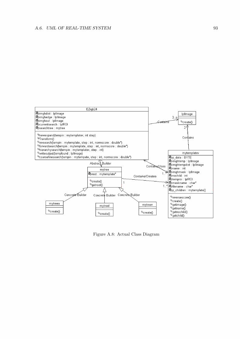
A.6. UML OF REAL-TIME SYSTEM 93

Figure A.8: Actual Class Diagram

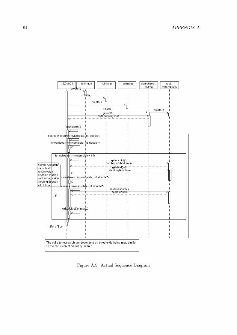
94 APPENDIX A.

Figure A.9: Actual Sequence Diagram

A.7. CODE DETAILS OF REAL-TIME SYSTEM 95

A.7 Code Details of Real-Time System

Some of the functions from the IPL Image Processing Library were used and should be docu-

mented. Other complex sections of code where commenting may not be sufficient are shown.

A.7.1 Distance Transform

When using a distance transform, and as presented later, it is necessary to truncate the values.

This can be done when scaling the image type from floating point to integer.

In this first example the data is scaled such that only distances rom 0-5 are included in the

output. This will evenly place these values from zero to the maximum of the data type being

scaled to. Thus 5 will be ≈ 255, 4 ≈ 200 ..., 1 ≈ 50, 0 = 0.

cvDistTransform(imghinv,imghgray32F, CV_DIST_L2, CV_DIST_MASK_5,

NULL); iplScaleFP(imghgray32F, imghtempdist, 0, 255);

This second example from the template creation scales the distances such that all values that

could be represented by an 8-bit unsigned integer are output. It then truncated this at 5, and

scales it such that each distance is ten times its value. Thus 5 = 50, 4 = 40, etc...

cvDistTransform(imghinv,imghgray32F, CV_DIST_L2, CV_DIST_MASK_5,

NULL); iplScaleFP(imghgray32F, imghtempdist, 0, 255);

iplThreshold(imghtempdist, imghmult, 5);

iplMultiplyS(imghtempdist, imghtempdist, 10); iplAdd(imghtempdist,

imghmult, imghtempdist);

A.7.2 Deallocation

Deallocation when using IplImage objects seems difficult. Especially when referencing them

across classes. The structure and header must always be deallocate. In some instances of

referencing, destroying the header has caused problems. So in these situations only the image

data is deallocated.

96 APPENDIX A.

iplDeallocateImage(imgh);

iplDeallocate(imgh, IPL_IMAGE_HEADER);

It is possible to use IPL IMAGE ALL as a parameter, but if objects share IplROI’s this will

cause errors as they are also deallocated.

A.7.3 mytree

The method for creating a mytree concrete builder is not automated from the image hierarchy.

It must be constructed in a bottom up approach. Various constructors are available for the leaf

and node templates. To code this the following procedure should be used:

1. Create the root array

2. Create the arrays of leave templates

3. Create the combinational template for this group with the array of leaves as its children

array

4. Repeat 2-3 for each leaf group

5. For each intermediate stage create an array of combination templates

6. Create the combinational template of the previous combinational template, pointing to

the array of combinational templates as its child

7. Repeat 5-6 as necessary

8. Point each of the root templates to the appropriate combinational template

For examples see the letter hierarchies mytreea, mytreel. The variable names help describe the

process as each template is named after the letters it represented.

A.7. CODE DETAILS OF REAL-TIME SYSTEM 97

A.7.4 Template Format

The necessary format for images to be included in the template is an unsigned character file of

each pixel (much like a bitmap). The pixel ordering is different. The MATLAB file template-

create.m converts the images to the *.tmp format.

Then they can just be read with a FILE pointer into a BYTE array. Use cvSetData to set and

IplImage object to point to the data.

FILE *p_filemask; BYTE *p_datamask = new BYTE[TEMPX*TEMPY*3];

p_filemask = fopen(maskname, "rb"); fread(p_datamask, TEMPX*TEMPY,

3, p_filemask); fclose(p_filemask); imghmask =

cvCreateImageHeader(cvSize(TEMPX, TEMPY), IPL_DEPTH_8U, 3);

cvSetData(imghmask, p_datamask, TEMPX*3);

98 APPENDIX A.

A.8 Tested Enhancements/Refinements to Real-Time System

Spiral Design

In a traffic sign matching scenario, there are particular assumptions (already stated) that can

be made about the location of a traffic sign. The sign is more likely to be at a particular height,

in a particular horizontal area. This property can be used to increase the speed of the search.

The following search pattern was designed:

Figure A.10: Spiral Search Pattern

Compared to a simple search following this or similar pattern: It can be faster if stopped when

Figure A.11: Straight Search Pattern

a match is found. Thus this search would only be of advantage if only one sign was assumed

present and false matches could be guaranteed not to occur. If there are multiple signs to be

detected, or false matches are likely the entire area should be searched and any advantage of

the spiralling search is lost. This design possibility was ruled out due to the likely occurrences

of false matches shown by the prototype matching application.

A.8. TESTED ENHANCEMENTS/REFINEMENTS TO REAL-TIME SYSTEM 99

Temporal Filtering to Remove Trees

Temporal Filtering was briefly investigated to remove trees. A simple subtraction of background

from frame to frame would remove objects that change little. Due to the noise like nature of the

tree edge detections, they are likely to change slightly regardless. The possibility of a sign being

surrounded by tree, hence affect by this subtraction is also too great. Testing showed, that signs

weren’t affected and trees were thinned of noise, but not sufficiently to make the overhead of

background temporal filtering worthwhile.

Oriented Edges

Implementing the oriented edge algorithm prototyped in MATLAB, was briefly attempted. Mod-

ifying the Open CV source code proved difficult and time consuming due to the poor docu-

mentation and commenting. When the forward and reverse matching was completed, it was

demonstration that orientation information was not necessary with other refinements.

Expanding all Possibilities or Best

At each level of the hierarchical search there are multiple methods of expanding the tree. The

two main possibilities in this design are: ” Taking the best match above the thresholds at each

level ” Taking every match above the thresholds at each level The initial design takes the best

match at each level. Due to the small (< 50) nature of the hierarchies in this example it is

unlikely the incorrect path will be chosen by taking the best option. In practise this appeared

to provide sufficiently accurate results. This will also improve the efficiency of the matching.

Taking every match would require a global knowledge of the results of each “thread” of the

recursive search. At the end of the matching process, if multiple signs (leaf nodes) had been

detected, they would need to be compared. By allowing only one “thread” at each level the leaf

template found can be displayed (by copying onto the output), and then the process can iterate

to the next position, with no knowledge of which template was found.

100 APPENDIX A.

Reducing the truncated distance

Initially the design used the distance transform straight from the cvDistTransform function. As

opposed to the MATLAB implementation this calculated, using the two pass method [25], the

distance to “inifinity” i.e. the furthest distance in that image. The MATLAB implementation

only used a set number of iterations. Comparative one dimensional cross sections of these

distance transforms of a point would be as follows: It can be seen that points a fair way from

Figure A.12: Untruncated Distance Transform

Figure A.13: Truncated Distance Transform

the edge detection are still given a high value in the untruncated situation. In the truncated

case, pixels beyond a certain distance are discounted, similar to a weighted hausdorff matching

technique. By only allowing pixels close to the object to score, poor matching features get

ignored, increasing the accuracy of the matching.

Maximum vs. Minimum

The search was tested as a search for the maximum match and minimum. Maximum matching

inverting the distance transform. This has the benefit of not weighting pixels that don’t match

as the truncated pixels are zero.

A.8. TESTED ENHANCEMENTS/REFINEMENTS TO REAL-TIME SYSTEM 101

The distance matching scores are an average per pixel. If pixels outside the truncated distance

are scored as the maximum of the image type, i.e. 255. They can still weight the score. If they

are given zero, they will contribute nothing but their presence in the average. No noticeable

difference could be seen between either.

Scaling the distance

By scaling the inverted truncated distance I can control the ”weighting” given to pixels relative

to the threshold. If I were to use 255, 254, 253... to represent 0, 1, 2... Missing features can

destroy a match, and little accuracy over the scale is given, due to the poor resolution. By scaling

this to 250, 240, 230.... or other similar amounts, I can control the weighting of pixels that are

scored. Non-linear functions (including the truncation mentioned earlier) could be applied to

effect the matching.

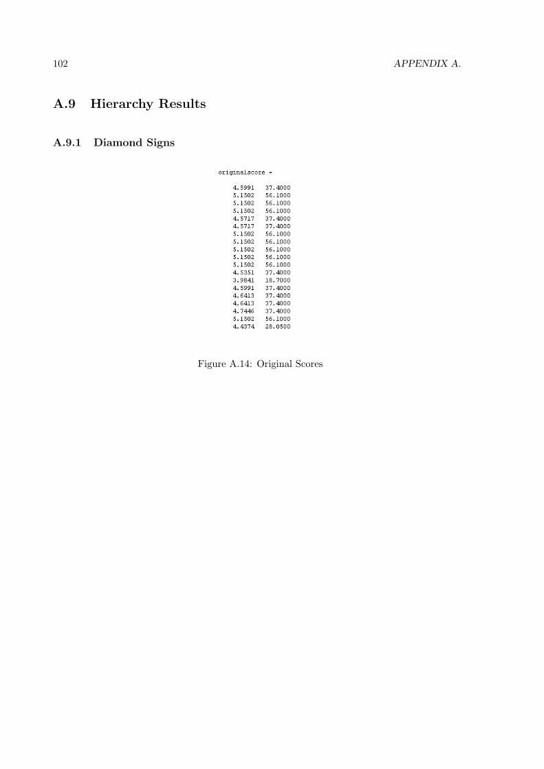
102 APPENDIX A.

A.9 Hierarchy Results

A.9.1 Diamond Signs

Figure A.14: Original Scores

A.9. HIERARCHY RESULTS 103

Figure A.15: Optimised Scores

104 APPENDIX A.

The following leaf level groupings were generated figures A.16-A.29.

Figure A.16: First Group

Figure A.17: First Group Template

Figure A.18: Second Group, template = self


Figure A.19: Third Group, template = self

Figure A.20: Fourth Group

Figure A.21: Fourth Group Template

106 APPENDIX A.

Figure A.22: Fifth Group

Figure A.23: Fifth Group Template

Figure A.24: Sixth Group


Figure A.25: Sixth Group Template

Figure A.26: Seventh Group

Figure A.27: Seventh Group Template

Figure A.28: Eigth Group

108 APPENDIX A.

Figure A.29: Eight Group Template


It is apparent from inspection of the groups that the optimisation is “sensible’. Though the

crossroad image has not been placed in a group with the left side road image, upon closer

inspection it can be seen that despite their likeness neither have similar features aligned with

the sign outline. By applying the same commands on the template images, the next level of the

hierarchy is generated.

The first grouping was of the 1st, 2nd and 4th groups (figure A.30).The second group was of the

3rd and 5th groups (figure A.32). The Crossroad sign was still “by itself” and the last grouping

was of the 7th and 8th groups (figure A.34).

Figure A.30: First Template Group

Figure A.31: First Template Group Combinational Template

110 APPENDIX A.

Figure A.32: Second Template Group

Figure A.33: Second Template Group Combinational Template

Figure A.34: Last Template Group

Figure A.35: Last Template Group Combinational Template


A.9.2 Circular Signs Scores

Figure A.36: Second Level Optimisation

112 APPENDIX A.

A.10 Matlab Matching Results

This is the original image (figure A.37), the oriented edge detection (figure A.38) and distance

transform (figure A.39).

Figure A.37: Original Image

Figure A.38: Oriented Edge Image

This diagram shows the scores achieved at points throughout the image. The unnecessary

expansion of the search over noisy areas of the edge detection can be seen (figures A.40 A.41)

A.10. MATLAB MATCHING RESULTS 113

Figure A.39: Distance Transform Image

and the match (figure A.42).

114 APPENDIX A.

Figure A.40: Scores

Figure A.41: Closer View of scores

Figure A.42: Match

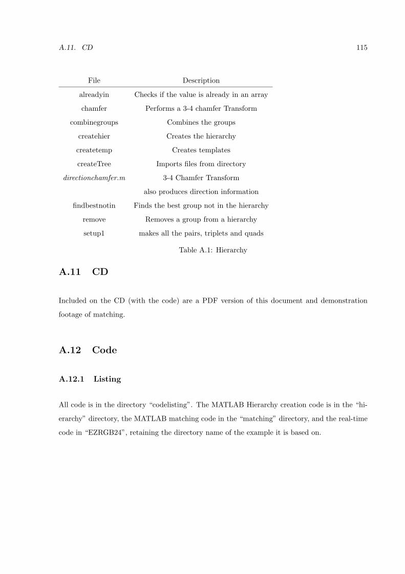
A.11. CD 115

File Description

alreadyin Checks if the value is already in an array

chamfer Performs a 3-4 chamfer Transform

combinegroups Combines the groups

createhier Creates the hierarchy

createtemp Creates templates

createTree Imports files from directory

directionchamfer.m 3-4 Chamfer Transform

also produces direction information

findbestnotin Finds the best group not in the hierarchy

remove Removes a group from a hierarchy

setup1 makes all the pairs, triplets and quads

Table A.1: Hierarchy

A.11 CD

Included on the CD (with the code) are a PDF version of this document and demonstration

footage of matching.

A.12 Code

A.12.1 Listing

All code is in the directory “codelisting”. The MATLAB Hierarchy creation code is in the “hi-

erarchy” directory, the MATLAB matching code in the “matching” directory, and the real-time

code in “EZRGB24”, retaining the directory name of the example it is based on.

116 APPENDIX A.

File Description

nonmaxsuppression Simple Non-maximal Suppression

R10Simplepyroverlay fine/coarse search using one template

overlay takes an image and a template

and simply translates the template across the image

simplepyrdirectedoverlay.m simple pyramid overlay with

edge direction

simplepyroverlay.m simplepyroverlay - simple finecoarse

overlaying

Table A.2: MATLAB Matching

File Description

EZRGB24 The Filter

mytree Abstract Builder for Trees

mytemplatev Template Class

mytreev A Concrete Builder

mytreel Another Concrete Builder

Table A.3: Real-Time

Hierarchy

MATLAB Matching

This code is “unfinished” hence only useful files are described.

Real-Time

Header files are also included. The file for creating templates (templatecreate.m) is in the “co-

existing” directory. Templates have been included in the “templates” directory under coexisting

but not described.

A.12. CODE 117

A.12.2 Compilation

Compilation of the Visual C++ code requires the installation of Microsoft’s DirectX SDK, IPL

Image Processing Library and OpenCV. The EZRGB24 example which this is based on needs

the baseclasses as referenced in the project settings. Include paths must be set. It must also

be able to find the *.lib files for IPL and OpenCV at compile and the appropriate *.dlls at

run time. See Brian Lovell’s ([email protected]) notes from ELEC4600 on compiling direct

show applications for more information. To run the code templates must be found (Hidden in

codelisting/templates/temps).

6281441-thesis

Documents