6. random variables

CSE 312, 2011 Winter, W.L.Ruzzo

random variables

23

numbered balls

24

Ross 4.1 ex 1b

first head

25

probability mass functions

26

Let X be the number of heads observed in n coin flips

Probability mass function:

head count

27

n = 2 n = 8

0 1 2

0.0

0.2

0.4

k

probability

0 1 2 3 4 5 6 7 8

0.0

0.2

0.4

k

probability

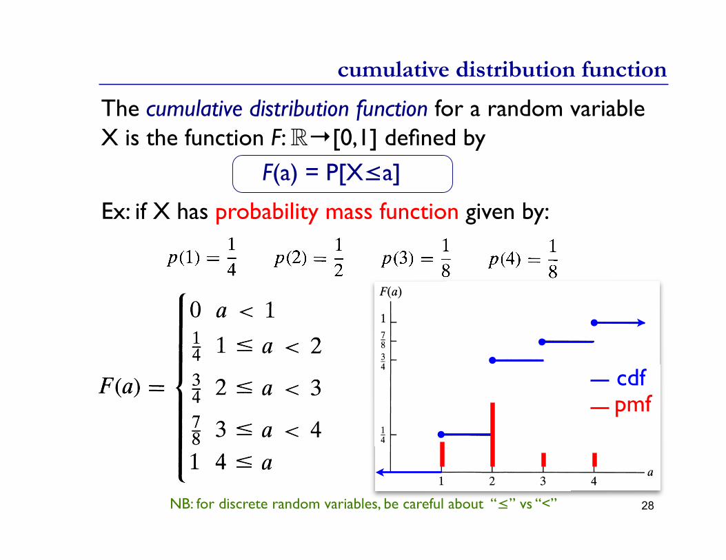
The cumulative distribution function for a random variable X is the function F: →[0,1] defined by

F(a) = P[X≤a]

Ex: if X has probability mass function given by:

cdfpmf

cumulative distribution function

28NB: for discrete random variables, be careful about “≤” vs “<”

expectation

29

. Long term net gain/loss = 0.

average of random values, weighted by their respective probabilities

30

first head

dy0/dy = 0

Calculating E[g(X)]:Y=g(X) is a new r.v. Calc P[Y=j], then apply defn:

X = sum of 2 dice rolls Y = g(X) = X mod 5

expectation of a function of a random variable

31

j q(j) = P[Y = j] j•q(j)-

0

1

2

3

4

4/36+3/36 =7/36 0/36-

5/36+2/36 =7/36 7/36-

1/36+6/36+1/36 =8/36 16/36-

2/36+5/36 =7/36 21/36-

3/36+4/36 =7/36 28/36-

72/36-

i p(i) = P[X=i] i•p(i)

2 1/36 2/36

3 2/36 6/36

4 3/36 12/36

5 4/36 20/36

6 5/36 30/36

7 6/36 42/36

8 5/36 40/36

9 4/36 36/36

10 3/36 30/36

11 2/36 22/36

12 1/36 12/36

252/36E[X] = Σi ip(i) = 252/36 = 7

E[Y] = Σj jq(j) = 72/36 = 2

Calculating E[g(X)]: Another way – add in a different order, using P[X=...] instead of calculating P[Y=...]

X = sum of 2 dice rolls Y = g(X) = X mod 5

expectation of a function of a random variable

32

j q(j) = P[Y = j] j•q(j)-

0

1

2

3

4

4/36+3/36 =7/36 0/36-

5/36+2/36 =7/36 7/36-

1/36+6/36+1/36 =8/36 16/36-

2/36+5/36 =7/36 21/36-

3/36+4/36 =7/36 28/36-

72/36-

i p(i) = P[X=i] g(i)•p(i)

2 1/36 2/36

3 2/36 6/36

4 3/36 12/36

5 4/36 0/36

6 5/36 5/36

7 6/36 12/36

8 5/36 15/36

9 4/36 16/36

10 3/36 0/36

11 2/36 2/36

12 1/36 2/36

72/36E[g(X)] = Σi g(i)p(i) = 252/3= 2

E[Y] = Σj jq(j) = 72/36 = 2

Above example is not a fluke.

Theorem: if Y = g(X), then E[Y] = Σi g(xi)p(xi), where xi, i = 1, 2, ... are all possible values of X.Proof: Let yj, j = 1, 2, ... be all possible values of Y.

expectation of a function of a random variable

33

xi6

xi1

xi3

X Yg

yj1

yj2

xi2

xi4

xi5

yj3

Note that Sj = { xi | g(xi)=yj } is a partition of the domain of g.

properties of expectation

34

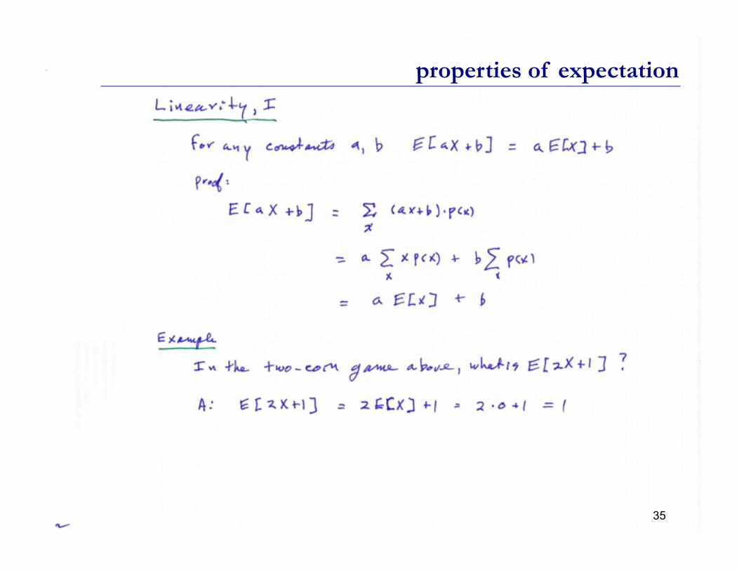
35

properties of expectation

36

properties of expectationRoss 4.9

True even ifX, Y dependentE[X+Y] = E[X] + E[Y]

E[X+Y] = E[Z] = Σs∈SZ[s] p(s) = Σs∈S(X[s] + Y[s]) p(s) = Σs∈SX[s] p(s) + Σs∈SY[s] p(s) = E[X] + E[Y]

37

properties of expectation

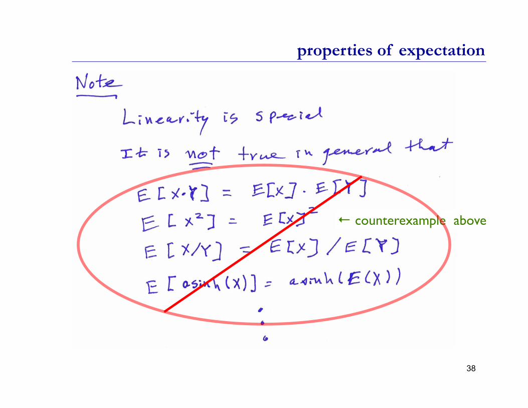
38

properties of expectation

← counterexample above

39

risk,

40

variance

41

risk,

mean and variance

μ = E[X] is about location; σ = √Var(X) is about spread

42

σ

σ

μ

μ

# heads in 20 flips, p=.5

# heads in 150 flips, p=.5

properties of variance

43

properties of variance

44

Example: What is Var(X) when X is outcome of one fair die?

E(X) = 7/2, so

Var[aX+b] = a2 Var[X]

Ex:

properties of variance

45

E[X] = 0Var[X] = 1

Y = 1000 X E[Y] = E[1000 X] = 1000 E[x] = 0Var[Y] = Var[1000 X] =106Var[X] = 106

a zoo of (discrete) random variables

46

bernoulli random variables

An experiment results in “Success” or “Failure”X is a random indicator variable (1=success, 0=failure) P(X=1) = p and P(X=0) = 1-pX is called a Bernoulli random variable: X ~ Ber(p)E[X] = pVar(X) = E[X2] – (E[X])2 = p – p2 = p(1-p)

Examples:coin fliprandom binary digitwhether a disk drive crashed

47

Jacob (aka James, Jacques) Bernoulli, 1654 – 1705

binomial random variables

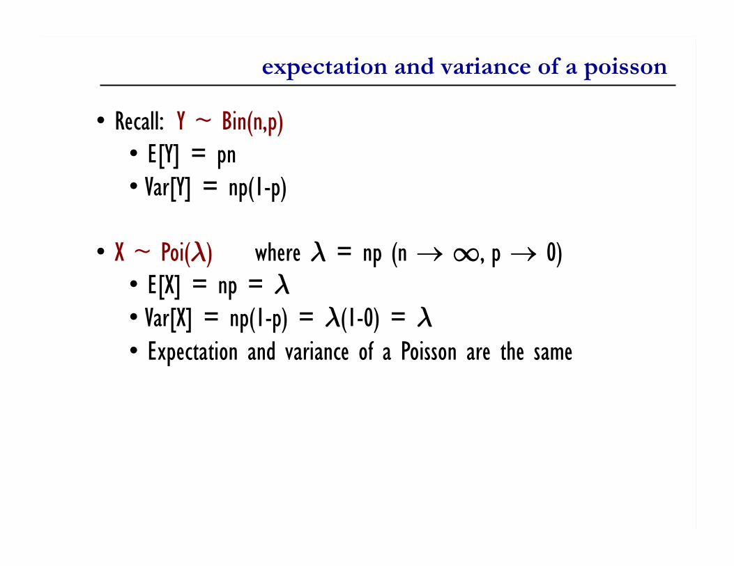
Consider n independent random variables Yi ~ Ber(p) X = Σi Yi is the number of successes in n trialsX is a Binomial random variable: X ~ Bin(n,p)

By Binomial theorem, Examples

# of heads in n coin flips# of 1’s in a randomly generated length n bit string# of disk drive crashes in a 1000 computer cluster

E[X] = pnVar(X) = p(1-p)n

48

←(proof below, twice)

binomial pmfs

49

0 2 4 6 8 10

0.00

0.05

0.10

0.15

0.20

0.25

0.30

PMF for X ~ Bin(10,0.5)

k

P(X=k)

µ ± !

0 2 4 6 8 10

0.00

0.05

0.10

0.15

0.20

0.25

0.30

PMF for X ~ Bin(10,0.25)

k

P(X=k)

µ ± !

binomial pmfs

50

0 5 10 15 20 25 30

0.00

0.05

0.10

0.15

0.20

0.25

PMF for X ~ Bin(30,0.5)

k

P(X=k)

µ ± !

0 5 10 15 20 25 30

0.00

0.05

0.10

0.15

0.20

0.25

PMF for X ~ Bin(30,0.1)

k

P(X=k)

µ ± !

using

k=1 gives:

hence:

letting j = i-1

mean and variance of the binomial

51

products of independent r.v.s

52

Note: NOT true in general; see earlier example E[X2]≠E[X]2

variance of independent r.v.s is additive

53

← recall Var(aX+b) = a2Var(X)

(Bienaymé, 1853)

Var

variance of independent r.v.s is additive

54

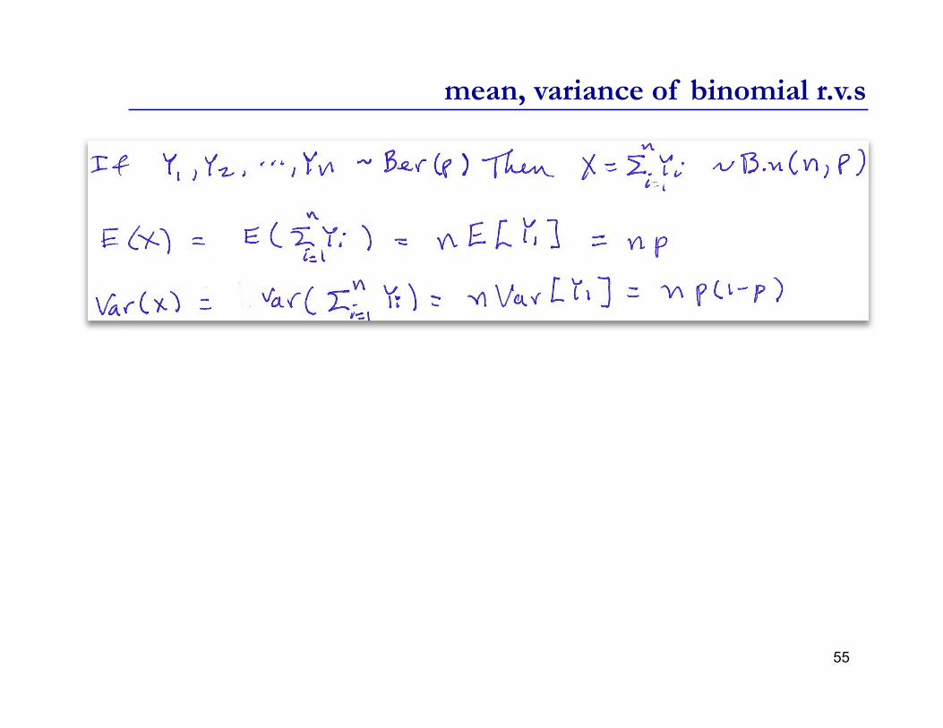
mean, variance of binomial r.v.s

55

disk failures

A disk array consists of n drives, each of which will fail independently with probability p.Suppose it can operate effectively if at least one-half of its components function, e.g., by “majority vote.”For what values of p is a 5-component system more likely to operate effectively than a 3-component system?

X5 = # failed in 5-component system ~ Bin(5, p)X3 = # failed in 3-component system ~ Bin(3, p)

56

Ross 4.6 ex 6f

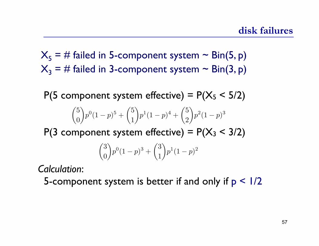
X5 = # failed in 5-component system ~ Bin(5, p) X3 = # failed in 3-component system ~ Bin(3, p)

P(5 component system effective) = P(X5 < 5/2)

P(3 component system effective) = P(X3 < 3/2)

Calculation: 5-component system is better if and only if p < 1/2

57

disk failures

error correcting codes

The Hamming(7,4) code:Have a 4-bit string to send over the network (or to disk)Add 3 “parity” bits, and send 7 bits totalIf bits are b1b2b3b4 then the three parity bits are parity(b1b2b3), parity(b1b3b4), parity(b2b3b4)Each bit is independently corrupted (flipped) in transit with probability 0.1X = number of bits corrupted ~ Bin(7, 0.1)

The Hamming code allow us to correct all 1 bit errors. (E.g., if b1 flipped, 1st 2 parity bits, but not 3rd, will look wrong; the only single bit error causing this symptom is b1. Similarly for any other single bit being flipped. Some multi-bit errors can be detected, but not corrected, but not arbitrarily many.)

P(correctable message received) = P(X=0) + P(X=1)

58

error correcting codes

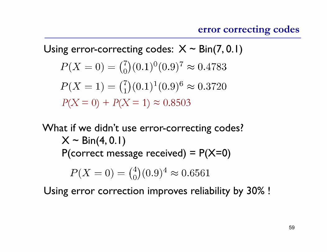
Using error-correcting codes: X ~ Bin(7, 0.1)

P(X = 0) + P(X = 1) ≈ 0.8503

What if we didn’t use error-correcting codes? X ~ Bin(4, 0.1) P(correct message received) = P(X=0)

Using error correction improves reliability by 30% !

59

models & reality

Sending a bit string over the networkn = 4 bits sent, each corrupted with probability 0.1X = # of corrupted bits, X ~ Bin(4, 0.1)In real networks, large bit strings (length n ≈ 104)Corruption probability is very small: p ≈ 10-6

X ~ Bin(104, 10-6) is unwieldy to computeExtreme n and p values arise in many cases

# bit errors in file written to disk # of typos in a book# of elements in particular bucket of large hash table # of server crashes per day in giant data center# facebook login requests sent to a particular server

60

61

!"#$$"%&'(%)"*&+('#(,-.

!"#$"%"&'#$$'( )%(*'+",%)#%-./0""!"1"&'#2!3

%(*4"5')"%"6#,/("7%)%+/8/)"!49%$"*#$8)#-:8#'("2&;<30

='8/">%?.')"$/)#/$0

Siméon Poisson, 1781-1840

62

!"#$$"%&'(%)"*&+('#(,-.&#$&,#%"*#(-&#%&/0.&-#*#/

!"#$$"%&'(()"*#+',-$&.#%"+#'/&01-%&%&#$&/')2-3&(&#$&$+'//3'%4&! 5&%(

%&6&78&'%4&(&9&8:8;%&6&<88&'%4&(&9&8:<

=")+'//>3&!"#$$"%&#$&?#%"+#'/&'$%& ! '%4&(& 83&01-)-&%( 5&!

binomial → poisson in the limit

63

64

!"#$%#&'$()('*#'('#")+*,-.'(&(%#

!"#$%%&"'$()%"&*+&,"-./-0&1/2&,23/-0&*4"3&$&-"25*367"-.&1/2&,23/-0&*+&%"-028&-&9&10:;3*1$1/%/2<&*+&=/-.")"-."-2>&1/2&#*33?)2/*-&/,&)&9&10@AB&C&;*/=! 9&10:!10@A 9&DEDF>G8$2&/,&)3*1$1/%/2<&28$2&(",,$0"&$33/4",&?-#*33?)2".H

I,/-0&J&C&K/-(10:L&10@A>M

;=J9D>&" DENNDD:NOPN

65

66

!"#!$%&%'()*&)+*,&-'&)$!*(.*&*#('//()

!"#$%%&''(')'*+,-,./012(3'4'/,5$62(3'4',/-78/0

9')':;+-!0 <="6"'! 4',/ -,' !.'/' >01293'4',/ 4'!5$6293'4',/-78/0'4'!-78>0'4'!1?/"#@$@+;,'$,A'B$6+$,#"';C'$':;+DD;,'$6"'@="'D$E"

F;6"':;+DD;,',"?@'@+E"G

buffers

Suppose a server can process 2 requests per secondRequests arrive at random at an average rate of 1/sec Unprocessed requests are held in a buffer Q. How big a buffer do we need to avoid ever dropping a request?A. InfiniteQ. How big a buffer do we need to avoid dropping a request more often than once a day?A. (approximate) If X is the number of arrivals in a second, then X is poisson(λ=1). We want b s.t. P(X > b) < 1/(24*60*60) ≈ 10-5

P(X = b) = e-1/b! P(X=8) ≈ Σi>7 P(X=i) ≈ 1.02e-05

67

balls in urns – the hypergeometric distribution

Draw d balls (without replacement) from an urn containing N, of which w are white, the rest black. Let X = number of white balls drawn

(note: n choose k = 0 if k < 0 or k > n)

E[X] = dp, where p = w/N (the fraction of white balls)proof: Let Xi be 0/1 indicator for i-th ball is white, X = Σ Xi

The Xi are dependent, but E[X] = E[Σ Xi] = Σ E[Xi] = dp

Var[x] = dp(1-p)(1-(d-1)/(N-1))

68

N

d

data mining

N ≈ 22500 human genes, many of unknown functionSuppose in some experiment, d =1588 of them were observed (say, they were all switched on in response to some drug)

A big question: What are they doing?

One idea: The Gene Ontology Consortium (www.geneontology.org) has grouped genes with known functions into categories such as “muscle development” or “immune system.” Suppose 26 of your d genes fall in the “muscle development” category.

Just chance?Or call Coach & see if he wants to dope some athletes?

Hypergeometric: GO has 116 genes in the muscle development category. If those are the white balls among 22500 in an urn, what is the probability that you would see 26 of them in 1588 draws?

69

data mining

70

A differentially bound peak was associated to the closest gene (unique Entrez ID) measured by distance to TSS within CTCF flanking domains. OR: ratio of predicted to observed number of genes within a given GO category. Count: number of genes with differentially bound peaks. Size: total number of genes for a given functional group. Ont: the Geneontology. BP = biological process, MF = molecular function, CC = cellular component.

Cao, et al., Developmental Cell 18, 662–674, April 20, 2010

probability of seeing this many genes from a set of this size by chance according to

the hypergeometric distribution. E.g., if you draw 1588 balls from an urn containing 490 white balls

and ≈22000 black balls, P(94 white) ≈2.05×10-11