6. antarcticar. l. fogt and s. stammerjohn, eds. tively...

6. ANTARCTICA—R. L. Fogt and S. Stammerjohn, Eds.a. Overview—R. L. Fogt and S. Stammerjohn

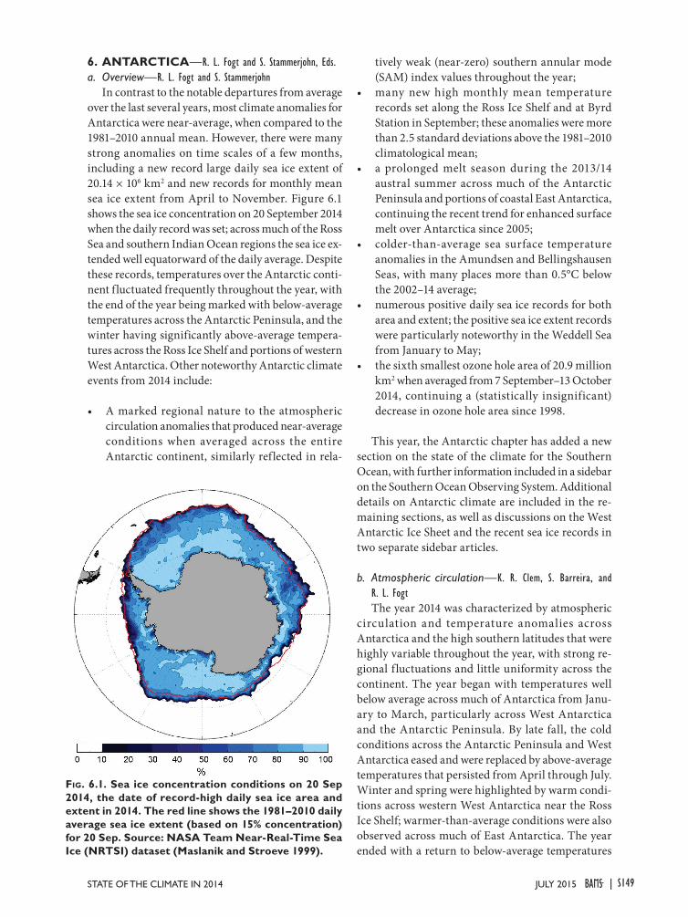
In contrast to the notable departures from average over the last several years, most climate anomalies for Antarctica were near-average, when compared to the 1981–2010 annual mean. However, there were many strong anomalies on time scales of a few months, including a new record large daily sea ice extent of 20.14 × 106 km2 and new records for monthly mean sea ice extent from April to November. Figure 6.1 shows the sea ice concentration on 20 September 2014 when the daily record was set; across much of the Ross Sea and southern Indian Ocean regions the sea ice ex-tended well equatorward of the daily average. Despite these records, temperatures over the Antarctic conti-nent fluctuated frequently throughout the year, with the end of the year being marked with below-average temperatures across the Antarctic Peninsula, and the winter having significantly above-average tempera-tures across the Ross Ice Shelf and portions of western West Antarctica. Other noteworthy Antarctic climate events from 2014 include:

• A marked regional nature to the atmospheric circulation anomalies that produced near-average conditions when averaged across the entire Antarctic continent, similarly reflected in rela-

tively weak (near-zero) southern annular mode (SAM) index values throughout the year;

• many new high monthly mean temperature records set along the Ross Ice Shelf and at Byrd Station in September; these anomalies were more than 2.5 standard deviations above the 1981–2010 climatological mean;

• a prolonged melt season during the 2013/14 austral summer across much of the Antarctic Peninsula and portions of coastal East Antarctica, continuing the recent trend for enhanced surface melt over Antarctica since 2005;

• colder-than-average sea surface temperature anomalies in the Amundsen and Bellingshausen Seas, with many places more than 0.5°C below the 2002–14 average;

• numerous positive daily sea ice records for both area and extent; the positive sea ice extent records were particularly noteworthy in the Weddell Sea from January to May;

• the sixth smallest ozone hole area of 20.9 million km2 when averaged from 7 September–13 October 2014, continuing a (statistically insignificant) decrease in ozone hole area since 1998.

This year, the Antarctic chapter has added a new section on the state of the climate for the Southern Ocean, with further information included in a sidebar on the Southern Ocean Observing System. Additional details on Antarctic climate are included in the re-maining sections, as well as discussions on the West Antarctic Ice Sheet and the recent sea ice records in two separate sidebar articles.

b. Atmospheric circulation—K. R. Clem, S. Barreira, and

R. L. FogtThe year 2014 was characterized by atmospheric

circulation and temperature anomalies across Antarctica and the high southern latitudes that were highly variable throughout the year, with strong re-gional fluctuations and little uniformity across the continent. The year began with temperatures well below average across much of Antarctica from Janu-ary to March, particularly across West Antarctica and the Antarctic Peninsula. By late fall, the cold conditions across the Antarctic Peninsula and West Antarctica eased and were replaced by above-average temperatures that persisted from April through July. Winter and spring were highlighted by warm condi-tions across western West Antarctica near the Ross Ice Shelf; warmer-than-average conditions were also observed across much of East Antarctica. The year ended with a return to below-average temperatures

Fig. 6.1. Sea ice concentration conditions on 20 Sep 2014, the date of record-high daily sea ice area and extent in 2014. The red line shows the 1981–2010 daily average sea ice extent (based on 15% concentration) for 20 Sep. Source: NASA Team Near-Real-Time Sea Ice (NRTSI) dataset (Maslanik and Stroeve 1999).

S149JULY 2015STATE OF THE CLIMATE IN 2014 |

across the Antarctic Peninsula and portions of West Antarctica, while the rest of the continent experi-enced near-average temperatures.

The circulation and temperature anomalies are examined in detail in Figs. 6.2 and 6.3, based on the ERA-Interim reanalysis data (Dee et al. 2011a). The year was split into four periods (indicated by red verti-cal lines in Fig. 6.2), based on when monthly spatial temperature and pressure anomalies were persistent and of similar sign, taking into account the highly regional behavior of the atmosphere during 2014. The composite anomalies (contours) and standard

deviation of the anomalies from the 1981–2010 cli-matological mean (shading) for these periods are presented in Fig. 6.3.

The year began with near-average geopotential height poleward of 60°S during January–March (Fig. 6.2a), with weakly negative geopotential height anomalies between 500 hPa and 300 hPa during February. This is also evident in the surface pressure (SP) anomalies from January to March in Fig. 6.3a, with the dominant regional circulation feature being a strong positive SP anomaly (4–5 hPa, 2–3 standard deviations above the climatological average) in the

Fig. 6.2. Area-weighted averaged climate parameter anomalies for the southern polar region in 2014 relative to 1981–2010: (a) polar cap (60°–90°S) averaged geopo-tential height anomalies (50-m contour interval, with additional contour at ± 25 m); (b) polar cap averaged temperature anomalies (1°C contour interval, with ad-ditional contour at ± 0.5°C); (c) circumpolar (50°–70°S) averaged zonal wind anomalies (2 m s–1 contour inter-val, with additional contour at ± 1 m s–1). Shading rep-resents standard deviation of the anomalies from the 1981–2010 mean. (Source: ERA-Interim reanalysis.) Red vertical bars indicate the four separate climate periods used for compositing in Fig. 6.3; the dashed lines near Dec 2013 and Dec 2014 indicate circulation patterns wrapping around the calendar year. Values for the CPC SAM index are shown along the bottom in black (positive values) and red (negative values).

Fig. 6.3. (left) Surface pressure anomalies and (right) 2-m temperature anomalies relative to 1981–2010 for (a) and (b) Jan–Mar 2014; (c) and (d) Apr–Jul 2014; (e) and (f) Aug–Sep 2014; (g) and (h) Oct–Dec 2014. Con-tour interval for (a), (c), (e), and (g) is 2 hPa; contour interval for (b) and (h) is 1°C and for (d) and (f) 2°C. Shading represents standard deviations of anomalies relative to the relevant season of the 1981–2010 mean. (Source: ERA-Interim reanalysis.)

S150 JULY 2015|

South Pacific at ~50°S (Fig. 6.3a). Nearby, negative temperature anomalies of more than 1°–2°C (>2.5 standard deviations; Fig. 6.3b) occurred across West Antarctica and the Antarctic Peninsula. Figure 6.2b shows that temperatures averaged over the polar cap were also below average throughout the lower half of the troposphere from mid-January through March. The circumpolar zonal winds (Fig. 6.2c) were above average from February to March, beginning first at ~75 hPa during February and propagating down through the troposphere during March.

During the late fall/early winter (April–July) period, the atmospheric circulation around Antarc-tica was strongly meridional (Fig. 6.3c). Negative SP anomalies were present across much of the high-lati-tude South Pacific (indicating an increase in low pres-sure occurrence west of the Antarctic Peninsula) while positive SP anomalies were located in the South Atlan-tic and off the east coast of New Zealand (Fig. 6.3c). This atmospheric circulation caused large regional temperature anomalies. In particular, the April–July period was marked with above-average temperatures across the Antarctic Peninsula and eastern West Ant-arctica (>1 standard deviation), and below-average temperatures over extreme western West Antarctica near the Ross Ice Shelf and extending out over the Ross and Amundsen Seas (>2 standard deviations; Fig. 6.3d). Turning to Fig. 6.2a, geopotential height anomalies averaged poleward of 60°S were weak and primarily <1 standard deviation from climatology during the April–July period, reflecting the regional nature of the anomaly patterns in Fig. 6.3c,d. An in-crease in the magnitude of the circumpolar-averaged zonal winds developed during June (Fig. 6.2c), with positive zonal wind anomalies throughout the tropo-sphere and stratosphere during this month, the most significant being located above 50 hPa (>1.5 standard deviations). Last, the April–July period began with strong positive temperature anomalies poleward of 60°S between 300 hPa and 200 hPa (+1°C; >2 standard deviations; Fig. 6.2b), which developed in February and persisted/intensified through March and April, before finally weakening after May.

The regional atmospheric circulation anomalies changed once again during the August–September period. From Fig. 6.3e, the most prominent circu-lation anomalies inf luencing West Antarctica are positive SP anomalies over the Antarctic Peninsula and negative SP anomalies in the Ross Sea (along and east of the dateline). Associated with these two circulation anomalies were large positive temperature anomalies across western West Antarctica and over the Ross Ice Shelf (>6°C and >3 standard deviations)

and cold temperature anomalies over the South-ern Ocean west of 150°W (>2 standard deviations; Fig. 6.3f). Across East Antarctica, weak positive SP anomalies dominated most of the ice sheet during August–September (Fig. 6.3e) and, for the most part, temperatures were near-average to slightly above aver-age. Averaged poleward of 60°S, August–September was dominated by weak positive geopotential height anomalies throughout the troposphere and strato-sphere, the most significant located in the troposphere during September (Fig. 6.2a). The polar cap-averaged temperature anomalies were near zero due to the can-celling effect of strong positive and negative regional anomalies in Fig. 6.3f; however, the troposphere and stratosphere were altogether warmer than average (Fig. 6.2b). Circumpolar zonal winds were also near-average over the period, with slightly weaker-than-average zonal winds observed during September when the region south of 60°S reached its strongest positive SP anomaly and the SAM index reached −1.12.

The last quarter of 2014 started with near-average SP and temperatures across most of Antarctica from October to December (Fig. 6.3g,h). The only excep-tion was the Antarctic Peninsula, which saw colder-than-average temperatures (Fig. 6.3h) due to the development of negative SP anomalies in the South Atlantic and positive SP anomalies in the South Pa-cific, which collectively led to increased cold, offshore f low across the Peninsula. In December, the most pronounced nonregional circulation pattern of the year emerged, with negative pressures/heights across the Antarctic continent, stronger-than-average cir-cumpolar zonal winds, and the largest positive SAM index (+1.32) of the year (Fig. 6.2).

c. Surface staffed and automatic weather station observations—S. Colwell, L. M. Keller, M. A. Lazzara, A. Setzer, and R. L. FogtThe circulation anomalies described in section 6b

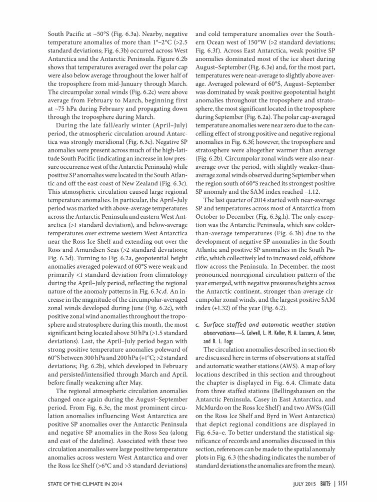
are discussed here in terms of observations at staffed and automatic weather stations (AWS). A map of key locations described in this section and throughout the chapter is displayed in Fig. 6.4. Climate data from three staffed stations (Bellingshausen on the Antarctic Peninsula, Casey in East Antarctica, and McMurdo on the Ross Ice Shelf) and two AWSs (Gill on the Ross Ice Shelf and Byrd in West Antarctica) that depict regional conditions are displayed in Fig. 6.5a–e. To better understand the statistical sig-nificance of records and anomalies discussed in this section, references can be made to the spatial anomaly plots in Fig. 6.3 (the shading indicates the number of standard deviations the anomalies are from the mean).


At the north of the Antarctic Peninsula, a record low (since observations began in 1969) monthly mean temperature of −0.1°C was observed at Bellingshausen in February (anomaly shown in Fig. 6.5a); record-high wind speeds were recorded at Bellingshausen in No-vember, 1.82 m s−1 above the mean (Bellingshausen meteorological data starts in 1968). Monthly mean temperatures at Rothera Station on the western side of the Antarctic Peninsula were similar to their respective 1981–2010 averages, with temperatures slightly below average during the summer months and slightly above average during the winter months. The lower-than-average temperatures at the north-ern Antarctic Peninsula continue a recent trend of cooling in this region, as reflected in Fig. 6.5f, where

austral summer temper-ature changes over 1976–2013 are shown for four stations with the long-est and most complete records. W hi le many stations at the northern Antarctic Peninsula ob-served a warming trend in the early part of their records, there has been a stat ist ica l ly signif i-cant cooling of p < 0.10 at all but Faraday since 1995 (dashed l ines in Fig. 6.5f; the trends range from −0.03°C decade−1 at Faraday to −0.73°C decade−1 at Bellingshaus-en and Marambio dur-ing December–Febru-ary 1995/96–2013/14). Despite the short period of these recent negative trends, they do indicate a weakening of the positive trends over the last 20 years (see also Colwell et al. 2014; McGrath and Steffen 2012).

In the nearby Weddell Sea region (not shown), the monthly mean tem-peratures at Halley and Neumayer stations were near-average year-round with two exceptions: 1) April at Neumayer, where

Fig. 6.4. Map of stations and other regions used throughout the chapter.

Fig. 6.5. (a)–(e) 2014 Antarctic climate anomalies at five representative stations [three staffed (a)–(c), and two automatic (d)–(e)]. Monthly mean anomalies for temperature (°C), MSLP (hPa), and wind speed (m s–1) are shown, + denoting record anomalies for a given month at each station in 2014 and * denoting tied records in 2014. All anomalies are based on differences from 1981–2010 averages, except for Gill, which is based on averages during 1985–2013. (f) Austral summer (Dec–Feb) mean observed temperatures for stations at the northern Antarctic Peninsula, 1976–2013. Also shown are linear trends from 1995–2013. The year on the ordinate axis represents the Dec of each summer season.

S152 JULY 2015|

the monthly mean temperature of −22.0°C tied the record low previously set in April 2007; and 2) in early August at Halley, where a new daily extreme minimum temperature of −55.4°C was recorded.

Around the coast of East Antarctica, all of the Australian stations (Mawson, Davis, Casey) had some months with temperatures above and below average, with Casey (Fig. 6.5b) and Mawson showing similar differences from the long-term mean. All three sta-tions observed record or near-record high monthly mean temperature values for November (Casey −3.7°C; Davis −2.5°C; Mawson −4.0°C). Casey expe-rienced high winds in September with gusts of up to 64 m s−1 recorded on one day, leading to a new record high monthly September wind speed (Fig. 6.5b).

During 2014, much of the interior of the Antarctic continent started out with below-average tempera-tures during austral summer, followed by above-av-erage temperatures during austral fall through spring, as seen in Fig. 6.3. At Amundsen Scott Station, for example, lower-than-average monthly mean temper-atures were recorded during February and March, followed by higher-than-average temperatures during April, May, and June. Dome C II in East Antarctica had lower-than-average temperature, pressure, and wind speed for most of the year, especially in June, July, and August.

Many records were reported throughout the year for the Ross Ice Shelf and West Antarctica (Fig. 6.5c–e). Due to the circulation anomalies (dis-cussed in section 6b), the Ross Ice Shelf and vicinity saw many extremes recorded in August and Septem-ber (Fig. 6.3f). Record high monthly mean tempera-tures were observed in August at Gill (+11.6°C above the mean; Fig. 6.5d), a tied record high at Possession Island (−16.2°C, +4.5°C above the 1993–2013 mean for this station), and near-record temperatures at Marble Point (+6.1°C above the mean) and Byrd (+7.2°C above the mean). In September, record high monthly temperatures were reported at McMurdo (+6.2°C above the mean; Fig. 6.5c), Gill (+8.6°C above the mean; Fig. 6.5d), Marble Point (+6.9°C above the mean), and Byrd (+9.3°C above the mean; Fig. 6.5e). Many of these anomalies in August and September were more than 2 standard deviations above the long-term mean (Fig. 6.3f). Record low pressure and record high wind speed for August were also observed at Gill (−12.1 hPa below the mean and +3.2 m s−1 above the mean, respectively; Fig. 6.5d). In November and December, lower-than-average temperatures were observed at Byrd and Gill (Fig. 6.5d,e), which are par-tially reflected in the negative temperature anomalies across eastern West Antarctica in Fig. 6.3h (although

not over the Ross Ice Shelf when averaged from Oc-tober to December). Record temperatures for Byrd were 4.5°C and 4.1°C below the mean for November and December, respectively. For Gill, near-record and record temperatures were 2.7°C and 2.1°C below the mean in November and December, respectively.

Other months also set records for the Ross Ice Shelf area and West Antarctica. The highest January mean temperature was reported at Possession Island (+2.0°C above the mean) along with a near record for Marble Point (+2.2°C above the mean). Additional records were set at Byrd for high mean wind speed during January (2.0 m s−1 above the mean) and a tie for May (2.2 m s−1 above the mean; Fig. 6.5e). Gill also tied record high wind speeds for February and March, (0.9 and 1.0 m s−1 above the mean, respectively; Fig. 6.5d). In terms of pressure, in addition to the record lowest pressure observed at Gill in August (as mentioned above), record low pressure was also observed at Byrd in April 2014 (10.7 hPa below the mean), with well-below-average pressure also reported for June and July.

d. Net precipitation (P – E)—D. H. Bromwich and S.-H. WangPrecipitation minus evaporation/sublimation

(P – E) closely approximates the surface mass balance over Antarctica, except for the steep coastal slopes (e.g., Bromwich et al. 2011; Lenaerts and van den Broeke 2012). Precipitation variability is the domi-nant term for P – E changes at regional and larger scales over the Antarctic continent. Precipitation and evaporation/sublimation fields from ERA-Interim (Dee et al. 2011a) were examined to assess Antarctic net precipitation (P – E) behavior for 2014.

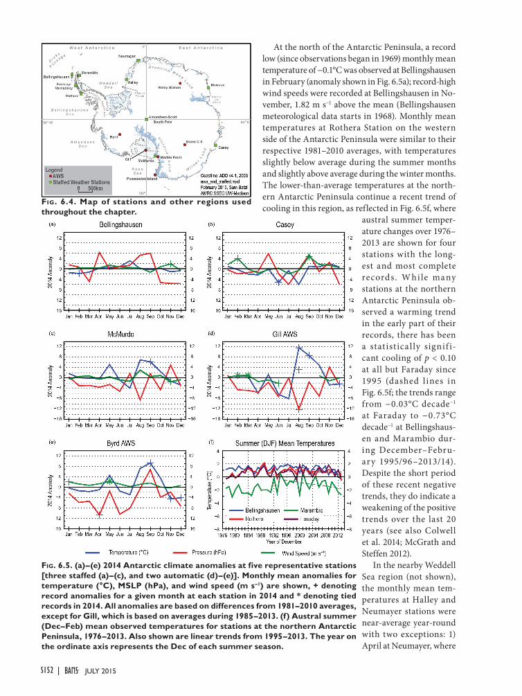
Figure 6.6 (a–d) shows the ERA-Interim 2014 and 2013 annual anomalies of P – E and mean sea level pressure (MSLP) departures from the 1981–2010 av-erage. In general, the magnitude of the annual P – E anomalies (Fig. 6.6a,b) ref lect the steep gradients between low annual snow accumulations within the continental interior to much larger annual accumula-tions near the Antarctic coastal regions. Compared to the 2013 Japanese reanalysis (JRA) P – E result from Bromwich and Wang (2014), both ERA-Interim and JRA show quantitative similarity at higher latitudes (poleward of 60°S). However, JRA has excessively high positive anomalies north of 60°S. Regardless, cau-tion should be exercised when examining the exact magnitudes of precipitation from global reanalyses in the high southern latitudes (Nicolas and Bromwich 2011); the main goal here is to demonstrate how these anomalies are qualitatively tied to changes in the atmospheric circulation.


From ERA-Interim, the negative P – E anoma-lies south of 60°S between 60° and 150°W in 2013 have been replaced by positive anomalies in 2014, especially along the Amundsen Sea coast. The ob-served negative anomalies over the Ross Sea have switched to weak positive ones. The annual P – E anomaly triplet (negative–near-average–negative) between Wilkes Land and Victoria Land (between 90° and 170°E) present in 2013 is nearly all negative in

2014. The P – E anoma-lies near the Amery Ice Shelf (between 50° and 80°E) switch from posi-tive (in 2013) to negative (in 2014). The positive P – E anomaly center over the Weddell Sea in 2013 has been replaced by a negative anomaly in 2014. Both sides of the Antarctic Peninsula have opposite anomaly pat-terns to 2013, with nega-tive (positive) anomalies along east (west) side of the peninsula in 2014.

These annual P – E anomaly features are generally consistent with the mean atmospheric circulation implied by the MSLP anomalies (Fig. 6.6c,d). In 2014, the annual MSLP anomalies surrounding Antarc-tica are generally more spatially uniform than in 2013 (due perhaps to the large variability in the location of the pat-terns during the year, as discussed in section 6b and in Fig. 6.3). The large negative anomaly center in 2013 over the Drake Passage and the Bellingshausen Sea (be-tween 45° and 120°W) is weaker and shifted to the Amundsen and Ross Seas in 2014. The atmospheric circulation in 2014 produced stron-

ger offshore f low (less precipitation) over Victoria Land, and stronger inflow (more precipitation) over West Antarctica between 60° and 150°W (Fig. 6.6a), from an annual mean standpoint. A positive MSLP anomaly center observed along the Queen Mary Coast (between 85° and 105°E) during 2013 was not present in 2014. Instead there is a strong negative anomaly center in the southern Indian Ocean (near 105°E) and weak positive anomalies along the coast

Fig. 6.6. P – E anomalies (mm) for (a) 2014 and (b) 2013; (c) MSLP anomalies (hPa) for (c) 2014 and (d) 2013. (Source: ERA-Interim reanalysis.) All anomalies are departures from the 1981–2010 mean. (e) Monthly total P – E (mm; dashed red) for the West Antarctic sector bounded by 75°–90°S, 120°W–180°, along with the SOI (dashed blue, from Climate Prediction Center) and SAM [dashed green, from Marshall (2003)] indices since 2010. Centered annual running means are plotted as solid lines (indicated in legend with “_12”).

S154 JULY 2015|

of East Antarctica. The 2014 circulation pattern in this area resulted in less precipitation (greater nega-tive P – E anomaly) in the coastal region between 60° and 180°E (than during 2013). The positive MSLP anomaly over the coast of Dronning Maud Land (from 15°W to 30°E) in 2013 has shifted to the southwest and strengthened in 2014. This resulted in enhanced blocking and less inf low, producing lower precipitation anomalies in the Weddell Sea region in 2014.

Earlier studies show that almost half of the mois-ture transport into Antarctica occurs in the West Antarctic sector and experiences large interannual variability associated with ENSO (e.g., Bromwich et al. 2004) and SAM events (e.g., Fogt et al. 2011). As the seasons progressed from 2013 to 2014, the nega-tive MSLP anomalies over the Ross Sea expanded into the Bellingshausen Sea and disappeared in spring of 2014 (see Fig. 6.3g). These anomaly features are con-sistent with a simultaneous weakening of La Niña and strengthening of SAM (from more negative to more positive phases). Figure 6.6e shows the time series of monthly average total P – E over Marie Byrd Land–Ross Ice Shelf (75°–90°S, 120°W–180°) and the monthly Southern Oscillation (SOI) and SAM indices (with 12-month running means). Qualitatively, it is clear that SOI and SAM are positively correlated, but are negatively cor-related with P – E in most months from 2010 to mid-2011. From then on the SOI is negatively correlated with the SAM into 2014. During 2013 into 2014, weak ENSO events prevailed in the tropical Pacific Ocean, and as such the SOI was near zero during that period. Thus, the wind patterns associated with positive SAM phases become the dominant factor modulating pre-cipitation into the West Antarctic sector, especially during the sec-ond half of 2014.

e. 2013/14 seasonal melt extent and duration—L. Wang, H. Liu, S. Wang, and S. ShuSea sona l su r face melt on

the Antarctic continent during 2013/14 has been estimated by using the daily measurements of microwave brightness temperature data acquired by the Defense Me-

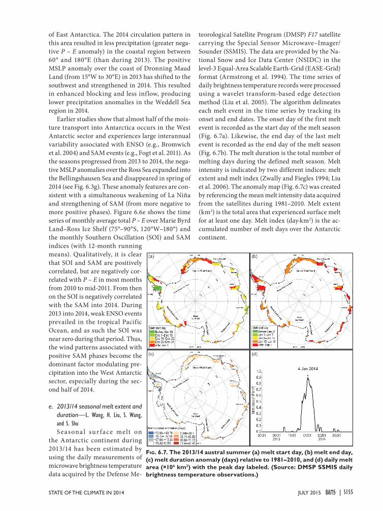
teorological Satellite Program (DMSP) F17 satellite carrying the Special Sensor Microwave–Imager/Sounder (SSMIS). The data are provided by the Na-tional Snow and Ice Data Center (NSIDC) in the level-3 Equal-Area Scalable Earth-Grid (EASE-Grid) format (Armstrong et al. 1994). The time series of daily brightness temperature records were processed using a wavelet transform-based edge detection method (Liu et al. 2005). The algorithm delineates each melt event in the time series by tracking its onset and end dates. The onset day of the first melt event is recorded as the start day of the melt season (Fig. 6.7a). Likewise, the end day of the last melt event is recorded as the end day of the melt season (Fig. 6.7b). The melt duration is the total number of melting days during the defined melt season. Melt intensity is indicated by two different indices: melt extent and melt index (Zwally and Fiegles 1994; Liu et al. 2006). The anomaly map (Fig. 6.7c) was created by referencing the mean melt intensity data acquired from the satellites during 1981–2010. Melt extent (km2) is the total area that experienced surface melt for at least one day. Melt index (day·km2) is the ac-cumulated number of melt days over the Antarctic continent.

Fig. 6.7. The 2013/14 austral summer (a) melt start day, (b) melt end day, (c) melt duration anomaly (days) relative to 1981–2010, and (d) daily melt area (×106 km2) with the peak day labeled. (Source: DMSP SSMIS daily brightness temperature observations.)


SIDEBAR 6.1: WAIS-TING AWAY? THE PERILOUS STATE OF THE WEST ANTARCTIC ICE SHEET—R. B. ALLEY

Accelerating mass loss from the West Antarctic Ice Sheet (WAIS) is of special concern. New work suggests that the full distribution of possible behaviors includes faster sea level rise than usually was previously considered, although with large uncertainties.

Glaciers and ice sheets generally shrink with warming, contributing to sea level rise, despite the usual increase in precipitation from warmer air supplying more water vapor (for a longer review, refer to Alley et al. 2015, in press). Mountain glaciers contain only ~0.4 m of sea level equivalent (SLE; Vaughan et al. 2013) and models indicate that shrinkage of the Greenland Ice Sheet (~7 m SLE) will have a multicentennial response time even for large warm-ing (Applegate et al. 2014), whereas the East Antarctic Ice Sheet (>50 m SLE) is less sensitive to initial atmospheric warming than the other ice masses. Large, abrupt sea level rise remains possible from the WAIS (~3.3 m SLE in marine portions; NRC 2013).

Most West Antarctic ice discharges across grounding lines into floating-but-attached ice shelves, which lose mass by basal melting and iceberg calving. Ice thinning at the grounding line causes it to migrate inland, but the bed generally deepens inland, allowing faster ice spreading, further thinning, and potentially unstable retreat. The most important stabilizer is friction between ice shelves and embayment sides or local sea-floor highs. Meltwater wedging from surface warming can disintegrate an ice shelf in weeks (e.g., Rott et al. 1996) and warmer waters

typically increase sub-ice-shelf melting by order 10 m yr–1 °C–1 (e.g., Rignot and Jacobs 2002), with 1°C warming or less sufficient to largely or completely remove many ice shelves.

Recently, ocean warming plus changing winds and, therefore, ocean circulation from some combination of the ozone hole, warming due to greenhouse gas increases, and natural variability (Schmidtko et al. 2014) have in-creased melting beneath the Amundsen Sea ice shelves facing the Pacific Ocean, causing ice-flow acceleration and thinning that dominate Antarctic mass loss (e.g., Sut-terly et al. 2014). Some but not all model results suggest that the threshold for irreversible but probably delayed retreat has already been crossed (Joughin et al. 2014; Parizek et al. 2013).

The paleoclimatic record in and around the ice sheet, and the far-field record of sea level, suggest but do not prove that the ice sheet shrank and likely disappeared one or more times within the last million years, for reasons including response to the rather small additional forcing of the last interglacial (Alley et al. 2015, in press). The far-field record of sea level indicators such as the distribution of well-dated marine deposits now above sea level (e.g., O’Leary et al. 2013), allows inferred deglaciation of West Antarctica to have required centuries or longer, but does not rule out ice loss over shorter times.

The rate of any future “collapse” may depend on the ice cliff dynamics of a “tidewater” glacier. When termi-

This year’s melt can be characterized by its exten-sive melt extent and an anomalously long melt season around most of coastal Antarctica except in the pen-insula and Abbot areas where both positive and nega-tive melt duration anomalies were observed (Fig. 6.7). Areas with intensive melt (>45 day duration) include areas of the Larsen and Wilkins ice shelves along the Antarctic Peninsula, the West and Shackleton ice shelves, and Wilkes Land in coastal East Antarctica. Areas with moderate intensity of melt (14–45 day duration) include much of coastal Queen Maud Land and the Abbot and Amery ice shelves; short-term melt (<14 day duration) occurred on the coast of Marie Byrd Land and portions of Queen Maud Land near the Filchner Ice Shelf. Although the melt duration anomaly was negative in most areas of the Antarctic Peninsula and Wilkins Ice Shelf (Fig. 6.7c) consistent with cooler than normal air temperature (see Fig. 6.3b), an anomalously early melt event (around 1 October 2013) was observed in these areas

(Fig. 6.7a). This melt event only lasted for less than a week however (Fig. 6.7d). Positive melt anomalies can be observed in other regions. The major melt event (Fig. 6.7d) started at the end of November 2013. Melt area reached its peak on 4 January 2014 and the major melt season ended on 6 February 2014. Several minor melt events occurred afterwards and some melt events extended into late April (Fig. 6.7d). These melt events occurred on the Wilkins Ice Shelf (Fig. 6.7b).

Overall, surface melt on the Antarctic continent during the austral summer of 2013/14 was about 25% less in its extent (1 043 750 km2; Fig 6.8) compared to 2012/13 (1 384 375 km2; Wang et al. 2014). The melt index, a measure of the intensity of melting, was also much lower in 2013/14 (39 093 125 day·km2) compared to the 2012/13 melt season (51 335 000 day·km2). In contrast, the 2013/14 melt extent and index numbers were almost equivalent to those observed during austral summer 2010/11 (1 069 375 km2

and 40 280 625 day·km2, respectively). Figure 6.8

S156 JULY 2015|

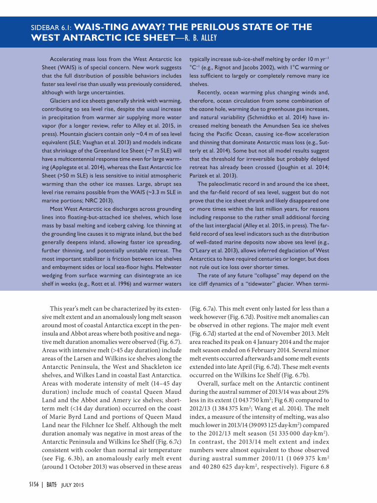
nating on land, glaciers typically taper to a thin edge. When terminating in water, for example, a tidewater glacier, the glacier front is a cliff. This is a result of an inherent instability caused by any preferential retreat of the above-waterline or below-waterline section of the glacier cliff face. With preferential retreat of the subaerial portion, the force of floatation on the subaqueous cliff causes a new fracture to form, returning the glacier front to a vertical; the same is true if the subaqueous section temporarily retreats faster. (Preferential melting at the water line increases the imbalance both above and below.) Subaerial ice cliffs (see Fig. SB6.1 for an example) can be stable up to a maximum height that likely is ~100 m (e.g., Hanson and Hooke 2003; Bassis and Walker 2012), near the greatest cliff height now observed. Retreat of shorter cliffs following ice-shelf loss is delayed, limiting the rate of sea level rise, because further iceberg calving does not occur until normal “viscous” flow processes reduce the ice-front thickness close to flotation (Joughin et al. 2008).

If current climate and cryosphere trends continue in the WAIS sector, and a strong stabilizing ice shelf does not reform, sufficient retreat along Thwaites Glacier in the Amundsen Sea drainage should produce an ice cliff much higher than the estimated ~100 m maximum. If melting or drift can rapidly remove ice supplied to the ocean, brittle cliff failure without prior thinning to flotation might cause rapid ice-sheet shrinkage. Adding a parameterization for this process to a comprehensive ice-sheet model shifted

ice sheet loss to a subcentury time scale after sufficient warmth and retreat were achieved (Pollard et al. 2015).

These considerations do not mean that “catastrophic” retreat (meters of sea level rise in decades) is inevitable, nor do they imply that any catastrophic retreat must start soon. They do however highlight important improvements needed in modeling and observations, and demonstrate that accurate worst-case scenarios for sea level rise are likely to exhibit shorter time scales than indicated by much prior work.

Fig. SB6.1. The front of Jakobshavn Isbrae, Greenland. The glacier front is near flotation, so the ~100 m high subaerial cliff overlies a much deeper submarine cliff. The sets of en echelon cracks (some shown by purple arrows) indicate incipient cliff failure. Photo by the author.

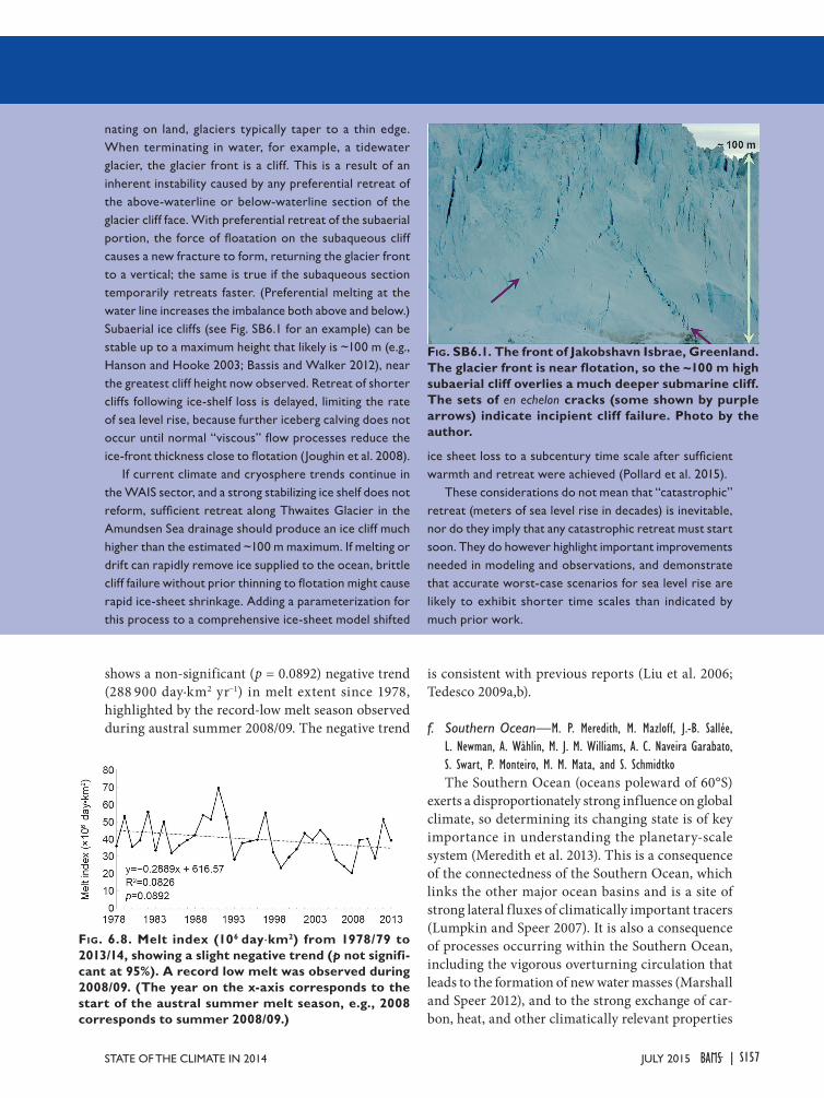
Fig. 6.8. Melt index (106 day·km2) from 1978/79 to 2013/14, showing a slight negative trend (p not signifi-cant at 95%). A record low melt was observed during 2008/09. (The year on the x-axis corresponds to the start of the austral summer melt season, e.g., 2008 corresponds to summer 2008/09.)

shows a non-significant (p = 0.0892) negative trend (288 900 day·km2 yr−1) in melt extent since 1978, highlighted by the record-low melt season observed during austral summer 2008/09. The negative trend

is consistent with previous reports (Liu et al. 2006; Tedesco 2009a,b).

f. Southern Ocean—M. P. Meredith, M. Mazloff, J.-B. Sallée, L. Newman, A. Wåhlin, M. J. M. Williams, A. C. Naveira Garabato, S. Swart, P. Monteiro, M. M. Mata, and S. SchmidtkoThe Southern Ocean (oceans poleward of 60°S)

exerts a disproportionately strong influence on global climate, so determining its changing state is of key importance in understanding the planetary-scale system (Meredith et al. 2013). This is a consequence of the connectedness of the Southern Ocean, which links the other major ocean basins and is a site of strong lateral fluxes of climatically important tracers (Lumpkin and Speer 2007). It is also a consequence of processes occurring within the Southern Ocean, including the vigorous overturning circulation that leads to the formation of new water masses (Marshall and Speer 2012), and to the strong exchange of car-bon, heat, and other climatically relevant properties


at the ocean surface (Sallée et al. 2012). However, de-termining the state of the Southern Ocean in a given year is even more problematic than for other ocean basins, due to the paucity of observations (see Sidebar 6.2). Nonetheless, using the limited data available, some key aspects of the state of the Southern Ocean in 2014 can be ascertained.

1) Surface temperature and circulation Sea surface temperature (SST) is examined here for

the interval June 2002 –December 2014. Temporal SST variability is dominated by the seasonal cycle, which explains ~30% of the variance in the Antarctic Cir-cumpolar Current (ACC) and >60% in its flanks, but which is far less significant in the polar gyres (regions of cyclonic oceanic circulation). After removal of the seasonal cycle, the mean (de-seasonalized) 2014 SST is compared with the long-term mean (Fig. 6.9a). The most noticeable signals are higher-than-average SST in the South Pacific Ocean, but lower-than-average SST just east and west of Drake Passage during 2014, consistent with the annual mean low-pressure anomaly in the Amundsen Sea (Fig. 6.6c).

Surface circulation is assessed here using satellite altimeter-derived sea surface height (SSH) measure-ments for the period 1993–2014. The mean 2014 SSH is compared to the long-term mean for the previous years (Fig. 6.9b), after removal of a linear trend. This ~3 mm yr−1 trend (Fig. 6.9c,d) is the dominant SSH signal, explaining ~10% of the variance over much of the region and >50% in the southwest Pacific Ocean. In 2014, the residual SSH was generally higher than previous years, thereby suggesting an acceleration of the trend. The anomalously high SST and SSH in the South Pacific Ocean in 2014 suggest steric heating is partly responsible. This is not the case for the polar gyres. Stronger SSH anomalies north of the ACC compared to the south lead to increased sea level slope across the ACC, suggesting stronger-than-usual circumpolar flow in 2014. By contrast, the southwest Indian Ocean shows an opposite anomaly in slope, suggesting a weaker Agulhas retroflection.

2) upper-ocean Stratification

Changes in the mixed-layer depth (MLD) have significant implications for both physical and bioge-ochemical processes occurring in the ocean and the overlying atmosphere. Intermediate waters subducted in the Southern Ocean ventilate the thermocline of the Southern Hemisphere subtropical gyres and con-tribute to global budgets of heat, fresh water, nutri-ents, and carbon, while anomalies in MLD modulate the exchange of oxygen, heat, and carbon between

Fig. 6.9. (a) 2014 mean SST minus the Jun 2002–Dec 2013 mean SST (°C). The annual cycle has been re-moved prior to averaging. (Source: Microwave SST data produced by Remote Sensing Systems, www .remss.com.) (b) 2014 mean SSH minus the 1993–2013 mean (cm). The linear trend has been removed prior to averaging. (Source: Ssalto/Duacs.) (c) The 1993–2014 linear SSH trend (mm yr–1). (d) The percent variance explained by the linear SSH trend. (e) 2000–13 clima-tological winter (Sep) MLD (m) (following Sallée et al. 2006) in the Southern Ocean; (f) Scatter plot of the MLD anomaly (anomaly from the local climatological seasonal cycle) for all Argo float observations sampled between 1 Jan and 1 Dec 2014. The black lines show, from south to north, the mean position of the Polar, Subantarctic, and the northern branch of the Subant-arctic Fronts.The sea ice masking varies between pan-els/data sources, and is mainly a function of omitting missing data in each panel.

the ocean and the atmosphere (e.g., Lovenduski and Gruber 2005; Sarmiento et al. 2004).

The Argo Float Program now provides >10 years of temperature and salinity profiles, allowing the computation of robust climatologies of MLD for the

S158 JULY 2015|

SIDEBAR 6.2: THE SOUTHERN OCEAN OBSERVING SYSTEM (SOOS)—M. P. MEREDITH, M. MAZLOFF, J.-B. SALLÉE, L. NEWMAN, A. WÅHLIN, M. J. M. WILLIAMS, A. C. N. GARABATO, S. SWART, P. MONTEIRO, M. M. MATA, AND S. SCHMIDTKO

The Southern Ocean is integral to the operation of the Earth system, strongly inf luencing global climate and planetary-scale biogeo-chemical cycles through its central role in driving ocean circulation, global biologi-cal productivity, and up-take of atmospheric carbon (Fig. SB6.2). Yet the ability to understand the evolving state of the Southern Ocean and to detect changes with an ac-ceptable degree of certainty is severely limited by the paucity of observations. A number of sensor technolo-gies, such as Argo floats, sat-ellite remote sensing, and the tagging of marine mammals provide data in near-real time with wide-area coverage, and can be used to make some deductions on the current state of the Southern Ocean. However, these data streams are the exception, with most observations being collected through short-term, regionally-specific projects that have data delivery delays of months to years.

The Southern Ocean Observing System (SOOS; www .soos.aq) was developed from the community-driven need for sustained and integrated delivery of observational data that are fundamental to the understanding of dynamics and change in Southern Ocean systems. The SOOS mission is to facilitate, internationally, the collection and delivery of essential observations on dynamics and change of Southern Ocean systems to all stakeholders (researchers, governments, industries), through the design, promotion, and implementation of cost-effective observation and data delivery systems.

SOOS has identified four key goals necessary for achieving its mission:

1) A coordinated, integrated, efficient, and sustained in-ternational program to deliver time series of observa-tions of essential elements of Southern Ocean systems;

2) Regional implementation of the observing systems to achieve circumpolar coverage of the Southern Ocean;

3) Facilitation and promotion of activities to improve observing Southern Ocean systems, through inter-

national coordination and technological research and development, including the affiliation of projects and programs with this work;

4) Efficient and internationally integrated data man-agement systems to enable stakeholders to access observations and synthesis products on the dynamics and change of Southern Ocean systems.

Even if the current level of investment by the nations involved in Southern Ocean research is maintained, the logistical demands and costs associated with traditional methods of collecting observations (e.g., from research vessels) will likely prohibit collection at the spatial and temporal resolutions required. The long-term solution is progressively greater automation of data collection, with much greater use of technologies that can be operated remotely or completely autonomously. Aligned with a data management system that delivers the data in real time and a cyberinfrastructure system that enables the implementation of an effective adaptive sampling strat-egy, SOOS will deliver the observations and products required to determine the state of the Southern Ocean on an ongoing basis, in order to detect, attribute, and mitigate change.

SOOS is an initiative of the Scientific Committee on Oceanic Research (SCOR) and the Scientific Committee on Antarctic Research (SCAR).

Fig. SB6.2. Schematic of the scientific and societal drivers that require sustained observation of the Southern Ocean. From Meredith et al. (2013).


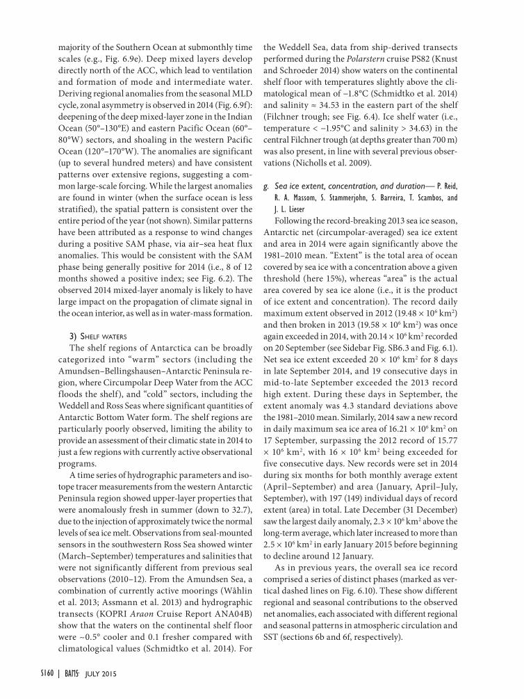
majority of the Southern Ocean at submonthly time scales (e.g., Fig. 6.9e). Deep mixed layers develop directly north of the ACC, which lead to ventilation and formation of mode and intermediate water. Deriving regional anomalies from the seasonal MLD cycle, zonal asymmetry is observed in 2014 (Fig. 6.9f): deepening of the deep mixed-layer zone in the Indian Ocean (50°–130°E) and eastern Pacific Ocean (60°–80°W) sectors, and shoaling in the western Pacific Ocean (120°–170°W). The anomalies are significant (up to several hundred meters) and have consistent patterns over extensive regions, suggesting a com-mon large-scale forcing. While the largest anomalies are found in winter (when the surface ocean is less stratified), the spatial pattern is consistent over the entire period of the year (not shown). Similar patterns have been attributed as a response to wind changes during a positive SAM phase, via air–sea heat flux anomalies. This would be consistent with the SAM phase being generally positive for 2014 (i.e., 8 of 12 months showed a positive index; see Fig. 6.2). The observed 2014 mixed-layer anomaly is likely to have large impact on the propagation of climate signal in the ocean interior, as well as in water-mass formation.

3) Shelf waterS

The shelf regions of Antarctica can be broadly categorized into “warm” sectors (including the Amundsen–Bellingshausen–Antarctic Peninsula re-gion, where Circumpolar Deep Water from the ACC floods the shelf), and “cold” sectors, including the Weddell and Ross Seas where significant quantities of Antarctic Bottom Water form. The shelf regions are particularly poorly observed, limiting the ability to provide an assessment of their climatic state in 2014 to just a few regions with currently active observational programs.

A time series of hydrographic parameters and iso-tope tracer measurements from the western Antarctic Peninsula region showed upper-layer properties that were anomalously fresh in summer (down to 32.7), due to the injection of approximately twice the normal levels of sea ice melt. Observations from seal-mounted sensors in the southwestern Ross Sea showed winter (March–September) temperatures and salinities that were not significantly different from previous seal observations (2010–12). From the Amundsen Sea, a combination of currently active moorings (Wåhlin et al. 2013; Assmann et al. 2013) and hydrographic transects (KOPRI Araon Cruise Report ANA04B) show that the waters on the continental shelf f loor were ~0.5° cooler and 0.1 fresher compared with climatological values (Schmidtko et al. 2014). For

the Weddell Sea, data from ship-derived transects performed during the Polarstern cruise PS82 (Knust and Schroeder 2014) show waters on the continental shelf floor with temperatures slightly above the cli-matological mean of −1.8°C (Schmidtko et al. 2014) and salinity ≈ 34.53 in the eastern part of the shelf (Filchner trough; see Fig. 6.4). Ice shelf water (i.e., temperature < −1.95°C and salinity > 34.63) in the central Filchner trough (at depths greater than 700 m) was also present, in line with several previous obser-vations (Nicholls et al. 2009).

g. Sea ice extent, concentration, and duration— P. Reid, R. A. Massom, S. Stammerjohn, S. Barreira, T. Scambos, and J. L. LieserFollowing the record-breaking 2013 sea ice season,

Antarctic net (circumpolar-averaged) sea ice extent and area in 2014 were again significantly above the 1981–2010 mean. “Extent” is the total area of ocean covered by sea ice with a concentration above a given threshold (here 15%), whereas “area” is the actual area covered by sea ice alone (i.e., it is the product of ice extent and concentration). The record daily maximum extent observed in 2012 (19.48 × 106 km2) and then broken in 2013 (19.58 × 106 km2) was once again exceeded in 2014, with 20.14 × 106 km2 recorded on 20 September (see Sidebar Fig. SB6.3 and Fig. 6.1). Net sea ice extent exceeded 20 × 106 km2 for 8 days in late September 2014, and 19 consecutive days in mid-to-late September exceeded the 2013 record high extent. During these days in September, the extent anomaly was 4.3 standard deviations above the 1981–2010 mean. Similarly, 2014 saw a new record in daily maximum sea ice area of 16.21 × 106 km2 on 17 September, surpassing the 2012 record of 15.77 × 106 km2, with 16 × 106 km2 being exceeded for five consecutive days. New records were set in 2014 during six months for both monthly average extent (April–September) and area (January, April–July, September), with 197 (149) individual days of record extent (area) in total. Late December (31 December) saw the largest daily anomaly, 2.3 × 106 km2 above the long-term average, which later increased to more than 2.5 × 106 km2 in early January 2015 before beginning to decline around 12 January.

As in previous years, the overall sea ice record comprised a series of distinct phases (marked as ver-tical dashed lines on Fig. 6.10). These show different regional and seasonal contributions to the observed net anomalies, each associated with different regional and seasonal patterns in atmospheric circulation and SST (sections 6b and 6f, respectively).

S160 JULY 2015|

1) January–mid-april

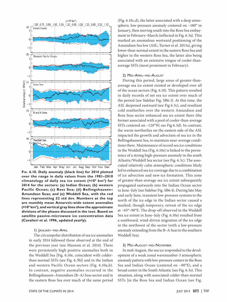
The circumpolar distribution of sea ice anomalies in early 2014 followed those observed at the end of the previous year (see Massom et al. 2014). There were persistently high positive anomalies both in the Weddell Sea [Fig. 6.10e, coincident with colder-than-normal SSTs (see Fig. 6.3b)] and in the Indian and western Pacific Ocean sectors (Fig. 6.10a,b). In contrast, negative anomalies occurred in the Bellingshausen–Amundsen (B–A) Seas sector and in the eastern Ross Sea over much of the same period

Fig. 6.10. Daily anomaly (black line) for 2014 plotted over the range in daily values from the 1981–2010 climatology of daily sea ice extent (×106 km2) for 2014 for the sectors: (a) Indian Ocean; (b) western Pacif ic Ocean; (c) Ross Sea; (d) Bellingshausen–Amundsen Seas; and (e) Weddell Sea, with the red lines representing ±2 std dev. Numbers at the top are monthly mean Antarctic-wide extent anomalies (×106 km2), and vertical gray lines show the approximate divisions of the phases discussed in the text. Based on satellite passive-microwave ice concentration data (Cavalieri et al. 1996, updated yearly).

(Fig. 6.10c,d), the latter associated with a deep atmo-spheric low-pressure anomaly centered on ~180° in January, then moving south into the Ross Sea embay-ment in February–March (reflected in Fig. 6.3a). This marked an anomalous westward positioning of the Amundsen Sea low (ASL; Turner et al. 2013a), giving lower-than-normal extent in the eastern Ross Sea and higher in the western Ross Sea, the latter also being associated with an extensive tongue of cooler-than-average SSTs (most prominent in February).

2) mid-april–mid-auguSt

During this period, large areas of greater-than-average sea ice extent existed or developed over all of the ocean sectors (Fig. 6.10). This pattern resulted in daily records of net sea ice extent over much of the period (see Sidebar Fig. SB6.3). At this time, the ASL deepened eastward (see Fig 6.3c), and resultant cold southerlies over the western Amundsen and Ross Seas sector enhanced sea ice extent there (the former associated with a pool of cooler-than-average SSTs centered on ~120°W; see Fig 6.3d). In contrast, the warm northerlies on the eastern side of the ASL impacted the growth and advection of sea ice in the Bellingshausen Sea, to maintain near-average condi-tions there. Maintenance of record sea ice conditions in the Weddell Sea (Fig. 6.10e) is linked to the persis-tence of a strong high-pressure anomaly in the south Atlantic/Weddell Sea sector (see Fig. 6.3c). The asso-ciated relatively calm atmospheric conditions likely led to enhanced sea ice coverage due to a combination of ice advection and new-ice formation. This zone of greater-than-average sea ice extent subsequently propagated eastwards into the Indian Ocean sector in June–July (see Sidebar Fig. SB6.4). During late May and early June, transient low-pressure systems to the north of the ice edge in the Indian sector caused a marked, though temporary, retreat of the ice edge at ~65°–90°E. The drop-off observed in the Weddell Sea ice extent in June–July (Fig. 6.10e) resulted from a southward, wind-driven migration of the ice edge in the northwest of the sector (with a low-pressure anomaly extending from the B–A Seas to the southern Weddell Sea).

3) mid-auguSt–mid-november In mid-August, the sea ice responded to the devel-

opment of a weak zonal wavenumber-3 atmospheric anomaly pattern with low-pressure centers in the Ross Sea and Indian Ocean (centered on ~90°E), and a broad center in the South Atlantic (see Fig. 6.3e). This situation, along with associated colder-than-normal SSTs [in the Ross Sea and Indian Ocean (see Fig.


6.3f)], led to ice expansion in the Ross, western Wed-dell, and Indian Ocean sectors, while a suppression of ice advance occurred in the B–A Seas sector. The

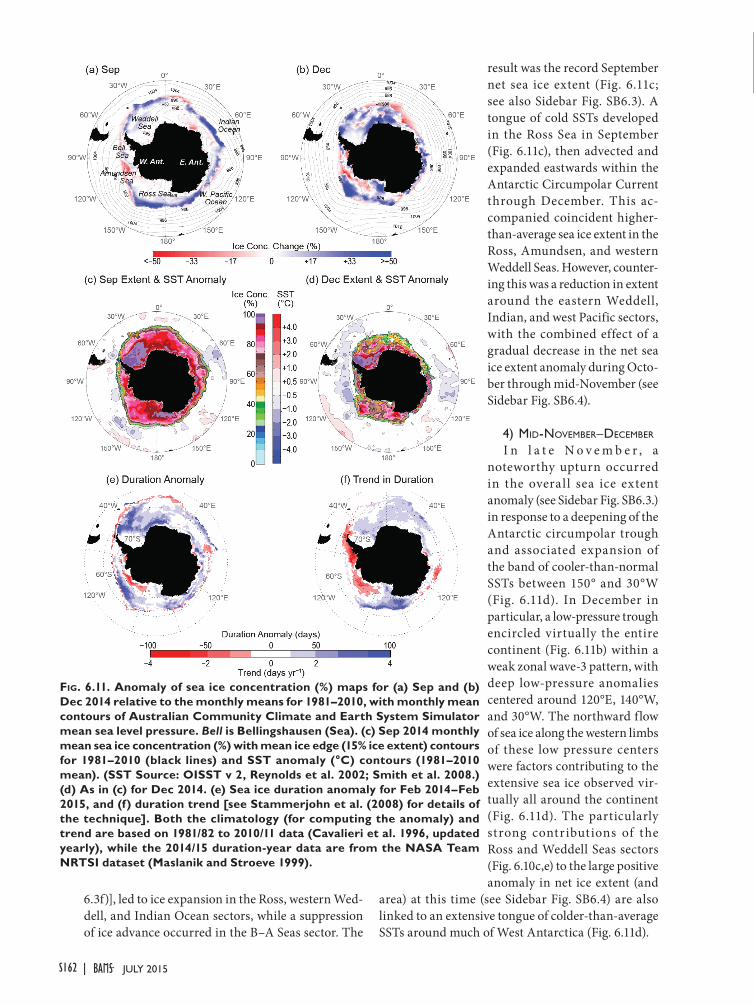
Fig. 6.11. Anomaly of sea ice concentration (%) maps for (a) Sep and (b) Dec 2014 relative to the monthly means for 1981–2010, with monthly mean contours of Australian Community Climate and Earth System Simulator mean sea level pressure. Bell is Bellingshausen (Sea). (c) Sep 2014 monthly mean sea ice concentration (%) with mean ice edge (15% ice extent) contours for 1981–2010 (black lines) and SST anomaly (°C) contours (1981–2010 mean). (SST Source: OISST v 2, Reynolds et al. 2002; Smith et al. 2008.) (d) As in (c) for Dec 2014. (e) Sea ice duration anomaly for Feb 2014–Feb 2015, and (f) duration trend [see Stammerjohn et al. (2008) for details of the technique]. Both the climatology (for computing the anomaly) and trend are based on 1981/82 to 2010/11 data (Cavalieri et al. 1996, updated yearly), while the 2014/15 duration-year data are from the NASA Team NRTSI dataset (Maslanik and Stroeve 1999).

result was the record September net sea ice extent (Fig. 6.11c; see also Sidebar Fig. SB6.3). A tongue of cold SSTs developed in the Ross Sea in September (Fig. 6.11c), then advected and expanded eastwards within the Antarctic Circumpolar Current through December. This ac-companied coincident higher-than-average sea ice extent in the Ross, Amundsen, and western Weddell Seas. However, counter-ing this was a reduction in extent around the eastern Weddell, Indian, and west Pacific sectors, with the combined effect of a gradual decrease in the net sea ice extent anomaly during Octo-ber through mid-November (see Sidebar Fig. SB6.4).

4) mid-november–december

I n l a t e N o v e m b e r , a noteworthy upturn occurred in the overall sea ice extent anomaly (see Sidebar Fig. SB6.3.) in response to a deepening of the Antarctic circumpolar trough and associated expansion of the band of cooler-than-normal SSTs between 150° and 30°W (Fig. 6.11d). In December in particular, a low-pressure trough encircled virtually the entire continent (Fig. 6.11b) within a weak zonal wave-3 pattern, with deep low-pressure anomalies centered around 120°E, 140°W, and 30°W. The northward flow of sea ice along the western limbs of these low pressure centers were factors contributing to the extensive sea ice observed vir-tually all around the continent (Fig. 6.11d). The particularly strong contributions of the Ross and Weddell Seas sectors (Fig. 6.10c,e) to the large positive anomaly in net ice extent (and

area) at this time (see Sidebar Fig. SB6.4) are also linked to an extensive tongue of colder-than-average SSTs around much of West Antarctica (Fig. 6.11d).

S162 JULY 2015|

SIDEBAR 6.3: SUCCESSIVE ANTARCTIC SEA ICE EXTENT RECORDS DURING 2012, 2013, AND 2014—P. REID AND R. A. MASSOM

The calendar years of 2012, 2013, and 2014 saw succes-sive records in annual daily maximum (ADM) net Antarctic sea ice extent based on satellite data since 1979 (Massom et al. 2013, 2014; section 6g), continuing the trend over the past three decades of an overall increase in Antarctic sea ice extent (Comiso 2010; Parkinson and Cavalieri 2012) and contributing to regional changes in sea ice seasonality (Stammerjohn et al. 2012). However, the mechanisms and associated regional anomalies involved in achieving each of these records were quite different.

In 2012, sea ice extent tracked close to or slightly above average for much of the year (Fig. SB6.3); however, the development of an atmospheric wave-3 pattern dur-ing August and September caused rapid expansion of the ice edge during that period (Fig. SB6.4), particularly in the western Pacific Ocean sector (Turner et al. 2013b; Massom et al. 2013), and a new ADM was recorded in late September. The year 2013 saw quite different factors involved in achieving the record extent, with a tongue of colder-than-normal SSTs in the western Ross Sea sector aiding the early advance of sea ice in that region (Fig. SB6.4 and Massom et al. 2013; Reid et al. 2015). This SST anomaly subsequently advected eastwards after reaching the Antarctic Circumpolar Current in about June 2013, to envelop the ice edge to the north of the Bellingshausen–Amundsen Seas region and aid further thermo-dynamic expansion of ice there as the year progressed (Fig. SB6.3). Net ice extent was well above average all of 2013 (Fig. SB6.3), with many daily records set be-fore the ADM was once again broken in late September. In 2014, greater-than-average sea ice extent in the Weddell Sea was the predominant contribu-tor to the well-above-average net Antarctic sea ice extent early in the year (Figs. SB6.3, SB6.4), with colder-than-normal SSTs to the north of the ice edge in the Weddell Sea (see Fig. 6.3b) influ-encing a late 2013/14 retreat and subsequent early annual advance in that region. As the 2014 season progressed, the area of above-average sea ice extent expanded

farther to the east, leading to anomalously expansive sea ice coverage over much of the Indian Ocean sector for the rest of the year (Fig. SB6.4). This was augmented by midseason wind-driven ice advance in the western Pacific Ocean and Ross Sea to create a new ADM on 20 September 2014 (see Fig. 6.1).

Fig. SB6.3. 5-day running mean of 2012 (green), 2013 (light blue), and 2014 (dark blue) daily sea ice extent anomaly relative to the 1981–2010 mean (×106 km2) for the Southern Hemisphere. The shaded banding represents the range of daily values for 1981–2010.

Fig. SB6.4. Anomalies of daily sea ice extent [× 103 km2 (degree longitude)–1] from Jan 2012 to Dec 2014 represented as a Hovmöller. The values represent the areal extent of the anomaly integrated over a 1° longitude to the north of the continental edge (× 103 km2). Note that the longitudes are repeated to display the spatial continuity of the sea ice extent anomalies.


Consistent with the mostly positive sea ice extent anomalies described for the first half of the year (Fig. 6.10), the timing of the fall/early winter ice-edge advance was earlier than normal (by 10–70 days) in all sectors except: (1) the southern BAS sector; and (2) the Ross Sea sector between 160°E and 160°W, where the ice-edge advance was instead later than normal (by 10 to ~30 days). There was some correspondence between the 2013/14 ice retreat anomaly pattern (Massom et al. 2014) and the 2014 ice advance pattern, particularly for: 1) the western Weddell and Indian Ocean sectors (where the 2013/14 spring retreat was anomalously late, followed by an anomalously early 2014 fall advance); and 2) the outer pack ice of the Bellingshausen Sea (where the 2013/14 spring retreat was anomalously early, followed by an anomalously late 2014 fall advance). Most notable, however, were the strong earlier-than-normal anomalies in the ice edge advance throughout the Weddell Sea sector between 0° and 60°W and the East Antarctic sector between 90°E and 160°E. In contrast, there was a remarkable recovery and acceleration of the ice-edge advance in the outer pack ice of the BAS and

eastern Ross Sea sectors (between 80°W to 160°W) later in the 2014 fall season. This area showed a sharp switch from late to early ice-edge advance anomalies south-to-north. This recovery and acceleration of the ice-edge advance corresponded to the eastward movement of the ASL (described above; see Fig. 6.3c) and strengthening of cold southerly winds in the eastern Ross Sea sector in May–June. Subsequently, a broad band of cold SSTs developed along the advancing ice edge between 90°W and 160°W (see Fig. 6.3d), which may explain the recovery and rapid advance of the ice edge.

The anomaly pattern for the 2014/15 spring–summer sea ice retreat was considerably less striking than the ice advance anomaly pattern just described, showing in general smaller anomalies. There were, however, some interesting contrasts: the outer Weddell Sea and most of the East Antarctic sector showed an earlier retreat (in contrast to the earlier advance previously experienced there), while the Ross Sea sector between 160°E and 160°W showed a later retreat (in contrast to the later advance previously experienced there). Nonetheless, the ice season

Analyses of trends in sea ice extent and seasonality (see Fig. 6.11g) over the last few decades show that the overall increase in Antarctic coverage comprises contrast-ing regional contributions: strong increases in ice extent and duration in the Ross Sea and moderate increases elsewhere except for strong decreases in the western Antarctic Peninsula–Bellingshausen Sea region (WAP–BS). These trends are attributed predominantly to changes in wind patterns (Holland and Kwok 2012; Parkinson and Cavalieri 2012; Stammerjohn et al. 2012), although some research suggests an association with changes in fresh-water fluxes (Liu and Curry 2010; Bintanja et al. 2013). The overall patterns of ice extent anomaly for the last three years (2012–14) are not fully consistent with these regional trends, except in the western Ross Sea where there have been persistent positive anomalies for the last three years (Fig. SB6.4). Ice extent in the WAP–BS was close to or above normal over this three-year period, and was particularly high in 2013 (Fig. SB6.4), in contrast to the long-term trend. The regional anomalies over these last three years are, however, consistent with associated patterns of large-scale drivers of sea ice formation, distri-bution, and retreat, that is, regional atmospheric synoptic patterns and ocean circulation and temperature.

Given that there were three record-breaking years in a row, it is well worth asking: Did the pattern of sea ice extent, and the associated retreat, in one year influence

the pattern of extent and ice advance in the following year? The answer: Quite probably. Several studies have suggested that the pattern of sea ice retreat in one year can influence the advance in the subsequent year (Nihashi and Ohshima 2001; Stammerjohn et al. 2012; Holland 2014), and this appears to be the case, particularly in these last three years. From September 2012 onwards, there is a clear eastward propagation of sea ice extent anomaly stemming from the western Pacific Ocean sector, through the Ross, Bellingshausen, and Amundsen Seas during 2013 and into the Weddell Sea in early 2014 (Fig. SB6.4). The positive ice anomaly in the western Pacific region in August–September 2012, as the result of the deep low pressure in that region, may have slowed the western coastal currents and subsequently caused the cold ocean surface temperatures and hence early advance of sea ice in the western Ross Sea in 2013. Similarly, the anomalous positive extent in sea ice in the WAP–BS sector in late 2013 may have impacted the late retreat and early ad-vance of sea ice in the Weddell Sea in 2013/14. Much of this is speculation, but there is no one specific underlying mechanism that can easily explain these three years of record-breaking sea ice extent. Indeed, Antarctic sea ice continues to behave and respond in a complex fashion by integrating influences from the atmosphere, ocean, and wider cryosphere.

CONT. SIDEBAR 6.3: SUCCESSIVE ANTARCTIC SEA ICE EXTENT RECORDS DURING 2012, 2013, AND 2014—P. REID AND R. A. MASSOM

S164 JULY 2015|

duration anomalies (Fig. 6.11f) were mostly positive in those two sectors (indicating a longer-than-normal ice season), due to the early advance anomalies being larger than the early retreat anomalies. The eastern Ross and western Amundsen Sea sectors (between 130° and 150°W) showed both an earlier advance and later retreat, contributing to a much longer-than-normal ice season duration (Fig. 6.11f). Thus, in general, most of the ice season duration anomalies are positive and are consistent with long-term trends in ice season duration (Fig. 6.11g; Stammerjohn et al. 2012; Holland 2014), with the notable exception of the B–A Seas sector, which experienced near-normal ice season duration in contrast to the strong trend there towards shorter ice seasons.

h. Ozone depletion—P. A. Newman, E. R. Nash , S. E. Strahan, N. Kramarova, C. S. Long, M. C. Pitts, B. Johnson, M. L. Santee, I. Petropavlovskikh, and G. O. BraathenThe Antarctic ozone hole is showing weak evi-

dence of a decrease in area, based upon the last 15 years of ground and satellite observations. The 2014 Antarctic stratospheric ozone depletion was less se-vere compared to the 1995–2005 average, but ozone levels were still low compared to pre-1990 levels. Figure 6.12a displays the average column ozone between 12 and 20 km derived from NOAA South Pole balloon profiles. The 2014 South Pole ozone column inventory was relatively high with respect to a 1991–2006 average (horizontal line), and in fact, all of the 2009–2014 ozone column inventories were higher than the 1991–2006 average. The 1998–2014 period shows a positive secular trend (blue line), excluding 2002 (the year with a major stratospheric sudden warming; Roscoe et al. 2005).

Satellite column observations over Antarctica (poleward of 60°S) also show a steady ozone increase since the late-1990s. Figure 6.12b shows the average of daily minimum total column ozone values over the 21 September to 16 October period (ozone hole peak period). This average of daily values is increas-ing at a rate of 1.4 DU yr−1 (90% confidence level). Excluding the anomalous 2002 value, the trend be-comes 1.9 DU yr−1 (99% confidence level).

The 2014 ozone hole area was 20.9 million km2 (averaged from the 7 September–13 October daily es-timates), the sixth smallest over the 1991–2014 period. The area trend since 1998 shows that the ozone hole is decreasing at a rate of 0.17 million km2 yr−1, but this trend is not statistically significant. As with Fig. 6.12b, if the 2002 sudden warming outlier is excluded, the trend becomes significant at −0.29 million km2 yr−1 (p < 0.05).

Attribution of ozone hole shrinkage is still dif-ficult. Antarctic stratospheric ozone depleting substances are estimated using equivalent effective stratospheric chlorine (EESC)—a combination of inorganic chlorine and bromine. A mean age of 5.2 years is used to estimate EESC (Strahan et al. 2014). Since the 2000–02 peak of 3.79 ppb, EESC has de-creased to 3.45 ppb (a decrease of 0.34 ppb or 9%). This is a 20% drop towards the 1980 level of 2.05 ppb, where 1980 is considered to be a “pre-ozone hole” pe-riod. Aura satellite Microwave Limb Sounder (MLS)

Fig. 6.12. (a) Column ozone (DU) measured within the 12–20 km primary depletion layer by NOAA South Pole ozonesondes during 21 Sep–16 Oct over 1986–2014. The blue line shows the 1998–2014 trend. (b) Satellite daily total ozone minimum values (DU) averaged over 21 Sep–16 Oct. (c) 50-hPa Sep tem-peratures (K) in the 60°–90°S region for MERRA (black points) and for NCEP/NCAR reanalyses (red points, bias adjusted to mean MERRA values). The horizontal line indicates the 1991–2006 for (a) and (b), and the 1979–2014 average for (c).


The ozone hole typically breaks-up in the mid-November to mid-December period; the 2014 ozone hole broke up around 4 December (the approximate average break-up date for the last 20 years). This “break-up” is estimated to be when total ozone val-ues < 220 DU disappear from the Antarctic region. The ozone break-up is tightly correlated with the lower stratospheric polar vortex break-up. The vor-tex break-up is driven by wave events propagating upward into the stratosphere. These wave events also mix ozone-rich midlatitude air into the polar region in the 550–750 K layer. While 2012 and 2013 ozone

N2O measurements can also be used to estimate Antarctic stratospheric inorganic chlorine (Cly) levels (Strahan et al. 2014) and to quantify their transport-driven interannual variability. The 2014 Antarctic stratospheric Cly was higher than in recent years and similar to levels found in 2008 and 2010.

Satellite observations of chlorine and ozone in the 2014 Antarctic lower stratosphere were not ex-ceptionally different from those in the last 10 years. Observations of hydrogen chloride (HCl; Fig. 6.13a), chlorine monoxide (ClO; Fig. 6.13b), and ozone (O3; Fig. 6.13c) are shown for the Antarctic polar vortex. The reaction of HCl with ClONO2 (chlorine nitrate) on the surfaces of polar stratospheric cloud (PSC) particles forms chlorine gas (Cl2) and causes HCl to decline during the June–July period (Fig. 6.13a). Cl2 is easily photolyzed by visible light, and the ozone reactive ClO steadily increases as the sun returns to Antarctica (Fig. 6.13b). Chlorine and ozone in the Antarctic stratosphere in 2014 (Fig. 6.13b,c, blue lines) were within the 2004–13 climatology (gray shading).

Another key factor for the Antarctic ozone hole severity is stratospheric temperature. Colder tem-peratures lead to more severe depletion and lower ozone levels. Figure 6.12c shows September Antarctic stratospheric temperatures (50 hPa, 60°–90°S) from NCEP (red) and MERRA (black) reanalyses. The 2014 temperatures were near the 1979–2014 mean, as reflected also by ERA-Interim in Fig. 6.2b.

The 2014 stratospheric dynamical conditions were also near-average. The 100-hPa eddy heat flux is a metric of both wave propagation into the strato-sphere and the strength of the downward motion over Antarctica. For example, in September 2002 the mag-nitude of the 100-hPa eddy heat flux was extremely high, the polar vortex underwent a stratospheric sudden warming, and the stratosphere was very warm (Fig. 6.12c). In contrast, the 2014 eddy heat flux was near-average for the August–September period and consequently, the stratospheric polar vortex and jet flow around Antarctica were near-average.

PSCs provide particle surfaces that enable hetero-geneous chemical reactions to release chlorine for catalytic ozone loss. Temperatures provide a useful proxy for PSCs, but the Cloud-Aerosol Lidar and Infrared Pathfinder Satellite Observation (CALIPSO) provides direct observations. Figure 6.13d displays the 2014 PSC volume (blue line). For the entire sea-son, the PSC volume generally followed the average (white line). The year 2006 had the highest volume at 65 million km3 averaged from June–October, while 2014 was near-average at 42 million km3 during the same months.

Fig. 6.13. Time series of 2014 Antarctic vortex-av-eraged (blue): (a) HCl in ppbv, (b) ClO in ppbv, and (c) ozone in ppmv from Aura MLS. The averages are made inside the polar vortex on the 485-K potential temperature surface (~21 km or 40 hPa). Gray shading shows 2004–13. (Updated from Manney et al. 2011.) (d) Time series (blue line) of CALIPSO PSC volume (×106 km3, updated from Pitts et al. 2009). The gray shading shows the 2006–13 range of values for each day and the white line is the average.

S166 JULY 2015|

holes broke-up earlier than usual due to stronger wave activity that enabled ozone-rich air transport from midlatitudes, the 2014 break-up of the ozone hole occurred close to the average date.

In summary, the Antarctic ozone hole is a severe ozone depletion that regularly appears in austral spring. In the last 14 years, the ozone hole has be-gun to display marginal signs of improvement (i.e., decrease in size). This improvement is statistically significant in observations from both ground and

satellite data, if the year 2002 is treated as an outlier (because of the major stratospheric sudden warming that occurred). Levels of chlorine continue to decline in the stratosphere because of the Montreal Protocol (WMO 2014), and this decline should be manifest in the Antarctic ozone hole. However, unambiguous attribution of the ozone hole improvement to the Montreal Protocol cannot yet be made because of relatively large year-to-year variability and observa-tional uncertainty.


ACKNOWLEDGMENTS

The report's editors wish to thank the AMS Journals editorial staff, in particular Melissa Fernau, for facilitating the document, and to the NCEI graphics team for laying the document out and executing the countless number of technical edits needed. We also wish to express our sincere and deep gratitude to Dr. Rick Rosen, who served as the AMS special editor for this report. Dr. Rosen's handling of the reviews was at the same time rigorous and responsive, and greatly improved the document.

Chapter 2:• The editors thank David Parker for his excellent internal review.• Kate Willett, Robert Dunn, David Parker, Chris Folland, Rob

Allan, and Colin Morice were supported by the Joint UK DECC/Defra Met Office Hadley Centre Climate Programme (GA01101).

• The datasets used for the Total Column Water Vapor and Cloudiness sections [sections 2d(2) and 2d(5)] were provided from the Japanese 55-year Reanalysis (JRA-55) project carried out by the Japan Meteorological Agency (JMA).

• The editors thank Paul Berrisford (European Centre for Medium-Range Weather Forecasts), Mike Bosilovich (NASA), Shinya Kobayashi (Japan Meteorological Agency) and Cathy Smith (NOAA) for timely provision of reanalysis data.

• Additional data were provided by: Environmental Model-ing Center/National Centers for Environmental Prediction/National Weather Service/NOAA/U.S. Department of Com-merce. NCEP Climate Forecast System Reanalysis (CFSR) Monthly Products, January 1979 to December 2010. Research Data Archive at the National Center for Atmospheric Research, Computational and Information Systems Laboratory. http://rda .ucar.edu/datasets/ds093.2/.

Chapter 3:• Acknowledgments: Sandra Bigley (NOAA/Pacific Marine

Environmental Laboratory) provided able editorial assistance.• Simone Alin, Scott Cross, and Dan Siedov provided useful

comments on an early draft of the chapter.• Gregory C. Johnson and John Lyman were supported by NOAA

Research and the NOAA Climate Program Office.• Simon Good was supported by the Joint UK DECC/Defra Met

Office Hadley Centre Climate Programme (GA01101).• Catia M. Domingues was supported by an Australian Research

Council Future Fellowship (FT130101532).• Jeff Dunn provided quality-controlled Argo data (2000–2013)

and Neil White processed altimeter data for the CSIRO/ACE CRCIMAS-UTAS OHCA estimates.

Chapter 4:• Acknowledgements: Mark Lander (University of Guam) and

Charles ‘”Chip” Guard (National Weather Service, Guam Weather Forecast Office) for providing valuable inputs related to the section on Western North Pacific tropical cyclones.

• Bill Ward (NOAA/NWS Pacific Region Headquarters) who was involved with the internal review of the chapter.

Chapter 5:• For support for co-editing the Arctic section, Martin Jeffries

thanks the Office of Naval Research, and Jackie Richter-Menge thanks the NOAA Arctic Research Office. They also thank the authors for their contributions, and the reviewers for their thoughtful and constructive comments.

• Jim Overland’s contribution to the Air Temperature essay was supported by the NOAA Arctic Research Project of the Climate Program Office and by the Office of Naval Research, Code 322.

• Germar Bernhard and co-authors of the Ozone and UV Radia-tion essay acknowledge the support of the U.S. National Sci-ence Foundation (grant ARC-1203250), a Research Council of Norway Centres of Excellence award (project number 223268/F50) to the Norwegian Radiation Protection Authority, and the Academy of Finland for UV measurements by the FARPOCC and SAARA projects in Finland.

• Vladimir Romanovsky and co-authors of the Permafrost essay acknowledge the support of the State of Alaska, the National Science Foundation (grants PLR-0856864 and PLR-1304271 to the University of Alaska Fairbanks; PLR-1002119 and PLR-1304555 to the George Washington University), and by Geologi-cal Survey of Canada and Natural Resources Canada. Support was also provided by the Russian Science Foundation (projects 13-05-41509 RGO, 13-05-00811, 13-08-91001, 14-05-00956, 14-17-00037, and 15-55-71004) and by the government of the Russian Federation.

• Matthew Shupe’s contribution to Sidebar 5.1: Challenge of Arctic Clouds and their Implications for Surface Radiation was supported by the U.S. Department of Energy (DE-SC0011918) and National Science Foundation (PLR1314156).

• Howie Epstein, Gerald Frost and Skip Walker acknowledge the support of the NASA Land Cover Land Use Change Program for their contribution to Sidebar 5.2: Declassified High-Resolution Visible Imagery for Observing the Arctic.

Chapter 6:• Special thanks to Dr. Marilyn Raphael and Dr. Florence Fetterer

for their internal reviews of the chapter.• The work of Rob Massom, Phil Reid, and Jan Lieser was sup-

ported by the Australian Government’s Cooperative Research Centre program through the Antarctic Climate and Ecosystems CRC, and contributes to AAS Project 4116.

• Ted Scambos was supported under NASA grant NNX10AR76G and NSF ANT 0944763, the Antarctic Glaciological Data Center.

• Sharon Stammerjohn was supported under NSF PLR 0823101.


6. antarcticar. l. fogt and s. stammerjohn, eds. tively...

Documents