5.9 vibration with 1 dof - Čvut fakulta...
TRANSCRIPT

CHAPTER 5. VIBRATIONS 345
5.9 Vibration with 1 DOF
5.9.1 Undamped free linear vibration of a one-degree-of-freedom system
The simplest vibration system consists of a particle, having massm and a masslesslinear spring with a stiffnessk and is illustrated in Fig. 5.16. Letl0 be the unde-formed length of the spring,x is the current displacement of the particle measuredfrom the fixed ground. There is another variable, appearing in Fig. 5.16, namely� which denotes the position of the particle with respect to the length of the un-deformed spring – it defines the actual stretching of the spring. It is assumed thatthe particle is constrained in such a way that it can move in both directions of thex co-ordinate only. Obviously, a single variable, be itx or �, uniquely defines theposition of the particle in space – in agreement with kinematics terminology we callthis a one-degree-of-freedom system.
m
kξl
0
x
Figure 5.16: Idealized one-degree-of-freedom vibrating system
The equation of motion can be derived from free-body-diagram considerations.The acceleration of the particle�� is the second derivative of the current displacement� with respect to time. The force in the spring, sayS, is proportional to the magni-tude of stretching� and always acts in a direction opposite to that of�. Neglectingthe effect of gravity we can write Newton’s second law in the form
m�� = �S; (5.69)
whereS = k�: (5.70)
The kinematic relation is� = x � l0 and its second time derivative gives�� = �x.Introducing a new constant2 = k=m and rearranging the equation of motion weget
�x +2x = 2l0: (5.71)
This is an ordinary second order differential equation with constant coefficients.Its general solution consists of a homogeneous solution (sometimes called a com-plementary function) corresponding to the differential equation with zero right-hand

CHAPTER 5. VIBRATIONS 346
side and of a particular integral corresponding to the particular right-hand side.
x = x(t) = xc + xp: (5.72)
In this case the right-hand side is constant, so we can try the particular solution in theform of a constant as well, sayxp = C. Substituting the assumed solution, togetherwith its time derivatives, into the equation of motion we find that the particularintegral is satisfied ifxp = C = l0. It means that the particular solution will shiftthe displacements given by homogeneous solution by the constantl0. It is as ifwe measured the displacement not from the frame but from another point in space,i.e. from the end of the unstretched spring so the equation of motion would be�� +� = 0. Then we could define a newx, former�, and write
�x+2x = 0: (5.73)
Note:If we assumed the influence of gravity force (weight), sayG = mg,acting against the positive direction of thex-axis, then we would obtainthe equation of motion in the form
m�� = �k� �mg;
�� +k
m� = �g:
(5.74)
Assuming the particular solution in a form of a constant�p = C andfollowing the same reasoning as above we would get
�p = �mg=k; (5.75)
which is a static deflection of the spring due to the stationary weight ef-fect. An important conclusion drawn from this is that a constant on theright hand side of the equation of motion does not influence the charac-ter of vibration, it only defines the centre of vibration that, however, isnot usually of interest from engineering point of view.
A complementary function (homogeneous solution) which is the general solution inthis case, can be assumed in the form
xc = x = A sin(t) +B cos(t): (5.76)
Substituting (5.76) together with its derivatives
_x = A cos(t)�B sin(t); �x = �A2 sin(t)�B2 cos(t) (5.77)
CHAPTER 5. VIBRATIONS 347
into (5.73) gives the identity0 = 0, thus justifying the assumption (5.76).The unknown constantsA, B can be determined from initial conditions, i.e.
from initial displacementx0 and velocityv0 at timet = 0.So, for
for t = 0 x = x0 ) x0 = A sin(0) +B cos(0) ) B = x0
for t = 0 _x = v0 ) v0 = A cos(0)� B sin(0) ) A = v0=:(5.78)
Substituting into (5.76) we finally get the description of the motion in the form
x =v0
sin (t) + x0 cos (t): (5.79)
One can see that the motion of the particle is given by a sum of harmonic func-tions. Their amplitudes depend on initial conditions (initial velocities and displace-ments) defined at timet = 0. The constant introduced above is called angularnatural frequency, with angular often omitted, sometimes eigenfrequency. It is mea-sured in radians per second.
It should be reminded that
=pk=m [rad=s] is the natural (angular) frequency, (5.80)
f = =2� [1=s] is the natural frequency and (5.81)
T = 1=f [s] is a period of motion. (5.82)
For solving these kinds of problems one can conveniently use the Matlab sym-bolic toolbox. The interactive session could be as follows
dsolve(’D2x+OM^2*x=0’)
The Matlab response is
C1*sin(OM*t)+C2*cos(OM*t).
If you want to take into account the initial conditions, then
dsolve(’D2x+OM^2*x=0’, ’x(0)=xo’, ’Dx(0)=vo’)
would do. The answer is
1/OM*vo*sin(OM*t)+xo*cos(OM*t).

CHAPTER 5. VIBRATIONS 348
5.9.2 Undamped forced linear vibration ofa one-degree-of-freedom system
m
k
F ( t)0cos ω
x
Figure 5.17: Forced loading of an one-degree-of-freedom system
A particle, having massm, attached to the frame by a massless spring with thestiffnessk, is subjected to an excitation by the harmonic forceF (t) = F0 cos (!t),with the amplitudeF0 and with frequency of excitation!, as illustrated in Fig.5.17. Displacement and acceleration of the particle are assumed to be directed alongthex-axis only and measured with respect to the static equilibrium position of theparticle in the assumed 1D space. See the discussion about the centre of vibrationin 5.9.1. The equation of motion is
m�x + kx = F0 cos (!t) : (5.83)
Introducing2 = k=m and rearranging we have
�x +2x =F0
mcos (!t) : (5.84)
Even if the system is undamped, we could often disregard the homogeneous in-tegral, representing the transient part of the solution, because in real systems iteventually dies out.
The assumed particular solution and its derivatives are
xp = x = x0 cos (!t) ) _x = �!x0 sin (!t) ; �x = �!2x0 cos (!t) : (5.85)
We check the assumed solution by substituting it into (5.84) and get
�!2x0 cos (!t) +2x0 cos (!t) =F0
mcos (!t) (5.86)
This equation should be valid for an arbitrary value of time, so
x0��!2 + 2
�=F0
m(5.87)
CHAPTER 5. VIBRATIONS 349
and consequently the amplitude of the forced motion due to the prescribed excita-tion isx0 = (F0=m) (1= (2 � !2)) and its frequency is the same as the frequencyof the excitation. The amplitude can be rearranged into the form
x0 =F0
2m
1
1� (!=)2=
F0
k
1
1� �2(5.88)
where we have introduced the frequency ratio by
� = !=: (5.89)
We could also introduce a so-called static deflection by
xst = F0=k (5.90)
and writex0xst
=1
1� �2: (5.91)
On the left-hand side of Eq. (5.91) there is a ratio of the forced motion ampli-tude to the static deflection. This quantity is often called a magnification factor. Itsignifies the amplitude of forced vibration motion with respect to the magnificationof the static deflection as a function of the frequency ratio!=. The relation (5.91)represents two branches of a hyperbolic curve and in technical practice its absolutevalues are of interest. See programV1Fvynkmi1.m and its output in Fig. 5.18.
% V1Fvynkmi1% plot magnification factor for one dof undamped forced vibrationclearetar1=0:0.01:0.99; % ranges of frequency ratioetar2=1.01:0.01:4;y1=1./(1-etar1.^2); % the first and second hyperbola branchesy2=1./(1-etar2.^2);x1=[0 4]; l1=[0 0]; % auxilary linesx2=[1 1]; l2=[-4 4];figure(1)subplot(1,2,1)plot(etar1,y1,’k’, etar2,y2,’k’, x1,l1,’k:’, ...
x2,l2,’k:’, ’linewidth’, 2);axis([0,4,-4,4]); axis(’square’)title(’magnification factor’, ’fontsize’, 12);xlabel(’frequency ratio \it \eta’, ’fontsize’, 12)subplot(1,2,2)x1=[0 4]; l1=[1 1];plot(etar1,y1,’k’, etar2,abs(y2),’k’, x1,l1, ...
’k:’, x2,l2,’k:’,’linewidth’, 2);title(’absolute value of magnification factor’, ’fontsize’, 12)xlabel(’frequency ratio \it \eta’, ’fontsize’, 12)axis([0,4,0,4]); axis(’square’)print V1Fvynkmi1 -dmeta; print V1Fvynkmi1 -deps% end of V1Fvynkmi1

CHAPTER 5. VIBRATIONS 350
Notice that the amplitude of an undamped forced vibration, for which the mag-nification factor is a suitable measure, goes to infinity when the system is in res-onance, i.e. when the excitation frequency! is equal to the natural frequencyof the system. Theoretically the amplitude is infinite when the system is at reso-nance. The left part of Fig. 5.18 shows that the displacement and excitation forceare in phase when the frequency ratio is less than 1, if it is greater than 1 they haveopposite sign, i.e. they are 180 degrees out of phase.
The right-hand side of the figure shows the absolute value of the magnificationfactor. This is the way how this relation usually appears in references.
0 1 2 3 4−4
−3
−2
−1
0
1
2
3
4magnification factor
frequency ratio η0 1 2 3 4
0
0.5
1
1.5
2
2.5
3
3.5
4absolute value of magnification factor
frequency ratio η
Figure 5.18: Magnification factor as a function of frequency ratio

CHAPTER 5. VIBRATIONS 351
5.9.3 Damped linear vibration of a one-degree-of-freedom sys-tem with a harmonic excitation force
bk
m
P(t)
Figure 5.19: Damped one-degree-of-freedom system with a harmonic excitationforce
The forces acting on the particle are the inertia force, damping force, springforce and the excitation force. See Fig. 5.19. If the damping force is proportionalto velocity and the spring force to the current spring elongation then the equation ofmotion, according to the Newton’s second law, can be expressed in the form
m�x + b _x + kx = P (t): (5.92)
wherex is the displacement from the static equilibrium position. It is convenient torearrange it into the form
�x +b
m_x +
k
mx =
1
mP (t) (5.93)
and introduce a new constantN by
2N =b
m(5.94)
and the natural angular frequency by
2 =k
m(5.95)
obtaining
�x + 2N _x +2x =1
mP (t): (5.96)
Let’s assume that the excitation force is harmonic, say
P (t) = P0 sin(!t): (5.97)

CHAPTER 5. VIBRATIONS 352
The general solution of the equation of motion could be assumed as a sum of acomplementary function and a particular integral in the form
x(t) = xc(t) + xp(t) = e�NtC sin(t + ) + r sin(!t+ �) (5.98)
The general solution of the equation of motion represents the motion of a systemin response to a given set of initial conditions and to a harmonic excitation.
The complementary function describes a so-called transient motion of the sys-tem it is quasi-periodic, ifN � . Otherwise it is aperiodic (see 5.9.4). TheconstantsC and depend on initial conditions. The motion described by the par-ticular integral is called the steady-state response or the steady-state vibration. Thequantityr is the amplitude of the motion induced by the excitation force and the an-gle� is a corresponding phase shift. If the system is damped, the transient motionwill eventually die out with time.
Substituting the assumed particular solution into the equation of motion and col-lecting the coefficients of sine and cosine terms (see [28]), we obtain the expressionsfor the amplitude and the phase shift of the forced vibration.
It could be shown that the amplitude of the steady-state response of the systemis
r =P0
m2p
(1� �2)2 + (2�)2; (5.99)
whereÆ and� are the damping factor and frequency ratio respectively. They aredefined by
Æ =N
; � =
!
: (5.100)
Introducing a so-called static deflectionrst we can write
P0
m2=
P0
m km
=P0
k= rst: (5.101)
Then the ratio of the amplitude of motion to the static deflection (displacement dueto constant forceP0 alone) has the form
r
rst=
1p(1� �2)2 + (2�)2
; (5.102)
which is often called the magnification factor.If the system is excited by a centrifugal force (see Fig. 5.20) due to a rotating
unbalanceP (t) = mnr!
2 sin(!t); (5.103)
wheremn is an eccentric mass with eccentricityr rotating with angular frequency!, then the magnification factor is
r
rst=
�2p(1� �2)2 + (2�)2
: (5.104)

CHAPTER 5. VIBRATIONS 353
bk
m
ω
mn
r
Figure 5.20: Excitation by means of a centrifugal force
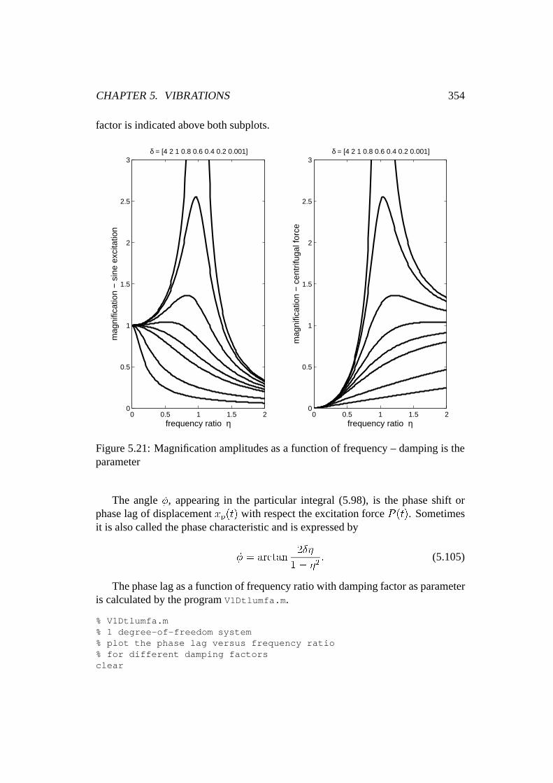
See [28] for details. The programV1Dtluma.m provides the calculation and plottingof magnification factors as functions of frequency ratio� for different values of adamping factorÆ.
% V1Dtluma.m% 1 degree-of-freedom system% plot magnification factor versus frequency ratio% for different damping factorsclear% frequency and damping rangeseta=0:0.01:3;delrange=[0.001 0.2 0.4 0.6 0.8 1.0 2 4];% sine function excitationfigure(1);i=0; vv=[0,2,0,3];subplot(1,2,1)for del=delrange % damping range loop
r=1./sqrt((1-eta.*eta).^2+(2*del*eta).^2);plot(eta,r,’k’,’linewidth’,2); axis(vv); grid; hold on;
endxlabel(’frequency ratio \it \eta’, ’fontsize’, 12);title(’\delta = [4 2 1 0.8 0.6 0.4 0.2 0.001]’);ylabel(’magnification - sine excitation’, ’fontsize’, 12)% excitation by centrifugal forcesubplot(1,2,2)for del=delrange
r=(eta.*eta)./sqrt((1-eta.*eta).^2+(2*del*eta).^2);plot(eta,r,’k’,’linewidth’,2); axis(vv); grid; hold on;
endxlabel(’frequency ratio \it \eta’, ’fontsize’, 12);title(’\delta = [4 2 1 0.8 0.6 0.4 0.2 0.001]’);ylabel(’magnification - centrifugal force’,’fontsize’,12)print V1Dtluma -deps; print V1Dtluma -dmeta% end of V1Dtluma
The output ofV1Dtluma.m is in Fig. 5.21. The range of values for the damping
CHAPTER 5. VIBRATIONS 354
factor is indicated above both subplots.
0 0.5 1 1.5 20
0.5
1
1.5
2
2.5
3
frequency ratio η
δ = [4 2 1 0.8 0.6 0.4 0.2 0.001]
mag
nific
atio
n −
sin
e ex
cita
tion
0 0.5 1 1.5 20
0.5
1
1.5
2
2.5
3
frequency ratio η
δ = [4 2 1 0.8 0.6 0.4 0.2 0.001]
mag
nific
atio
n −
cen
trifu
gal f
orce
Figure 5.21: Magnification amplitudes as a function of frequency – damping is theparameter
The angle�, appearing in the particular integral (5.98), is the phase shift orphase lag of displacementxp(t) with respect the excitation forceP (t). Sometimesit is also called the phase characteristic and is expressed by
� = arctan2�
1� �2: (5.105)
The phase lag as a function of frequency ratio with damping factor as parameteris calculated by the programV1Dtlumfa.m .
% V1Dtlumfa.m% 1 degree-of-freedom system% plot the phase lag versus frequency ratio% for different damping factorsclear

CHAPTER 5. VIBRATIONS 355
% it is plotted in two steps% since there is a singularity for eta =1
figure(1)vv=[0 3 0 pi]; % scaling% delta rangedeldiv=[0 0.01 0.1 0.3 0.5 1 2 4];eta=0:0.01:0.99; % the first part of frequency rangefor del=deldiv
arg=2*del*eta./(1-eta.*eta);fi=atan(arg);plot(eta,fi,’k’,’linewidth’,2); axis(vv); hold on
end
eta=1.01:0.01:3; % the second partfor del=deldiv
arg=2*del*eta./(1-eta.*eta);fi=atan(arg)+pi;plot(eta,fi,’k’,’linewidth’,2); axis(vv); hold on
end% plot the discontinuityx=[1 1]; y=[0 pi];plot(x,y,’k’, ’linewidth’,2);title(’\delta = [0 0.01 0.1 0.3 0.5 1 2 4]’)xlabel(’frequency ratio \it \eta’, ’fontsize’, 12);ylabel(’Phase lag \it \phi’, ’fontsize’, 12);print V1Dtlumfa -deps; print V1Dtlumfa -dmeta;% end of V1Dtlumfa.m
The output ofV1Dtlumfa.m is in Fig. 5.22.Conclusions for the steady-state motion described by the particular integral are
as follows
� the motion is harmonic, of the same frequency as excitation,
� for a given frequency and amplitude of the harmonic excitation the responseis constant,
� the motion is independent of initial conditions,
� the amplitude of the motion depends on the amplitude and the frequency ofthe excitation,
� at resonance, when the frequency ratio equals 1, the magnification factor islimited only by the damping factor,
� the excitation and the response do not attain their maximum values at thesame time. The phase lag is the measure of this difference.

CHAPTER 5. VIBRATIONS 356
0 0.5 1 1.5 2 2.5 30
0.5
1
1.5
2
2.5
3
δ = [0 0.01 0.1 0.3 0.5 1 2 4]
frequency ratio η
Pha
se la
g φ
Figure 5.22: Phase lag as a function of frequency ratio for different values of thedamping factor

CHAPTER 5. VIBRATIONS 357
5.9.4 Overdamped, critically damped and underdamped linearvibrations of a one-degree-of-freedom system
m
k
x
b
Figure 5.23: Free vibration of a damped system
For given values of massm; viscous damping coefficientb, stiffnessk, initialdisplacementx0 and initial velocityv0 find the time history of displacementx =x(t) of the particle for different values of a damping parameter. The massm issupposed to slide without friction on the ground andx is measured from the staticequilibrium position, see Fig. 5.23.
The equation of motion and usual rearrangements are
m�x = �kx� b _x;
m�x + b _x + kx = 0;
�x+b
m_x+
k
mx = 0;
�x + 2N _x +2x = 0: (5.106)
where =pk=m andN = b=(2m).
Assuming the solution in the formx = e�t we get the so-called characteristicequation in the form
�2 + 2N�+2 = 0 (5.107)
and its roots are�1;2 = �N �
pN2 � 2: (5.108)
If the roots are distinct (real or complex), then the solution of Eq. (5.106) and itsderivatives are
x = C1 e�1t + C2 e
�2t;
_x = �1 C1e�1t + �2 C2e
�2t;
�x = �21 C1e�1t + �22 C2e
�2t:
(5.109)

CHAPTER 5. VIBRATIONS 358
The unknown constants could be determined from initial conditions. Taking forexample the initial conditions such that fort = 0: x = 0 and _x = v0 we get
0 = C1 + C2 v0 = C1�1 + C2�2;
C1 =v0
�1 � �2C2 =
v0�2 � �1
: (5.110)
Substuting the constants into Eq. (5.106) we obtain for given initial conditions theexpression
x(t) =v0
�1 � �2e�1t � v0
�1 � �2e�2t
x = x(t) =v0
�1 � �2
�e�1t � e�2t
�: (5.111)
� If the roots of the characteristic equation (5.107) are real, then the motion issaid to be aperiodic. We could have either two distinct roots or one multipleroot.
– The case of two distinct roots occurs ifN > i.e. if the value of thedamping factorÆ = N= > 1. The system is said to be overdamped.
– The case of one multiple root occurs ifN = i.e. if the value ofthe damping factorÆ = N= = 1. The system is said to be criticallydamped. The solution of the equation of motion, instead of (5.109),however, must be assumed in the form
x = (C1 + C2t) e�t: (5.112)
� If the roots of the characteristic equation (5.107) are complex, then the motionis said to be periodic. The characteristic equation has complex roots ifN < or if the value of the damping factorÆ = N= < 1. In this case the system isunderdamped.
We can easily show that in case of nonzero initial displacementsx0 and veloci-tiesv0 respectively, the solution in the form
x(t) =v0 � �2x0�1 � �2
e�1t � v0 � �1x0�1 � �2
e�2t for two distinct roots, (5.113)
x(t) = [x0 + (v0 + x0)t] e�t for a multiple root. (5.114)
In case of a periodic motion the solution (5.109) is usually rewritten by meansof trigonometric function for further numerical processing. There is no necessityto do it in Matlab since Matlab can easily handle complex numbers. Actually anynumber is a priori assumed to be complex. See the programV1Otlumk1a.m and itsoutput, i.e. Fig. 5.24, where displacement as a function of time for three distinctdamping cases is plotted.
CHAPTER 5. VIBRATIONS 359
% V1Otlumk1aclear% one degree of freedom% overdamped, critically damped and underdamped system
% given datam=2; % mass of a particle [kg]l0=0.3; % length of unstretched spring [m]x0=0.1; % initial displacement [m]v0=0; % initial velocity [m/s]% range of constantsk = [288,288,288]; % stiffness [Ns/m]b = [288,2*sqrt(k(2)*m),10]; % damping [N/m]
% checkOM = sqrt(k/m);NN = b/(2*m);delta = NN./OM;t = 0:0.01:1.4; % time range
for i=1:3% constantsOM(i)=sqrt(k(i)/m); % angular frequencyif i==2, % critical damping
x=(x0+(v0+x0*OM(i))*t).*exp(-OM(i)*t);else % under- and over-critical damping
N(i)=b(i)/(2*m); % damping coefficientza(i)=N(i)^2-OM(i)^2;lam1(i)=-N(i)+sqrt(za(i));lam2(i)=-N(i)-sqrt(za(i));zl1(i)=(v0-lam2(i)*x0)/(lam1(i)-lam2(i));zl2(i)=(v0-lam1(i)*x0)/(lam1(i)-lam2(i));x=(zl1(i)*exp(lam1(i)*t))-(zl2(i)*exp(lam2(i)*t));
end % of ifmx(i,:)=x;
end % of for loop
% plotfigure(1)label1=[’overdamped, delta = ’ num2str(delta(1))];label2=[’critically damped, delta = ’ num2str(delta(2))];label3=[’underdamped, delta = ’ num2str(delta(3))];for i=1:3
subplot(3,1,i)plot(t,mx(i,:),’k’,’linewidth’,2);if i==1, text(0.6,0.07,label1);elseif i==2, text(0.6,0.07,label2);
ylabel(’displacement x [m]’);else, text(0.6,0.07,label3);xlabel(’time t [s]’);

CHAPTER 5. VIBRATIONS 360
endendprint V1Otlumk1a -dmeta; print V1Otlumk1a -deps% end of V1Otlumk1a
0 0.2 0.4 0.6 0.8 1 1.2 1.40.02
0.04
0.06
0.08
0.1
overdamped, delta = 6
0 0.2 0.4 0.6 0.8 1 1.2 1.40
0.05
0.1
critically damped, delta = 1
disp
lace
men
t x [m
]
0 0.2 0.4 0.6 0.8 1 1.2 1.4−0.1
−0.05
0
0.05
0.1underdamped, delta = 0.20833
time t [s]
Figure 5.24: Three cases of damping of a one-degree-of-freedom vibrating system

CHAPTER 5. VIBRATIONS 361
5.9.5 A vibrating system attached to a moving support
m
kz
y=y ( t)0sin ω
vibrating support
x
Figure 5.25: System excited by motion of support
Often, the motion of the support excites the dynamical system. This can beidealized by assuming a one-degree-of-freedom system in which the motion of itssupport is prescribed by a harmonic function of time as shown in Fig. 5.25.
The equation of motion of the particle is
m�x + k(x� y) = 0; (5.115)
m�x + kx = ky: (5.116)
Assuming the harmonic motion of the foundation in the form
y = y0 sin(!t) (5.117)
and defining2 = k=m we get
m�x + kx = ky0 sin(!t); (5.118)
�x+2x = 2y0 sin(!t): (5.119)
The particular solution could be assumed in the form
xp = x0 sin(!t) ) �xp = �!2x0 sin(!t): (5.120)
Substituting we get
�!2x0 sin(!t) +2x0 sin(!t) = 2y0 sin(!t): (5.121)

CHAPTER 5. VIBRATIONS 362
Realizing that this relation must be valid for any timet we can write
x0 =2
2 � !2y0: (5.122)
The steady-state motion of the particle is thus described by
x = y02
2 � !2sin(!t): (5.123)
What is of interest is the ratio of amplitudes
x0y0
=2
2 � !2=
1
1� (!=)2=
1
1� �2(5.124)
where� = != is the frequency ratio.One can notice that if� � 1, thenx0=y0 ! 0 ) x0 ! 0, which means that
the amplitude of the forced motion goes to zero. The particlem thus does not movewith respect to the ground.
Realizing that the relative motion is
z = x� y (5.125)
we can conclude that is this case the relative displacement of the particle corre-sponds to the motion of the foundation with respect to the ground, i.e.
z = �y: (5.126)
If we want the vibrating system to behave this way (� � 1) we have to set small with respect to!, i.e. the spring stiffnessk should be small with respectto massm. A system tuned this way could be used as a device for mechanicalmeasurements of relative displacements i.e, a vibrometer.
Let us express the equation of motion by means of relative coordinatesz. Insuch a case we could write
m�x + k(x� y) = 0; z = x� y: (5.127)
With 2 = k=m andy = y0 sin(!t)) �y = �!2y0 sin(!t) we get
�z +2z = !2y0 sin(!t): (5.128)
The particular integral and its second time derivative are
zp = z0 sin(!t) ) �zp = �!2z0 sin(!t): (5.129)

CHAPTER 5. VIBRATIONS 363
Substituting into the equation of motion
�!2z0 sin(!t) +2z0 sin(!t) = !2z0 sin(!t) (5.130)
and expressing the ratio of amplitudes we get
z0�2 � !2
�= !2y0 ) z0
y0=
!2
2 � !2=
�2
1� �2: (5.131)
If � � 1 thenz0=y0 ! �2 and the amplitude of the relative motion is proportionalto the acceleration of the foundationz0 = y0�
2 = y0 (!2=2). If we want frequency
ratio � � 1 then!= � 1 which requiresk being large with respect tom since =
pk=m. For such a tuning the system behaves as an accelerometer.
ProgramV1Gvibgrafa.m plots the amplitude ratio (magnification factor) versusfrequency ratio for both cases. The output is in Fig. 5.26.
% V1Gvibgrafa% plot magnification factors for vibrometer and accelerometercleareta1=0:0.01:0.99; eta2=1.01:0.01:3;v1=1./(1-eta1.^2); v2=1./(1-eta2.^2);a1=eta1.^2./(1-eta1.^2); a2=eta2.^2./(1-eta2.^2);x1=[0 3]; y1=[1 1]; x2=[1 1]; y2=[0 3];
figure(1)subplot(1,2,1);plot(eta1,v1,’r’, eta2,abs(v2),’r’, x1,y1,’:k’, x2,y2,’:k’, ...
’linewidth’, 2);axis([0 3 0 3]); axis(’square’); title(’vibrometer’);ylabel(’magnification factor’); xlabel(’frequency ratio’);subplot(1,2,2);plot(eta1,a1,’r’, eta2,abs(a2),’r’, x1,y1,’:k’, x2,y2,’:k’, ...
’linewidth’, 2);axis([0 3 0 3]); axis(’square’); xlabel(’frequency ratio’);title(’accelerometer’); ylabel(’magnification factor’);print V1Gvibgrafa -dmeta; print V1Gvibgrafa -deps;% end of V1Gvibgrafa

CHAPTER 5. VIBRATIONS 364
0 1 2 30
0.5
1
1.5
2
2.5
3vibrometer
mag
nific
atio
n fa
ctor
frequency ratio0 1 2 3
0
0.5
1
1.5
2
2.5
3
frequency ratio
accelerometerm
agni
ficat
ion
fact
or
Figure 5.26: Magnification factors for vibrometer and accelerometer

CHAPTER 5. VIBRATIONS 365
5.9.6 Behaviour of a one-degree-of-freedom linear system at res-onance
lk
x
x
h
b
mg
P t0sin ω
..
Figure 5.27: Vibrating system excited by a harmonic force
One-degree-of-freedom system, depicted in Fig. 5.27, is formed by a particleand a leaf spring. The mass of particle ism. The leaf spring stiffness (having thelengthl) is k. The system is excited by a harmonic force having the amplitudeP0
and the angular frequency!. Let’s find out what happens when the value of theexcitation frequency! approaches to that of natural frequency. For a given setof initial conditions, sayt = 0, x = 0, _x = 0, the displacement of the particle as afunction of timex = x(t) is to be determined. For a rectangular cross sectionb byh the spring stiffness is
k =3EI
l3where I =
bh3
12: (5.132)
If a small particle and small displacements with respect to equilibrium positionare considered and the influence of the weight is neglected, then the equation ofmotion could be written in the form
�x +2x =P0
msin(!t) where =
rk
m: (5.133)
The complementary function integral could be assumed in the form
xh = C sin(t + ); (5.134)
while the particular integral and its derivatives are
xp = r sin(!t) ) _xp = r! cos(!t); �xp = �r!2 sin(!t): (5.135)

CHAPTER 5. VIBRATIONS 366
Substituting the particular integral into the equation of motion we get
�r!2 sin(!t) +2r sin(!t) =P0
msin(!t); (5.136)
which must be valid for any timet, so the amplitude of the forced vibration is
r =P0=m
2 � !2: (5.137)
Thus the general solution and its derivative are
x = C sin(t+ ) +P0=m
2 � !2sin(!t)
_x = C cos(t + ) +P0=m
2 � !2! cos(!t):
(5.138)
Substituting the values of initial conditions (t = 0, x = 0, _x = 0) into the previoustwo equations we get the unknown constants
0 = C sin +P0=m
2 � !2sin (!0) ) sin = 0 ) = 0;
0 = C cos |{z}1
+P0=m
2 � !2! ) C = � P0=m
2 � !2
!
:
(5.139)
Thus the general solution is
x = � P0=m
2 � !2
!
sin(t) +
P0=m
2 � !2sin(!t) (5.140)
x =P0=m
2 � !2
hsin(!t)� !
sin(t)
i: (5.141)
The amplitude of steady-state vibration is
r =P0m
2 � !2=
P0m
12
1� !2
2
=
P0m
mk
1� !2
2
=P0
k
1
1� !2
2
; (5.142)
Any real mechanical system, however, could not reach infinite displacement im-mediately. The time history of displacements at resonance could be derived as alimiting value of Eq. (5.141) for! ! . Since the expression is of the form0=0,we can apply the l’Hôpital rule and differentiate the numerator and denominator ofthe expression with respect to!.
lim!!
x =P0
mlim!!
�sin(!t)� !
sin(t)
2 � !2
�=P0
mlim!!
�t cos(!t)� 1
sin(t)
�2!�=
=P0
m
� 1sin(t)� t cos(t)
2
�=
P0
2m
�1
sin(t)� t cos(t)
�: (5.143)

CHAPTER 5. VIBRATIONS 367
The time history of displacement is composed of two periodic motions having thesame periods. The amplitude of the cosine function increases linearly with time andwould eventually become infinite. At infinite time, however. Nature is sometimesvery kind to us. Displacements of a one-degree-of-freedom system at resonance asa function of time are depicted in Fig. 5.28 which was generated by the programV1Rkmivreza.m .
% V1Rkmivreza% vibration at resonancecleart=0:0.05:10; % time range% constants in the formula for displacementsp0=1; m=10; om=6;const=p0/(2*m*om);x=const*(sin(om*t)/om - t.*cos(om*t));figure(1)plot(t,x,’k’, ’linewidth’, 2);title(’Vibrations at resonance’);xlabel(’time’); ylabel(’displacement’);print V1Rkmivreza -deps; print V1Rkmivreza -dmeta% end of kmivreza

CHAPTER 5. VIBRATIONS 368
0 1 2 3 4 5 6 7 8 9 10−0.08
−0.06
−0.04
−0.02
0
0.02
0.04
0.06
0.08
0.1Vibrations at resonance
time
disp
lace
men
t
Figure 5.28: Vibration at resonance

CHAPTER 5. VIBRATIONS 369
5.9.7 Vibration with Coulomb friction
Let us consider a one-degree-of-freedom system according to Fig. 5.29.
mk
l0
S
N
F1 F
2mg
x
Figure 5.29: Vibration with Coulomb friction
For a given value of massm, spring stiffnessk, coefficient of frictionf , andinitial conditions fort = 0, x(0) = x0 and _x(0) = 0 the aim is to determine themotion of the mass as a function of time. The Coulomb type of friction, where thefriction force is proportional to the normal reaction, is considered.
Let us denote the motion to the right – in the positive direction ofx-axis – as1,and the opposite one as2. The equation of motion in the direction1 is
m�x = �kx� F1; (5.144)
while in the direction2 we have
m�x = �kx + F2: (5.145)
The friction forces areF1 = F2 = Nf = mgf: (5.146)
Introducing2 = k=m and rearranging we get
�x+2x = �gf: (5.147)
The solution can be assumed in the form
x = A sin (t + )� gf
2: (5.148)
The plus sign holds for the motion in the direction2, the minus sign for direction1.For the prescribed initial conditions, given above, the motion in the direction2
will come up first. Then the particle displacement and velocity allow expressing theunknown constants
x = A sin (t + ) +gf
2; ) x0 = A sin +
gf
2; (5.149)
_x = A cos (t + ) ) 0 = A cos : (5.150)

CHAPTER 5. VIBRATIONS 370
So
cos = 0 ) =�
2; (5.151)
x0 = A+gf
2) A = x0 � gf
2: (5.152)
Introducing
p =gf
2(5.153)
for the first half-period we can write
x = (x0 � p) cos (t) + p: (5.154)
At the end of the first half-periodt1 = T=2 = �= the particle stops and begins tomove to the right (direction1) with new initial conditions, i.e.
x(t1) = (x0 � p) cos
��
�+ p = � (x0 � 2p) ; (5.155)
_x (t1) = 0: (5.156)
Now, the displacement of the particle for motion in the direction1 is
x = A sin (t + )� p: (5.157)
Substituting the new initial conditions (5.155), (5.156) in the equation of motion(5.157) and into its time derivative
_x = A cos (t + ) (5.158)
we get new integration constants valid for the second half-period, namely
cos = 0 ) =�
2; (5.159)
� x0 + 2p = A� p ) A = � (x0 � 3p) : (5.160)
So the displacement of the particle for motion in the direction1 is
x = � (x0 � 3p) cos (t)� p: (5.161)
One should notice that timet is measured fromt1 from now on. The reader shouldprove that for another half-period the particle displacement is described by
x = (x0 � 4p) cos (t + ) + p: (5.162)
ProgramVCFkmitren.m takes care of evaluating the above-derived formulas.

CHAPTER 5. VIBRATIONS 371
% VCFkmitren% Vibration with Coulomb frictionclear% input datag = 9.81; % gravity accelerationm = 2; % massk = 6; % spring stiffnessf = 0.15; % coefficient of Coulomb frictionx0 = 5; % initial displacementi = 0; % half-period counter
% Computation itselfo = k/m; % OMEGA squaredom = sqrt(o); % OMEGA ... natural frequencyp = g*f/o;T = 2*pi/om; % periodtt = 0:pi/64:6*pi; % time rangefor t=tt;
i = i+1; jj(i) = fix(2*t/T)+1;j = jj(i);if rem(j,2) == 0,
d=p;else
d=0;endv(i)=(x0-p)*om*sin(om*t);ww(i)=VCFmojesig(v(i));w=ww(i);ampl=x0-j*p;if ampl >= p,
x(i)=w*(x0-j*p)*cos(om*(t-(j-1)*T/2))+w*p+d;else
x(i)=0;end
end
% p linesupdisp = [p p];lodisp = [-p -p];tm = [0 6*pi];
figure(1)plot(tt,x,’r’, tm,updisp,’:k’, tm,lodisp,’:k’,’linewidth’,2);xlabel(’time [s]’,’fontsize’, 12);ylabel(’displacement [m]’,’fontsize’, 12);title(’Vibration with Coulomb friction’,’fontsize’, 12);print VCFkmitren -deps; print VCFkmitren -dmeta;
% end of VCFknitren.m
function w=VCFmojesig(v);

CHAPTER 5. VIBRATIONS 372
if v>=0,w=1;else w=-1;end
% end of VCFmojesig
The graphical output of this program is in Fig. 5.30.
0 2 4 6 8 10 12 14 16 18 20−5
−4
−3
−2
−1
0
1
2
3
4
5
time [s]
disp
lace
men
t [m
]
Vibration with Coulomb friction
Figure 5.30: Displacement of a particle under the influence of Coulomb friction
One should notice that the amplitudes of vibration decrease linearly; the motionstops sometime after the amplitude of displacement becomes less than�p.

CHAPTER 5. VIBRATIONS 373
5.10 Systems with 2 DOF
5.10.1 Undamped free and forced vibrations of a two-degrees-of-freedom linear system
m1
m2
k1
k2
x1
x2
s1
s2
s2
Figure 5.31: A two-degree-of-freedom system
The equations of motions are
m1�x1 = �S1 + S2;
m2�x2 = �S2:(5.163)
The spring forces are proportional to their extensions
S1 = k1x1;
S2 = k2(x2 � x1):(5.164)
Substituting, rearranging
m1�x1 = �k1x1 + k2(x2 � x1);
m2�x2 = �k2(x2 � x1):(5.165)
m1�x1 + x1(k1 + k2) + x2(�k2) = 0;
m2�x2 + x1(�k2) + x2(k2) = 0:(5.166)
and rewriting into the matrix form�m1 00 m2
���x1�x2
�+
�k1 + k2 �k2�k2 k2
��x1x2
�=
�00
�(5.167)
we finally get[M ] f�xg+ [K] fxg = f0g (5.168)

CHAPTER 5. VIBRATIONS 374
where[M ], [K] are mass and stiffness matrices respectively. These equations arelinear and homogeneous of the second order and their solutions can be assumed inthe form
x1 = C1 sin(t + )
x2 = C2 sin(t + )
))
�x1 = �2C1 sin(t + );
�x2 = �2C2 sin(t + ):(5.169)
Substituting into the equations of motion and ’dividing out by the sine function’ weget
�m1C12 = �k1C1 + k2(C2 � C1);
�m2C22 = �k2(C2 � C1):
(5.170)
C1(�m12 + k1 + k2) + C2(�k2) = 0;
C1(�k2) + C2(�m22 + k2) = 0:
(5.171)
This is a set of homogeneous linear algebraic equations inC1 andC2, whichhave a nontrivial solution only if the determinant of the coefficient vanishes, that is���� �m1
2 + k1 + k2 �k2�k2 �m2
2 + k2
���� = 0: (5.172)
This is called the characteristic - or the - frequency equation of the system fromwhich the values of natural frequencies can be determined. Solving the frequencyequation we get
1;2 =
vuut1
2
�k1 + k2m1
+k2m2
��s
1
4
�k1 + k2m1
+k2m2
�2
� k1k2m1m2
: (5.173)
The natural frequencies, also called eigenfrequencies, can be found by Matlabboth analytically and numerically.
Generally, the eigenfrequencies of a mechanical system withn degrees of free-dom described by
[M ] f�xg+ [K] fxg = f0g (5.174)
could be found assuming
fxg = fx0g eit ) f�xg = �2 fx0g eit: (5.175)
Substituting the assumed vibrations into the equation of motion we get a so-called generalized eigenvalue problem
([K]� [M ]) fx0g = f0g ; (5.176)

CHAPTER 5. VIBRATIONS 375
that could be transformed into a standard eigenvalue problem0B@[M ]�1 [K]| {z }
[C]
�� [I]
1CA fx0g = f0g where � = 2: (5.177)
In both cases the problem is to findn couples(i; fx0gi) or (�i; fx0gi) satisfy-ing the above equations.
Matlab can solve both problems numerically; for analytical solution, however,only the standard eigenvalue problem can be treated by the Matlab symbolic tool-box. See the programV2Etwodofa.m .
% V2Etwodofaclear; format compact% find eigenfrequencies of a two-degrees-of freedom system% the set of equations is%% m1*D2x1=-k1*x1+k2*(x2-x1)% m2*D2x2=-k2*(x2-x1)%% add a - symbolic approach% mass matrix
% numerical values arem1=400; m2=300; k1=60000; k2=50000;
m=sym(’[m1,0;0,m2]’);% stiffness matrixk=sym(’[k1+k2,-k2;-k2,k2]’);% transform it into a standard eigenvalue problemminv = inv(m);c=sym(minv)*sym(k);
ei=eig(c); % calculate eigenvaluesdisp(’the formula for the first eigenvalue is’)la1s=sym(ei,1,1)disp(’the source code for TEX processing’)latex(la1s) % source code for TEX processing - just for funla2s=sym(ei,2,1); % and this is the second one, do not print itdisp(’evaluate numerically the formula derived by Matlab’)disp(’eigenfrequencies are square roots of eigenvalues’)
einumeric = sqrt(subs(ei))
% add b - a classical numeric approachdisp(’evaluate numerically the formula (5.173) derived in the text’)a=(k1+k2)/m1;b=k2/m2;

CHAPTER 5. VIBRATIONS 376
c=k1*k2/(m1*m2);% print the resultsom1=sqrt(0.5*(a+b)+sqrt(0.25*(a+b)^2-c))om2=sqrt(0.5*(a+b)-sqrt(0.25*(a+b)^2-c))disp(’The results are the same - what else could you expect?’)% end of V2Etwodofa
The text output of this program is
>> V2Etwodofathe formula for the first eigenvalue isla1s =1/2/m1/m2*(k1*m2+k2*m2+m1*k2+(k1^2*m2^2+2*k1*m2^2*k2-2*k1*m2*m1*k2+k2^2*m2^2+2*k2^2*m2*m1+m1^2*k2^2)^(1/2))the source code for TEX processingans =1/2\,{\frac {{\it k1}\,{\it m2}+{\it k2}\,{\it m2}+{\it m1}\,{\it k2}+\sqrt {{{\it k1}}^{2}{{\it m2}}^{2}+2\,{\it k1}\,{{\it m2}}^{2}{\it k2}-2\,{\it k1}\,{\it m2}\,{\it m1}\,{\it k2}+{{\it k2}}^{2}{{\it m2}}^{2}+2\,{{\it k2}}^{2}{\it m2}\,{\it m1}+{{\it m1}}^{2}{{\it k2}}^{2}}}{{\it m1}\,{\it m2}}}evaluate numerically the formula derived by Matlabnotice that eigenfrequencies are square roots of eigenvalueseinumeric =
19.36498.1650
evaluate numerically the formula (5.173) derived in the textom1 =
19.3649om2 =
8.1650The results are the same - what else could you expect?>>
The complementary function satisfying the equations of motion could be writtenin an alternative form
x1 = C11 sin (1t+ 1) + C12 sin (2t+ 2) ;
x2 = C21 sin (1t+ 1) + C22 sin (2t+ 2) :(5.178)
Since (5.171) is a set of homogeneous equations we can obtain the ratio of ampli-

CHAPTER 5. VIBRATIONS 377
tudes and express them for both natural frequencies obtained from (5.173)
C2
C1=�m1
2 + k1 + k2k2
(5.179)�C2
C1
�1
=�m1
21 + k1 + k2k2
(5.180)�C2
C1
�2
=�m1
22 + k1 + k2k2
(5.181)
C2
C1=
k2�m22 + k2
(5.182)�C2
C1
�1
=k2
�m221 + k2
(5.183)�C2
C1
�2
=k2
�m222 + k2
: (5.184)
From the four ratios defined by (5.180), (5.181), (5.183) and (5.184) only two areindependent. Defining�
C2
C1
�1
= �21;
�C2
C1
�2
= �22 (5.185)
we could setC21 = �21C11; C22 = �22C12: (5.186)
Finally, the equation (5.178), describing the transient response of the system, canbe rewritten into
x1 = C11 sin (1t+ 1) + C12 sin (2t+ 2) ;
x2 = �21C11 sin (1t+ 1) + �22C12 sin (2t + 2) :(5.187)
The unknown constantsC11, C12, 1, 2 can be determined from initial conditionsas it is shown in 5.10.2.
Forced vibrations of a two-degrees-of-freedom systemIf a harmonic excitation of the same frequency and of the same phase is applied
to both particles, then the equations of motion are
m1�x1 + k1x1 � k2 (x2 � x1) = P1 sin (!t)
m2�x2 + k2 (x2 � x1) = P2 sin (!t) :(5.188)
The particular integrals, describing the steady-state response of the system, couldbe assumed in the form
x1 = A1 sin(!t) ) �x1 = �!2A1 sin(!t);
x2 = A2 sin(!t) ) �x2 = �!2A2 sin(!t):(5.189)
CHAPTER 5. VIBRATIONS 378
Substituting into the equations of motion we get
�m1A1!2 + k1A1 � k2 (A2 � A1) = P1;
�m2A2!2 + k2 (A2 � A1) = P2;
(5.190)
� �m1!2 + k1 + k2 �k2�k2 �m2!
2 + k2
��A1
A2
�=
�P1
P2
�: (5.191)
The amplitudes are
A1 =P1 (k2 �m2!
2) + P2k2(k1 + k2 �m1!2) (k2 �m2!2)� k22
;
A2 =P2 (k1 + k2 �m2!
2) + P1k2(k1 + k2 �m1!2) (k2 �m2!2)� k22
:
(5.192)
Read carefully the programtwodof2a.m where three different approaches to thedetermination of amplitudes of the steady-state motion are compared
% V2Etwodof2a% forced vibration of a two-degrees-of-freedom system
% m1*D2x1+k1*x1-k2*(x2-x1)=p1*sin(om*t)% m2*D2x2 +k2*(x2-x1)=p2*sin(om*t)
% numerical valuesclearm1=400; m2=300; k1=60000; k2=50000;om=5; p1=10; p2=15;
% assuming the solution% x1=a1*sin(om*t)% x2=a2*sin(om*t)% and substituting it into Eq. of motion% we get a system of algebraic equations% where the matrix is
ms=sym(’[-m1*om^2+k1+k2,-k2;-k2,-m2*om^2+k2]’);ims=inv(ms);% and the right-hand side vector isp=sym(’[p1;p2]’);% the symbolic solution for amplitudes isa=symmul(ims,p);% extract componentsdisp(’the first amplitude’)a1a=sym(a,1,1)disp(’the second amplitude’)a2a=sym(a,2,1)disp(’their numeric values are’)

CHAPTER 5. VIBRATIONS 379
a1an=subs(a1a)a2an=subs(a2a)
% an alternative approach
aalter=linsolve(ms,p);disp(’numeric values found by an alternative way’)aalter1n=eval(sym(aalter,1,1))aalter2n=eval(sym(aalter,2,1))
disp(’evaluate numerically the formula (5.192)’)jm=(k1+k2-m1*om^2)*(k2-m2*om^2)-k2^2;a1=(p1*(k2-m2*om^2)+p2*k2)/jma2=(p2*(k1+k2-m1*om^2)+p1*k2)/jm
% plot time history of displacementst=0:0.01:10;x1=a1*sin(om*t);x2=a2*sin(om*t);figure(1)subplot(2,1,1); plot(t,x1,’linewidth’,2);title(’the first particle displacement’,’fontsize’, 12);subplot(2,1,2); plot(t,x2,’linewidth’,2);title(’the second particle displacement’,’fontsize’, 12);xlabel(’time’,’fontsize’, 12)print V2Etwodof2a -deps; print V2Etwodof2a -dmeta% end of V2Etwodof2a
The text output of the program is
>> V2Etwodof2athe first amplitudea1a =-(m2*om^2-k2)/(m1*om^4*m2-m1*om^2*k2-k1*m2*om^2+k1*k2-k2*m2*om^2)*p1+k2/(m1*om^4*m2-m1*om^2*k2-k1*m2*om^2+k1*k2-k2*m2*om^2)*p2the second amplitudea2a =k2/(m1*om^4*m2-m1*om^2*k2-k1*m2*om^2+k1*k2-k2*m2*om^2)*p1-(m1*om^2-k1-k2)/(m1*om^4*m2-m1*om^2*k2-k1*m2*om^2+k1*k2-k2*m2*om^2)*p2their numeric values area1an =
6.7143e-004a2an =
0.0011numeric values found by an alternative wayaalter1n =
6.7143e-004aalter2n =

CHAPTER 5. VIBRATIONS 380
0.0011evaluate numerically the formula (5.192)a1 =
6.7143e-004a2 =
0.0011>>
The graphical output is in Fig. 5.32 and is not too interesting
0 1 2 3 4 5 6 7 8 9 10−1
−0.5
0
0.5
1x 10
−3 the first particle displacement
0 1 2 3 4 5 6 7 8 9 10−1.5
−1
−0.5
0
0.5
1
1.5x 10
−3 the second particle displacement
time
Figure 5.32: Forced vibration of a two-degrees-of-freedom system
Solution by means of the Newmark integration method.Time history of the response of more complicated mechanical systems with
many degrees of freedom is usually found numerically. A number of integrationmethods are available. One of them, very popular in technical practice, is the socalled Newmark integration method. Let us apply the Newmark method for the me-chanical system described in the text above and in the programV2Etwodof3a.m andcompare the time history of displacements of both particles. Numerical integrationis provided by the functionV2Enewmd.m. See paragraph 5.8.2.

CHAPTER 5. VIBRATIONS 381
% V2Etwodof3a.mclear% Newmark method employed for the integration of% a two-degree-of-freedom system - same as in V2Etwodof2a.m
% numerical valuesm1=400; m2=300; k1=60000; k2=50000;om=5; p10=10; p20=15;tmax=10; % maximum value of timeh=0.02; % time steptt=0:h:tmax; % time range
xm=[m1 0; 0 m2]; % mass matrixxk=[k1+k2 -k2; -k2 k2]; % stiffness matrix
% numerical solution% Newmark method parametersgama=0.9; beta=0.25*(0.5+gama)^2;a1=1/(beta*h*h);a1d=gama/(beta*h);ck=0; cm=0; % damping coefficientsxd=ck*xk+cm*xm; % damping matrixp=[0 0]’; % initial forcesxk=xk+a1*xm+a1d*xd; % effective. stiff. matrixacc=xm\p; % initial accelerationdis=zeros(2,1); % initial displacementsvel=zeros(2,1); % initial velocitiest=0; % initial timekk=0; % step counterkmax=round(tmax/h); % how many steps for tmax
% dimensions of arrays to be plotted laterdis1=zeros(kmax,1);dis2=zeros(kmax,1);
while t<=tmax, % integate while t <= tmax[disn,veln,accn] = ...
VTRnewmd(beta,gama,dis,vel,acc,xm,xd,xk,p,h);kk=kk+1; % increment step countert=t+h; % increment time valuedis1(kk)=dis(1); dis2(kk)=dis(2); % save for plottingdis=disn; vel=veln; acc=accn; % new values for next stepp1=p10*sin(om*t); p2=p20*sin(om*t); % excitation forcesp=[p1 p2]’;
end;
% analytical solution% amplitudes of steady-state motion according to Eq. (5.192)jm=(k1+k2-m1*om^2)*(k2-m2*om^2)-k2^2;

CHAPTER 5. VIBRATIONS 382
am1=(p10*(k2-m2*om^2)+p20*k2)/jm;am2=(p20*(k1+k2-m1*om^2)+p10*k2)/jm;% calculate steady-state response% displacements according to (5.182) arex1=am1*sin(om*tt);x2=am2*sin(om*tt);dis1t=dis1’; dis2t=dis2’;
% compare results - plot itfigure(1)
subplot(211); plot(tt(1:kmax),dis1t(1:kmax),’k:’, ...tt,x1,’k’, ’linewidth’, 2);
lab=’Steady-state (solid) vs. transient + steady-state (dotted)’;title(lab)ylabel(’particle 1’)subplot(212); plot(tt(1:kmax),dis2t(1:kmax),’k:’, ...
tt,x2,’k’, ’linewidth’, 2);lab=[’gamma for Newmark is ’ num2str(gama)];title(lab); xlabel(’time’); ylabel(’particle 2’)sgama = gama*100;str_sgama = int2str(sgama);file_name = [’V2Etwodof3a’ str_sgama];print(’-deps’, file_name); print(’-dmeta’, file_name);% print V2Etwodof3a -deps; print V2Etwodof3a -dmeta;% end of V2Etwodof3a
function [disn,veln,accn] = ...VTRnewmd(beta,gama,dis,vel,acc,xm,xd,xk,p,h)
% Newmark integration method%% beta, gama coefficients% dis,vel,acc displacements, velocities, accelerations% at the begining of time step% disn,veln,accn corresponding quantities at the end% of time step% xm,xd mass and damping matrices% xk effective rigidity matrix% p loading vector at the end of time step% h time step%% constantsa1=1/(beta*h*h);a2=1/(beta*h);a3=1/(2*beta)-1;a4=(1-gama)*h;a5=gama*h;a1d=gama/(beta*h);a2d=gama/beta-1;

CHAPTER 5. VIBRATIONS 383
a3d=0.5*h*(gama/beta-2);% effective loading vectorr = p + ...
xm*(a1*dis+a2*vel+a3*acc)+xd*(a1d*dis+a2d*vel+a3d*acc);% solve system of equations for displacements xkdisn=xk\r;% new velocities and accelerationsaccn=a1*(disn-dis)-a2*vel-a3*acc;veln=vel+a4*acc+a5*accn;% end of VTRnewmd
Two graphical outputs are presented here.In Fig. 5.33 you can notice that the analytical and numerical solutions differ sig-
nificantly. This is quite clear because the former describes the steady-state responseonly, while the latter corresponds to the general solution comprising both transientand steady state solutions. It is easy to add the analytical part of the transient solu-tion and compare the results. See paragraph 5.10.2. It is, however, the steady-statepart of the response that is usually of interest in solving the engineering vibrationproblems.
The second graphical output, in Fig. 5.34, shows how the Newmark integrationmethod could be used for the removal of the transient part of solution. No numer-ical damping was introduced (gamma = 0.5) for the calculation presented in Fig.5.33. Employing the Newmark numerical damping by settinggamma = 0.9, wecan notice that the transient part of the solution quickly dies out.
More details about methods for numerical integration could be found in 5.8.2.

CHAPTER 5. VIBRATIONS 384
0 1 2 3 4 5 6 7 8 9 10−1.5
−1
−0.5
0
0.5
1
1.5x 10
−3 Steady−state (solid) vs. transient + steady−state (dotted)
part
icle
1
0 1 2 3 4 5 6 7 8 9 10−2
−1
0
1
2x 10
−3 gamma for Newmark is 0.5
time
part
icle
2
Figure 5.33: Steady-state and transient results are compared – no numerical damp-ing

CHAPTER 5. VIBRATIONS 385
0 1 2 3 4 5 6 7 8 9 10−1
−0.5
0
0.5
1x 10
−3 Steady−state (solid) vs. transient + steady−state (dotted)
part
icle
1
0 1 2 3 4 5 6 7 8 9 10−2
−1.5
−1
−0.5
0
0.5
1
1.5x 10
−3 gamma for Newmark is 0.9
time
part
icle
2
Figure 5.34: Steady-state and transient results are compared – Newmark numericaldamping

CHAPTER 5. VIBRATIONS 386
5.10.2 Comparison of analytical and numerical approaches tothe solution of the transient response of a two-degrees-of-freedom linear system
At first, let’s determine the unknown constants appearing in expression (5.187) forthe time distribution of displacements for both particles as a function of initial con-ditions. To facilitate the task it is expedient to rewrite the equations into an equiva-lent form, namely
x1 = A sin (1t) + B cos (1t) + C sin (2t) +D cos (2t)
x2 = A�21 sin (1t) +B�21 cos (1t) + C�22 sin (2t) +D�22 cos (2t) :(5.193)
Time derivatives of these equations are
_x1 = A1 cos (1t)� B1 sin (1t) + C2 cos (2t)�D2 sin (2t)
_x2 = A1�21 cos (1t)� B1�21 sin (1t) + C2�22 cos (2t)�D2�22 sin (2t) :
(5.194)
Substituting a particular set of initial conditions,t = 0: fx0g =
�x10x20
�, f _x0g =�
_x10_x20
�=
�v10v20
�into previous four equations we get the system of algebraic
equations 2664
0 1 0 10 �21 0 �22
1 0 2 0�211 0 �222 0
37758>><>>:
ABCD
9>>=>>; =
8>><>>:
x10x20v10v20
9>>=>>; (5.195)
allowing us to express the constantsA, B, C, D. A simple Matlab program, wherewe denotedki = �21, kj = �22 andom1= 1, om2= 2, will solve the task.
% V2Cinicon1clear% derive formulas for unknown constants% in Eq. (5.187) of paragraph 5.10.1% depending on initial conditions% and on omega1, omega2, k1, k2format compact% displacementsx1 = ...sym(’a*sin(om1*t)+b*cos(om1*t)+c*sin(om2*t)+d*cos(om2*t)’);x2 = sym(...’a*ki*sin(om1*t)+b*ki*cos(om1*t)+c*kj*sin(om2*t)+d*kj*cos(om2*t)’);% velocitiesv1=diff(x1,’t’);

CHAPTER 5. VIBRATIONS 387
v2=diff(x2,’t’);% substitute boundary conditionsx10=subs(x1,’0’,’t’)x20=subs(x2,’0’,’t’)v10=subs(v1,’0’,’t’)v20=subs(v2,’0’,’t’)% solve equation (5.194)s=sym(’[0,1,0,1; 0,k1,0,k2; o1,0,o2,0; k1*o1,0,k2*o2,0]’);rhs=sym(’[x10;x20;v10;v20]’);disp(’constants derived by Matlab’)x=linsolve(s,rhs)% check it numerically% initial conditionx10=1; x20=2; v10=3; v20=4;% frequencies from Eq. (5.173)o1=7; o2=8;% ratios from (5.180) and (5.184)k1=5; k2=6;
% evaluate numerically formulas derived by Matlaba=eval(sym(x,1,1));b=eval(sym(x,2,1));c=eval(sym(x,3,1));d=eval(sym(x,4,1));disp(’numerically evaluated formulas derived by Matlab’)[a b c d]
disp(’a check it numerically by "hand" ’)snum=[0,1,0,1; 0,k1,0,k2; o1,0,o2,0; k1*o1,0,k2*o2,0];rhsn=[x10;x20;v10;v20];xnum=snum\rhsn;xnum’% end of V2Cinicon1
The output of the program is
>> V2Cinicon1x10 =a*sin(om1*0)+b*cos(om1*0)+c*sin(om2*0)+d*cos(om2*0)x20 =a*ki*sin(om1*0)+b*ki*cos(om1*0)+c*kj*sin(om2*0)+d*kj*cos(om2*0)v10 =a*cos(om1*0)*om1-b*sin(om1*0)*om1+c*cos(om2*0)*om2-d*sin(om2*0)*om2v20 =a*ki*cos(om1*0)*om1-b*ki*sin(om1*0)*om1+c*kj*cos(om2*0)*om2-d*kj*sin(om2*0)*om2constants derived by Matlabx =[ -(-v20+k2*v10)/o1/(k1-k2)]

CHAPTER 5. VIBRATIONS 388
[ -(-x20+x10*k2)/(k1-k2)][ (-v20+v10*k1)/o2/(k1-k2)][ (k1*x10-x20)/(k1-k2)]numerically evaluated formulas derived by Matlabans =
2.0000 4.0000 -1.3750 -3.0000a check it numerically by "hand"ans =
2.0000 4.0000 -1.3750 -3.0000>>
The derived constants were pasted into the programV2Ctwodof5c.m and usedfor the evaluation of eqs. (5.193) describing the time distributions of both particledisplacements. The results are compared with those obtained by numerical solutionsof equations of motion (5.167). The programV2Ctwodof5c.m uses the Newmarkmethod (see the functionVTRnewmd.m) and the method of central differences (seethe functionVTRcedif.m ).
The comparison of results is presented on the following pages. There are severalidentifiers accompanying the figures, namely
gamma is the Newmark ’damping’ parameter,h is the integration step,om1 is the first frequency1,om2 is the second frequency2,tmin is the critical time step for central difference method,
i.e. tmin = 2=!max,tminmode is the period of the maximum frequency,
i.e. Tminmode = 2�=!max,hmts is the variable showing How Many Time Steps are carried out
within the period of the maximum frequency.The Fig. 5.35 shows the data obtained with time steph = 0:1 which is clearly
unreasonable. The results are shown here to ’prove’ that the Newmark method withgamma= 0:5, as a representative of unconditionally stable implicit methods, doesnot fail using too big time steps; it gives the results, however, in which the contentsof high frequency components are evidently filtered-out. But what else could weexpect when marching in time in steps that are twice as big as the period of thefastest harmonics. See the value ofhmts parameter which is of the order of 0.5. Itshould be emphasized that the notion of unconditional stability has no relation tothe precision of results. The method of central differences – as a representative ofconditionally explicit methods – fails. It simply numerically explodes – since theused time step is substantially greater than the critical time steptmin .
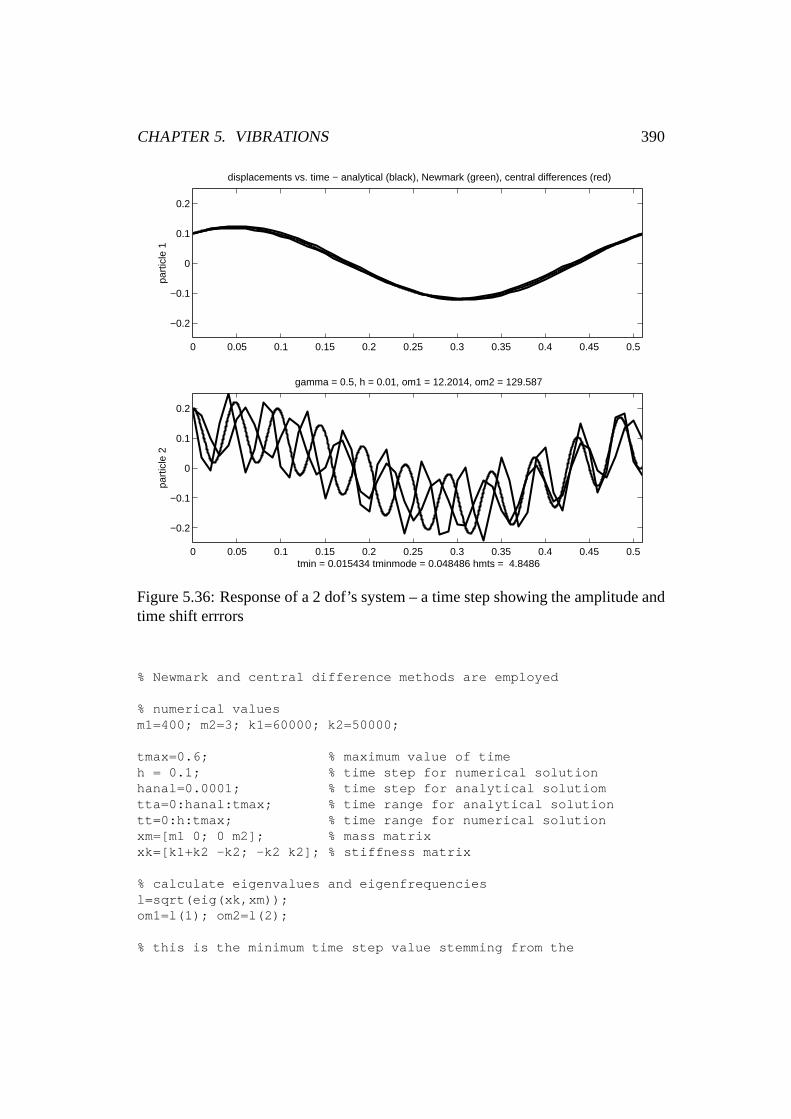
Figure 5.36 shows the data obtained with time steph = 0:01. The errors of nu-merical solutions are smaller, but there is still visible a phase shift error of oppositesigns for both numerical integration methods as before.

CHAPTER 5. VIBRATIONS 389
0 0.05 0.1 0.15 0.2 0.25 0.3 0.35 0.4 0.45 0.5
−0.2
−0.1
0
0.1
0.2
displacements vs. time − analytical (black), Newmark (green), central differences (red)
part
icle
1
0 0.05 0.1 0.15 0.2 0.25 0.3 0.35 0.4 0.45 0.5
−0.2
−0.1
0
0.1
0.2
gamma = 0.5, h = 0.1, om1 = 12.2014, om2 = 129.587
tmin = 0.015434 tminmode = 0.048486 hmts = 0.48486
part
icle
2
Figure 5.35: Transient response of a 2 dof’s system – the step of integration is toobig
Finally, Fig. 5.37 presents the results calculated with time steph = 0:001.This time, of about 50 time steps are carried out within the period of the fastestharmonics.
If we make the time step smaller and smaller, the errors of numerical integrationcould be made almost infinitely negligeable. There are two practical limits, how-ever. One is a unit round-off error, the other consists of economic considerations.
Notice that both methods of integration give reasonably accurate results if thetime step is correctly set, that is, if it is substantially smaller than the period of themaximum frequency. From this point of view there is no way to proclaim that eitherof two method is better or worse.
ProgramV2Ctwodof5c.m is as follows
% V2Ctwodof5c.mclear% comparison of analytical and two numerical solutions for% a two-degree-of-freedom system - same as in V2Ctwodof2a.m
CHAPTER 5. VIBRATIONS 390
0 0.05 0.1 0.15 0.2 0.25 0.3 0.35 0.4 0.45 0.5
−0.2
−0.1
0
0.1
0.2
displacements vs. time − analytical (black), Newmark (green), central differences (red)
part
icle
1
0 0.05 0.1 0.15 0.2 0.25 0.3 0.35 0.4 0.45 0.5
−0.2
−0.1
0
0.1
0.2
gamma = 0.5, h = 0.01, om1 = 12.2014, om2 = 129.587
tmin = 0.015434 tminmode = 0.048486 hmts = 4.8486
part
icle
2
Figure 5.36: Response of a 2 dof’s system – a time step showing the amplitude andtime shift errrors
% Newmark and central difference methods are employed
% numerical valuesm1=400; m2=3; k1=60000; k2=50000;
tmax=0.6; % maximum value of timeh = 0.1; % time step for numerical solutionhanal=0.0001; % time step for analytical solutiomtta=0:hanal:tmax; % time range for analytical solutiontt=0:h:tmax; % time range for numerical solutionxm=[m1 0; 0 m2]; % mass matrixxk=[k1+k2 -k2; -k2 k2]; % stiffness matrix
% calculate eigenvalues and eigenfrequenciesl=sqrt(eig(xk,xm));om1=l(1); om2=l(2);
% this is the minimum time step value stemming from the

CHAPTER 5. VIBRATIONS 391
0 0.05 0.1 0.15 0.2 0.25 0.3 0.35 0.4 0.45 0.5
−0.2
−0.1
0
0.1
0.2
displacements vs. time − analytical (black), Newmark (green), central differences (red)
part
icle
1
0 0.05 0.1 0.15 0.2 0.25 0.3 0.35 0.4 0.45 0.5
−0.2
−0.1
0
0.1
0.2
gamma = 0.5, h = 0.001, om1 = 12.2014, om2 = 129.587
tmin = 0.015434 tminmode = 0.048486 hmts = 48.4862
part
icle
2
Figure 5.37: Transient response of a 2 dof’s system – extremely small step
% stability consideration of the central difference methodtmin=2/max(l)% this the period of fastest modetminmode=2*pi/max(l)% how many time steps in the period of the fastest modehmts = tminmode/h
% numerical solution
% Newmark method parametersgama=0.5; beta=0.25*(0.5+gama)^2;a1=1/(beta*h*h); a1d=gama/(beta*h);
% central difference method parametersa0c=1/(h*h); a1c=1/(2*h);a2c=2*a0c; a3c=1/a2c;
ck=0; cm=0; % damping coefficientsxd=ck*xk+cm*xm; % damping matrix

CHAPTER 5. VIBRATIONS 392
p=[0 0]’; % initial forces
% effective matricesxke=xk + a1*xm + a1d*xd;% effective stiff. matrix for Newmarkxme=a0c*xm + a1c*xd; % effective mass matrix for central dif.
acc=xm\p; % initial acceleration for N.accc=xm\p; % initial acceleration for cd.
x10=0.1; x20=0.2; % initial displacementsdis=[x10; x20]; % Newmark variablesdisc=[x10; x20]; % c.d. variables
v10=0.8; v20=0.2; % initial velocitiesvel=[v10; v20]; % Newmark variablesvelc=[v10; v20]; % cd variables% displacement at time t - h for cd onlydissc = disc - h*velc + a3c*accc;
t=0; % initial timekk=0; % step counterkmax=round(tmax/h); % how many steps for tmax
% dimensions of arrays to be plotted laterdis1=zeros(kmax,1); % N. variablesdis2=zeros(kmax,1);dis1c=zeros(kmax,1); % c.d. variablesdis2c=zeros(kmax,1);
% integration loopwhile t<=tmax, % integrate while t <= tmax
[disn,veln,accn] = ...VTRnewmd(beta,gama,dis,vel,acc,xm,xd,xke,p,h);
[disnc,velnc,accnc] = ...VTRcedif(disc,dissc,velc,accc,xm,xme,xk,xd,p,h);
kk=kk+1; % increment step countert=t+h; % increment time value% save N. values for plottingdis1(kk) =dis(1); dis2(kk)=dis(2);% save c.d. values for plottingdis1c(kk)=disc(1); dis2c(kk)=disc(2);% new N. values for next stepdis=disn; vel=veln; acc=accn;% new c.d. values for next stepdissc=disc; disc=disnc; velc=velnc; accc=accnc;
end;
% analytical solution% coefficients from Eq. (5.180), (5.184)

CHAPTER 5. VIBRATIONS 393
ki=(-m1*om1^2+k1+k2)/k2;kj=k2/(-m2*om2^2+k2);
% amplitudes as derived by Matlab - V2Cinicon1.ma=-(-v20+v10*kj)/om1/(ki-kj);b= -(-x20+x10*kj)/(ki-kj);c= (-v20+ki*v10)/om2/(ki-kj);d= (ki*x10-x20)/(ki-kj);
% displacements according to (5.187) arex1=a*sin(om1*tta)+ b*cos(om1*tta)+ ...
c*sin(om2*tta)+ d*cos(om2*tta);x2=a*ki*sin(om1*tta)+b*ki*cos(om1*tta)+ ...
c*kj*sin(om2*tta)+d*kj*cos(om2*tta);
% compare results - plot itdis1t=dis1’; dis2t=dis2’;dis1tc=dis1c’; dis2tc=dis2c’;figure(1)vv = [0 0.51 -0.25 0.25];subplot(2,1,1);plot(tt(1:kmax),dis1t(1:kmax),’g’, tta,x1,’k’, ...
tt(1:kmax),dis1tc(1:kmax),’r’,’linewidth’,2);axis(vv);l1 = ’displacements vs. time - analytical (black),’;l2 = ’ Newmark (green), central differences (red)’;lab0 = [l1 l2];title(lab0);ylabel(’particle 1’)subplot(2,1,2);plot(tt(1:kmax),dis2t(1:kmax),’g’, tta,x2,’k’, ...
tt(1:kmax),dis2tc(1:kmax),’r’,’linewidth’, 2);axis(vv);lab=[’gamma = ’ num2str(gama) ’, h = ’ num2str(h) ...’, om1 = ’ num2str(om1) ’, om2 = ’ num2str(om2)];lab1=[’tmin = ’ num2str(tmin) ’ tminmode = ’ ...
num2str(tminmode) ’ hmts = ’ num2str(hmts)];title(lab); xlabel(lab1); ylabel(’particle 2’)
str_h = num2str(1000*h);file_name = [’V2Ctwodof5c’ str_h];print (’-dmeta’, file_name);print(’-deps’, file_name);
% end of V2Ctwodof5c

CHAPTER 5. VIBRATIONS 394
5.11 Systems withn DOF
5.11.1 Vibration of a linear system withn degrees of freedom
Let us consider a rectilinear system consisting ofn particles coupled together byn� 1 springs according to Fig. 5.38 Such a structure is sometimes called a lattice.
xn-1
xn
x1
x2
k1
k2
k3
kn-2kn-1
mn-1mnm
1m
2m
3
Figure 5.38: One-dimensional lattice
x1
m1
S1
Figure 5.39: Spring force acting on the first particle
The equations of motions are
Particle 1
m1�x1 = S1; (5.196)
whereS1 = k1 (x2 � x1).
Particle i,2 � i � n� 1
mi�xi = Si � Si�1; (5.197)
whereSi = ki (xi+1 � xi), Si�1 = ki�1 (xi � xi�1).

CHAPTER 5. VIBRATIONS 395
xi-1
Si-1 Si
xi+1
xi
ki-1 ki ki+1
mi-1 mi mi+1
Figure 5.40: Spring forces acting on thei-th particle
Particlen
mn�xn = �Sn�1; (5.198)
whereSn�1 = kn�1 (xn � xn�1).
xn
mn
Sn-1
Figure 5.41: Spring forces acting on the last particle
Rearranging, we obtain
i = 1 m1�x1 + k1 (x1 � x2) = 0;2 � i � n� 1 mi�xi � ki (xi+1 � xi) + ki�1 (xi � xi�1) = 0;i = n mn�xn + kn (xn � xn�1) = 0:
(5.199)

CHAPTER 5. VIBRATIONS 396
The same formula in the matrix form reads26666664
m1
m2
�mi
�mn
37777775 f�xg
+
26666664
k1 �k1�k1 k1 + k2 �k2
� � ��ki�1 ki�1 + ki �ki
� � �kn�1 kn�1
37777775 fxg = f0g : (5.200)
Assuming that lattice is homogeneous, i.e.m = mi, k = ki, the above equationsimplifies to
m [I] f�xg+ k
266664
1 �1�1 2 �1
� � ��1 2 �1
�1 1
377775
| {z }[K�]
fxg = f0g ; (5.201)
f�xg+ !20 [K
�] fxg = f0g ; (5.202)
where!0 =pk=m.
If we assume the solution in the form
fxg = fX0g ei! t ) f _xg = i! fX0g ei! t; f�xg = �!2 fX0g ei!t (5.203)
and substituting it into Eq. (5.202) we get
�!2 fX0g ei! t + !20 [K
�] fX0g ei! t = f0g : (5.204)
Realizing that this equation must be valid for each value of time, we obtain theclassical standard eigenvalue problem
([K�]� �[I]) fX0g = f0g with � = !2=!20 (5.205)
leading ton couples(�i; fX0g(i)), satisfying the Eq. (5.205). The�i is the i-theigenvalue andfX0g(i) is its eigenvector. In Matlab, the numerical solution of thestandard eigenvalue problem can be found easily, simply by writing

CHAPTER 5. VIBRATIONS 397
[v, li] = eig(a)
whereli is an by n diagonal matrix, containing all�i, i = 1; 2; : : : n. The
eigenvalues are not, however, sorted, by their magnitudes,v is an by n matrix whosei-th column contain the eigenvector cor-
responding toi-th eigenvalue,a the matrix whose eigenvalues are to be calculated. It is[K�] in
our case.eig is a Matlab operator providing the solution of an eigenvalue prob-
lem.The programVLAlattic1a.m calculates the eigenfrequencies and correspond-
ing eigenvectors of a homogeneous lattice. In this case 30 particles are considered.
% VLAlattic1a% calculate eigenfrequencies and eigenvectors% of a homogeneous latticeclear
% numerical valuesncast=30; % number of particlesm=1.2; % mass od a particlek=1e3; % spring stiffness [N/m]om0=sqrt(k/m); % a useful constant
% define matrix kstar from Eq. (5.202)kstar=zeros(ncast,ncast);for i=1:ncastkstar(i,i)=2;endkstar(1,1)=1; kstar(ncast,ncast)=1;for i=2:ncastkstar(i,i-1)=-1;endfor i=1:ncast-1kstar(i,i+1)=-1;end
[v,ei]=eig(kstar); % calculate eigenvalues and eigenvectors
eid=abs(real(diag(ei)));% take diagonal elements only[eis,ii]=sort(eid); % sort eigenvalues% ii is counter showing the initial positions of eigenvaluesangfr=sqrt(eis)*om0; % calculate eigenfrequencies - Eq. (5.205)
% sort eigenvectors the same way as eigenvaluesfor i=1:ncast
vs(:,i)=v(:,ii(i));

CHAPTER 5. VIBRATIONS 398
end
figure(1) % plot eigenvectorsfor i=1:ncast
subplot(6,6,i)plot(vs(:,i),’k’); title(num2str(angfr(i)))axis(’off’)
endprint VLAlatf1 -deps; print VLAlatf1 -dmeta;
figure(2) % plot the last eigenvectorplot(vs(:,ncast),’k’); title(num2str(angfr(ncast)));print VLAlatf2 -deps; print VLAlatf2 -dmeta;
% plot eigenfrequenciesfigure(3)lab1=[’angular eigenfrequencies’];plot(angfr,’kx’, ’linewidth’, 2); title(lab1);xlabel(’counter’)print VLAlatf3 -deps; print VLAlatf3 -dmeta;
% end of VLAlattic1a
The angular eigenfrequencies of a homogeneous lattice composed ofn = 30particles andn � 1 springs are plotted in Fig. 5.42. Notice that the first eigenfre-quency is equal to zero. This is a fact typical of systems that are not properly fixedto the frame and could move as rigid bodies without disturbing forces acting uponthem. The number of zero eigenfrequencies corresponds to the number of degreesof freedom of a system considered as a rigid body. In this case we have one zerofrequency only, since the position of the corresponding rigid body system could beuniquely described by a single coordinate.
In our example the natural angular frequencies of the lattice with 30 particleswere calculated for the mass of one particlem = 1:2 kg and for the spring stiffnessk = 1000 N/m. The maximum angular eigenfrequency!max is 57.6559, which isgreater than!0 =
pk=m = 28:8675, approximately by a factor of 2.
It is of interest to note that by increasing the number of particles the maximumeigenvalue�max ! 4 and!max ! !0
p�max ! 2!0 = 2
pk=m. So regardless
of number of particles we get the same maximum frequency. The spectrum is,however, denser. One should realize, however, that different mechanical systemsare compared this way.
Fig. 5.43 shows all eigenmodes of the lattice. One should keep in mind that theparticles in the lattice vibrate longitudinally. To visualize this motion we have to plotthe eigenmode displacements laterally. The value of corresponding eigenfrequencyis plotted above each eigenvector. Notice the first eigenmode, corresponding to zero

CHAPTER 5. VIBRATIONS 399
0 5 10 15 20 25 300
10
20
30
40
50
60angular eigenfrequencies
counter
Figure 5.42: Eigenvalues of a homogeneous lattice
eigenvalue, depicts the motion of the lattice as a rigid body.

CHAPTER 5. VIBRATIONS 400
4.4268e−007 3.0216 6.035 9.0317 12.0038 14.9429
17.8411 20.6904 23.483 26.2112 28.8675 31.4447
33.9358 36.3338 38.6323 40.8248 42.9055 44.8685
46.7086 48.4207 50 51.4423 52.7436 53.9003
54.9093 55.7678 56.4734 57.0242 57.4187 57.6559
Figure 5.43: Eigenvectors and eigenfrequencies of a homogeneous lattice

CHAPTER 5. VIBRATIONS 401
5.12 Continuous systems and their discretizations
5.12.1 Bars
One-dimensional stress waves in a slender rod of a uniform cross-section
Let’s consider a slender rod (bar), which is axially loaded and assume that its cross-sections remain planar during the deformation, the stress over them is constant anduniformly distributed. It is assumed that there are no transverse deformations. Theseassumptions are acceptable for the treatment of the propagation of waves whoselengths are large compared to the cross-sectional dimension of the considered rod.
x dx
σ∂∂σ + dxσxA
Figure 5.44: Forces acting on 1D rod element
Assume that the stress acting on the left face of an element shown in Fig. 5.44is �. Then the stress acting at the other face will be� + (@�=@x) dx. The corre-sponding displacement of the element, due to the applied loading, is denotedu. Theacting forceA (@�=@x) dx gives the element acceleration@2u=@t2. The equationof motion is
A@�
@xdx = �A dx
@2u
@t2: (5.206)
Assuming the validity of Hooke’s law
� = E@u
@x(5.207)
and realizing that the velocity of propagation [14] is defined by
c0 =pE=� (5.208)
we get the so-called wave equation in the form
@2u
@t2= c20
@2u
@x2: (5.209)
This is a partial differential equation of the second order - of hyperbolic type -describing the propagation of longitudinal waves along the rod with velocityc0.

CHAPTER 5. VIBRATIONS 402
This velocity is also called the phase velocity. The solution of Eq. (5.209) can bewritten as
u = f(c0t� x) + F (c0t + x) (5.210)
wheref andF are arbitrary functions, describing the shape of the propagating waveat timet = 0. The functionf corresponds to a wave travelling in the direction ofincreasingx , while the functionF to a wave travelling in the opposite direction.Let’s consider the wave motion in negativex -direction only. Then the Eq. (5.210)becomes
u = F (c0t + x): (5.211)
Its derivatives with respect tot andx respectively are
@u
@t= c0F
0 (c0t+ x)@u
@x= F 0(c0t + x): (5.212)
Comparing with the previous equations we get
@u
@t= c0
@u
@x: (5.213)
Since we assumed 1D deformation and the validity of Hooke’s law, the longitudinalstrain is
@u
@x= " =
�
E: (5.214)
Combining the last two equations, we can express the longitudinal stress in the form
� =E
c0
@u
@t= � c0
@u
@t= � c0 v (5.215)
wherev = @u=@t is the particle velocity. The linear relation Eq. (5.215) betweenthe stress and the particle velocity is due to Thomas Young (1807). Notice it isindependent of the mass or dimensions of the rod. We will explain this paradoxlater in the text.
So, for a structural steel the velocity of wave propagation is
c0 =
sE
�=
s2:1 1011 N=m2
7800 kg=m3� 5189 m=s : : : remember[N = kgm s�2]:
(5.216)The rod hitting a rigid wall with velocityv = 1m=s (which means that all particleson the hitting face of the rod are subjected to a sudden change of initial velocityfrom v to zero) - an assumption which is also disputable - induces in the rod thelongitudinal elastic stress wave with amplitude
� = � c0 v � 4:0472107 N=m2: (5.217)
CHAPTER 5. VIBRATIONS 403
This value is still well below the yield stress, which for many steels at room tem-peratures is less than Young’s modulus by a factor of approximately 1000. Note,however, that the considered velocity, i.e. one meter per second, corresponds to afree fall of the rod from a height
h = v2=2g � 1=20 = 0:05 m: (5.218)
What is the height of a free fall of a rod causing permanent plastic deformations init? Not much.
From the equation�Y = � c0p2gh and for�Y = 2 � 108 N/m2 we get
h =�2Y
2g�2c20� 1:4 m: (5.219)
These results seemingly do not depend on the mass and dimensions of the rod.One should, however, bear in mind that we are modelling the world by a simpli-fied one-dimensional theory. We neglect lateral contractions and extensions due totransversal deformations and assume that the ground is absolutely stiff. The ac-tual lateral deformations occurring in real life will, however, cause a non-uniformdistribution of stresses in the cross sections of the rod, the initially planar sectionsbecome distorted and finally our initial assumptions would not be valid. But it is amodel. And as a model, it gives a good approximation of real behaviour of Natureif it is used within its validity limits.
******************************************************%VS1test3clear; format compacte=2.1e11; r=7800; g=9.81;c=sqrt(e/r)v=1s=r*c*vh=v^2/(2*g)
sy=2.1e8;hy=sy^2/(2*g*c^2*r^2)vy=sqrt(2*g*hy)% end of VS1test3
The output ofVS1test3.m
>> test3c = 5.1887e+003v = 1s = 4.0472e+007h = 0.0510hy = 1.3722vy = 5.1887******************************************************

CHAPTER 5. VIBRATIONS 404
Longitudinal vibration of a slender rod
In 5.12.1 paragraph we derived the wave equation in the form
@2u
@t2= c20
@2u
@x2(5.220)
wherec0 =pE=� is the velocity of longitudinal wave propagation. Let’s assume
that the longitudinal vibration of such a rod could be expressed in the form
u(x; t) = U(x) sin(!t): (5.221)
Writing briefly U = U(x) andu = u(x; t) and differentiating (5.221) withrespect to space and time variables we get
@u
@x=
@U
@xsin(!t)
@u
@t= !U cos(!t)
@2u
@x2=@2U
@x2sin(!t)
@2u
@t2= �!2U sin(!t) :
(5.222)
Substituting the derivatives into Eq. (5.220) gives the relation
�!2U sin(!t) = c20@2U
@t2sin(!t) (5.223)
which has to be valid for any value of time, so
U 00 +!2
c20U = 0; (5.224)
where we used the notationU 00 = @2U=@x2 .The solution of Eq. (5.224) is sought in the form
U = C sin
�!
c0x
�+D cos
�!
c0x
�(5.225)
and constantsC andD will depend on constraints - boundary conditions.
Case 1. Clamped-free rod
Let’s consider a rod of the lengthL, clamped at one end (say the left one) and freeat the other. Locating the origin of coordinate system to the clamped end of the rod,we could write that for
x = 0 U = 0; (5.226)

CHAPTER 5. VIBRATIONS 405
meaning that at the clamped end of the rod the amplitude of displacement is iden-tically equal to zero. The other boundary condition, for the free end, comes fromthe fact that there are no forces acting there. This implies that stresses and strains(� = E" = E(dU=dx) ) are zero as well. So for
x = LdUdx
= 0: (5.227)
Substituting conditions (5.226) to Eq. (5.224) gives
0 = C sin(0) +D cos(0) ) D = 0: (5.228)
Expressing the derivative of Eq. (5.225) with respect to the space variable weget
dUdx
=!
c0C cos
�!
c0x
�� !
c0D sin
�!
c0x
�(5.229)
and substituting conditions (5.227) to Eq. (5.229) we get
0 =!
c0C cos
�!
c0L
�(5.230)
which is the frequency equation. Omitting the trivial case! = 0 (nonmoving rod),the conditioncos (! L=c0) = 0 is satisfied for odd integer multiples of�=2, or inother words
!
c0L = (2k � 1)
�
2; k = 1; 2; 3; : : :: (5.231)
The set of values of natural frequencies (eigenfrequencies) for which theclamped-free rod could vibrate with the agreement of the assumed solution (5.221)is thus given by
!k =c0L(2k � 1)
�
2; k = 1; 2; 3; : : :: (5.232)
The corresponding set of eigenmodes can be obtained by realizing thatD = 0and by substituting Eq. (5.232) into Eq. (5.225), leading to
Uk = Ck sin
�2k � 1
2
�
Lx
�= Ck sin( k x): (5.233)
Here, we have introduced the wave number k by
k =2k � 1
2
�
L: (5.234)
The constantCk, the amplitude of an eigenmode vibration, cannot be uniquelydetermined and is actually quite irrelevant. It can be easily shown that each multipleof the amplitude of the eigenmode satisfies the wave equation.

CHAPTER 5. VIBRATIONS 406
The variable k, the wave number, is a space partner of the frequency!k . Wehave already seen that
!k =2�
Tk(5.235)
and
k =2�
�k
: (5.236)
One should recall thatTk is the period and�k is the wave length of thek -thmode of vibration. Finally the ratio
!k k
=�k
Tk= ck (5.237)
is the velocity of propagation of a particular mode. One sees that the velocityck isthe same for allk 0s and it is equal toc0. We say that a slender rod is a non-dispersivemedium since the velocity of propagation does not depend on the frequency. Later,we will see that when the continuum is discretized, it is not so.
Case 2. Free-free rod
Let’s derive eigenfrequencies and eigenmodes for a rod, again of lengthL, havingboth ends free. The boundary conditions in this case are
x = 0@U
@x= 0; (5.238)
x = L@U
@x= 0: (5.239)
Following the same procedure as before we get
dU
dx=
!
c0C cos
�!
c0x
�� !
c0D sin
�!
c0x
�: (5.240)
Substitutions give
0 =!
c0C cos(0)� !
c0D sin(0) ) C = 0; (5.241)
0 =!
c00 cos
�!
c0L
�� !
c0D sin
�!
c0L
�) sin
�!
c0L
�= 0: (5.242)
The frequency equation is
sin
�!
c0L
�= 0 (5.243)

CHAPTER 5. VIBRATIONS 407
and is satisfied for integer multiples ofk� i.e. when the argument
!
c0L = k � k = 0; 1; 2; 3; : : : : (5.244)
So, the natural frequency of thek-th mode for a free-free rod is
!k =c0Lk� k = 0; 1; 2; 3; : : : : (5.245)
Notice that in contradistinction to case 1, there exists one frequency whose valueis equal to zero. This frequency corresponds to a rigid body motion of the rod,meaning that the rod moves as a rigid body and as such does not vibrate at all.
Thek-th mode for a free-free rod is
Uk = D cos
�!kc0
x
�= D cos
�k
L�x
�= D cos( kx): (5.246)
The wave numbers and corresponding wave lengths in this case are
k =k�
L) �k =
2�
k=
2�
k�L =
2L
k: (5.247)
k �k !k0 1 01 2L c0�=L2 L 2c0�=L3 2L=3 3c0�=L4 L=2 4c0�=L
For the first few modes, plotted by the programVTBvltvarya.m - see Fig. 5.45.The programVTBvltvarya.m is as follows
% VTBvltvarya% plot a few first modes for a slender rod% both ends aree free of supports% arbitralily chosen constantsclearL=1.2; % length of rodx=0:0.01:L; % x coordinate spankk=0:4; % set of plotted modesnofplot=max(size(kk)); % number of themro=7800; % material densityey=2.1e11; % Young modulusc0=sqrt(ey/ro); % velocity of propagationfigure(1)for k=kk

CHAPTER 5. VIBRATIONS 408
k = 0
k = 1
k = 2
k = 3
k = 4
Figure 5.45: A few of the first eigenmodes of free-free rod
omegak=c0*k*pi/L;y=cos(k*pi*x/L);subplot(nofplot,1,k+1);lab=[’k = ’ int2str(k)];plot(x,y,’k’); title(lab);axis(’off’);
endprint -dmeta VTBvltvarya; print -deps VTBvltvaryafigure(2)omega=c0*pi*kk/L;plot(omega,’ok’);t = ...
’angular frequencies are a linear function of wavenumber’;title(t);% end of VTBvltvary

CHAPTER 5. VIBRATIONS 409
Longitudinal vibration of a slender rod - finite element modelling
Let’s study the longitudinal steady-state vibration of a slender prismatic rod of crosssectionA, of lenghtL, the material of which is characterized by Young’s modulusE and by density�. Linear elasticity with small strains is assumed. No damping isconsidered.
The simplest way is to model the rod by Lagrangian constant strain elements.Such an element is based on an assumption of linear distribution of displacementalong its length. See [6], [2], [23]. Let’s call it L1 element (L for Lagrangianinterpolation approach and 1 for the polynomial of the first degree). See Fig. 5.46
q1
l0
A, ,Eρ
q2
Figure 5.46: Lagrangian rod element with a linear shape function
The consistent and diagonal mass matrices and the stiffness matrix are
mC =�Al06
�2 11 2
�; (5.248)
mD =�Al06
�3 00 3
�; (5.249)
k =EA
l0
�1 �1�1 1
�; (5.250)
wherel0 is the length of an element. For modelling of the rod of lengthL by L1elements of the same type and size (see Fig. 5.47) we needkmax elements
kmax =L
l0: (5.251)
If we accept the numbering of global degrees of freedom depicted in Fig. 5.47,then the code numbers of thek-th element are simplyk andk + 1. The assembling

CHAPTER 5. VIBRATIONS 410
kmax
321 4
l0
q1
qmax+1
qmaxq
4q
3q2
L
A
Figure 5.47: Modelling of a thin rod by L1 elements
of global matrices could easily be done by hand and gives
MC =�A l06
2666666664
2 11 4 1
1 4 1� � �� � �
1 4 11 2
3777777775=�A l06
M�
C : : : consistent mass matrix;
(5.252)
MD =�A l06
2666666664
36
6��
63
3777777775=
�A l06
M�
D : : : diagonal mass matrix;
(5.253)
K =E A
l0
2666666664
1 �1�1 2 �1
�1 2 �1� � �
� � ��1 2 �1
�1 1
3777777775=E A
l0K� : : : stiffness matrix:
(5.254)

CHAPTER 5. VIBRATIONS 411
Note: Dimension of the above matrices are (kmax+1)(kmax+1).
The discretized equations of motion of the rod describing a steady state vibrationcan be written in the following matrix form
M�q +Kq = 0; (5.255)
whereM stands either for consistent or diagonal mass matrix formulation respec-tively.
We could rewrite the previous equation into the form
�A l06
M� �q+E A
l0K� q = 0: (5.256)
Note: In real-life finite element computation we usually do not proceedthis way, factoring out constants and making numerous rearranging byhand - we rely on numerical techniques and efficient programming justfrom the beginning. The reason why we are doing it here differently isbecause we would like to show certain facts that, otherwise, would notbe so obvious.
Assuming the natural modes of vibration in the form
q = �qei!t (5.257)
we get�q = �!2 �qei!t; (5.258)
where�q is an amplitude and substituting into (5.256) we get��!2M� +
6E
� l20K�
��q = 0: (5.259)
Rearranging it into a standard form of a generalized eigenvalue problem andusing the relation for the velocity of waves in a slender rodc20 = E=� we get
(K� � �M�) �q = 0; where � =!2 l206 c20
: (5.260)
Solving the generalized eigenvalue problem described by Eq. (5.260) we getkmax + 1 eigenvalues and the same number of eigenmodes
��i; �q
(i)�. Using the Eq.
(5.251) we can express all the eigenfrequencies as follows
!i =c0 kmax
p6
L
p�i; i = 1; 2; 3; : : : kmax + 1: (5.261)

CHAPTER 5. VIBRATIONS 412
The vibration problem under consideration is described by real symmetric ma-trices. This is well established by the theory of finite element formulation [1], [6].It is known that such matrices have a full set of non-negative real eigenvalues, i.e.�i � 0 [26]. If the mass and stiffness matrices are not only symmetric but positivedefinite as well, then all the eigenvalues are positive, i.e.�i > 0. The number ofzero-value eigenvalues is equal to the number of rigid body degrees of freedom ofthe considered system. In our case we should expect just one zero eigenvalue sinceour modelled rod was not constrained and could freely move in any direction of itslongitudinal axis. This is dutifully confirmed by matrix algebra properties of globalmatrices. Using Matlab tools reveals that the rank of the stiffness matrix is less byone as compared to its size - the stiffness matrix is singular with deficiency 1. Themass matrix is regular and furthermore positive definite.
If one or more nodes of the discretized rod were fixed then the rod would bedeprived of a motion as a rigid body and mathematically this would be reflectedby the fact that the stiffness matrix would become regular and consequently therewould be no zero-value eigenvalue.
In Matlab the eigenvalues and eigenvectors of generalized eigenvalue problemcan be obtained using theeig operator
[V, D] = eig(K, M),
whereV . . . is a matrix whose columns contain eigengenvectors ordered the same way asthe eigenvalues in matrixD,D . . . is a diagonal matrix whose diagonal entries contain eigenvalues, they are notordered according to their magnitude,K . . . is a stiffness matrix,M. . . is a mass matrix.
The result is produced by the Jacobi method in such a way thatK*V = M*V*D.The eigenvalues are not sorted according to their magnitudes.
Let’s define a few dimensionless parameters that would facilitate the program-ming and the discussion of results later.
0 =c0L; (5.262)
!0 =c0l0
= kmaxc0L
= kmax0: (5.263)
Then, the dimensionless frequency could be defined as
!�i =!i!0
=0kmax
p6�i
kmax0=p
6�i: (5.264)

CHAPTER 5. VIBRATIONS 413
The phase velocity of thei -th mode is
ci =!i i: (5.265)
Observing the first few eigenmodes in Fig. 5.45 we conclude that the wavelength of thei -th mode of a free-free rod is
�1 =1 . . . the wave length of the first mode corresponds to a rigid body motion
�i =2L
(i� 1)i = 2; 3; : : : kmax + 1: (5.266)
Let’s recall that the wave number is defined as i = 2�=�i . For the case of afree-free rod we can express it in the form
1 = 0; i = (i� 1)�
Li = 2; 3; : : : kmax + 1: (5.267)
Finally, the phase velocity and its dimensionless counterpart are
c1 = 0; ci =!i i
=
p6 c0 kmax
p�i
L
L
(i� 1)�=
p6 c0 kmax
p�i
(i� 1)�; (5.268)
c�1 = 0; c�i =cic0
=
p6 kmax
p�i
(i� 1)�=
!�i kmax
(i� 1)�i = 2; 3; : : : kmax + 1:
(5.269)The eigenfrequencies and eigenmodes are computed by the program
VFLdisp2w.m .
% VFLdisp2w.m% dispersive properties of a slender rod modelled by L1 elementsclearkmax=24; % number of elementsimax=kmax+1; % number of D.O.F.% local matrices and type of mass matrix formulationicons = input(’consistent or diagonal? enter (1 or 0) ... ’);xmec=[2 1; 1 2]; % dimensionless consistent mass matrixxmed=[3 0; 0 3]; % dimensionless diagonalal mass matrixif icons == 1,
label = [’consistent mass’]; xme = xmec;else
label = [’diagonal mass’]; xme = xmed;endxke=[1 -1; -1 1]; % dimensionless stiffness matrix% calculate eigenvalues of a single elementloclam=eig(xke,xme);% print dimensionless eigenfrequenciesdisp([loclam sqrt(6*real(loclam))]);

CHAPTER 5. VIBRATIONS 414
xm=zeros(imax); xk=zeros(imax); % zeroing of global matrices% assemble global matricesfor k=1:kmax
ic(1) = k; ic(2) = k + 1; % generate code numbersxm(ic,ic) = xm(ic,ic) + xme;xk(ic,ic) = xk(ic,ic) + xke;
end% calculate eigenvalues and eigenvectors for the considered system% there are imax = kmax+1 eigenvalues; the first being zero[ve ei] = eig(xk,xm); % generalized eigenvalue problemomstar=sqrt(6*(diag(ei)));omstar=real(omstar); % zero value is due round off errors sometimes
% computed as a complex number with a very% small imaginary part
% the calculated eigenvalues are not sorted% sort them now, using Matlab tools[omstarsort,ii]=sort(omstar); % ii is vector of position counters
% and will be used later for sorting% eigenvectors
omstarsort(1)=0; % we know that it is exact zero% calculate phase velocitiesfor i=2:kmax+1
ckstar(i)=omstarsort(i)*kmax/((i-1)*pi);end;ckstar(1)=1;
figure(1)subplot(3,1,1); % plot eigenfrequenciestt = [’angular frequencies - ’ label];plot(omstarsort’,’o’); title(tt)subplot(3,1,2); % plot phase velocitiesplot(ckstar’,’o’); ylabel(’phase velocities’)subplot(3,1,3); % plot velocity vs. frequencyplot(omstarsort,ckstar);xlabel(’velocity vs. frequency’)str_icons = int2str(icons);file_name = [’disp2w1’ str_icons];print(’-deps’, file_name);print(’-dmeta’, file_name);
figure(2) % plot eigenvectorsfor i=1:imax
subplot(5,5,i)plot(ve(:,ii(i))); axis(’off’)title(int2str(i));
endtext(-3,-1,label);str_icons = int2str(icons);file_name = [’disp2w2’ str_icons];

CHAPTER 5. VIBRATIONS 415
print(’-deps’, file_name);print(’-dmeta’, file_name);% end of VFLdisp2w.m
The output of this program showing angular frequencies, phase velocities andmodes of vibrations, for 24 constant strain elements and for consistent and diagonalmass matrix formulation, is in Figures 5.48 to 5.51.
0 5 10 15 20 250
1
2
3
4angular frequencies − consistent mass
0 5 10 15 20 251
1.1
1.2
1.3
1.4
phas
e ve
loci
ties
0 0.5 1 1.5 2 2.5 3 3.51
1.1
1.2
1.3
1.4
velocity vs. frequency
Figure 5.48: Frequencies, phase velocities for consistent mass matrix formulation
One can notice that the phase velocities of a thin rod, modelled by L1 elements,differ depending on a type of mass matrix formulation employed. As a function offrequency the phase velocity is increasing in the case of a consistent mass matrixformulation while for a diagonal mass matrix formulation it is decreasing. This is amanifestation of dispersion due to spatial discretization by finite element modelling.
Furthermore the number of frequencies is finite - limited by the total numberof degrees of freedom of the finite element assembly. We say that a finite elementspectrum of any structure is discrete and bounded.
It should be remembered that a thin rod considered as a 1D continuum - seeparagraph 5.12.1 - has an infinite number of frequencies; its spectrum is unbounded

CHAPTER 5. VIBRATIONS 416
1 2 3 4 5
6 7 8 9 10
11 12 13 14 15
16 17 18 19 20
21 22 23 24 25
consistent mass
Figure 5.49: Eigenmodes for consistent mass matrix formulation
and the phase velocity is constant - does not depend on frequency. We say that a thinrod, considered as a 1D continuum, is a dispersionless medium. For more detailssee paragraph 5.12.1.

CHAPTER 5. VIBRATIONS 417
0 5 10 15 20 250
0.5
1
1.5
2angular frequencies − diagonal mass
0 5 10 15 20 250.6
0.7
0.8
0.9
1
phas
e ve
loci
ties
0 0.2 0.4 0.6 0.8 1 1.2 1.4 1.6 1.8 20.6
0.7
0.8
0.9
1
velocity vs. frequency
Figure 5.50: Frequencies, phase velocities for diagonal mass matrix formulation

CHAPTER 5. VIBRATIONS 418
1 2 3 4 5
6 7 8 9 10
11 12 13 14 15
16 17 18 19 20
21 22 23 24 25
diagonal mass
Figure 5.51: Eigenmodes for diagonal mass matrix formulation

CHAPTER 5. VIBRATIONS 419
Analytical derivation of dispersive properties of a slender rod modelled by L1elements
A dispersive system is any system admitting solutions in the formu = A ei( x�!t),whereA = A(!) is a function of frequency!, andx andt are spatial and temporalvariables respectively. The quantity is the so-called wave number that is related tofrequency! and phase velocityc by the relation = !=c. Other quantities enteringinto the consideration are the wave length� = 2�= and the periodT = 2�=!.
In continuum mechanics the dispersion relation is a function! = !( ) connect-ing !, the frequency, to , the wave number. If the function is linear, the medium(wave process, system) is said to be non-dispersive. In such a case the phase veloc-ity c does not depend on the wave number , or in other words the harmonic wavespropagate with the same velocity regardless of their frequency.
The nature of dispersive properties of finite elements can best be shown onone-dimensional Lagrangian constant strain elements with two degrees of freedom.Let’s derive the dispersive properties analytically. Taking a typical, say(j+1)�th,row from an assembled system of equations for a slender rod modelled by L1Celements (see 5.12.1 paragraph) we get
�A l06
(�qj + 4 �qj+1 + �qj+2) +EA
l0(�qj + 2qj+1 � qj+2) = 0: (5.270)
The assumed continuous form of harmonic vibration in time and in space satis-fying (5.270) is
q(x; t) = Q ei( x�!t) = Q ei (x�! ) = Q ei (x�ct); (5.271)
whereQ is an amplitude andi is the imaginary unit. This solution has (due to thefact thatj is the node counter and thusx = l0j) an equivalent in the discrete system
qj = Q ei (l0j�ct): (5.272)
One can show that
qj+1 = Q ei (l0(j+1)�ct) = Qei (l0�ct)ei l0 = qjei l0 = qjz; (5.273)
where we have introducedz = ei l0 : (5.274)
Similarly,qj+2 = qj z
2: (5.275)
Derivatives of generic displacements given by Eq. (5.272) with respect to time(using the fact that c = !) are
_qj = Qei (l0�ct)(�i c);�qj = Qei (l0�ct)(�i c)(�i c) = �qj( c)2 = �qj!2:
(5.276)
CHAPTER 5. VIBRATIONS 420
And similarly�qj+1 = �qj !2z; (5.277)
�qj+2 = �qj !2z2: (5.278)
Rearranging Eq. (5.270) usingc0=pE=� and introducing
!0 =c0l0
(5.279)
we have�qj + �4qj+1 + �qj+2 + 6!2
0 (�qj + 2qj+1 � qj+2) = 0: (5.280)
Substituting (5.272), (5.273), (5.275), (5.276), (5.277) and (5.278) into (5.280)we get
!2�1 + 4z + z2
�= 6!2
0
��1 + 2z � z2�: (5.281)
Introducing the dimensionless frequency by
!� =!
!0
(5.282)
and dividing Eq. (5.280) byz we get
(!�)2
6
�z�1 + 4 + z
�= �z�1 + 2� z: (5.283)
Realizing thate�x + ex = 2 cosx; (5.284)
we can conclude that
e�i l0 + ei l0 = z�1 + z1 = 2 cos ( l0) : (5.285)
Using relation (5.285) in Eq. (5.283) we finally get the dispersion relation for L1Celements (consistent mass matrix formulation) in the dimensionless form
!� =p6
s1� cos ( l0)
2 + cos ( l0): (5.286)
It left to reader to show that for L1D elements (diagonal mass matrix formulation)we get
!� =p
2 (1� cos ( l0)): (5.287)
Comparison of analytical and finite element approaches is provided by the pro-gramVDPdispl12a.m .

CHAPTER 5. VIBRATIONS 421
% VDPdisp12a.m% dispersive properties of a rod% FEM and analytical approachesclearlcelk=1; % length of barkmax=30; % number of elementsimax=kmax+1; % number of D.O.F.l=lcelk/(kmax-1); % length of elementxmec=[2 1; 1 2]; % consistent mass matrixxmed=[3 0; 0 3]; % diagonal mass matrixxke=[1 -1; -1 1]; % stiffness matrix% FEM approach - L1 element% zeroing of global matricesxmc=zeros(imax); xk=xmc; xmd = xmc;% assemble global matricesfor k=1:kmax % for consistent mass formulation
ic(1)=k; ic(2)=k+1;xmc(ic,ic)=xmc(ic,ic)+xmec;xk(ic,ic)=xk(ic,ic)+xke;
end% calculate eigenvectors and eigenvalues% there is imax=kmax+1 eigenvalues; the first being zero[vec eic]=eig(xk,xmc);omstarc=sqrt(6*diag(eic));omstarsortc=sort(omstarc);omstarsortc(1)=0;% and now the same procedure for the diagonal mass matrixxmc=zeros(imax); xk=xmc; xmd = xmc;for k=1:kmax
ic(1)=k; ic(2)=k+1;xmd(ic,ic)=xmd(ic,ic)+xmed;xk(ic,ic)=xk(ic,ic)+xke;
end[ved eid]=eig(xk,xmd);omstard=sqrt(6*diag(eid));omstarsortd=sort(omstard);omstarsortd(1)=0;% and now analytically - frequenciesk=0:kmax;y=6*(1-cos(pi*k/kmax))./(2+cos(pi*k/kmax));y1=pi*k/kmax;y2=2*(1-cos(pi*k/kmax));% phase velocities% the first value is omitted, since it has the form 0/0for i=2:kmax+1
arg=(i-1)*pi/kmax;yvl1c(i)=kmax*sqrt(6*(1-cos(arg))/(2+cos(arg)))/((i-1)*pi);yvl1d(i)=kmax*sqrt(2*(1-cos(arg)))/((i-1)*pi);
end;

CHAPTER 5. VIBRATIONS 422
% the first value is addedyvl1c(1)=1;yvl1d(1)=1;ycont=diag(ones(imax));figure(1)kk = 1:kmax + 1;subplot(221);plot(kk,omstarsortc,’o’, kk,omstarsortd,’x’, ...
kk,sqrt(y), kk,sqrt(y2), kk,y1); axis([0 31 0 4]);title(’Frequencies’)text(19,3.1,’L1C’)text(19,1.1,’L1D’)text(25,2.38,’CONT’)% calculate phase velocitiesfor i=2:kmax+1
ckstarc(i)=omstarsortc(i)*kmax/((i-1)*pi);end;for i=2:kmax+1
ckstard(i)=omstarsortd(i)*kmax/((i-1)*pi);end;ckstarc(1)=1;ckstard(1)=1;subplot(222);plot(kk,ckstarc,’o’,kk,ckstard,’x’, ...
kk,yvl1c, kk,yvl1d, kk,ycont); axis([0 31 0.6 1.4]);title(’Phase velocities’);text(19,1.25,’L1C’)text(19,0.7,’L1D’)text(20,0.93,’CONT’)% velocities vs. frequenciessubplot(223);xp=[0 4]; yp=[1 1];plot(omstarsortc,ckstarc,’o’, omstarsortd,ckstard,’x’, ...
sqrt(y),yvl1c, sqrt(y2),yvl1d, xp,yp); axis([0 3.5 0.6 1.4]);title(’Velocities vs. frequencies’);text(2.1,1.25,’L1C’)text(2.1,0.7,’L1D’)text(2.1,0.93,’CONT’)text(3.8,0.65,’Comparison of analytical and FEM approaches’)print VDPdisp12a -deps; print VDPdisp12a -dmeta;% end of VDPdisp12a.m
A graphical form of comparison is presented in Fig. 5.52. Consistent and di-agonal mass matrix formulations are considered. Circles and crosses correspondto finite element solution, solid lines were obtained analytically. The straight line,denoted CONT, corresponds to an idealized dispersionless thin rod obeying the 1Dwave equation.

CHAPTER 5. VIBRATIONS 423
0 10 20 300
1
2
3
4Frequencies
L1C
L1D
CONT
0 10 20 300.6
0.8
1
1.2
1.4Phase velocities
L1C
L1D
CONT
0 1 2 30.6
0.8
1
1.2
1.4Velocities vs. frequencies
L1C
L1D
CONT
Comparison of analytical and FEM approaches
Figure 5.52: Comparison of analytical and numerical approaches

CHAPTER 5. VIBRATIONS 424
How to rewrite rod elements into 1D torsional elements
The torsional stiffness of a shaft of circular cross-section with radiusR and lengthL is defined by means of the relation
M = kt# (5.288)
whereM is a torsional moment,kt is the torsional stiffness and# is an angulartorsional displacement expressed in radians.
Standard strength of material textbooks give the torsional stiffness in the form
kt =GJpL
; (5.289)
whereG is the shear modulus andJp is a polar moment of the cross-sectional areaof the shaft defined by
Jp =
ZA
r2dA; dA = r d' dr: (5.290)
For a shaft with anannular cross-section- with the inner radiusRi and theouter oneR - the polar moment can be calculated as
Jp =
Z R
Ri
r3dr
Z 2�
0
d' =�
2
�R4 � R4
i
�: (5.291)
The torsional stiffness for acircular cross-section, whereRi = 0, is
kt =GJpL
=G�R4
2L=
GAR2
2L;with areaA = �R2 (5.292)
while with anannular cross-sectionwe have
kt =GJpL
=G� (R4 �R4
i )
2L=
GA (R2 +R2i )
2L; A = �
�R2 � R2
i
�: (5.293)
The stiffness matrix of a rod element was derived (see [6], [1]) in the form
k = ka
�1 �1�1 1
�where the axial stifness iska =
EA
L: (5.294)
Replacingka by kt in the previous formula we get the stiffness matrix for a one-dimensional torsional element.
A similar analogy holds the mass matrix. For a rod element the consistent massmatrix has the form
m =melem
6
�2 11 2
�; where melem is the mass of an element. (5.295)

CHAPTER 5. VIBRATIONS 425
In torsion the role of mass is played by the moment of inertia
J =
Zr2dm; where dm = � r L d' dr: (5.296)
In our case we have
Jelem =1
2�R2�L =
1
2mR2 for a circular cross section and (5.297)
Jelem = �L
Z R
Ri
r3dr
Z 2�
0
d' =1
2��L
�R4 � R4
i
�V =
1
2m(R2 +R2
i ) (5.298)
for an annular cross section.Replacingmelem by Jelem in the expression for the bar mass matrix we obtain a
corresponding mass matrix for one-dimensional torsional problems.So the stiffness and mass matrices for a torsional elements are
k =G�(R4 � R4
i )
2L
�1 �1�1 1
�; (5.299)
m =1
2��L
�R4 �R4
i
� �2 11 2
�: (5.300)

CHAPTER 5. VIBRATIONS 426
Transient vibrations of a thin rod modelled by finite elements
In this paragraph the Lagrangian elements with a linear shape function and withconsistent and diagonal mass matrix formulations are used for modelling the tran-sient behaviour of a thin rod loaded axially by Heaviside, rectangular, and half-sinepulses respectively.
The consistent and diagonal mass matrices together with a stiffness matrix werepresented in 5.12.1 paragraph - see Figures 5.46 and 5.47.
The equation of motion of a single L1 element has the following form
�AL0
6m��q +
EA
l0k�q = P(t) (5.301)
where�q andq are local accelerations and displacements,� is the density,A is thecross-sectional area,l0 is the length of element,E is Young’s modulus andm� andk� are local dimensionless mass and stiffness matrices respectively, having the form
m� =
8>>>>>><>>>>>>:
"2 1
1 2
#: : : for consistent mass
"3 0
0 3
#: : : for diagonal mass
(5.302)
k� =
�1 �1�1 1
�: (5.303)
Let’s assume that the length of the whole rod isL and that the rod is modelledby kmax identical elements, so
L = kmaxl0: (5.304)
To see clearly the results of transient processes in a thin rod and to understandit properly it is expedient to introduce dimensionless quantities as follows. Dimen-sionless local displacements could be defined by
q� = q = L: (5.305)
Let the dimensionless time be related to the time needed for a wave front totravel through the length of the rod by the relation
t� = c0t = L (5.306)
wheret is actual time andc0 =pE = � is the velocity of 1D waves in a thin rod.
Using the previous equations we could easily derive the corresponding dimension-less relations for velocity and accelerations in the form
_q = _q�c0; (5.307)
CHAPTER 5. VIBRATIONS 427
�q = �q�c20 = L: (5.308)
If we define defined the dimensionless quantities in this way the Eq. (5.301)could be rearranged as
m��q� + 6k2maxk�q� = P� (5.309)
whereP� = P(t) = P0 (5.310)
andP0 = EA: (5.311)
The process of assembling local mass and stiffness matrices into global onesis provided by a standard procedure described in any finite element book see [1],[6]. It is secured by means of so-called code numbers generated by procedureVTVcola.m . For thel-th element the global numbers of degrees of freedom are
function ic=VTVcola(l)% calculate code numbersic(1)=l;ic(2)=l+1;% end of VTVcola
Since the numbers of global degrees of freedom are pointers to the locationsof elements of local matrices in global ones, the assembling could be done veryefficiently using standard Matlab tools as inVTVglola.m .
function [xk,xm]=VTVglola(kmax,imax,delta)% assemble global rigidity and mass matrices% local matrices[xme]=VTVmasla(delta);[xke]=VTVrigla;% clear arraysxm=zeros(imax);xk=zeros(imax);% loop over elementsfor k=1:kmax
[ic]=VTVcola(k);xm(ic,ic)=xm(ic,ic)+xme;xk(ic,ic)=xk(ic,ic)+xke;
endck=6*kmax*kmax;xk=ck*xk;% end of VTVglola
One can notice thatVTVglola.m calls for proceduresVTVmasla.m andVTVrigla.m for generating local mass and stiffness matrices.

CHAPTER 5. VIBRATIONS 428
function xme=VTVmasla(delta)% calculate local mass matrixxme(1,1)=3*delta;xme(1,2)=3*(1-delta);xme(2,1)=xme(1,2);xme(2,2)=xme(1,1);% end of VTVmasla
function xke=VTVrigla% calculate local rigidity matrixxke(1,1)=1;xke(1,2)=-1;xke(2,1)=xke(1,2);xke(2,2)=xke(1,1);% end of VTVrigla
The programVTVbarl1nc.m puts the previous procedures together and offersthe user a tool for studying a number of interesting cases. Read the comments em-bedded in the program carefully. The user can choose from three different typesof input pulses by which the rod is axially loaded from the left-hand side, namelythe Heaviside, rectangular or a half-sine pulse. The consistent or diagonal massformulation could be employed. This is controlled bydelta variable - see the pro-gram listing for more details. The second and the third pulses mentioned aboveare specified by the dimensionless pulse length controlled bytimp variable. Thusthe valuetimp = 0.5, corresponds to a pulse whose ’time length’ is equal to onehalf of the rod length. The user can play with time step (variableh), Newmarkdamping (gamma), number of elements (kmax), etc. Two typical representatives ofstep-by-step procedures provide the integration in time, namely the explicit centraldifference method and the implicit Newmark integration method. Results of inte-gration, i.e. distribution of displacements, velocities, accelerations and strains alongthe length of the rod are plotted. Plotting increment (on the screen) is controlled bytinc variable. Integration process stops at timetmax and the last two plots arestored in properly named files and shown in the text. It should be remembered thatthe variablestinc and tmax are also dimensionless - the time is measured by thenumber of wave-front passages through the length of a rod. During the integrationprocess the values of displacements, velocities and accelerations at a node situatedroughly at one third of the length of the bar are accumulated and their histories areplotted at the end.
% VTVbarl1nc% is a program calculating the propagation% of a strees wave in a bar.%% Newmark and central difference methods are compared
% strains, displacements, velocities and accelerations

CHAPTER 5. VIBRATIONS 429
% along the bar are ploted for a given time%% time history of displacements, velocities and% accelerations of a chosen mode is recorded%% main variables% xm, xk, xd... global mass, rigidity and damping matrices% xme,xke ..... local mass and rigidity matrices% imax ........ number of generalized displacements% lmax ........ number of local degrees of freedom% kmax ........ number of elements% h ........... step of integration% ityp ........ type of loading% = 1 .... Heaviside pulse% = 2 .... rectangular pulse% = 3 .... sine pulse% timp ........ length of pulse% delta ....... type of mass matrix% = 2/3 .... consistent% = 1 ...... diagonal% = 0.8 .... improved% gama ........ Newmark artificial damping parametr% tinc ........ time increment for plotting% tmax ........ maximum time% ck, cm ...... damping coeficients%% input valuescleard=clock;disp([d(3) d(2) d(1) d(4) d(5)])kmax=100; % number of elementsimax = kmax +1; % number of DOF’sh=0.006; %input(’integration step=? ’);timp=0.5; %input(’length of pulse=? ’);delta= 1; %input(’mass matrix’(2/3) or (1) or (0.8)’);ityp=menu(’Type of loading’,’heavi’,’rect’,’sin’);gama=.5; %input(’gama for Newmark ’);ck=0; %input(’damping coef. for rigidity matrix ’);cm=0; %input(’damping coef. for mass matrix ’);tinc=0.1; %input(’time increment for plotting ’);tmax=1.7; %input(’tmax=? ’);
if delta == 1, mf = ’diag’;else mf = ’cons’;
end
if ityp == 1, fityp = ’heav’, end;if ityp == 2, fityp = ’rect’, end;if ityp == 3, fityp = ’sine’, end;

CHAPTER 5. VIBRATIONS 430
% assemble global matrices[xk, xm] = VTVglola(kmax,imax,delta);
% plot file name coventionfi0 = ’VTVbarlnc’;fi2 = mf;fi1=int2str(kmax); fi3=num2str(10000*h);fi4=’_1’;file_name_1 = [fi0 fi1 fi2 fi3 fityp fi4];fi4 = ’_2’;file_name_2 = [fi0 fi1 fi2 fi3 fityp fi4];
% initial conditions and loading forcesdis=zeros(imax,1); % N. variablesvel=zeros(imax,1);disc=zeros(imax,1); % c.d. variablesvelc=zeros(imax,1);
p=zeros(imax,1);% type of loadingif ((ityp==1) | (ityp==2)), p(1)=6*kmax;
else p(1)=6*kmax*sin(h*pi/timp);end
% initial accelerationacc=xm\p; % required by Newmarkaccc=xm\p; % required by c.d.
% calculate damping matrix and effective matrices% Newmark method parametersbeta=0.25*(0.5+gama)^2;a1=1/(beta*h*h);a1d=gama/(beta*h);
% central difference method parametersa0c=1/(h*h); a1c=1/(2*h);a2c=2*a0c; a3c=1/a2c;
xd=ck*xk+cm*xm;% effective rigidity matrix for N.xke=xk + a1*xm + a1d*xd;% effective mass matrix for c.d.xme=a0c*xm + a1c*xd;% displacement at time t - h for c.d. onlydissc = disc - h*velc + a3c*accc;% chose a node in the first third of the barmnode = round(kmax/3);

CHAPTER 5. VIBRATIONS 431
ktmax=round(tmax/h); % how many time steps for tmax
% dimensions of arrays to be plotted laterdist=zeros(ktmax,1); % N. valuesvelt=zeros(ktmax,1);acct=zeros(ktmax,1);
distc=zeros(ktmax,1); % cd valuesveltc=zeros(ktmax,1);acctc=zeros(ktmax,1);
% preparation for integration and plottingt=0; % timek=0; % step counterint=round(tinc/h);xp1=1/kmax:1/kmax:1;xp2=0:1/kmax:1;% integration itselfwhile t<=tmax,
[disn,veln,accn]= ...VTRnewmd(beta,gama,dis,vel,acc,xm,xd,xke,p,h);
[disnc,velnc,accnc]= ...VTRcedif(disc,dissc,velc,accc,xm,xme,xk,xd,p,h);
t=t+h;k=k+1;disp([t k int rem(k,int)])if (ityp==1) , p(1)=6*kmax;
elseif (t > timp) p(1)=0;elseif (ityp == 2) p(1)=6*kmax;
else p(1)=6*kmax*sin(t*pi/timp);end
% fill the history vectorsdist(k) = disn(mnode); % Newmarkvelt(k) = veln(mnode);acct(k) = accn(mnode);distc(k) = disnc(mnode); % c.d.veltc(k) = velnc(mnode);acctc(k) = accnc(mnode);
xlab1= ...[’L1 ’ mf ’ ’ num2str(kmax) ’ elem’ ’ cedif (red)’];xlab2= ...[’Newmark (green)’ ’, h= ’ num2str(h) ’, gamma=’ num2str(gama)];% plot after int steps only
if (rem(k,int) == 0),for kk=1:kmax
s(kk)=kmax*(dis(kk+1)-dis(kk));sc(kk)=kmax*(disc(kk+1)-disc(kk));
end
CHAPTER 5. VIBRATIONS 432
clfstr=num2str(t);teps=[’eps t = ’ str];figure(1)subplot(2,2,1),plot(xp1,s,’g’, xp1,sc,’r:’,’linewidth’,2),grid,title(teps)subplot(2,2,2),plot(xp2,dis,’g’,xp2,disc,’r:’,’linewidth’,2),grid,title(’dis’)subplot(2,2,3),plot(xp2,vel,’g’, xp2,velc,’r:’,’linewidth’,2)grid,title(’vel’)xlabel(xlab1);
subplot(2,2,4),plot(xp2,acc,’g’, xp2,accc,’r:’,’linewidth’,2),grid,title(’acc’)xlabel(xlab2);pause(1)
end% prepare input data for another step
dis=disn; vel=veln; acc=accn;dissc=disc; % Newmarkdisc=disnc; velc=velnc; accc=accnc; % c.d.
end
print(’-deps’, file_name_1); print(’-dmeta’, file_name_1);
% plot historiesfigure(2)xt=1:ktmax;xt=xt’;subplot(3,1,1);plot(xt,dist(xt),’g’, xt,distc(xt),’r:’,’linewidth’,2);xlabel(’ history of displacement (in time steps)’);title([’node = ’ int2str(mnode) ’ ’ xlab1 ’ ’ xlab2]);subplot(3,1,2);plot(xt,velt(xt),’g’, xt,veltc(xt),’r:’,’linewidth’,2);xlabel(’ history of velocity (in time steps)’)subplot(3,1,3);plot(xt,acct(xt),’g’, xt,acctc(xt),’r:’,’linewidth’,2);xlabel(’ history of acceleration (in time steps)’);
print(’-deps’, file_name_2); print(’-dmeta’, file_name_2);
% end of barl1nc
Six case-studies are presented here for pleasure and comparison. Studying theresults of theVTVbarl1nc.m program carefully should help one to understand thewave processes in the rod and allows observation of how the finite element method

CHAPTER 5. VIBRATIONS 433
influences the modelling of wave processes.For all six cases we consider a thin rod modelled by 100 L1 rod elements. New-
mark and central difference methods provide the integration in time. The rod is freeof supports and is loaded by a compressive pulse on its left-hand side. For each casetwo graphical outputs are presented in the text.
The first depicts the distributions of strains (denoted eps in figures), displace-ments (dis), velocities (vel) and accelerations (acc) along the length of the rod fordimensionless timet� = 1.7. For this time value the wave front of the input pulsetraveled from the left-hand side face through the full length of the rod, was reflectedat the free (unsupported) right-hand side face, and traveled seven - tenths of - rodlength back. Notice that the input pulse which was entered as compressive at thebeginning of the transient process changed after the reflection at the free end to atensile one.
The second figure in the series that follows always presents the time historyof displacements, velocities and accelerations at the node 33 (see variablemnode),situated roughly in the first third of the length of the rod. This is a record of datawe would get if we had placed a measuring device able to capture instantaneousdisplacements, velocities and accelerations, at this particular position in the firstthird of the length of the rod, as a function of time.
Case_study_1was computed with a half-sine pulse whose time length (dimen-sionless) was given bytimp = 0.5, a consistent mass matrix formulation, with noNewmark (gamma= 0.5) damping and with the time steph = 0.005. This timestep corresponds tohmts = 2, to that two time steps are needed for a pulse to gothrough an element - a step value which was recommend in paragraph 5.8.2. In Fig.5.53 strains, displacements, velocities, accelerations along the length or the rod areshown.
In Fig. 5.54 we can observe the time histories of kinematic quantities for a cho-sen node. As in the previous figure, the most significant differences in Newmarkand central difference solutions are in acceleration. Observe that the half-sine pulsein strains looks reasonably well. The pulse is not much distorted and thus the sideeffects of time and space dispersions are still acceptable. Notice that the beginningand the end of the rod are stationary - all kinematic and force quantities are be-ing changed only where the pulse appears. The differences between Newmark andcentral difference operators are not significant since the time step is ’reasonable’.Furthermore, displacements, velocities and strains as computed by finite elementmethod are in good agreement with 1D-wave theory expectations. The accelera-tions, however, as the first time derivative of velocity and the second one of dis-placement, magnify the errors contained in displacement and velocity distributions.One can observe small ripples in front of the pulse itself, which is a clear manifesta-tion of spatial dispersion errors (sometimes called spurious side effects) typical forconsistent mass matrix formulation - high-frequency components overestimate the
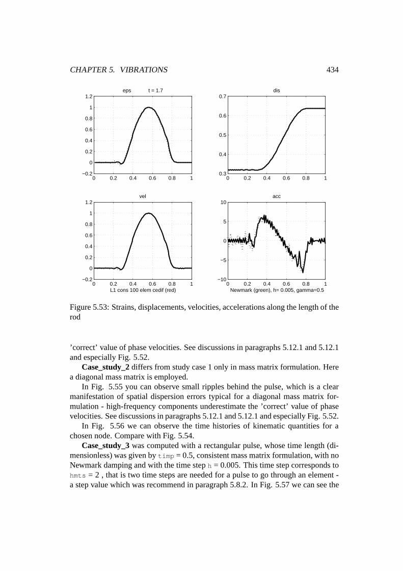
CHAPTER 5. VIBRATIONS 434
0 0.2 0.4 0.6 0.8 1−0.2
0
0.2
0.4
0.6
0.8
1
1.2eps t = 1.7
0 0.2 0.4 0.6 0.8 10.3
0.4
0.5
0.6
0.7dis
0 0.2 0.4 0.6 0.8 1−0.2
0
0.2
0.4
0.6
0.8
1
1.2vel
L1 cons 100 elem cedif (red)0 0.2 0.4 0.6 0.8 1
−10
−5
0
5
10acc
Newmark (green), h= 0.005, gamma=0.5
Figure 5.53: Strains, displacements, velocities, accelerations along the length of therod
’correct’ value of phase velocities. See discussions in paragraphs 5.12.1 and 5.12.1and especially Fig. 5.52.
Case_study_2differs from study case 1 only in mass matrix formulation. Herea diagonal mass matrix is employed.
In Fig. 5.55 you can observe small ripples behind the pulse, which is a clearmanifestation of spatial dispersion errors typical for a diagonal mass matrix for-mulation - high-frequency components underestimate the ’correct’ value of phasevelocities. See discussions in paragraphs 5.12.1 and 5.12.1 and especially Fig. 5.52.
In Fig. 5.56 we can observe the time histories of kinematic quantities for achosen node. Compare with Fig. 5.54.
Case_study_3was computed with a rectangular pulse, whose time length (di-mensionless) was given bytimp = 0.5, consistent mass matrix formulation, with noNewmark damping and with the time steph = 0.005. This time step corresponds tohmts = 2 , that is two time steps are needed for a pulse to go through an element -a step value which was recommend in paragraph 5.8.2. In Fig. 5.57 we can see the

CHAPTER 5. VIBRATIONS 435
0 50 100 150 200 250 300 3500
0.1
0.2
0.3
0.4
history of displacement (in time steps)
node = 33 L1 cons 100 elem cedif (red) Newmark (green), h= 0.005, gamma=0.5
0 50 100 150 200 250 300 350−0.5
0
0.5
1
1.5
history of velocity (in time steps)
0 50 100 150 200 250 300 350−10
−5
0
5
10
history of acceleration (in time steps)
Figure 5.54: Histories of kinematic quantities at a chosen node
distribution of kinematic quantities along the length of the rod.Here we can clearly see that dealing with discontinuities is not easy. While the
displacement distribution is more than acceptable, the distribution of strains andvelocities contain the unwanted high-frequency components of the discontinuouspulse (see Fig. 5.13) magnified by space and time dispersion effects. Accelerationdata - as computed by finite element method in this case - are almost pure garbage,they are completely worthless. One should realize, however, that what we are de-manding of finite element computation is impossible to achieve.
Look at the displacement distribution in Fig. 5.58 - it is a continuous function oftime coordinate having two changes in its tangent. Velocity, as the first derivative ofdisplacements with respect to time, should have two sudden jumps - discontinuities- of finite lengths at these locations. And acceleration - as the time derivative ofvelocity - should have two peaks of infinite lengths (Dirac functions) there. This isreally beyond the capabilities of any discrete method.
There is another fact that should be kept in mind, namely the impossibility ofphysical realization of a purely rectangular or Heaviside pulses. Still, using these

CHAPTER 5. VIBRATIONS 436
0 0.2 0.4 0.6 0.8 1−0.2
0
0.2
0.4
0.6
0.8
1
1.2eps t = 1.7
0 0.2 0.4 0.6 0.8 10.3
0.4
0.5
0.6
0.7dis
0 0.2 0.4 0.6 0.8 1−0.2
0
0.2
0.4
0.6
0.8
1
1.2vel
L1 diag 100 elem cedif (red)0 0.2 0.4 0.6 0.8 1
−10
−5
0
5
10acc
Newmark (green), h= 0.005, gamma=0.5
Figure 5.55: Strains, displacements, velocities, accelerations along the length of therod
pulses for testing the finite element method and the methods of integration is quiteexpedient since this is really the worst case scenario telling us that whatever wewould tackle in the real world would always be better.
Sometimes, the high frequency components are numerically filtered out by thenumerical or real damping which is introduced into the computation; however, thisis always at the expense of the violation of the energy conservation in the mechani-cal system. One way to introduce the numerical damping into the computation is tovary the Newmarkgammaparameter as it is shown in the following text.
Case_study_4differs from the previous one only by the value of thegamma
parameter which is set to 0.7 here and was 0.5 in study_case_3.Observe carefully Fig. 5.59 and 5.60 and compare them with Fig. 5.57 and
5.58. You should notice that the distributions computed by the central differencemethod are the same as before. The results computed by Newmark are smoother,however, and are really appealing to engineering eyes. Notice that the history ofaccelerations, depicted in Fig. 5.60, correctly indicates both peaks corresponding

CHAPTER 5. VIBRATIONS 437
0 50 100 150 200 250 300 3500
0.1
0.2
0.3
0.4
history of displacement (in time steps)
node = 33 L1 diag 100 elem cedif (red) Newmark (green), h= 0.005, gamma=0.5
0 50 100 150 200 250 300 350−0.5
0
0.5
1
1.5
history of velocity (in time steps)
0 50 100 150 200 250 300 350−10
−5
0
5
10
history of acceleration (in time steps)
Figure 5.56: Histories of kinematic quantities at a chosen node
to the wave fronts of the pulse. Since there is no such thing as a free lunch we haveto pay for the smoothness somehow. One penalty which is clearly observable isthat the wave fronts are less steep, another - not seen at the first sight - is that theNewmark method forgamma> 0:5 does not conserve energy. See paragraph 5.8.2.
Case_study_5differs from the study_case_3 only in the time step value that isset h = 0.001 here and was five times greater before. This means that ten time stepsare needed for a wave front to pass through the length of one element, sohmts =10 in this case. This is a very small time step, usually we cannot afford such whensolving practical engineering tasks.
Observing the results presented in Fig. 5.61 and 5.62 we disappointedly con-clude that the results are not ’better’ even if they were obtained in a more costlyway with the time step five times smaller than that in the study_case_3.
In this case the usual disretization rule of thumb - the smaller the better - doesnot hold. Using too small time step results in more precise integration of those high-frequency components of the loading pulse spectrum that are wrong due to spatialdispersion effects. On the other hand we clearly see that the Newmark and the cen-

CHAPTER 5. VIBRATIONS 438
0 0.2 0.4 0.6 0.8 1−1
−0.5
0
0.5
1
1.5eps t = 1.7
0 0.2 0.4 0.6 0.8 10.4
0.5
0.6
0.7
0.8
0.9
1
1.1dis
0 0.2 0.4 0.6 0.8 1−0.5
0
0.5
1
1.5vel
L1 cons 100 elem cedif (red)0 0.2 0.4 0.6 0.8 1
−100
−50
0
50
100acc
Newmark (green), h= 0.005, gamma=0.5
Figure 5.57: Strains, displacements, velocities, accelerations along the length of therod
tral difference results are becoming closer since using a small time step minimizesthe errors due to temporal dispersion.
Case_study_6has the same small time step as the case_study_5 but the diagonalmass matrix formulation was used for the computation. The results are presentedin Fig. 5.63 and 5.64. Again, we can observe the spurious side effect of oscilla-tions behind the pulse appearing due to FE underestimation of the phase velocityof high-frequency components of the loading pulse - in contradistinction to resultspresented in case_study_5 where the consistent mass matrix formulation was used.As mentioned earlier in paragraphs 5.12.1 and 5.12.1, the consistent mass matrixoverestimates the phase velocities of high-frequency components and leads to theexistence of spurious oscillations in front of the pulse.
The reader is urged to proceed with changing the input parameters of theVTVbarl1nc.m program to get a clear insight into the numerical processes and theirimpact on the finite element modelling of stress wave propagation.
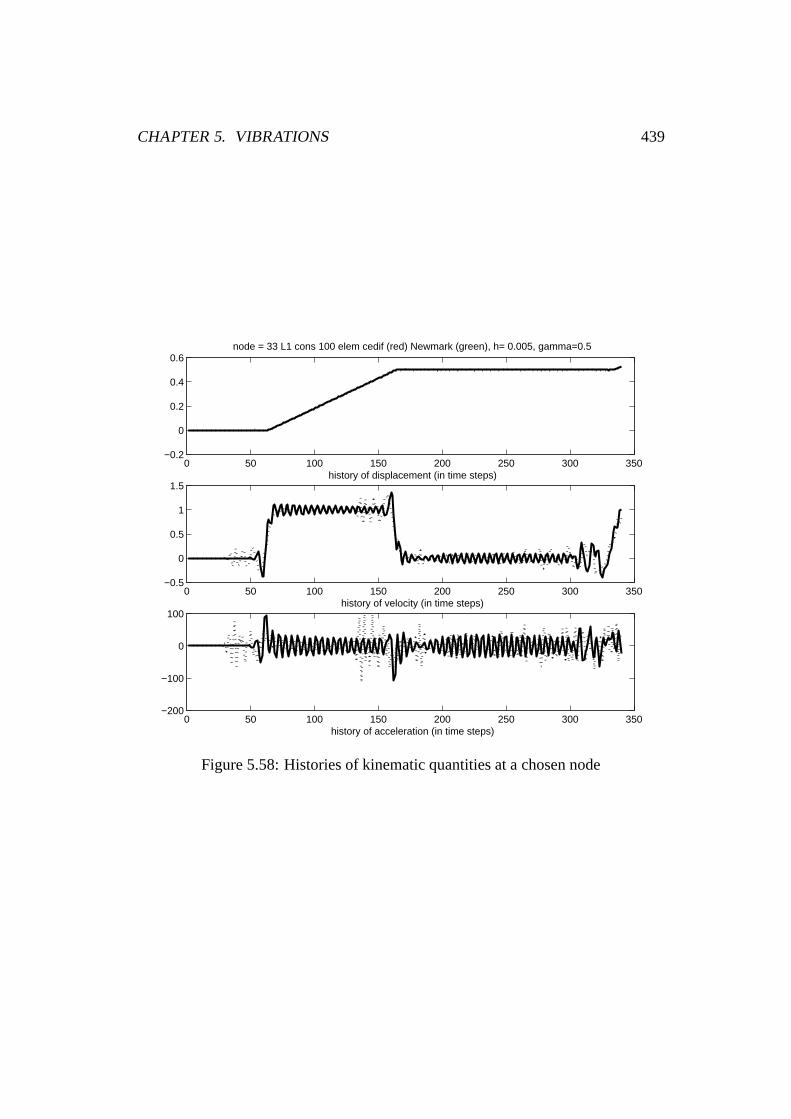
CHAPTER 5. VIBRATIONS 439
0 50 100 150 200 250 300 350−0.2
0
0.2
0.4
0.6
history of displacement (in time steps)
node = 33 L1 cons 100 elem cedif (red) Newmark (green), h= 0.005, gamma=0.5
0 50 100 150 200 250 300 350−0.5
0
0.5
1
1.5
history of velocity (in time steps)
0 50 100 150 200 250 300 350−200
−100
0
100
history of acceleration (in time steps)
Figure 5.58: Histories of kinematic quantities at a chosen node

CHAPTER 5. VIBRATIONS 440
0 0.2 0.4 0.6 0.8 1−1
−0.5
0
0.5
1
1.5eps t = 1.7
0 0.2 0.4 0.6 0.8 10.4
0.5
0.6
0.7
0.8
0.9
1
1.1dis
0 0.2 0.4 0.6 0.8 1−0.5
0
0.5
1
1.5vel
L1 cons 100 elem cedif (red)0 0.2 0.4 0.6 0.8 1
−100
−50
0
50
100acc
Newmark (green), h= 0.005, gamma=0.7
Figure 5.59: Strains, displacements, velocities, accelerations along the length of therod

CHAPTER 5. VIBRATIONS 441
0 50 100 150 200 250 300 350−0.2
0
0.2
0.4
0.6
history of displacement (in time steps)
node = 33 L1 cons 100 elem cedif (red) Newmark (green), h= 0.005, gamma=0.7
0 50 100 150 200 250 300 350−0.5
0
0.5
1
1.5
history of velocity (in time steps)
0 50 100 150 200 250 300 350−200
−100
0
100
history of acceleration (in time steps)
Figure 5.60: Histories of kinematic quantities at a chosen node

CHAPTER 5. VIBRATIONS 442
0 0.2 0.4 0.6 0.8 1−0.5
0
0.5
1
1.5eps t = 1.7
0 0.2 0.4 0.6 0.8 10.4
0.5
0.6
0.7
0.8
0.9
1
1.1dis
0 0.2 0.4 0.6 0.8 1−0.5
0
0.5
1
1.5vel
L1 cons 100 elem cedif (red)0 0.2 0.4 0.6 0.8 1
−100
−50
0
50
100acc
Newmark (green), h= 0.001, gamma=0.5
Figure 5.61: Strains, displacements, velocities, accelerations along the length of therod

CHAPTER 5. VIBRATIONS 443
0 200 400 600 800 1000 1200 1400 1600 1800−0.2
0
0.2
0.4
0.6
history of displacement (in time steps)
node = 33 L1 cons 100 elem cedif (red) Newmark (green), h= 0.001, gamma=0.5
0 200 400 600 800 1000 1200 1400 1600 1800−0.5
0
0.5
1
1.5
history of velocity (in time steps)
0 200 400 600 800 1000 1200 1400 1600 1800−100
−50
0
50
100
history of acceleration (in time steps)
Figure 5.62: Histories of kinematic quantities at a chosen node

CHAPTER 5. VIBRATIONS 444
0 0.2 0.4 0.6 0.8 1−0.5
0
0.5
1
1.5eps t = 1.7
0 0.2 0.4 0.6 0.8 10.4
0.5
0.6
0.7
0.8
0.9
1
1.1dis
0 0.2 0.4 0.6 0.8 1−0.5
0
0.5
1
1.5vel
L1 diag 100 elem cedif (red)0 0.2 0.4 0.6 0.8 1
−30
−20
−10
0
10
20
30
40acc
Newmark (green), h= 0.001, gamma=0.5
Figure 5.63: Strains, displacements, velocities, accelerations along the length of therod

CHAPTER 5. VIBRATIONS 445
0 200 400 600 800 1000 1200 1400 1600 18000
0.2
0.4
0.6
0.8
history of displacement (in time steps)
node = 33 L1 diag 100 elem cedif (red) Newmark (green), h= 0.001, gamma=0.5
0 200 400 600 800 1000 1200 1400 1600 1800−0.5
0
0.5
1
1.5
history of velocity (in time steps)
0 200 400 600 800 1000 1200 1400 1600 1800−50
0
50
history of acceleration (in time steps)
Figure 5.64: Histories of kinematic quantities at a chosen node

CHAPTER 5. VIBRATIONS 446
Vibrations of a planar truss structure - finite element approach
0 5 10 15 20 250
5
10
15
20
25Truss structure
truss plot.m
Dimensions are in [m]
Figure 5.65: A sketch of a planar structure - dimensions
Let’s find natural frequencies and corresponding modes of vibration of a sim-plified two-dimensional truss structure whose dimensions and shape are sketched inFig.5.65. The finite element method is to be employed. We assume that the trussesare connected by frictionless joints. From this modelling assumption, it follows thattruss elements are loaded by axial forces only - no bending can occur. The structureis constrained by means of the lowest two joints that are fixed but, in these as inothers, the rotational degrees of freedom are allowed. The geometrical propertiesof the structure are as follows

CHAPTER 5. VIBRATIONS 447
length [m] cross-sectional area [m2]Vertical trusses 7.5 8:10�5
Horizontal trusses 5 6:10�5
Diagonal trussesp7:52 + 52 4:10�5
The material of all the truss elements of the structure is assumed to be the sameand is characterized by Young’s modulusE = 7:17 1010 Nm�2 and the density� = 2768 kgm�3.
1D-truss elements could be utilized for the solution of this problem. In the localcoordinate system, one of whose coordinate axis is identical with the longitudinalcenterline of the truss, the mass and stiffness matrices (see paragraph 5.12.1 andnumerous finite element references as [6], [1]) are
�m =�A l
6
�2 11 2
�and �k =
E A
l
�1 �1�1 1
�: (5.312)
In Eq. (5.312) the variable� denotes the density,A is the cross sectional area,lis the length andE is the Young’s modulus. To employ this element in 2D space, wehave to add additional local degrees of freedom - perpendicular to the truss’s longi-tudinal axis. In the case of a stiffness matrix they are purely fictitious, neverthelessin case of a mass matrix they are quite real. See [6] for details. Their alternativeforms are
�m =�A l
6
26642 0 1 00 2 0 11 0 2 00 1 0 2
3775 and �k =
EA
l
2664
1 0 �1 00 0 0 0�1 0 1 00 0 0 0
3775 : (5.313)
Now, it is necessary to transform the matrices, expressed in their respective localcoordinate systems (denoted by a bar), into a coordinate system, which is uniquefor all the elements. Such a system is usually called the global coordinate system.
Let’s recall the orthogonal transformation of coordinates between two coordi-nate systems depicted in Fig. 5.66.
The element displacements in a local coordinate system are denoted by�q , thelocal displacements in a global coordinate system byq. Similarly, the elementforces are denoted�P andP respectively.
By inspecting the relations between local and global displacements appearingin Fig. 5.66, we can write the following matrix equation
q = R�q; (5.314)
which, written in full, reads8>><>>:
q1q2q3q4
9>>=>>; =
2664cos� � sin� 0 0sin� cos� 0 00 0 cos� � sin�0 0 sin� cos�
37758>><>>:
�q1�q2�q3�q4
9>>=>>; : (5.315)

CHAPTER 5. VIBRATIONS 448
q1
q1 α
q3
q4
q2
x
x
y
y
q2
q3
q4
Figure 5.66: Transformation of orthogonal coordinate system
Due to orthogonality conditions the inverse transformation simplifies to
�q = R�1q = RTq = Tq; (5.316)
where we have introduced a new matrixT, being the transpose ofR, in the form
T =
2664
cos� sin� 0 0� sin� cos� 0 0
0 0 cos� sin�0 0 � sin� cos�
3775 : (5.317)
Surely, the conditions of equilibrium have to be independent of the choice ofcoordinate system, so they should hold both in local
�P = �k�q; (5.318)
and as well as in globalP = kq (5.319)
coordinate systems.Substituting the transformation (5.316) for displacements and forces into Eq.
(5.318) and rearranging the formula slightly, we get
P = TT�kTq: (5.320)
Comparing Eq. (5.320) with (5.319) we come to
k = TT�kT; (5.321)
CHAPTER 5. VIBRATIONS 449
that is the desired equation expressing the stiffness matrix in the global coordi-nate system in terms of its elements from the local coordinate system. Evaluatingtrigonometric functions in Eq. (5.321) analytically we could get an equivalent rela-tion for the stiffness matrix. The programVTStest3.m , listed below, gives
k = E*A/l [ c^2, c*s, -c^2, -c*s][ c*s, s^2, -c*s, -s^2][-c^2, -c*s, c^2, c*s][-c*s, -s^2, c*s, s^2].
Reading the programVTStest3.m reveals that a brief notation forc = cos� ands = sin� was introduced.
A similar reasoning leads to mass matrix transformation in the form
m = TT �mT: (5.322)
Carrying out the multiplication in (5.322) analytically (seeVTStest3.m again)we get
m = A*ro*l/6*[2*c^2+2*s^2, 0,2*c^2+2*s^2, 0][ 0,2*c^2+2*s^2, 0, c^2+s^2][ c^2+s^2, 0,2*c^2+2*s^2, 0][ 0, c^2+s^2, 0,2*c^2+2*s^2],
which proves that the matricesm and �m are identical so the transformation(5.322) need not be carried out. The programVTStest3.m is as follows.
% VTStest3% stiffness and mass matrices of a truss element% are expressed in local and global coordinate systems% multiplicative constants are left outclear; format compactsyms t tt c s % declare symbolic variables% transformation matrix and its transposet = [c s 0 0; -s c 0 0; 0 0 c s; 0 0 -s c];tt= [c -s 0 0; s c 0 0; 0 0 c -s; 0 0 s c];% stiffness matrix in local coordinateskb = [1 0 -1 0; 0 0 0 0; -1 0 1 0; 0 0 0 0];% consistent and diagonal mass matrices in local coordinatesmcb = [2 0 1 0; 0 2 0 1; 1 0 2 0; 0 1 0 2];mdb = [3 0 0 0; 0 3 0 0; 0 0 3 0; 0 0 0 3];% all three matrices in global coordinate systemdisp(’multiplicative constants are left out’)disp(’stiffness matrix’)k = tt*kb*tmc = tt*mcb*t;mc1=subs(mc,2*c^2+2*s^2,2);disp(’consistent mass matrix - independent of coordinate ...

CHAPTER 5. VIBRATIONS 450
transformation’)subs(mc1,c^2+s^2,1)md = tt*mdb*t;disp(’diagonal mass matrix - independent of coordinate ...transformation’)subs(md,3*c^2+3*s^2,3)% try to unpercent the following three statements% pretty(k)% latex(k)% fortran(k)% end of VTStest3
The output ofVTStest3.m is as follows.
>>VTStest3multiplicative constants are left outstiffness matrixk =[ c^2, c*s, -c^2, -c*s][ c*s, s^2, -c*s, -s^2][ -c^2, -c*s, c^2, c*s][ -c*s, -s^2, c*s, s^2]consistent mass matrix - independent of coordinate transformationans =
2 0 1 00 2 0 11 0 2 00 1 0 2
diagonal mass matrix - independent of coordinate transformationans =
3 0 0 00 3 0 00 0 3 00 0 0 3
Now, let’s show how the global mass and stiffness matrices for the whole struc-ture are assembled. At first one has to number the nodes, global degrees of freedomand elements. A possible way is depicted in Fig. 5.67.
Accepting the dof’s numbering depicted in Fig. 5.67 we can list the correspond-ing code numbers element-wise from element 1 to 15 into a vector, sayd,
% code numbers of all the elementsd=[ 1 2 3 4; 1 2 5 6; 1 2 7 8; 5 6 3 4; ...
3 4 7 8; 5 6 7 8; 5 6 9 10; 5 6 11 12; ...9 10 7 8; 7 8 11 12; 9 10 11 12; 9 10 13 14; ...9 10 15 16; 13 14 11 12; 11 12 15 16];
Lengths, cross-sectional areas and truss orientations are as follows

CHAPTER 5. VIBRATIONS 451
↑2
→1 ↑4
→3
↑6
→5 ↑8
→7
↑10
→9 ↑12
→11
↑14
→13 ↑16
→15
1
6
11
2 3 4 5
7 8 9 10
12 13 14 15
4 5
3 6
2 7
1 8
Truss structure numberingelements (red)nodes (blue)dofs (black)
stoz plot v
Figure 5.67: Node, element and dof’s numbering

CHAPTER 5. VIBRATIONS 452
% lengths of elements in [m]l=[5 7.5 9.01 9.01 7.5 5 7.5 9.01 9.01 7.5 5 7.5 9.01 9.01 7.5];% cross sections of elements in [m^2]a=[6 8 4 4 8 6 8 4 4 8 6 8 4 4 8]*1e-5;% orientation of trusses with respect of x-axis by angles in radiansb1=pi/2; b2=atan(l(2)/l(1));alf=[0 -b1 -b2 b2 -b1 0 -b1 -b2 b2 -b1 0 -b1 -b2 b2 -b1];
Assembling the global matrices in the finite element method is based on topol-ogy considerations and is described in detail in numerous finite element textbooksas in [6], [1].
It can be shown that the code numbers play the role of pointers, directing theelements of local element matrices to their proper locations in global ones. Toimplement this process efficiently, the Matlab philosophy - allowing an array to beused as a pointer itself - is the best thing we could dream of. If we assume that all theelements are of the same type, the whole assembling process could be programmedas simply as that
% assemble global stiffness and mass matrices
% imax is the global number of degrees of freedom (structure)% kmax is number of elements% lmax is number local degrees of freedom of an element% zeroing of arrayskglobal = zeros(imax,imax);mglobal = zeros(imax,imax);for k=1:kmax % loop over all the elements
kelem = ... get element stiffness matrix of k-th elementmelem = ... get element mass matrix of k-th elementc = ... get code numbers of the k-th element
%size of c is(1,lmax)kglobal(c,c) = kglobal(c,c) + kelem;mglobal(c,c) = mglobal(c,c) + melem;
% note: size of kelem and melem is (lmax,lmax)end;
See also the functionVTSglobv.m for more details.In the case of this particular example the procedures generating the stiffness
and mass matrices (VTSrigbarv.m andVTSmasbarv.m ) could be implemented asfollows
function xke=VTSrigbarv(ey,l,a,alf)% local stiffness matrix of a truss element% with 4 dof’s% ey ... Young modulus% l .... length of element% a .... cross sectional area% alf .. an oriented angle between x-axis and truss (in radians)

CHAPTER 5. VIBRATIONS 453
konst=ey*a/l;kbar4 = [1 0 -1 0; 0 0 0 0; -1 0 1 0; 0 0 0 0];c = cos(alf); s = sin(alf);t = [c s 0 0; -s c 0 0; 0 0 c s; 0 0 -s c];xke = konst*t’*kbar4*t;
% this is an alternative way how to do it% c=cos(alf); s=sin(alf);% k=[1 -1; -1 1];% t=[c s 0 0 ; 0 0 c s];% xke=konst*t’*k*t;% end of VTSrigbarv
function xme=VTSmasbarv(ro,l,a,alf,icons)% xme mass matrix of a 2d truss element% ro density% l length of truss% alf angle measured from global x to truss centreline% icons mass matrix formulation switch% = 1 ... consistent% = 0 ... diagonalif icons == 1,
m = [2 0 1 0; 0 2 0 1; 1 0 2 0; 0 1 0 2];else
m = [3 0 0 0; 0 3 0 0; 0 0 3 0; 0 0 0 3];endkonst=ro*l*a/6;% c=cos(alf); s=sin(alf);% t=[c s 0 0; -s c 0 0; 0 0 c s; 0 0 -s c];% xme=konst*t’*m*t;xme = konst*m;% there is no need to carry out the coordinate transformation% since the mass matrix is insensitive to it
% end of VTSmasbarv
The main program coordinating all the needed activities including implementa-tion of constraints (notice the vectorbound containing the pointers to those dof’sthat are fixed to the frame, i.e. identically equal to zero), eigenvalue computationand plotting of eigenmodes could have the following form
% VTSstozar33w is a matlab program calculating% the eigenvalues and eigenvectors of a truss structure.% main variables% xm, xk, ....... global mass and stiffness matrices% xme,xke ....... local mass and stifness matrices% imax .......... number of generalized displacements% lmax .......... number of local degrees of freedom
CHAPTER 5. VIBRATIONS 454
% kmax .......... number of elements% input valuesclear; d=clock; disp([d(3) d(2) d(1) d(4) d(5)])format short; format compact% input datakmax=15; % number of elementsimax=16; % number of generalized d.o.f.imaxb=4; % number of prescribed zero bound. displ.imaxc=imax-imaxb; % number of condensed d.o.f.% nodal coordinatesx=[10 10 10 10 15 15 15 15];y=[0 7.5 15 22.5 22.5 15 7.5 0];% pointers to x-displacements at nodes
xp=[13 9 5 1 3 7 11 15];% pointers to y-displacements at nodes
yp=[14 10 6 2 4 8 12 16];% plot outline of meshfigure(1)plot(x,y,’o’,x,y); axis([0,25,0,25]); axis(’equal’)% code numbers of all the elementsd=[ 1 2 3 4; 1 2 5 6; 1 2 7 8; 5 6 3 4; ...
3 4 7 8; 5 6 7 8; 5 6 9 10; 5 6 11 12; ...9 10 7 8; 7 8 11 12; 9 10 11 12; 9 10 13 14; ...9 10 15 16; 13 14 11 12; 11 12 15 16];
% bound. conditions - pointers to prescribed zero displacementsbound=[13 14 15 16];% lengths of elements in [m]l=[5 7.5 9.01 9.01 7.5 5 7.5 9.01 9.01 7.5 5 7.5 9.01 9.01 7.5];% cross sections of elements in [m^2]a=[6 8 4 4 8 6 8 4 4 8 6 8 4 4 8]*1e-5;% orientation of trusses with respect of x-axis% by angles in radiansb1=pi/2; b2=atan(l(2)/l(1));alf=[0 -b1 -b2 b2 -b1 0 -b1 -b2 b2 -b1 0 -b1 -b2 b2 -b1];% Young modulus in [N/m^2]ey=7.17e10;% density in [kg/m^3];ro=2768;% assemble stiffness and mass matrices% and choose mass matrix formulationicons = ...input(’1 = consistent, 0 = diagonal, enter 1 or 0 ... ’);if icons == 1,
masslabel = [’consistent mass matrix’]; disp(masslabel);else
masslabel = [’diagonal mass matrix’]; disp(masslabel);end[xk,xm]=VTSglobv(d,kmax,imax,alf,ro,l,a,ey,icons);% make copies

CHAPTER 5. VIBRATIONS 455
xkcopy=xk; xmcopy=xm;% calculate eigenvalues for unconstrained global matricesl2=eig(xk,xm); r2k=rank(xk); r2m=rank(xm);disp(’ ’)disp(’size of full (unconstrained) matrices’)size_xk = size(xk), size_xm = size(xm)disp(’ ’)disp(’rank of unconstrained stiffness and mass matrices’)disp([r2k r2m]);disp(’eigenvalues for unconstrained global matrices’)disp(sort(real(l2’)));% taking the prescribed boundary conditions into account% by deleting rows and columns corresponding to zero dof’s% this process is sometimes called condensing matricesxk(bound,:)=[]; xm(bound,:)=[];xk(:,bound)=[]; xm(:,bound)=[];l=eig(xk,xm);disp(’ ’)disp(’size of condensed matrices’)size_xk_cond = size(xk), size_xm_cond = size(xm)disp(’ ’)disp(’rank of condensed stiffness and mass matrices’)rk=rank(xk); rm=rank(xm); disp([rk rm])disp(’eigenvalues by condensed matrices’)disp(sort(l’))% there is another way how to do it, i.e.% penalty approach - just for checking purposes% instead of deleting rows and columns large numbers% are put into corresponding diagonal positionsfor i=1:4
xkcopy(bound(i),bound(i))=1e10;xmcopy(bound(i),bound(i))=1e10;
endl1=eig(xkcopy,xmcopy); r1k=rank(xk); r1m=rank(xm);disp(’ ’)disp(’size of penalty treated matrices’)size_xk_penalty = size(xkcopy), size_xm_penalty = size(xmcopy)disp(’ ’)disp(’rank of stiffness and mass matrices - penalty’);disp([r1k r1m])disp(’eigenvalues by penalty approach’);disp(sort(l1’))format long el=sort(eig(xk,xm)); om=sqrt(l); f=om/(2*pi);disp(’sorted eigenvalues, angular frequencies and frequencies’)[l om f][v ll]=eig(xk,xm);[sorted_eigenvalues,order] = sort(diag(ll));sorted_ang_frequencies = sqrt(sorted_eigenvalues);

CHAPTER 5. VIBRATIONS 456
sorted_freq_in_Hz = sorted_ang_frequencies/(2*pi);
figure(2)% plot all eigenvectors
coefx=2; coefy=2;for i=1:imaxc
subplot(3,4,i)dd=v(:,order(i));ddf=[dd’ 0 0 0 0];ddx=ddf(xp); ddy=ddf(yp);xdef=x+coefx*ddx; ydef=y+coefy*ddy;plot(x,y,’o’, x,y, xdef,ydef,’x’, xdef,ydef,’r’);axis(’equal’);title(num2str(sorted_freq_in_Hz(i))); axis off
endtext(1,-5,masslabel);string_icons = int2str(icons);file_name = [’VTSstozar33w’ string_icons];print(’-dmeta’, file_name)print(’-deps’, file_name)% end of VTSstozar33w
The printed output fromVTSstozar33w.m is presented here with authors’ com-ments. They are printed in Italics to be easily distinguishable from the programoutput which is in Courier.
VTSstozar33w
When started, the program prints the current date and time in dd mm yy hr mnformat.12 7 2000 15 40
Then it asks the user to choose the mass formulation to be employed.1 = consistent, 0 = diagonal, enter 1 or 0 please ... 0
Diagonal mass matrix was chosen here, the program prompt isdiagonal mass matrix
Size of assembled global matrices is computed. Both mass and stiffness matrix are16 by 16, since we have 16 degrees of freedom corresponding to 8 nodes, eachhaving 2 independent displacements defined.size of full (unconstrained) matrices
size_xk =
16 16
sizei_xm =
16 16
So far no boundary conditions were prescribed. Physically the considered structureis not constrained which means that it is not attached to the fixed frame and it canfreely move - as a body in 2D space has 3 rigid body degrees of freedom. Thenulity of the global stiffness is 3, corresponding thus to three rigid body degrees of

CHAPTER 5. VIBRATIONS 457
freedom. Such a matrix is singular and its rank = size - nulity = 13. Notice that themass matrix is regular, its rank equals the size.rank of unconstrained stiffness and mass matrices
13 16
There are 16 eigenvalues of the generalized eigenvalue problem, three of thembeing equal to zero since the structure has 3 rigid body modes. They are sorted inascending order. Those are not, however, the natural frequencies we are interestedin.eigenvalues for unconstrained global matrices
1.0e+006 *
Columns 1 through 7
-0.0000 -0.0000 0.0000 0.0467 0.0537 0.1020 0.3019
Columns 8 through 14
0.3302 0.5133 0.5744 0.6718 0.8303 0.9196 1.0228
Columns 15 through 16
1.1041 1.3260
Assembled global matrices should be aware of the prescribed boundary conditions(constraints). In our case there are four dof ’s displacements that are identicallyequal to zero (at nodes 1 and 10, the displacements 13, 14, 15 and 16). Since thesedisplacements are equal to zero, they do not contribute to the solution and thecorresponding rows and columns could be deleted from the assembled matrices.This way - by condensation - the problem is regularized. Notice that the rank ofstiffness and mass matrices equals their size.size of condensed matrices
size_xk_cond =
12 12
size_xm_cond =
12 12
rank of condensed stiffness and mass matrices
12 12
For the constrained structure there are 12 non-zero eigenvalues corresponding to12 by 12 global mass and stiffness matrices. Those are the eigenvalues we arelooking for.eigenvalues by condensed matrices
1.0e+006 *
Columns 1 through 7
0.0025 0.0310 0.0795 0.0971 0.3557 0.5348 0.6233
Columns 8 through 12
0.6285 0.6892 0.9157 1.0032 1.2066
There is an alternative treatment by a so-called penalty method. Instead of deletingthe rows and columns corresponding to zero degrees of freedom we are adding

CHAPTER 5. VIBRATIONS 458
’big’ numbers to the corresponding diagonal terms in assembled matrices. Wecould imagine that instead of prescribing zero displacements at constrained nodes,we add four very stiff linear springs there. So instead of exact zero displacementswe get displacements at constrained nodes that are very small as compared toothers. Notice that the size of matrices is not changed, which is computationallyadvantageous when dealing with large matrices. Now, the rank of assembledmatrices is 16, they are regular, however.size of penalty treated matrices
size_xk_penalty =
16 16
size_xm_penalty =
16 16
rank of stiffness and mass matrices - penalty
16 16
There are four very small eigenvalues, close to zero, the remaining 12 have almostthe same values as those obtained by ’condensation’. This approach is slightlyless precise than the previous one - check that the relative error of 12 ’nonzero’eigenvalues is negligible and quite sufficient for engineering purposes.eigenvalues by penalty approach
1.0e+006 *
Columns 1 through 7
0.0000 0.0000 0.0000 0.0000 0.0025 0.0310 0.0795
Columns 8 through 14
0.0971 0.3557 0.5348 0.6233 0.6285 0.6892 0.9157
Columns 15 through 16
1.0032 1.2066
Here, at last, are the results. It should be reminded that angular frequencies[radi-ans/s]are square roots of eigenvalues and frequencies[1/s] are eigenfrequenciesdivided by 2*pisorted eigenvalues, angular frequencies and frequencies
ans =
2.516009837282328e+003 5.015984287537520e+001
7.983186938328752e+000
3.095373356961773e+004 1.759367317237015e+002
2.800120052525978e+001
7.952337879468736e+004 2.819988985699898e+002
4.488151865388389e+001
9.706814361482544e+004 3.115576088219086e+002
4.958593350189786e+001
3.557304914052800e+005 5.964314641308589e+002
9.492501573196266e+001

CHAPTER 5. VIBRATIONS 459
5.347833973383781e+005 7.312888603953832e+002
1.163882369599642e+002
6.233326480383119e+005 7.895141848240043e+002
1.256550851559085e+002
6.284790716006934e+005 7.927667195339959e+002
1.261727421325817e+002
6.892363560497927e+005 8.302025993995638e+002
1.321308474621812e+002
9.157385277948167e+005 9.569422802838302e+002
1.523020941608015e+002
1.003235617872196e+006 1.001616502396100e+003
1.594122174387545e+002
1.206583162662665e+006 1.098445794139458e+003
1.748230778557973e+002
End of comments and VTSstozar33w.m output for a diagonal mass matrixformulation.
Natural frequencies expressed in [Hz] and the corresponding modes of vibrationcomputed with a consistent mass matrix formulation are shown in Fig. 5.68 whilethose computed with a diagonal mass matrix formulation are in Fig. 5.69.
It should be noticed that frequencies for mass matrix formulation are higherthan those computed with a diagonal one. This is due to the dispersive propertiesof linear strain elements (see in paragraph 5.12.1 ). One could conclude that the’actual’ values of frequencies are bounded by those computed with consistent anddiagonal formulations. Also, one should realize that only the lower part of thespectrum computed by finite elements is reliable.
Notice the modes of vibration associated with natural frequencies. On the lowerpart of the spectrum we have a bending mode, corresponding to the fact that thestructure is least stiff or the most flexible in this respect. Buckling modes cor-responding to the stiffest behaviour of the structure are on the other side of thespectrum

CHAPTER 5. VIBRATIONS 460
8.2285 33.0512 45.7661 69.9307
116.3646 140.7633 159.2753 162.1971
164.1558 204.8688 210.2205 248.2669
consistent mass matrix
Figure 5.68: Natural frequencies [Hz] and corresponding modes of vibration for aconsistent mass matrix

CHAPTER 5. VIBRATIONS 461
7.9832 28.0012 44.8815 49.5859
94.925 116.3882 125.6551 126.1727
132.1308 152.3021 159.4122 174.8231
diagonal mass matrix
Figure 5.69: Natural frequencies [Hz] and corresponding modes of vibration for adiagonal mass matrix

CHAPTER 5. VIBRATIONS 462
5.12.2 Beams
Free transverse vibration of a thin elastic beam (Bernoulli-Euler theory)
The equation of motion of a long thin beam considered as continuum undergoingtransverse vibration is derived under Bernoulli-Euler assumptions, namely
� there is an axis, say x, of the beam that undergoes no extension,
� the x-axis is located along the neutral axis (i.e unextendable longitudinal axis)of the beam,
� cross sections perpendicular to the neutral axis remain plane during the de-formation - transverse shear deformation is neglected,
� material is linearly elastic and homogeneous,
� the y-axis (one of the principal axes of the cross-section), perpendicular to thex-axis, together with x-axis form a principal plane of the beam.
These assumptions are acceptable for thin beams - the model ignores shear de-formations of a beam element and rotary inertia forces. For more details (see [7] or[5]).
The equation is usually presented in the form
@2
@x2
�EI
@2v
@x2
�+ �A
@2v
@t2= p (x; t) (5.323)
wherex is a longitudinal coordinate,v is a transversal displacement of the beam iny direction, which is perpendicular tox, t is time,E is the Young’s modulus,I isthe planar moment of inertia of the cross section,A is the cross sectional area and� is the density. On the right hand side of the equation there is the loadingp (x; t) -generally a function of space and time - acting in thexy plane.
For free transverse vibrations we have zero on the right-hand side of Eq. (5.323).If bending stiffnessEI is independent of time and space coordinates we can write
@4v
@x4+�A
EI
@2v
@t2= 0: (5.324)
Assuming the steady state vibration in a harmonic form
v(x; t) = V (x) cos(!t� ') (5.325)
and inserting it with its time and space derivatives into Eq. (5.324) we get
d4V (x)
dx4� �4V (x) = 0 (5.326)

CHAPTER 5. VIBRATIONS 463
where we have introduced an auxiliary variable
�4 = �A!2=(EI): (5.327)
The general solution of Eq. (5.326) can be assumed (see [15]) in the form
V (x) = C1 sin h �x + C2 cos h �x + C3 sin�x+ C4 cos�x (5.328)
where constantsC1 toC4 depend on boundary conditions.Example - determine the natural frequencies of a thin cantilever beamLet’s assume that the beam is clamped on its left-hand side where we have put
the origin of coordinate system and sox = 0 there. If the length of the beam isLthen its right-end side coordinate isx = L .
Boundary conditions at the clamped end require that the displacement and itsfirst derivative with respect to spatial coordinate are equal to zero, i.e.
V (x) = 0; (5.329)
dV (x)
dxjx=0 = 0: (5.330)
At the free end of the beam the bending momentM(x) and shear forceT (x) areequal to zero. Let’s recall that the moment is proportional to the second derivative ofthe displacement (curvature) and the shear force is proportional to the first derivativeof the moment with respect to space. So the boundary conditions are
M(L) = EId2V (x)
dx2jx=L = 0; (5.331)
T (L) = EId3V (x)
dx3jx=L = 0: (5.332)
The programVCRchar_eq_beam.m computes the derivatives of the assumed so-lution Eq. (5.328) with respect the to spatial coordinate, substitutes the boundaryconditions values into Eq. (5.329) to (5.332), forms the homogeneous system offour equations with unknownsC1 to C4 and determines the system matrix in theform
[0 1 0 1 ][lam 0 lam 0 ][sinh(lam*L)*lam^2 cosh(lam*L)*lam^2 -sin(lam*L)*lam^2 -cos(lam*L)*lam^2][cosh(lam*L)*lam^3 sinh(lam*L)*lam^3 -cos(lam*L)*lam^3 sin(lam*L)*lam^3]
It is obvious thatlam stands for�. It is known that a homogeneous system ofequations has a non-trivial solution only if its determinant is equal to zero. So theprogram computes the determinant of the above matrix that, after simplificationsdone by the program itself, appears in the form

CHAPTER 5. VIBRATIONS 464
1+cosh(lam*L)*cos(lam*L).
So the frequency equation for a thin cantilever beam is
cosh�L cos �L+ 1 = 0: (5.333)
The frequency equation was obtained by the programVCRfreq_eq_beam_1.m .Read it carefully.
% VCRchar\_eq\_beam_1.m%this program creates and symbolically evaluates%frequency determinant for a free vibration%of a cantilever beam%producing the characteristic equationclearsyms lam x C1 C2 C3 C4 L FD; % define symbolic variables% general solution for Bernoulli-Euler beam isV = ...C1*sinh(lam*x)+C2*cosh(lam*x)+C3*sin(lam*x)+C4*cos(lam*x);% its derivatives areV1 = diff(V,x); V2 = diff(V1,x); V3 = diff(V2,x);
% boundary conditions for the clamped endV0 = subs(V,x,0)V10 = subs(V1,x,0)
%boundary conditions for the free endV2L = subs(V2,x,L)V3L = subs(V3,x,L)
% exctract coefficients by C1, C2, C3, C4% and store them in FD matrixFD(1,1)=subs(V0,{C2,C4},{0,0});FD(1,2)=subs(V0,{C2,C4},{1,0});FD(1,3)=subs(V0,{C2,C4},{0,0});FD(1,4)=subs(V0,{C2,C4},{0,1});
FD(2,1)=subs(V10,{C1,C2,C3,C4},{1,0,0,0});FD(2,2)=subs(V10,{C1,C2,C3,C4},{0,1,0,0});FD(2,3)=subs(V10,{C1,C2,C3,C4},{0,0,1,0});FD(2,4)=subs(V10,{C1,C2,C3,C4},{0,0,0,1});
FD(3,1)=subs(V2L,{C1,C2,C3,C4},{1,0,0,0});FD(3,2)=subs(V2L,{C1,C2,C3,C4},{0,1,0,0});FD(3,3)=subs(V2L,{C1,C2,C3,C4},{0,0,1,0});FD(3,4)=subs(V2L,{C1,C2,C3,C4},{0,0,0,1});
FD(4,1)=subs(V3L,{C1,C2,C3,C4},{1,0,0,0});FD(4,2)=subs(V3L,{C1,C2,C3,C4},{0,1,0,0});FD(4,3)=subs(V3L,{C1,C2,C3,C4},{0,0,1,0});

CHAPTER 5. VIBRATIONS 465
FD(4,4)=subs(V3L,{C1,C2,C3,C4},{0,0,0,1});
FD % print FD matrixfreq_det = det(FD) % compute its determinant
% make simplifications based on the fact% that the determinant is equal zerofreq_det = collect(freq_det,lam^6);freq_det = freq_det/lam^6;freq_det = simplify(freq_det);freq_det = freq_det/2;disp(’frequency determinant is ’)disp([freq_det])% end of VCRchar_eq_beam_1
To determine natural frequencies of a cantilever beam we have to compute theroots of the frequency equation (5.333). Since it is a transcendental equation, anumerical approach using a Matlab build-in functionfzero would be expedient.Analysing the frequency equation by plotting it (do it yourself)
xx = 1:xmax;for xbar = xx
y(xbar) = cos(xbar)*cosh(xbar)+1;endfigure(1)plot(xx,y);% this plot is not in the text - do it yourself
we could observe that the roots are simple (of the first order), and that the func-tional values increasing rapidly with the increasing value of argument due to thecosine hyperbolic function. So the function crosses the x-axis almost perpendicu-larly, which makes the root computation numerically demanding. Since the rootscorrespond to natural frequencies of a system that has no rigid body modes, then allof them are positive and we are interested in positive roots only.
We could compute the roots of the frequency equation by brute force - letting theindependent variable increase in a loop with a constant increment (which must beless than the distance between roots), repeating thus inefficiently the computationof several roots. But as a gift we have we get a simple procedure implemented inthe programVCRroots.m . The procedureVCRf.m defines the frequency equation.In the program we introduced a new variable�x=�L .
% VCRroots% computes a few first roots of the frequency equation% for a thin cantilever beam - analytical approachclear; format long e; format compact;xmax = 30;for xbar = 1:xmax

CHAPTER 5. VIBRATIONS 466
% compute a root in the vicinity of xbarr(xbar) = fzero(’VCRf’,xbar);
end% r % print it if you wish% delete the repeating rootsj = 1; % non-repeated root counterrr(j) = r(j); eps = 1e-10;for xbar=1:xmax-1
if abs(r(xbar+1)-r(xbar))>eps, j=j+1; rr(j)=r(xbar+1); endendrr’% end of VCRroots
function y=VCRf(x)% frequency equation for a thin cantilever beam
y = cos(x)*cosh(x)+1;% end of VCRf
The first ten roots of the frequency equation (5.333), computed by the programVCRroots.m , that are expressed by means of an auxiliary variable
�xi = �iL; (5.334)
are as follows
1 1.875104068711961e+0002 4.694091132974174e+0003 7.854757438237613e+0004 1.099554073487547e+0015 1.413716839104647e+0016 1.727875953208824e+0017 2.042035225104125e+0018 2.356194490180645e+0019 2.670353755551830e+00110 2.984513020910282e+001
To recalculate the�xi - values into natural frequencies, the relations (5.327) and(5.334) should be used leading to
!i =�xiL2
rI
A
sE
�i = 1; 2; 3; : : : (5.335)
One should realize that - even if only ten roots were presented here - the can-tilever beam, considered as continuum, has an infinite number of natural frequen-cies - this is a fact typical for continuous systems described by partial differentialequations.

CHAPTER 5. VIBRATIONS 467
Free transverse vibration of a thin elastic beam (FE - approach)
Example - determine the natural frequencies of a thin cantilever beam using the fi-nite element method. Compare the results with those obtained analytically, treatingthe beam as a continuous system, in paragraph 5.12.2.
A cantilever beam is sketched in Fig. 5.70. Its left end is free, while the rightone if clamped. The length of the beam isL = 1m. Assuming a rectangular crosssectional area with the thicknessb = 0:01 m and the heighth = 0:1 m, we havethe cross sectionA = bh and the planar moment of inertia of the cross sectionI = bh3=12. The Young’s modulus isE = 2:1 1011 N=m2 and the density is� = 7800 kg=m3. The number of elements is set to 10, initially.
kmax
321
L
Figure 5.70: A cantilever beam discretized by beam elements
For the computation we will employ a four-degree-of-freedom beam elementdepicted with numbering of its local degrees of freedom in Fig. 5.71. When mod-elling the beam we will assume that all the elements are of the same geometry andmaterial properties.
4
3
2
1
l0
A,EI,ρ
Figure 5.71: Planar beam element with four degrees of freedom
Generalized displacements numbered 1 and 3 are transversal displacements ofthe beam element, those numbered 2 and 4 are rotations of the deflection curve. Thelength of the element isl.

CHAPTER 5. VIBRATIONS 468
The mass and stiffness matrices of the element are derived in numerous finiteelement references as in ([1], [6], [23]). This element corresponds to Bernoulli-Euler theory for thin beams and thus cannot be subjected to an axial force. Theconsistent mass matrix and the stiffness matrix are as follows.
m =�lA
420
2664
156 22l 54 �13l4l2 13l �3l2
156 �22l2sym: 4l2
3775 ; (5.336)
k =2EI
l3
2664
6 3l �6 3l2l2 �3l l2
6 �3lsym: 2l2
3775 : (5.337)
The Matlab form of the mass and stiffness matrices could have the followingappearance
function [xme]=VBEmasbeam(ro,l1,A);% assemble local mass matrix of a beam% element with 4 dof’s% ro ... density% l1 ... element’s lenght% A .... cross sectional areaxme=zeros(4);l12=l1*l1;konst=ro*l1*A/420;xme(1,1)=156; xme(1,2)=22*l1; xme(1,3)=54; xme(1,4)=-13*l1;
xme(2,2)=4*l12; xme(2,3)=13*l1; xme(2,4)=-3*l12;xme(3,3)=156; xme(3,4)=-22*l1;
xme(4,4)= 4*l12;% symmetryfor i=1:4,
for j=i:4,xme(j,i)=xme(i,j);
end;end;% constant multiplicationxme=konst*xme;% end of VBEmasbeam.m
function [xke]=VBErigbeam(ey,l1,jp);% assemble a local stiffness matrix% of a beam element with 4 dof’s% ey ... Young’s modulus% l1 ... element’s length% jp ... planar moment of inertia of the cross sectionxke=zeros(4);

CHAPTER 5. VIBRATIONS 469
l12=l1*l1; l13=l12*l1;konst=2*ey*jp/l13;xke(1,1)=6; xke(1,2)=3*l1; xke(1,3)=-6; xke(1,4)= 3*l1;
xke(2,2)=2*l12; xke(2,3)=-3*l1; xke(2,4)= l12;xke(3,3)= 6; xke(3,4)=-3*l1;
xke(4,4)= 2*l12;% symmetryfor i=1:4,
for j=i:4,xke(j,i)=xke(i,j);
end;end;% constant multiplicationxke=konst*xke;% end of VBErigbeam
The assumed local element numbering in Fig. 5.71., and consecutive numberingof global dof’s from left end of the beam to the right, results in following codenumber set which is listed bellow
element code numbers
1 1 2 3 42 3 4 5 63 5 6 7 8...k 2k-1 2k 2k+1 2k+2...
The generation of code numbers and the assembling of global mass and stiffnessmatrices are implemented in the procedureVBEglobeam.m .
function [xk,xm]=VBEglobeam(kmax,imax,xke,xme);% assemble global stiffness and mass matrices% for a thin cantilever beam assembled of kmax% identical beam elements with 4 DOF% clear arraysxk=zeros(imax); xm=zeros(imax);% loop over elementsfor k=1:kmax% code numbers of k-the element
k2=2*k;ic=[k2-1 k2 k2+1 k2+2];
% assemblingxm(ic,ic)=xm(ic,ic)+xme;xk(ic,ic)=xk(ic,ic)+xke;
end% end of VBEglobeam.m

CHAPTER 5. VIBRATIONS 470
The main programVBEbefre2.m calls the above procedures, implements bound-ary conditions and computes all eigenvalues of the cantilever beam by finite elementmethods and compares the results with those obtained analytically byVCRroots.m
program. Notice, that the number of elements,kmax, is a variable that can be easilychanged.
% VBEbefre2.mclear% calculate eigenfrequencies of a thin cantilever beam% composed of kmax beam elements% input datakmax=10; % number of elementsimax=2*kmax+2; % number of global dof’sL=1; % beam’s length in [m]l1=L/kmax; % element’s lengthey=2.1e11; % Young’s modulus in [N/m^2]% a rectangular cross section of a beamb=0.01; % thicknessh=0.1; % heightA=b*h; % cross sectional area in [m^2]jp=h*h*h*b/12; % planar mom. of inertia in [m^4]ro=7800; % density in [kg/m^3]
% analytically calculated values computed by VCRroots.m% and expressed in xbar(i) = lambda(i)*L variables% were copied herexbar= [1.875104068706770e+000 ...
4.694091132933031e+000 ...7.854757438070675e+000 ...1.099554073487850e+001 ...1.413716839104652e+001 ...1.727875953327674e+001 ...2.042035225104147e+001 ...2.356194490180130e+001 ...2.670353755550106e+001 ...2.984513020909291e+001 ...3.298672286269287e+001 ...3.612831551628358e+001 ...3.926990818348858e+001 ...4.241150082346221e+001 ...4.555309347705200e+001 ...4.869468613064180e+001 ...5.183627878423159e+001 ...5.497787143782138e+001 ...5.811946409141117e+001 ...6.126105674500097e+001 ...6.440264939859077e+001 ...6.754424205218055e+001 ];
% auxiliary constants

CHAPTER 5. VIBRATIONS 471
c0=sqrt(ey/ro); j=sqrt(jp/A);b2=xbar.*xbar;% analytically calculated angular frequencies [rad/s]om=b2*c0*j/(L^2);%% assemble local stiffness matrix[xke]=VBErigbeam(ey,l1,jp);% assemble local mass matrix[xme]=VBEmasbeam(ro,l1,A);% assemble global matrices[xk,xm]=VBEglobeam(kmax,imax,xke,xme);%% boundary conditions - the right hand side is clamped% delete the last two rows and columns of global matrices% pointer to deleted dof’sbound = [imax-1 imax];xk(bound,:)=[]; xk(:,bound)=[];xm(bound,:)=[]; xm(:,bound)=[];%% calculate eigenvalues by the finite element formulationei=eig(xk,xm); % eigenvalues% sorted natural angular frequencies [rad/s]ef=sort(real(sqrt(ei)));% sorted natural angular frequencies [Hz]f=ef/(2*pi);ix=1:20; % plotting counters% plot results% plot analytical and FE natural frequencies% for all available FE valuesfigure(1)subplot(1,2,1)plot(ix,ef(ix),’ro’, ix,om(ix),’kx’,’markersize’,8);title(’ o - FEM, x - analytical’);xlabel(’counter’); ylabel(’angular frequencies’);% compute and plot relative errors% for the first 9 frequenciesix = 1:9; r=zeros(size(ix));for i=ix
r(i)=100*(ef(i)-om(i))/om(i);endsubplot(1,2,2)plot(ix,r,’ko’,’markersize’,8);title(’relative errors for FE frequencies [%]’);xlabel(’counter’);print VBEbefre2 -deps; print VBEbefre2 -dmeta;% print results for the first 9 frequenciesformat long edelete befre2.datdiary befre2.dat

CHAPTER 5. VIBRATIONS 472
disp(’ counter, analytical frequencies, FE frequencies’)disp([ix’ om(ix)’ ef(ix)])diary offformat short e% end of VBEbefre2.m
The output ofVBEbefre2.m prints the first 9 natural frequencies of a thin can-tilever beam computed analytically and by the finite element method.
counter, analytical frequencies, FE frequencies1 5.266504690912090e+002 5.266509194371887e+0022 3.300462151726965e+003 3.300571391657554e+0033 9.241389593048039e+003 9.243742518773286e+0034 1.810943523875022e+004 1.812669270993247e+0045 2.993619402962561e+004 3.001165614576545e+0046 4.471949023233439e+004 4.496087393371327e+0047 6.245945376065551e+004 6.308228786109306e+0048 8.315607746908118e+004 8.451287572802173e+0049 1.068093617279631e+005 1.092740977881639e+005
The graphical output is shown in Fig. 5.72. In the left subfigure there are allnatural frequencies obtained by finite element calculation - there are 20 of them inthis case, i.e. for 10 beam elements. (Recall that discrete systems have a frequencyspectrum that always consists of a finite number of frequencies only.) Frequenciescomputed by finite element method are compared with the first 20 correspondingfrequencies obtained by treating the cantilever beam as continuum. The low fre-quencies are almost identical - in the right subfigure, where relative differences ofthe first 9 frequencies are presented, one can observe that the maximum differenceis less than 2.5%. This is a marvellous achievement considering that only 10 el-ements were employed for the discretization and subsequent computation. In theupper part of the spectrum the frequencies are diverging, those due to finite elementmodelling are higher. This is due to the fact that the discrete finite element model isstiffer than the continuous one.
Since only the lowest frequencies are usually of main engineering interest, weshould not be depressed by the fact that the frequencies in the upper part of thespectrum are differing substantially. If we increased the number of elements wewould get definitely more finite element frequencies that agree well with those of acontinuous approach. You should find out, however, that only the frequencies fromthe lower third of the spectrum would exhibit a good agreement. Try to observe thisphenomenon by changing the valuekmax in the program.
We are often tempted to think that the continuous model is exact and the finiteelement one approximate only. That is true, in a sense. We should, however, bear inmind that we are comparing two models here and not our computations with reality- and also that continuous model based on Bernoulli-Euler assumptions is good as

CHAPTER 5. VIBRATIONS 473
0 5 10 15 200
1
2
3
4
5
6
7
8
9x 10
5 o − FEM, x − analytical
counter
angu
lar
freq
uenc
ies
0 2 4 6 8 100
0.5
1
1.5
2
2.5relative errors for FE frequencies [%]
counter
Figure 5.72: Comparison of analytical and FE approaches to natural frequency com-putation of a thin cantilever beam
only far as its assumptions are not violated. Nevertheless checking finite elementresults with those obtained by continuous models (if it is possible) is good practice.

BIBLIOGRAPHY 474
Bibliography
[1] K. J. Bathe.Finite Element Procedures. Prentice Hall, Englewood Cliffs, NewJersey, 1996.
[2] K. J. Bathe and E. L. Wilson.Numerical Methods in Finite Element Analysis.Prentice Hall, Englewood Cliffs, New Jersey, 1976.
[3] T. Belytschko and T.R.J. Hughes.Computational methods for transient anal-ysis. North Holland, Amsterdam, 1986.
[4] B. Carnahan, H. A. Luther, and J. O. Wilkes.Applied Numerical Methods.John Wiley & Sons, New York, 1969.
[5] R. W. Clough and J. Penzien.Dynamics of Structures. McGraw-Hill, NewYork, 1993.
[6] R. D. Cook. Concepts and applications of finite element method. John Wiley& Sons, New York, 1991.
[7] R.R. Craig, Jr.Structural Dynamics, An Introduction to Computer Methods.John Wiley and Sons, Inc., U.S.A., 1981.
[8] A. C. Eringen.Elastodynamics. Academic Press, New York, 1975.
[9] I. Fried. Disretization and round-off errors in the finite element analysis ofelliptic boundary value problems and eigenproblems. PhD thesis, MIT, 1971.
[10] H. M. Hilber. Improved numerical dissipation for time integration algorithmsin structural dynamics.Earthquake Engineering and Structural Dynamics,5:pp. 283–292, 1977.
[11] H. M. Hilber and T. R. J. Hughes. Collocation, dissipation and ’overshoot’ fortime integration schemes in structural dynamics.Earthquake Engineering andStructural Dynamics, 6:pp. 99–117, 1977.
[12] T. J. R. Hughes.The finite element method. Prentice Hall, Englewood Cliffs,New Jersey, 1987.
[13] J.H.Wilkinson.The Algebraic Eigenvalue Problem. Oxford University Press,Oxford, 1965.
[14] H. Kolsky. Stress Waves in Solids. Dover Publications, New York, 1963.
[15] E. Kreysig. Advanced Engineering Mathematics. John Wiley & Sons, NewYork, 1993.

BIBLIOGRAPHY 475
[16] C. Lanczos.Applied Analysis. Pitman & Sons, London, 1957.
[17] N. M. Newmark. A method for computation of structural dynamics.Journalof the Engineering Mechanics Division, ASCE, 85(EM3):pp. 67–94, 1959.
[18] M. Okrouhlík and C. Höschl. One-dimensional finite elements in non-stationary elastodynamics.Acta TechnicaCSAV, 30(3):pp. 283–303, 1985.
[19] M. Okrouhlík and C. Höschl. A contribution to the study of dispersive prop-erties of one-dimensional lagrangian and hermitian elements.Computers andStructures, 49(5):pp. 779–795, 1993.
[20] M. Papadrakakis.Solving Large-Scale Problems in Mechanics. John Wiley &Sons, Baffins Lane, Chichester, 1993.
[21] K. C. Park. Practical aspects of numerical time integration.Computers andStructures, 7:pp. 343–353, 1977.
[22] B. N. Parlett.The Symmetric Eigenvalue Problem. Prentice Hall, EnglewoodCliffs, New Jersey, 1978.
[23] J. S. Przemieniecki.Theory of matrix structural analysis. McGraw-Hill, NewYork, 1968.
[24] A. H. Sameh and J. A. Wisniewski. A trace minimization algorithm for thegeneralized eigenvalue problem.SIAM J. Num. Anal., (19):pp. 1243–1259,1982.
[25] H.R. Schwarz, H. Rutishauser, and B. Stiefel.Numerical analysis of symmet-rical matrices. Prentice Hall, Engelwood Cliffs, New Jersey, 1973.
[26] G. Strang. Introduction to Applied Mathematics. Welleseley - CambridgePress, Welleseley, MA, U.S.A., 1986.
[27] K. Subbaraj and M. A. Dokainish. A survey of direct time integration methodsin computational structural dynamics - ii. implicit methods.Computers andStructures, (6):pp. 1387–1401, 1989.
[28] F.S. Tse, I.E. Morse, and R.T. Hinkle.Mechanical vibrations. Allyn andBacon, Inc., Boston, 1968.