5136 ieee transactions on image processing, vol. 23, no. …milanfar/publications/... ·...

5136 IEEE TRANSACTIONS ON IMAGE PROCESSING, VOL. 23, NO. 12, DECEMBER 2014

A General Framework for Regularized,Similarity-Based Image Restoration

Amin Kheradmand, Student Member, IEEE, and Peyman Milanfar, Fellow, IEEE

Abstract— Any image can be represented as a function definedon a weighted graph, in which the underlying structure of theimage is encoded in kernel similarity and associated Laplacianmatrices. In this paper, we develop an iterative graph-basedframework for image restoration based on a new definition ofthe normalized graph Laplacian. We propose a cost function,which consists of a new data fidelity term and regularizationterm derived from the specific definition of the normalized graphLaplacian. The normalizing coefficients used in the definition ofthe Laplacian and associated regularization term are obtainedusing fast symmetry preserving matrix balancing. This resultsin some desired spectral properties for the normalized Laplaciansuch as being symmetric, positive semidefinite, and returning zerovector when applied to a constant image. Our algorithm com-prises of outer and inner iterations, where in each outer iteration,the similarity weights are recomputed using the previousestimate and the updated objective function is minimized usinginner conjugate gradient iterations. This procedure improves theperformance of the algorithm for image deblurring, where wedo not have access to a good initial estimate of the underlyingimage. In addition, the specific form of the cost function allowsus to render the spectral analysis for the solutions of the corre-sponding linear equations. In addition, the proposed approachis general in the sense that we have shown its effectiveness fordifferent restoration problems, including deblurring, denoising,and sharpening. Experimental results verify the effectiveness ofthe proposed algorithm on both synthetic and real examples.

Index Terms— Deblurring, kernel similarity matrix,sharpening, graph Laplacian, denoising.

I. INTRODUCTION

MOST real pictures exhibit some amount of degradationdepending on the camera and settings used to capture

the scene, environmental conditions, and the amount of relativemotion between camera and subject, among other factors.Restoration algorithms aim to undo undesired distortions likeblur and/or noise from the degraded image. In this paper,we concentrate on problems where the main distortion of theimage comes from blurring. We assume linear shift invariant

Manuscript received January 27, 2014; revised September 22, 2014;accepted September 22, 2014. Date of publication October 8, 2014; date ofcurrent version October 23, 2014. This work was supported in part by theAFOSR under Grant FA9550-07-1-0365 and in part by the National ScienceFoundation under Grant CCF-1016018. The associate editor coordinating thereview of this manuscript and approving it for publication was Dr. BrendtWohlberg.

The authors are with the Department of Electrical Engineering, Universityof California at Santa Cruz, Santa Cruz, CA 95064 USA (e-mail:[email protected]; [email protected]).

Color versions of one or more of the figures in this paper are availableonline at http://ieeexplore.ieee.org.

Digital Object Identifier 10.1109/TIP.2014.2362059

point spread functions (PSFs), such that the blurring processis described through the following linear model

y = Az + n. (1)

In this model, y is a lexicographically ordered vector represen-tation of the input n×n blurred and noisy image, z is the latentimage in vector form, and n is a noise vector consisting ofindependent and identically distributed zero mean noise withstandard deviation σ . Also, A is an n2 × n2 blurring matrixwhich is constructed from the corresponding PSF and usuallyhas a special structure depending on the type of boundarycondition assumptions [1], [2].

Most existing deblurring methods rely on optimizing a costfunction of the form

E(z) = ‖y − Az‖2 + η R(z) (2)

with respect to the unknown image vector z. The first termin the above is the data fidelity term and the second termimplies a prior term which regularizes the inherently ill-posedproblem. In such algorithms, the parameter η controls theamount of regularization to keep the final estimate from beingtoo smooth or exhibiting unpleasant noise amplification andringing artifacts. Deblurring algorithms can be classified basedon the type of blurs they deal with, and also different choicesof the regularization term they exploit to solve the deblurringproblem [3], [4]. A large class of deblurring algorithmstake advantage of a total variation (TV)-type regularizationterm [5]–[7]. They mostly differ in the specific definition of theTV term and the optimization method for solving the resultingcost function. Other methods use a nonlocal differential oper-ator as the regularization term with different norms [8]–[10].Sparsity-based methods are also motivated by sparse repre-sentation of images in some appropriate domain [11], [12].In [13], a Hessian norm regularization is used for deblurring,with biomedical applications. Example-based manifold priorsare used in [14] to regularize the deblurring problem. In [15],a prior term is added to encourage the estimate to havea gradient distribution similar to a reference. Furthermore,some recent algorithms are based on the idea of decouplingdeblurring and denoising and exploiting the powerful BM3Dalgorithm [16] in their denoising phase [17], [18]. In [18],BM3D frames are defined explicitly and based on a general-ized Nash equilibrium approach, the two objective functionsfor denoising and deblurring parts are balanced. This algorithmis one of the best existing deblurring methods for symmetricblurs (e.g., Gaussian and out-of-focus blurs). For motiondeblurring applications [19], [20], a hyper-Laplacian prior

1057-7149 © 2014 IEEE. Personal use is permitted, but republication/redistribution requires IEEE permission.See http://www.ieee.org/publications_standards/publications/rights/index.html for more information.

KHERADMAND AND MILANFAR: GENERAL FRAMEWORK FOR REGULARIZED, SIMILARITY-BASED IMAGE RESTORATION 5137

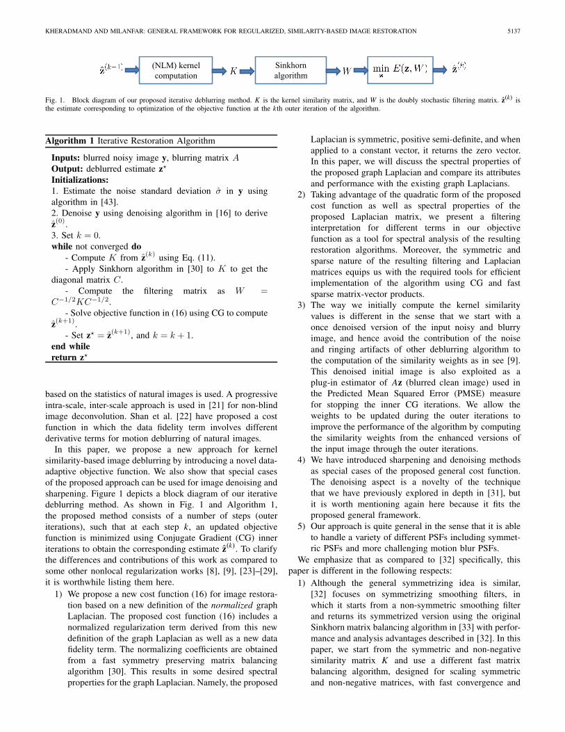
Fig. 1. Block diagram of our proposed iterative deblurring method. K is the kernel similarity matrix, and W is the doubly stochastic filtering matrix. z(k) isthe estimate corresponding to optimization of the objective function at the kth outer iteration of the algorithm.

Algorithm 1 Iterative Restoration Algorithm

based on the statistics of natural images is used. A progressiveintra-scale, inter-scale approach is used in [21] for non-blindimage deconvolution. Shan et al. [22] have proposed a costfunction in which the data fidelity term involves differentderivative terms for motion deblurring of natural images.

In this paper, we propose a new approach for kernelsimilarity-based image deblurring by introducing a novel data-adaptive objective function. We also show that special casesof the proposed approach can be used for image denoising andsharpening. Figure 1 depicts a block diagram of our iterativedeblurring method. As shown in Fig. 1 and Algorithm 1,the proposed method consists of a number of steps (outeriterations), such that at each step k, an updated objectivefunction is minimized using Conjugate Gradient (CG) inneriterations to obtain the corresponding estimate z(k). To clarifythe differences and contributions of this work as compared tosome other nonlocal regularization works [8], [9], [23]–[29],it is worthwhile listing them here.

1) We propose a new cost function (16) for image restora-tion based on a new definition of the normalized graphLaplacian. The proposed cost function (16) includes anormalized regularization term derived from this newdefinition of the graph Laplacian as well as a new datafidelity term. The normalizing coefficients are obtainedfrom a fast symmetry preserving matrix balancingalgorithm [30]. This results in some desired spectralproperties for the graph Laplacian. Namely, the proposed

Laplacian is symmetric, positive semi-definite, and whenapplied to a constant vector, it returns the zero vector.In this paper, we will discuss the spectral properties ofthe proposed graph Laplacian and compare its attributesand performance with the existing graph Laplacians.

2) Taking advantage of the quadratic form of the proposedcost function as well as spectral properties of theproposed Laplacian matrix, we present a filteringinterpretation for different terms in our objectivefunction as a tool for spectral analysis of the resultingrestoration algorithms. Moreover, the symmetric andsparse nature of the resulting filtering and Laplacianmatrices equips us with the required tools for efficientimplementation of the algorithm using CG and fastsparse matrix-vector products.

3) The way we initially compute the kernel similarityvalues is different in the sense that we start with aonce denoised version of the input noisy and blurryimage, and hence avoid the contribution of the noiseand ringing artifacts of other deblurring algorithm tothe computation of the similarity weights as in see [9].This denoised initial image is also exploited as aplug-in estimator of Az (blurred clean image) used inthe Predicted Mean Squared Error (PMSE) measurefor stopping the inner CG iterations. We allow theweights to be updated during the outer iterations toimprove the performance of the algorithm by computingthe similarity weights from the enhanced versions ofthe input image through the outer iterations.

4) We have introduced sharpening and denoising methodsas special cases of the proposed general cost function.The denoising aspect is a novelty of the techniquethat we have previously explored in depth in [31], butit is worth mentioning again here because it fits theproposed general framework.

5) Our approach is quite general in the sense that it is ableto handle a variety of different PSFs including symmet-ric PSFs and more challenging motion blur PSFs.

We emphasize that as compared to [32] specifically, thispaper is different in the following respects:

1) Although the general symmetrizing idea is similar,[32] focuses on symmetrizing smoothing filters, inwhich it starts from a non-symmetric smoothing filterand returns its symmetrized version using the originalSinkhorn matrix balancing algorithm in [33] with perfor-mance and analysis advantages described in [32]. In thispaper, we start from the symmetric and non-negativesimilarity matrix K and use a different fast matrixbalancing algorithm, designed for scaling symmetricand non-negative matrices, with fast convergence and


Fig. 2. Graph representation of images and construction of kernel similaritymatrix K , un-normalized Laplacian D − K and normalized LaplacianI − C−1/2 K C−1/2.

symmetry-preserving properties even when the matrixscaling algorithm is stopped early [30].

2) We use the symmetric and doubly stochastic outputof [30] to define the normalized Laplacian and we useit in a variational graph-based formulation for variousrestoration problems.

In the rest of the paper, we elaborate on the above mentionedproperties. In Section II, we summarize some of the existingnonlocal regularization restoration methods in a unified graphrepresentation framework. In Section III, we discuss how toderive the symmetric kernel similarity and filtering matricesas the main building blocks of our algorithm. In addition,we present an appropriate definition of normalized Laplacianmatrix for filtering purposes and discuss its spectral properties.Section IV is devoted to introducing the objective functionand the proposed procedure to optimize it in order to getthe final estimate. Section V discusses special cases of theproposed objective function introduced in Section IV for imagedenoising and sharpening. In Section VII, we verify the effec-tiveness of the proposed deblurring algorithm via a numberof synthetic and real experiments of deblurring color imagesfor both symmetric PSFs (Gaussian and out-of-focus PSFs)as well as nonlinear camera motion blurs. Final conclusionand discussion is provided in Section VIII. Throughout thepaper, vectors are represented by boldface small letters, andmatrices are shown by capital letters. Also, in iterative updateequations, subscript indices for vectors indicate inner iterationnumbers, whereas superscript indices represent outer iterationnumbers.

II. RELATED WORK

In this section, we summarize some of the existing methodsbased on the idea of nonlocal regularization in a graph-basedframework. We first clarify our notation and summarize someof the definitions mostly common in the nonlocal regulariza-tion approaches in the literature. As depicted in Fig. 2, anyimage can be defined as an intensity function on the vertices Vof a weighted graph G = (V , E, K ) consisting of a finiteset V of vertices (image pixels) and a finite set E ⊂ V × Vof edges (i, j) with the corresponding weights K (i, j) whichmeasure similarity between vertices (pixels) i and j in thegraph (e.g., Eq. 11). The function (intensity) values of theimage can be denoted as a vector1 z = [z(1), . . . , z(N)]T .

1Note that N = n2.

The similarity weights are represented as an N × N matrix K ,which is symmetric and non-negative.

As shown in Fig. 2, graph Laplacian matrix is derivedfrom K and plays an important role in describing the under-lying structure of the graph signal. There are three differentdefinitions of the graph Laplacian commonly used in the liter-ature in the context of graph signal and image processing, eachhaving different spectral properties [34]–[36]. In this paper, wepresent a fourth one, a new normalized graph Laplacian forimage processing purposes. In Table I, we have summarizedthe properties of different types of Laplacians used in theliterature along with those of our proposed definition.

In [23] and [37], the difference of a function z : V → �on an edge (i, j) ∈ E of the graph G is defined as:

(dz)(i, j) = √K (i, j)(z( j) − z(i)). (3)

Also, the weighted gradient vector of a function z at a vertexi ∈ V can be expressed as:

∇z(i) = [dz(i, j1), . . . , dz(i, jm)]T , ∀(i, j) ∈ E . (4)

Accordingly, the Laplace operator of z at a vertex i is derivedas:

�z(i) =∑

j, j∼i

K (i, j)(z(i) − z( j)). (5)

where j ∼ i stands for the vertices j in the graph such thatj is connected to i ; i.e., (i, j) ∈ E .

The authors in [23] and [37] propose a nonlocal regulariza-tion approach by considering the following cost function:

E(z, y, η) = ‖z − y‖2 + ηR(z), (6)

where the regularization functional R is:

R(z)= 1

2

N∑

i=1

‖∇z(i)‖2 = 1

2

N∑

i=1

∑

j, j∼i

K (i, j)(z(i) − z( j))2.

(7)

It essentially enforces the similar pixels of the image -asmeasured by the function K (., .)- to remain similar in thefinal estimate. By minimizing the above cost function withrespect to the unknown z, they recover the desired image. Notethat the regularization term (7) can be expressed based on theun-normalized graph Laplacian D − K as [23], [34], and [38]:

R(z) = zT (D − K )z, (8)

where D = diag{K 1N } is a diagonal matrix whose i thdiagonal element is the sum of the elements of the i throw of K , and 1N is the N-dimensional vector of all ones.In [23] and [37], the authors also introduce the Laplace oper-ator associated to the traditional normalized graph LaplacianI − D−1/2 K D−1/2. However, they do not use this definition ofthe Laplacian in their formulation because of the fact that theoutput of this operator is not null when the input is constant.

In [25], Gilboa and Osher consider the same nonlocalfunctional as the one in (6) for image denoising. Theydiscuss the case η = ∞ as well, for which they derive thediffusion flows (iterations) defined based on the un-normalized


TABLE I

PROPERTIES OF DIFFERENT GRAPH LAPLACIANS. LAST ROW IS OUR DEFINITION

Laplacian D − K . They show these types of iterations givebetter performance than the diffusion iterations correspondingto another type of normalized Laplacian (called random walkLaplacian and defined as I −D−1 K ). Also, in [26], the authorsintroduce the gradient-based and difference-based regularizingfunctionals, respectively as (we consider here their discreteversions):

J (z) =N∑

i=1

φ(‖∇z(i)‖2)

=N∑

i=1

φ(∑

j, j∼i

K (i, j)(z( j) − z(i))2), (9)

Ja(z) =N∑

i=1

∑

j, j∼i

φ(K (i, j)(z( j) − z(i))2), (10)

in which φ(s) is a positive function, convex in√

s, withφ(0) = 0. They consider the quadratic case φ(s) = s, wherethe above functionals coincide. They also investigate the caseφ(s) = √

s, for which nonlocal TV and anisotropic nonlo-cal TV functionals are derived from the gradient-based anddifference-based approaches, respectively. They have appliedtheir framework to inpainting and detecting and removingirregularities from textures.

In [28], Szlam, Maggioni, and Coifman propose functionadapted diffusion processes (using the random walk LaplacianI − D−1 K ). They also propose a filtering procedure using atype of thresholding of the expansion coefficients of the inputfunction on the linearly independent bases of the operatorD−1 K . Reference [29] is also based on the same idea(expansion of the input data on the space spanned by the righteigenvectors of random walk Laplacian) for surface smoothingwith weights derived locally in a non data-adaptive manner.The denoising method in [27], exploits a similar filteringidea as in [28]; i.e., constructing a weighted graph fromthe input image characterized by its normalized LaplacianI − D−1/2 K D−1/2, and expanding the noisy image using theorthonormal bases of the normalized graph Laplacian, thenhard thresholding of the transform coefficients to derive thecorresponding estimates for image pixel intensities in differentpatches of the image. In [24], a patch-based functional isconsidered for denoising 3D image sequences acquiredvia fluorescence microscopy. This functional is based onminimizing a difference penalty term which is defined usingthe weighted difference between its patches rather than theweighted difference between its pixels. The minimizer of sucha cost function can be equivalently expressed as a nonlocalfiltering process; i.e., z = D−1 K y.

Finally, the most relevant paper to our work is reference [9],in which Zhang et al. propose two efficient algorithms forsolving nonlocal TV-based image deconvolution.2 They alsoprovide a weight updating strategy within these iterativemethods which was found to be ineffective in improving theperformance of their algorithms. Therefore, they chose tocompute the similarity weights only once from the simpleTikhonov regularization based deblurring estimate. Also, [8]proposes a regularization technique using total variation onnonlocal graphs for inverse problems, when the input datahas undergone linear degradation as well as additive noise.Note that our deblurring algorithm uses a different nonlocalapproach, in which the corresponding regularization termis defined using the normalizing coefficients derived fromSinkhorn’s algorithm in [30]. Moreover, based on our exper-iments, the weight updating strategy is indeed effective inimproving the performance of the proposed algorithm withinthe same quadratic framework. Furthermore, according to theanalysis provided in [22], using the data fidelity term involvingdifferent derivatives of the residual is better able to model theunderlying process for deblurring problems (especially for realmotion blurred images).

III. DERIVATION OF BUILDING BLOCK MATRICES

OF THE PROPOSED ALGORITHM

In this section, we introduce the kernel similarity matrix Kand a closely related doubly stochastic symmetric matrix Was the main filtering building block of our iterative algorithmfrom a graph point of view. Having these matrices at hand,we can define the normalized Laplacian matrix whose spec-tral properties are crucial for analyzing the behavior of thealgorithm.

A. Kernel Similarity Matrix K and Filtering Matrix W

While our approach is general enough to include any validkernel similarity function [39], [40], the (i, j)th element of thekernel similarity matrix K is computed here using the nonlocalmeans (NLM) definition as [41]

K (i, j) = exp(−‖zi − z j‖2

h2 ), (11)

in which zi and z j are patches around the pixels i and j ofthe image z, and h is a smoothing parameter. Note that at eachouter iteration, the kernel similarity weights are re-computedfrom the estimate at the previous iteration. As a result of the

2As mentioned, the corresponding regularization term is derived usingφ(s) = √

s in Eq. (9).


above definition for the kernel similarity weights, the matrix Kwould be a symmetric non-negative matrix. Furthermore, weonly compute the similarity between each patch and a smallneighbourhood of patches around it (e.g., a search window ofsize 11 × 11 of patches around each patch). Therefore, thematrix K is sparse. This sparse structure is appealing from acomputational point of view.

Applying Sinkhorn matrix balancing procedure [33] to thematrix K yields the doubly stochastic filtering matrix W .We use a recent fast version of the original algorithmfor symmetric non-negative matrices [30]. This balancingalgorithm returns a diagonal scaling matrix C , such thatthe resulting matrix W = C−1/2 K C−1/2 is a symmetricnon-negative doubly stochastic matrix. Since W is symmetric,it can be decomposed as W = V SV T , where V is anorthonormal matrix whose columns are the eigenvectorsof W , and S = diag{λ1, λ2, . . . , λN } is a diagonal matrixconsisting of eigenvalues of W as its diagonal elements.Moreover, since W is doubly stochastic, it has eigenvaluesin the range λ1 = 1 > λ2 ≥ · · · ≥ λN ≥ 0 [40]. The largesteigenvalue is exactly equal to 1 with the corresponding DCeigenvector v1 = (1/

√N )[1, 1, . . . , 1]T = (1/

√N )1N [40].

Intuitively, it means that applying W to a signal, preservesthe DC component of the signal. This is a desirable propertyfor filtering purposes. Note that the spectral analysis of thematrix W reveals its inherent low-pass nature (the largesteigenvalue corresponds to the DC component) [32].

B. Normalized Graph Laplacian Matrix

At this point, we define our normalized graph Laplacianmatrix as

I − W = I − C−1/2 K C−1/2. (12)

This is the proper definition of the normalized graphLaplacian matrix for image filtering purposes, as opposedto its traditional definition in graph theory literatureI − D−1/2 K D−1/2 [34], [38]. It is worthwhile comparingthis traditional definition of the normalized Laplacian withour proposed definition which is based on a very differentscaling of the similarity matrix K using matrix balancing [30].Our definition of the normalized Laplacian (I − W =I − C−1/2 K C−1/2) is symmetric, positive semi-definite, withthe zero eigenvalue associated to the constant eigenvector

1√N

1N . Hence, when applied to a constant function, it returnsa zero vector. The traditional definition of the normalizedgraph Laplacian lacks the desired filtering property of havingDC eigenvector as one of the basis eigen functions [34].As a result, the definition of normalized graph Laplacianin (12) is proposed and used in this paper. This definitionhas the desired spectral properties for our specific applicationsas well as a nice filtering interpretation. In fact, the setof eigenvectors of I − W can be considered as the basisfunctions of the underlying graph, and its eigenvalues canbe thought of as the corresponding graph frequencies. Also,note that the Laplacian I − W has a high-pass filtering nature(with null eigenvalue corresponding to the DC eigenvector).This property is consistent with the expected behavior of

the Laplacian filter in image processing. Consequently, whenapplied to an image, I − W can be directly interpreted asa data-adaptive Laplacian filter. Therefore, it enables us toincorporate different types of filters in the data term coupledto the regularization term based on the application at hand.In the “random walk” Laplacian I − D−1 K , (from the theoryof Markov chains), the (i, j)th element of D−1 K representsthe probability of moving from node i to node j of the graphin one step, given that we are in node i [42]. A similar randomwalk interpretation can be provided by our symmetric doublystochastic filtering matrix W = C−1/2K C−1/2, with analysisand performance advantages over D−1 K for image filtering,as discussed in [32].3 Furthermore, for image deblurringapplications, another advantage is that our resulting linearequations are symmetric and positive definite, providing uswith fast methods for solving large linear systems of equationswith optimization methods like CG. Compared to the un-normalized graph Laplacian, as we have shown in [31], ourapproach based on the proposed normalized graph LaplacianI − W provides better performance.

In order to better demonstrate the different expressions ofthe difference and Laplacian operators as well as the regu-larization term corresponding to our normalized Laplacian,we derive them here. We can define the difference operatorcorresponding to the proposed normalized graph Laplacian as:

dz(i, j) = √K (i, j)(

z( j)√C( j, j)

− z(i)√C(i, i)

), (13)

where C( j, j) and C(i, i) are the corresponding j andi th diagonal elements of the diagonal matrix C derivedfrom the matrix balancing algorithm [30], [32]. Fromthe above equation along with the definition of the divergenceoperator [23], the Laplace operator corresponding to thenormalized Laplacian I − C−1/2 K C−1/2 is:

z(i) = 1√C(i, i)

∑

j, j∼i

K (i, j)(z(i)√C(i, i)

− z( j)√C( j, j)

), (14)

As a result, our proposed regularization term can be written as:

R(z) = 1

2

N∑

i=1

∑

j, j∼i

K (i, j)(z(i)√C(i, i)

− z( j)√C( j, j)

)2

= zT (I − W )z. (15)

Note that the Laplace operator in (14) describes the effectof our normalized Laplacian at each pixel i , when applied toan input vector z. As the Laplace operator is a second orderderivative operator, the name Laplacian for the correspondingmatrix operator is appropriate, and common in graph theory.In the next section, we will describe how to use the proposedgraph Laplacian to develop a new restoration algorithm.

IV. PROPOSED DEBLURRING METHOD

As depicted in Fig. 1, the proposed algorithm consists ofinner and outer iterations. The reason is that for computingthe data-adaptive matrix K , a good rough estimate of the

3In fact, W can be thought of as the transition probability matrix of theMarkov chain defined on the graph.


underlying unknown image is needed. This estimate is gradu-ally improved as we proceed through iterations. In each outeriteration, the matrix W is computed once and used to definethe following objective function to be minimized with respectto the unknown image z

E(z) = (y − Az)T {I + β(I − W )}(y − Az)

+ η zT (I − W )z, (16)

where β ≥ −1 and η > 0 are the parameters to be tunedbased on the amount of noise and blur. Note that in theabove objective function, data and prior terms are coupledvia the matrix W . This coupling is controlled by means of theparameter β. The first term favors a solution z such that itsblurred and then filtered version is as close as possible to thefiltered version of the input y. Frequency selectivity of thiscommon filter is determined by the parameter β accordingto the amount of the noise and blur. The second term isessentially a data-adaptive difference term favoring certainsmoother solutions based on the structure of the underlyingdata encoded in the normalized Laplacian matrix I − W ,defined in the previous section.

Let us take a look at the cost function in (16) from afiltering point of view. This filtering interpretation providesa more intuitive perspective on the objective function. For thispurpose, Eq. (16) is rewritten in the following form

E(z) = ‖{I + β(I − W )}1/2(y − Az)‖2

+ η‖(I − W )1/2z‖2. (17)

Note that I + β(I − W ) = V �V T is a symmetric andpositive semi-definite matrix. Therefore, the matrix {I + β(I−W )}1/2 = V �1/2V T has a filtering behavior similar to thatof I +β(I −W ). Once we have the eigendecomposition of thefiltering matrix W , the i th diagonal element of the matrix �can be written in terms of the associated i th diagonal elementof S (that is λi ) as 1 + β(1 − λi ). Since the matrix I − Wis a high-pass filter, with β > 0, I + β(I − W ) behaves likea sharpening filter on the residuals y − Az, and so does {I +β(I − W )}1/2. According to the analysis provided in [22],using the data fidelity term involving different derivatives ofthe residual is better able to model the underlying phenomenonfor deblurring problems (especially for real images).

The same analysis applies to the second term in (17), whereboth Laplacian I −W , and its square root (I −W )1/2, are adap-tive high-pass filters. Consequently, the resulting regularizationexpression in (17) adaptively penalizes high frequencies inthe final solution to avoid unpleasant artifacts due to thenoise amplifications and ringing artifacts while maintainingfine details in the restored image.

In order to minimize the cost function in (16) at each step,the corresponding gradient is set equal to zero as

∇E(z) = −2AT {I + β(I − W )}(y − Az)

+ 2η(I − W )z = 0, (18)

which results in the following symmetric positive definitesystem of liner equations

(AT {I + β(I −W )}A + η(I − W ))z = AT {I +β(I −W )}y.

(19)

TABLE II

CONDITION NUMBER OF (AT (I + β(I − W ))A + η(I − W )) FOR

DIFFERENT VALUES OF η AND β AND BLURRING MATRIX A

CORRESPONDING TO OUT-OF-FOCUS BLUR WITH RADIUS 7.

THE CONDITION NUMBER OF AT A IS 5.74 × 1020

Conjugate Gradient is then used to solve the above system.Also, note that A and AT are interpreted as blurring with thePSF or its flipped version, respectively. Our experiments showthat three outer iterations suffice to get the desired deblurredoutput in most cases. Also, note that the only restrictionon the parameter β is that it should be selected such thatthe corresponding system of linear equations in (19) remainspositive definite. The matrix I + β(I − W ) is also required tobe positive semi-definite for the existence of its square root inthe data fit term in (17). A sufficient condition is β ≥ −1.

A. Spectral Analysis of the Overall Deblurring Algorithm

For analysis purposes, we are able to provide a filteringinterpretation of the final estimate at each outer step of thealgorithm. Note that the minimizer of the cost function in (17)can be expressed as:

z = F(A, W )AT (I + β(I − W ))y, (20)

where

F(A, W ) = {AT (I + β(I − W ))A + η(I − W )}−1. (21)

Eq. (20) can be interpreted as (1) filtering y by I +β(I − W ),(2) back projection through multiplication by the transpose ofthe blurring matrix A, and (3) applying the symmetric matrixF(A, W ). In other words, if we consider the spectral decom-position of this symmetric matrix as F(A, W ) = ϒT , thecolumns of the matrix serve as an orthonormal basis forfiltering the vector AT (I + β(I − W ))y, thereby providing aspectral filtering interpretation for the corresponding deblur-ring solution at each outer step of the algorithm. Since aninverse operation is involved in (20), we consider a simpleexperiment investigating the condition number of the matrixAT (I + β(I − W ))A + η(I − W ). For this purpose, we usethe MATLAB code in [44] to explicitly construct the blurringmatrix A related to out-of-focus blur with radius 7. Table IIillustrates the condition number of AT (I + β(I − W ))A +η(I − W ) for different values of the parameters η and β. Thecondition numbers of AT (I + β(I − W ))A + η(I − W ) fordifferent values of η in comparison to the condition numberof AT A show the effectiveness of our procedure for regular-izing the ill-posed deblurring problem and the correspondinglinear equations. Also, the basis eigenvectors in correspond-ing to the four largest eigenvalues of F(A, W ) are depictedin Fig. 3. As can be seen in Fig. 3, the eigenvectors asso-ciated with the largest eigenvalues of F(A, W ) indicate thedata-adaptive nature of the corresponding filter.


Fig. 3. (a) Original 41 × 41 image, and (b), (c), (d), (e) the eigenvectorsof F(A, W ) corresponding to the four largest eigenvalues for β = 0.7 andη = 0.2.

V. SPECIAL CASES OF THE PROPOSED

OBJECTIVE FUNCTION

It is interesting to consider two special cases of the aboveobjective function in (16) for two different applications,namely denoising and sharpening.

A. Image Denoising

When A = I in (16), the problem reduces to that ofimage denoising. This case has been discussed in our previouswork [31]. It turns out that β = −1, is the appropriatechoice for image denoising [31]. Also, the optimal value ofthe regularization parameter η is selected using a SURE-basedestimated MSE approach [45]. The proposed denoising formu-lation is able to describe some of the existing kernel similarity-based denoising algorithms, and provides an iterative approachfor their further improvement [31].

B. Image Sharpening

Another special case is when image contains a moderateblur, but no information about the blurring process is avail-able. In such cases, one can resort to the following costfunction

E(z) = (y − z)T {I + β(I − W )}(y − z), (22)

which comes from Eq. (16), by setting A = I and η = 0.Optimizing the above objective function using simple

steepest descent, yields:

z� = z�−1 + μ{I + β(I − W )}(y − z�−1). (23)

By selecting the step size parameter μ = 1, and with zeroinitialization of the SD iterations in (23); i.e., z0 = 0, the firstiteration takes the form

z1 = {I + β(I − W )}y. (24)

For β > 0, Eq. (24) can be interpreted as data-adaptivelyadding to the input image some amount of its high-pass filteredversion. This procedure results in a sharper image. Althoughthere is no access to the exact PSF, since the matrix Wis computed from the input blurred image, it containssome information about the original image as well asthe blurring process. Therefore, Eq. (24) provides us witha data-adaptive sharpening (or to say rough deblurring)technique.

VI. IMPLEMENTATION DETAILS

The first step of the iterative algorithm is to compute thekernel similarity matrix4 K . At each outer iteration k, wecompute this matrix from the final estimate of the previousstep, i.e., from z(k−1), as shown in Fig. 1. The values ofthe regularization parameters η and β are selected based onthe noise variance and blurring scenario, and are kept fixedat each step of the algorithm, for all the test images. Fordeblurring examples, for instance, the parameter β lies in therange (0, 1), and the parameter η is empirically selected in therange (0, 0.4). The closer is β to 1, the larger is the effect ofthe data-adaptive high-pass filter I + β(I − W ) in the dataterm of the cost function in (16), which results in encouraginghigher frequencies of Az to be close to those of y. Similarly,the larger is the value of η, the more penalty is put on the normof the high-pass filtered version of the desired solution z. Forinstance, larger values of η and smaller values of β are usedwhen the amount of noise is high in the input image, and theimage is moderately blurred. Similarly, when the amount ofnoise is low while the image is severely blurred, larger valuesof β and smaller values of η are used. These tunings are donefor each scenario of blur and noise for a set of test images tohave visually pleasant results, and are kept fixed for all otherinput images with the same degree of degradation, as shownin the next section.

To further speed up the convergence of the iterativealgorithm, each step of the algorithm is initialized with thecorresponding estimate from the previous step. In experiments,in order to avoid noise amplification and ringing artifacts,the maximum number of inner and outer iterations areset beforehand based on the amount of degradation,5 andthen the iterations are stopped using a rough estimate ofPredicted-MSE (PMSE) measure as6

P M SE(q, k) = 1

n2 ‖ Az − Az(q)k ‖2, (25)

where Az is an estimate of the blurred clean image (Az),which is derived by denoising input noisy blurry image, andz(q)

k is the corresponding estimate of the desired image at thekth CG iteration of the qth outer iteration. That is, we stopCG iterations whenever P M SE(q, k + 1) > P M SE(q, k).

There are two main computational burdens for thealgorithm. First is the computation of the kernel similaritycoefficients, where its special form allows us to takeadvantage of the idea of integral images [47]. This techniqueis very effective to reduce the computational complexityof the algorithm. Second is the matrix-vector productsrequired at each iteration of CG method for optimizing theobjective function in (16). However, because of the specialstructure of the matrices involved, it is possible to implementthe algorithm using Fast Fourier Transform (FFT) and fast

4This is computed from the denoised version of the input image at thebeginning of the algorithm.

5For more blurry images, we need more iterations for convergence of CGiterations. Also, as we initialize the CG iterations with more enhanced imagesas we proceed through the outer iterations, the number of inner iterations isdecreased by a step nDec, as the number of outer iterations increases.

6Predicted-MSE is defined as P MS E(q, k) = 1n2 ‖A(z − z(q)

k )‖2 [46].


Fig. 4. Set of color images used for evaluation of our method: (a) Building image (480 × 640), (b) Motocross bikes image (494 × 494), (c) Girl image(496 × 700), (d) Street image (480 × 640), (e) Boat image (420 × 520), and (f) Book shelf image (580 × 520).

sparse matrix-vector products. It is also possible to exploitthe symmetric structure of the kernel similarity matrix K(and of course that of W ) to reduce memory requirements.

VII. NUMERICAL EXPERIMENTS

In this section, the effectiveness of our iterative approach isverified through a number of synthetic and real experiments.Throughout the deblurring experiments, our focus is on morepractical cases with severe blur and small amount of noise inthe captured images. We have set up experiments for Gaussian,out-of-focus, and nonlinear camera motion blur. For all cases,we have compared the performance of our algorithm withsome of the best existing non-blind deblurring algorithms.Also, for both motion and out-of-focus blurs, the iterativealgorithm is applied to real images to evaluate its performancefor such more complicated cases. Since the proposed methodis a non-blind deblurring algorithm, for real deblurringexamples, we use PSFs derived from other existing blurkernel estimation methods. For this purpose, in case of realout-of-focus blur, the PSF is estimated using “deconvblind”MATLAB function. In case of real motion deblurring, theestimated PSFs from [22] and [48] are used. Furthermore,synthetic and real image sharpening examples are provided.For color images, the proposed deblurring algorithm is appliedindependently to R, G, and B channels of the input color imageto get the final estimate. In all the experiments, object orientedMATLAB functions in [49] are used for performing matrix-vector products of the form Az and AT z. PSNR in dB andthe SSIM index are used for comparison purposes [50].SSIM index is shown to be a more reliable metric forcomparison of deblurring algorithms than the widely usedPSNR measure [50]. In order to show the effectivenessof our proposed method compared to one of the existingapproaches based on nonlocal means regularization for imagedeconvolution [9], we first demonstrate deblurring examplesrelated to this comparison.

A. Comparison With Nonlocal Means RegularizationDeconvolution Algorithm

In the following experiments, Cameraman image iscircularly convolved with box average and motion blurs, andwhite Gaussian noise with standard deviation σ = 1 is addedto generate the noisy blurred examples. The regularizationparameters of both algorithms are selected for the bestperformance in each case.7 For the next deblurring example

7We use the MATLAB and mex codes provided by the authors inhttp://www.math.ucla.edu/∼xqzhang/html/code.html.

with nonlinear motion blur and the same noise level (σ = 1),the regularization parameter μ of the algorithm in [9] andthe parameters η and β in our algorithm are changed and theother parameters in both algorithms remain the same as thefirst experiment. Note that for fair comparisons, we are usingthe same definition of the nonlocal similarity function asthe one in [9] and [41] with the corresponding Gaussianweighting for the patch elements.

For box average blur kernel, as can be seen from the resultsin Fig. 5, while our method gives slightly better visual quality,both algorithms show comparable quantitative performance.However, for nonlinear motion blur, the algorithm in [9] almostfails with the current settings provided by the authors asshown in Fig. 6, while our proposed algorithm shows superiorperformance in this case in terms of both PSNR and SSIMvalues. This is due to our definition of the cost function, andthe new normalized regularization term as well as a differentdata fit term. This good performance can also be attributedto the way we initialize the algorithm, such that we do notcompute the weights from the output of another deblurringalgorithm to avoid contributing the deblurring artifacts to thesimilarity weights. Instead, we allow the weights to be updatedas we proceed through iterations.

B. Symmetric Blurs

Two kinds of symmetric blur are considered for theseexamples: Gaussian blur and out-of-focus blur. A 25 × 25Gaussian blur with standard deviation 1.6 is convolved with aset of color images8 shown in Fig. 4. Also, out-of-focus bluris produced using a disk function with radius 7 and is used togenerate the corresponding blurred examples. Then, additivewhite Gaussian noise with variances equal to 0.2 and 1 isadded to the blurred images. We compare the performanceof our algorithm with that of IDDBM3D algorithm in [18].Periodic boundary conditions are used in these examples [1].Also, we use patch size of 5 × 5, search neighborhood sizeof 11 × 11, number of outer iterations equal to 3, and thestep decrement of the number of inner iterations (nDec) equalto 30 in these experiments. The values of the parametersη, β, h, and maximum number of inner CG iterations havebeen summarized in Table IV. Note that, the parameters ofboth algorithms are set for best performance in each case forthis set of images, and for the given blurs and noise variances.

Figures 7 and 8 depict deblurring outputs of our algorithmcompared to those of IDDBM3D for noise variance of 0.2

8Test images are from Kodak Lossless True Color Image Suite(http://r0k.us/graphics/kodak/) and the web page for [51].


Fig. 5. Deblurring example with noisy blurred Cameraman image with 9 × 9 box average blur kernel and additive white Gaussian noise with standarddeviation σ = 1: (a) clean image, (b) blurred noisy image, (c) output of [9] with regularization parameter μ = 14 in the algorithm (PSNR = 27.43dB,SSIM = 0.8544), and (d) output of our proposed deblurring algorithm with η = 0.02 and β = 5 × 10−4 (PSNR = 28.02dB, SSIM = 0.8537).

Fig. 6. Deblurring examples with blurred noisy Cameraman image with nonlinear motion blur and additive white Gaussian noise with standard deviationσ = 1: (a) clean image, (b) blurred noisy image, (c) output of [9] with the regularization parameter μ = 80 in the algorithm (PSNR = 16.82dB,SSIM = 0.3969), and (d) output of our proposed deblurring algorithm with η = 0.022 and β = 0.2 (PSNR = 27.94dB, SSIM = 0.8581).

TABLE III

SSIM AND PSNR PERFORMANCE OF THE KERNEL SIMILARITY-BASED ALGORITHM AND IDDBM3D [18] FOR GAUSSIAN BLUR KERNEL OF SIZE

25 × 25 WITH STANDARD DEVIATION 1.6 AND OUT-OF-FOCUS BLUR GENERATED USING DISK FUNCTION OF RADIUS 7. IN EACH CELL,

THE FIRST NUMBER DENOTES SSIM VALUE, AND THE SECOND NUMBER REPRESENTS PSNR VALUE IN DB

TABLE IV

SET OF PARAMETERS IN DIFFERENT SYNTHETIC COLOR IMAGE

DEBLURRING EXAMPLES IN THIS PAPER. NINNER IS THE

MAXIMUM NUMBER OF THE INNER CG ITERATIONS

and synthetic Gaussian and out-of-focus blurs, respectively.Also, Table III summarizes the numerical deblurring results.As can be seen in Table III, our kernel similarity-basedalgorithm shows very close performance to the state-of-the-artIDDBM3D algorithm in [18] in the case of Gaussian blur.

Also, our iterative algorithm performs acceptably in the caseof out-of-focus blur. In some cases, our algorithm exhibitsslightly better visual quality as can be seen, e.g., in smoothparts of the face of the Girl image in Fig. 8. There is one keydifference between our proposed algorithm and IDDBM3D.IDDBM3D is a two step algorithm, in which denoising anddeblurring are decoupled. Each step of IDDBM3D essentiallyinvolves solving two different objective functions, one fordeblurring and the other for denoising. Regarding the com-putational complexity, even though our algorithm has beenwritten entirely in MATLAB (except the initial denoisingstep which we use the code provided by the authors in [16]),9

our algorithm runs faster, making it more appropriate for

9In contrast, the computational demanding parts of IDDBM3D have beenimplemented in C++ using MATLAB mex files.


Fig. 7. Deblurring example with Gaussian blur: (a) clean Motocross bikes image, (b) blurred noisy image, (c) output of [18], and (d) output of our algorithm.

Fig. 8. Deblurring example with out-of-focus blur: (a) clean Girl image, (b) blurred noisy image, (c) output of [18], and (d) output of our algorithm.

practical image deblurring applications. To be more specific,for a 480×640 color image, the MATLAB implementation ofour kernel similarity-based method runs 4 times faster than thecode for IDDBM3D run on a 2.8 GHz Intel Core i7 processor.Furthermore, our method just relies on an initial denoising,whereas IDDBM3D depends on an appropriate estimate fromanother deblurring algorithm in its grouping phase. In addition,as we demonstrate in the remaining experiments, the proposedmethod has the flexibility to be applied to a wide varietyof blurs including both symmetric and non-symmetric blurs,while IDDBM3D has been designed and tested specifically forsymmetric blurs.

Figure 9 shows the output of our algorithm when appliedto real noisy and out-of-focus blurred images compared to theoutputs of the Focus Magic deblurring software. As can beseen, our algorithm is better able to handle noise amplificationrelated issues. In the following subsections, we consider theeffect of different factors on the performance of the proposeddeblurring method.

1) Effect of the Patch Size on the Performance of theProposed Algorithm: In this subsection, we add an experimentinvestigating the relationship between the patch size and blurkernel width in the deblurring algorithm for the case of

out-of-focus blur. Synthetic examples are produced by apply-ing out-of-focus blur kernels with radii 5, 7, 9, and 11 to theGirl image. White Gaussian noise with variance σ 2 = 0.4 isalso added to the blurred images. The corresponding SSIMvalues are plotted in Fig. 10 versus the patch size for differentradii of the out-of-focus blur.10 It can be seen that for out-of-focus blur, the best performance is not strongly dependent onthe patch size regardless of the out-of-focus blur kernel radius.It shows that for such blur kernels, the structure around eachpixel is described well just by considering a small 5×5 patcharound it. In other words, there is no specific relation betweenthe patch size and the size of the blur kernel. In fact, onecan fix this parameter and change other parameters like theregularization parameter η to control the quality of the outputimage.

2) Effect of the Smoothing Parameter h on the Performanceof the Proposed Algorithm: In order to investigate the effectof the parameter h, we apply out-of-focus blur with radius 7to the clean Girl image and then add noise with two differentvariances (0.2 and 1) to it. The results are shown in Fig. 11.Note that the same set of parameters are used for both cases

10We consider patch sizes 3, 5, and 7.


Fig. 9. Real sharpening examples: left column: input blurred noisy image, middle column: output of Focus Magic software at http://www.focusmagic.com,and right column: output of our algorithm (η = 0.1 and β = 0.06 for both images).

Fig. 10. The relationship between the patch size and blur kernel width forGirl image and out-of-focus blur with different radii.

Fig. 11. The effect of the smoothing parameter h in the kernel similarityfunction for Girl image and out-of-focus blur with radius 7 for two differentnoise variances.

of noise variance. As can be seen, with the same set ofparameters, the optimal smoothing parameter h is greater forthe higher noise level. Also, it is evident from Fig. 11 that

Fig. 12. Convergence plots of the CG iterations for different initializations.

the algorithm is not very sensitive to the selection of thisparameter.

3) Effect of the Initialization of the CG Iterations on thePerformance of the Algorithm: In order to investigate the effectof the specific initialization for CG iterations at first step ofthe deblurring algorithm, we consider a simple experimentwith Girl image for Gaussian blur with standard deviation1.6 and noise variance σ 2 = 1. We consider two differentinitializations, of CG iterations with (1) the denoised version ofthe input noisy and blurred image versus (2) initializing it withzero image, i.e., z0 = 0. As can be seen in Fig. 12, in case ofinitializing with the denoised image, the algorithm convergesfaster. However, with simple zero initialization, we obtainthe same result only after more CG iterations. The proposedalgorithm is not sensitive to the initialization.

4) Effect of Oracle Scenario on the Performance of theProposed Algorithm: It is instructive to show reconstructionsstarting from the oracle scenario where the true images areused for the weights and applied to noisy data. we considera deblurring scenario in which test images are synthetically


TABLE V

PSNR ORACLE PERFORMANCE OF THE PROPOSED

ALGORITHM VS. THE LOW-NOISE CASE

TABLE VI

ISNR VALUES FOR THE GIRL IMAGE AND OUT-OF-FOCUS BLUR WITH

DIFFERENT NOISE STANDARD DEVIATION WHEN THE WEIGHTS ARE

COMPUTED FROM THE INPUT NOISY BLURRED IMAGE

blurred with 25 × 25 Gaussian blur kernel with standarddeviation 1.6 and the additive white Gaussian noise withvariance 0.4 is added. Then, we compare the performanceof the proposed algorithm, when the similarity weights arecomputed from the oracle images compared to the cases whenthese weights are derived from the given input (blurred, noisy)images. The results are summarized in Table V. As expected,using the oracle image for computing the similarity weightsimproves the performance of the algorithm. Also, it can beseen that for practical cases when the amount of noise is low,the results of the algorithm are not much different from theiroracle counterparts.

5) Effect of the Noise Level in the Computation of theSimilarity Weights: We add an experiment consideringthe effect of noise in computing the similarity weights.The Girl image is blurred by out-of-focus blur (of radius 7),and different amounts of noise (up to standard deviationequal to 30) are added to the blurred image. We fix all theparameters for different noise levels except the regularizationparameter η which is changed proportional to the noisestandard deviation as h = 0.05σ . In all the experiments, thesimilarity weights are computed from the noisy blurred inputimage in the first step of the algorithm. Table VI shows theISNR values for different noise levels.11 As can be seeneven for very high noise levels and with computation of theweights from the input image, the algorithm is able to provideimprovement with respect to the input degraded image.Although one can assume that the algorithm will fail at somenoise level, we can conclude that it is robust enough to theerrors in the input image for computing the similarity weights.

C. Synthetic Motion Blur

For assessing the performance of the algorithm in caseof motion deblurring, we use the complex camera motionblur kernel provided by Shan et al. [22]. Again, noise withvariances equal to 0.2 and 1 is added to the blurred images.In this case, we compare the proposed algorithm with two ofthe best available non-blind motion deblurring works. Periodicboundary conditions are used in these examples [1]. Also, weuse patch size of 5 × 5, search neighborhood size of 11 × 11,

11ISNR is defined as the difference between the PSNRs of the output imageand the input noisy blurred image.

TABLE VII

SSIM AND PSNR PERFORMANCE OF THE KERNEL SIMILARITY-BASED

ALGORITHM IN COMPARISON WITH THOSE OF MOTION DEBLURRING

METHODS IN [20] AND [22] FOR SYNTHETIC CAMERA MOTION BLUR.

IN EACH CELL, THE FIRST NUMBER DENOTES SSIM VALUE,

AND THE SECOND NUMBER REPRESENTS PSNR VALUE

number of outer iterations equal to 3, and the step decrementof the number of inner iterations (nDec) equal to 30 in theseexperiments. The values of the parameters η, β, h, and max-imum number of inner CG iterations have been summarizedin Table IV. The parameters of all algorithms are set for bestperformance. Table VII illustrates the quantitative results inthis case. From the numerical results in Table VII, it is evidentthat our proposed kernel similarity-based algorithm shows verygood performance in the case of non-blind nonlinear motiondeblurring.

D. Real Motion Deblurring

Now, we deal with more challenging motion blur situationswhere the blur kernel is estimated using two of the existingblur kernel estimation methods [22], [48] from real motionblurred test images. The estimated blur kernels are usedindependently to derive the final deblurred images. Theperformance of the proposed method is compared with thoseof [20] and [22], which are among the best non-blind motiondeblurring methods.

For all examples, the patch size and search window size areselected to be 5 × 5 and 11 × 11, respectively. Also, we usereflective boundary conditions for these experiments [1], [49].Figures 13 and 14 show the outputs of different methods, whenthe blur kernels are estimated using the algorithm in [22]. Also,Figures 15 and 16 illustrate the results of different algorithmswhen applied to real blurred images using correspondingestimated blur kernels from [48]. As can be seen, our iterativedeblurring algorithm produces high quality outputs as good asthe state-of-the art.

E. Comparison to Traditional Normalized Graph LaplacianThrough Image Deblurring Experiments

In order to compare the performance of our proposedalgorithm with the traditional normalized Laplacian(I − D−1/2 K D−1/2) formulation, we consider the followingdeblurring experiments. In these experiments, we first


Fig. 13. Real motion deblurring example: (a) input blurred noisy image, (b) Output of hyper-Laplacian algorithm [20], (c) output of [22], and (d) output ofour algorithm (η = 0.031, β = 0.6).



convolve the Girl image with Gaussian blur (standarddeviation equal to 1.6) and add white Gaussian noise withstandard deviation σ = 1 to it. Then, we use the proposed

deblurring algorithm to get the desired estimate. Also, weconsider a similar cost function to the one in (16) using thetraditional normalized Laplacian I −WD = I −D−1/2 K D−1/2



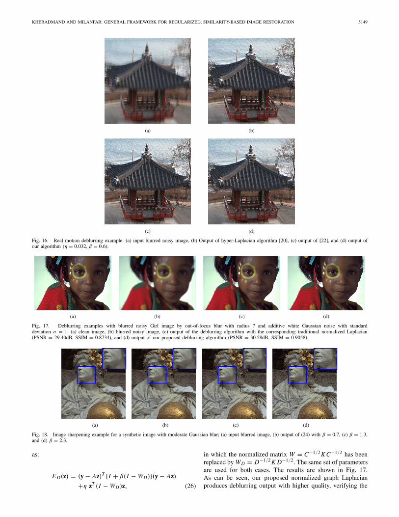
Fig. 17. Deblurring examples with blurred noisy Girl image by out-of-focus blur with radius 7 and additive white Gaussian noise with standarddeviation σ = 1: (a) clean image, (b) blurred noisy image, (c) output of the deblurring algorithm with the corresponding traditional normalized Laplacian(PSNR = 29.40dB, SSIM = 0.8734), and (d) output of our proposed deblurring algorithm (PSNR = 30.58dB, SSIM = 0.9058).

Fig. 18. Image sharpening example for a synthetic image with moderate Gaussian blur; (a) input blurred image, (b) output of (24) with β = 0.7, (c) β = 1.3,and (d) β = 2.3.

as:

ED(z) = (y − Az)T {I + β(I − WD)}(y − Az)

+η zT (I − WD)z, (26)

in which the normalized matrix W = C−1/2 K C−1/2 has beenreplaced by WD = D−1/2 K D−1/2. The same set of parametersare used for both cases. The results are shown in Fig. 17.As can be seen, our proposed normalized graph Laplacianproduces deblurring output with higher quality, verifying the


Fig. 19. Sharpening example for a real image; (a) input image and(b) sharpened image using our algorithm (β = 1.3).

superiority of the proposed normalized graph Laplacian withrespect to its traditional counterpart.

F. Image Sharpening Examples

There are many circumstances in which the image hasundergone moderate amount of blurring and there is no explicitknowledge of the blurring kernel available. In such cases, itis possible to exploit the data-adaptive sharpening frameworkin Section V to produce a sharper and more pleasant outputfrom the slightly degraded input image. In this case, thesharpened images derived through our kernel similarity-basedmethod have been shown in Fig. 18 for synthetic test imagesand different values of the parameter β. As can be seen inFig. 18, as β increases, the high-pass filtering property ofI + β(I − W ) strengthens, and sharper images are produced.This experiment demonstrates the effect of the parameter β inthe filtering term I +β(I −W ) in our general framework, suchthat for β > 0, the behavior of I + β(I − W ) tends towardsa high pass filter. Also, Fig. 19 illustrates the output of oursharpening method when applied to a real test image.

VIII. CONCLUSION

In this paper, we proposed a broad framework for kernelsimilarity-based image restoration. We have introduced a newobjective function for image enhancement by coupling the dataand prior terms via structurally encoded filtering and Laplacianmatrices. Also, we have presented a graph-based filtering inter-pretation of the proposed method, providing better intuitionfor data-adaptive approaches as well as a path for furtherimprovement of such approaches. Through experiments, theeffectiveness of the kernel similarity-based method has beenverified for a range of blurring scenarios via comparison withsome of the existing state-of-the-art algorithms. Also, specialcases within the proposed framework were highlighted forimage sharpening and denoising. This kernel similarity-basedapproach is general enough to be exploited for many differentrestoration tasks, as long as there is a reasonable way toestimate the kernel similarity matrix K .

For future works, this approach can be extended to blindimage deblurring, where the kernel similarity framework

is applicable for estimating the underlying blur kernel aswell. Also, this data-adaptive work can be applied to morecomplicated non-uniform blur situations. PreconditionedCG can also be used to further improve the convergenceproperties of the proposed algorithm.

REFERENCES

[1] P. C. Hansen, J. G. Nagy, and D. P. O’Leary, Deblurring Images:Matrices, Spectra, and Filtering, 1st ed. Philadelphia, PA, USA: SIAM,2006.

[2] M. Donatelli, C. Estatico, A. Martinelli, and S. Serra-Capizzano,“Improved image deblurring with anti-reflective boundary conditions andre-blurring,” Inverse Problems, vol. 22, no. 6, p. 2035, 2006.

[3] M. Elad, P. Milanfar, and R. Rubinstein, “Analysis versus synthesis insignal priors,” Inverse Problems, vol. 23, no. 3, pp. 947–968, Jun. 2007.

[4] M. Zibulevsky and M. Elad, “L1–L2 optimization in signal and imageprocessing,” IEEE Signal Process. Mag., vol. 27, no. 3, pp. 76–88,May 2010.

[5] G. Chantas, N. P. Galatsanos, R. Molina, and A. K. Katsaggelos,“Variational Bayesian image restoration with a product of spatiallyweighted total variation image priors,” IEEE Trans. Image Process.,vol. 19, no. 2, pp. 351–362, Feb. 2010.

[6] Y. Wang, J. Yang, W. Yin, and Y. Zhang, “A new alternating min-imization algorithm for total variation image reconstruction,” SIAMJ. Imag. Sci., vol. 1, no. 3, pp. 248–272, Aug. 2008.

[7] J. P. Oliveira, J. M. Bioucas-Dias, and M. A. T. Figueiredo, “Adap-tive total variation image deblurring: A majorization–minimizationapproach,” Signal Process., vol. 89, no. 9, pp. 1683–1693, 2009.

[8] G. Peyré, S. Bougleux, and L. Cohen, “Non-local regularization ofinverse problems,” in Proc. 10th Eur. Conf. Comput. Vis. (ECCV),Oct. 2008, pp. 57–68.

[9] X. Zhang, M. Burger, X. Bresson, and S. Osher, “Bregmanized nonlocalregularization for deconvolution and sparse reconstruction,” SIAM J.Imag. Sci., vol. 3, no. 3, pp. 253–276, 2010.

[10] H. Takeda, S. Farsiu, and P. Milanfar, “Deblurring using regularizedlocally adaptive kernel regression,” IEEE Trans. Image Process., vol. 17,no. 4, pp. 550–563, Apr. 2008.

[11] R. N. Neelamani, H. Choi, and R. Baraniuk, “ForWaRD: Fourier-wavelet regularized deconvolution for ill-conditioned systems,” IEEETrans. Signal Process., vol. 52, no. 2, pp. 418–433, Feb. 2004.

[12] W. Dong, L. Zhang, G. Shi, and X. Li, “Nonlocally centralized sparserepresentation for image restoration,” IEEE Trans. Image Process.,vol. 22, no. 4, pp. 1620–1630, Apr. 2013.

[13] S. Lefkimmiatis, A. Bourquard, and M. Unser, “Hessian-based normregularization for image restoration with biomedical applications,” IEEETrans. Image Process., vol. 21, no. 3, pp. 983–995, Mar. 2012.

[14] J. Ni, P. Turaga, V. M. Patel, and R. Chellappa, “Example-drivenmanifold priors for image deconvolution,” IEEE Trans. Image Process.,vol. 20, no. 11, pp. 3086–3096, Nov. 2011.

[15] T. S. Cho, C. L. Zitnick, N. Joshi, S. B. Kang, R. Szeliski, andW. T. Freeman, “Image restoration by matching gradient distributions,”IEEE Trans. Pattern Anal. Mach. Intell., vol. 34, no. 4, pp. 683–694,Apr. 2012.

[16] K. Dabov, A. Foi, V. Katkovnik, and K. Egiazarian, “Image denoisingby sparse 3-D transform-domain collaborative filtering,” IEEE Trans.Image Process., vol. 16, no. 8, pp. 2080–2095, Aug. 2007.

[17] X. Li, “Fine-granularity and spatially-adaptive regularization forprojection-based image deblurring,” IEEE Trans. Image Process.,vol. 20, no. 4, pp. 971–983, Apr. 2011.

[18] A. Danielyan, V. Katkovnik, and K. Egiazarian, “BM3D frames andvariational image deblurring,” IEEE Trans. Image Process., vol. 21,no. 4, pp. 1715–1728, Apr. 2012.

[19] A. Levin, R. Fergus, F. Durand, and W. T. Freeman, “Image and depthfrom a conventional camera with a coded aperture,” ACM Trans. Graph.,vol. 26, no. 3, Jul. 2007, Art. ID 70.

[20] D. Krishnan and R. Fergus, “Fast image deconvolution using hyper-laplacian priors,” in Advances in Neural Information Processing Sys-tems 22. Red Hook, NY, USA: Curran Associates, 2009, pp. 1033–1041.

[21] L. Yuan, J. Sun, L. Quan, and H.-Y. Shum, “Progressive inter-scale andintra-scale non-blind image deconvolution,” ACM Trans. Graph., vol. 27,no. 3, Aug. 2008, Art. ID 74.

[22] Q. Shan, J. Jia, and A. Agarwala, “High-quality motion deblurringfrom a single image,” ACM Trans. Graph., vol. 27, no. 3, pp. 1–10,Aug. 2008, Art. ID 73.


[23] S. Bougleux, A. Elmoataz, and M. Melkemi, “Local and nonlocal dis-crete regularization on weighted graphs for image and mesh processing,”Int. J. Comput. Vis., vol. 84, no. 2, pp. 220–236, 2009.

[24] J. Boulanger, C. Kervrann, P. Bouthemy, P. Elbau, J.-B. Sibarita, andJ. Salamero, “Patch-based nonlocal functional for denoising fluorescencemicroscopy image sequences,” IEEE Trans. Med. Imag., vol. 29, no. 2,pp. 442–454, Feb. 2010.

[25] G. Gilboa and S. Osher, “Nonlocal linear image regularization andsupervised segmentation,” Multiscale Model. Simul., vol. 6, no. 2,pp. 595–630, 2007.

[26] G. Gilboa and S. Osher, “Nonlocal operators with applications to imageprocessing,” Multiscale Model. Simul., vol. 7, no. 3, pp. 1005–1028,2008.

[27] F. G. Meyer and X. Shen, “Perturbation of the eigenvectors of the graphlaplacian: Application to image denoising,” Appl. Comput. Harmon.Anal., vol. 36, no. 2, pp. 326–334, 2014.

[28] A. D. Szlam, M. Maggioni, and R. R. Coifman, “Regularization ongraphs with function-adapted diffusion processes,” J. Mach. Learn. Res.,vol. 9, pp. 1711–1739, Jun. 2008.

[29] G. Taubin, “A signal processing approach to fair surface design,” in Proc.22nd Annu. Conf. Comput. Graph. Interact. Techn., 1995, pp. 351–358.

[30] P. A. Knight and D. Ruiz, “A fast algorithm for matrix balancing,”IMA J. Numer. Anal., vol. 33, pp. 1029–1047, 2013.

[31] A. Kheradmand and P. Milanfar, “A general framework for kernelsimilarity-based image denoising,” in Proc. IEEE Global Conf. SignalInf. Process. (GlobalSIP), Dec. 2013, pp. 415–418.

[32] P. Milanfar, “Symmetrizing smoothing filters,” SIAM J. Imag. Sci., vol. 6,no. 1, pp. 263–284, 2013.

[33] P. Knopp and R. Sinkhorn, “Concerning nonnegative matrices anddoubly stochastic matrices,” Pacific J. Math., vol. 21, no. 2, pp. 343–348,1967.

[34] D. I. Shuman, S. K. Narang, P. Frossard, A. Ortega, andP. Vandergheynst, “The emerging field of signal processing on graphs:Extending high-dimensional data analysis to networks and other irregulardomains,” IEEE Signal Process. Mag., vol. 30, no. 3, pp. 83–98,May 2013.

[35] F. R. Chung, Spectral Graph Theory, vol. 92. Providence, RI, USA:AMS, 1997.

[36] J. Shi and J. Malik, “Normalized cuts and image segmentation,”IEEE Trans. Pattern Anal. Mach. Intell., vol. 22, no. 8, pp. 888–905,Aug. 2000.

[37] A. Elmoataz, O. Lezoray, and S. Bougleux, “Nonlocal discrete regu-larization on weighted graphs: A framework for image and manifoldprocessing,” IEEE Trans. Image Process., vol. 17, no. 7, pp. 1047–1060,Jul. 2008.

[38] U. von Luxburg, “A tutorial on spectral clustering,” Statist. Comput.,vol. 17, no. 4, pp. 395–416, 2007.

[39] T. Hofmann, B. Schölkopf, and A. J. Smola, “Kernel methods in machinelearning,” Ann. Statist., vol. 36, no. 3, pp. 1171–1220, 2008.

[40] P. Milanfar, “A tour of modern image filtering: New insights andmethods, both practical and theoretical,” IEEE Signal Process. Mag.,vol. 30, no. 1, pp. 106–128, Jan. 2013.

[41] A. Buades, B. Coll, and J. M. Morel, “A review of image denoisingalgorithms, with a new one,” Multiscale Model. Simul., vol. 4, no. 2,pp. 490–530, 2005.

[42] M. Meila and J. Shi, “A random walks view of spectral segmentation,” inProc. 8th Int. Workshop Artif. Intell. Statist. (AISTATS), 2001, pp. 1–6.

[43] J. Immerkær, “Fast noise variance estimation,” Comput. Vis. ImageUnderstand., vol. 64, no. 2, pp. 300–302, 1996.

[44] P. C. Hansen, “Regularization tools version 4.0 for Matlab 7.3,” Numer.Algorithms, vol. 46, no. 2, pp. 189–194, 2007.

[45] S. Ramani, T. Blu, and M. Unser, “Monte-Carlo SURE: A black-box optimization of regularization parameters for general denoisingalgorithms,” IEEE Trans. Image Process., vol. 17, no. 9, pp. 1540–1554,Sep. 2008.

[46] A. M. Thompson, J. C. Brown, J. W. Kay, and D. M. Titterington,“A study of methods of choosing the smoothing parameter in imagerestoration by regularization,” IEEE Trans. Pattern Anal. Mach. Intell.,vol. 13, no. 4, pp. 326–339, Apr. 1991.

[47] M. Hussein, F. Porikli, and L. Davis, “Kernel integral images:A framework for fast non-uniform filtering,” in Proc. IEEE Conf.Comput. Vis. Pattern Recognit., Jun. 2008, pp. 1–8.

[48] S. Cho and S. Lee, “Fast motion deblurring,” ACM Trans. Graph.,vol. 28, no. 5, Dec. 2009, Art. ID 145.

[49] J. G. Nagy, K. Palmer, and L. Perrone, “Iterative methods for imagedeblurring: A MATLAB object-oriented approach,” Numer. Algorithms,vol. 36, no. 1, pp. 73–93, 2004.

[50] Z. Wang and A. C. Bovik, “Mean squared error: Love it or leave it?A new look at signal fidelity measures,” IEEE Signal Process. Mag.,vol. 26, no. 1, pp. 98–117, Jan. 2009.

[51] A. Gupta, N. Joshi, C. L. Zitnick, M. Cohen, and B. Curless, “Singleimage deblurring using motion density functions,” in Proc. 11th Eur.Conf. Comput. Vis. (ECCV), 2010, pp. 171–184.

Amin Kheradmand (S’12) received the B.S. degreein electrical engineering from the Isfahan Universityof Technology, Isfahan, Iran, in 2008, and theM.S. degree in electrical engineering from theAmirkabir University of Technology, Tehran, Iran,in 2011. He is currently pursuing the Ph.D. degreein electrical engineering with the University ofCalifornia at Santa Cruz, Santa Cruz, CA, USA.

His research interests are in signal, image andvideo processing, and computational photography(deblurring, denoising, and superresolution).

Peyman Milanfar (F’10) received the bachelor’sdegree in electrical engineering and mathematicsfrom the University of California at Berkeley,Berkeley, CA, USA, and the M.S. and Ph.D. degreesin electrical engineering from the MassachusettsInstitute of Technology, Cambridge, MA, USA.Until 1999, he was with SRI International, MenloPark, CA, USA, and was a Consulting Professorof Computer Science with Stanford University,Stanford, CA, USA. He has been with the Facultyof Electrical Engineering, University of California

at Santa Cruz, Santa Cruz, CA, USA, since 1999, and served as an AssociateDean of the School of Engineering from 2010 to 2012. Since 2012, he hasbeen on leave with the Google Research and Google-X, Mountain View,CA, USA, where he was involved in computational photography, and inparticular, the imaging pipeline for the Google Glass. He was a recipientof the National Science Foundation CAREER Award in 2000 and the BestPaper Award from the IEEE Signal Processing Society in 2010.

5136 ieee transactions on image processing, vol. 23, no. …milanfar/publications/... ·...

Documents