04/18/23 330 lecture 7 1

STATS 330: Lecture 7

04/18/23 330 lecture 7 2

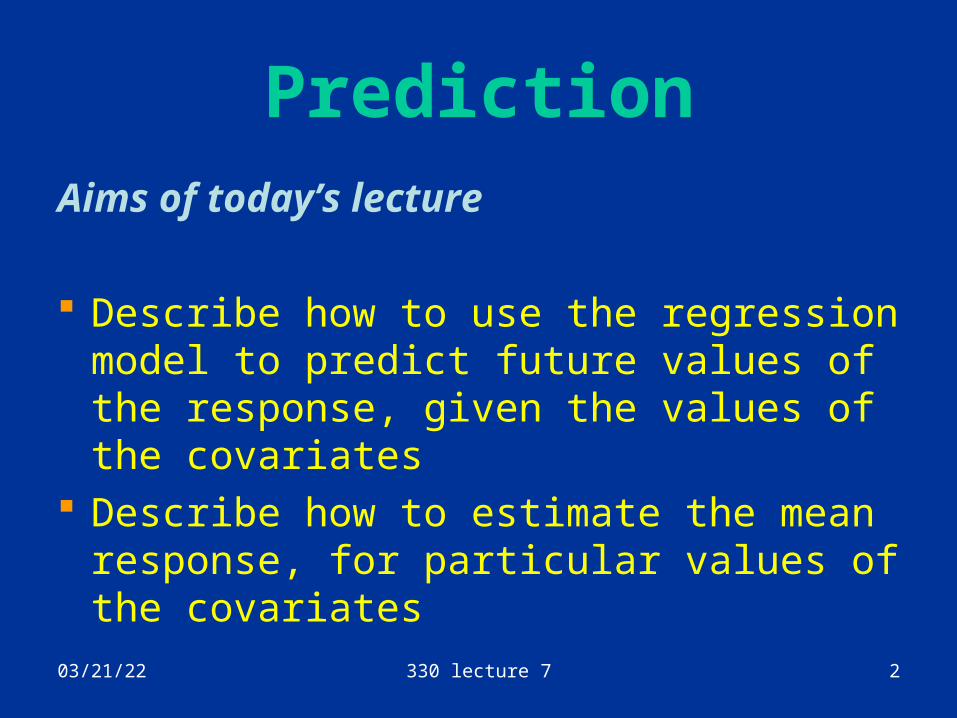
PredictionAims of today’s lecture

Describe how to use the regression model to predict future values of the response, given the values of the covariates

Describe how to estimate the mean response, for particular values of the covariates

04/18/23 330 lecture 7 3

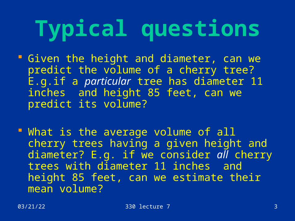
Typical questions Given the height and diameter, can we predict

the volume of a cherry tree? E.g.if a particular tree has diameter 11 inches and height 85 feet, can we predict its volume?

What is the average volume of all cherry trees having a given height and diameter? E.g. if we consider all cherry trees with diameter 11 inches and height 85 feet, can we estimate their mean volume?

04/18/23 330 lecture 7 4

The regression model (revisited)

aaa

Y

X1

O

X2

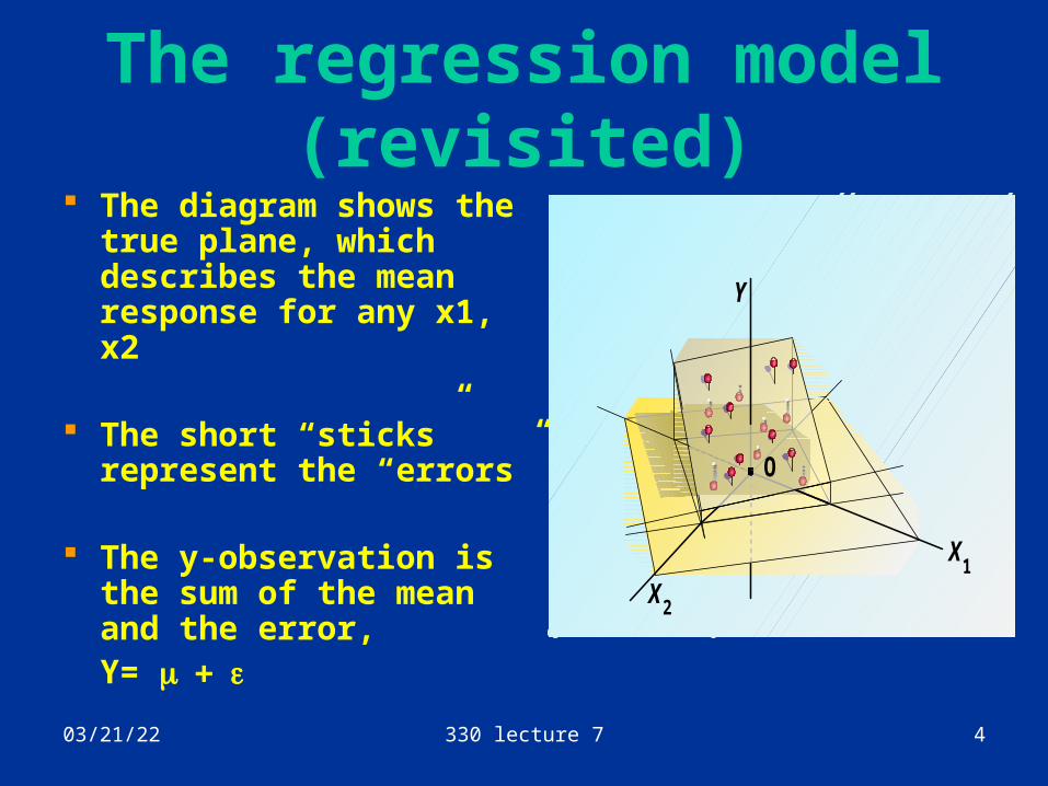
The diagram shows the true plane, which describes the mean response for any x1, x2

The short “sticks”

represent the “errors”

The y-observation is the sum of the mean and the error,Y=

04/18/23 330 lecture 7 5

Prediction: how to do it

Suppose we want to predict the response of an individual whose covariates are

x1, … xk. for the cherry tree example, k=2 and x1

(height) is 85, x2 (diameter) is 11 Since the response we want to predict is

Y= we predict Y by making separate predictions of and and adding the results together.

04/18/23 330 lecture 7 6

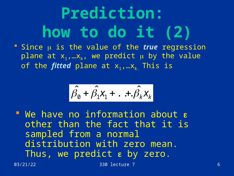
Prediction: how to do it (2)

Since is the value of the true regression plane at x1,…xk, we predict by the value of the fitted plane at x1,…xk. This is

kk xx ˆ...ˆˆ110

We have no information about other than the fact that it is sampled from a normal distribution with zero mean. Thus, we predict by zero.

04/18/23 330 lecture 7 7

Prediction: how to do it (3)

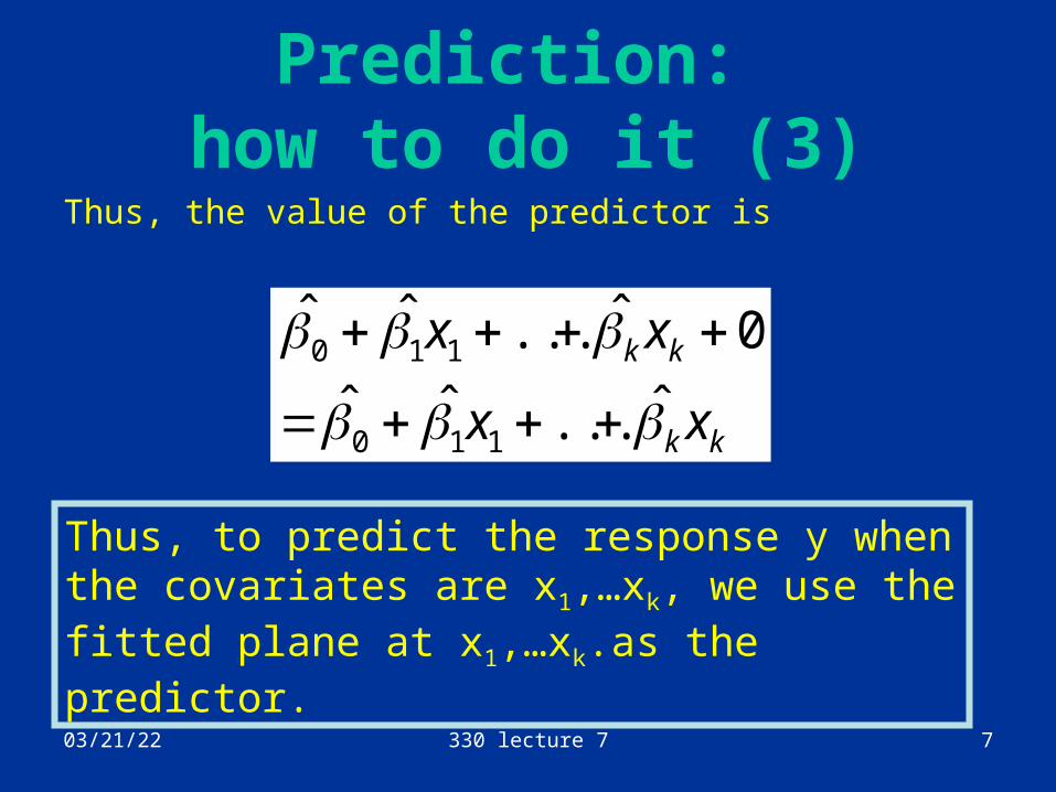
Thus, the value of the predictor is

kk

kk

xx

xx

ˆ...ˆˆ

0ˆ...ˆˆ

110

110

Thus, to predict the response y when the covariates are x1,…xk, we use the fitted plane at x1,…xk.as the predictor.

04/18/23 330 lecture 7 8

Inner product form Inner product form of predictor:

kk

k

k

xxx

xxx

ˆ...ˆˆˆ'

),...,,1(

)ˆ,...,ˆ,ˆ(ˆ

110

1

10

Vector of regression coefficients

Vector of predictor variables

Inner product

04/18/23 330 lecture 7 9

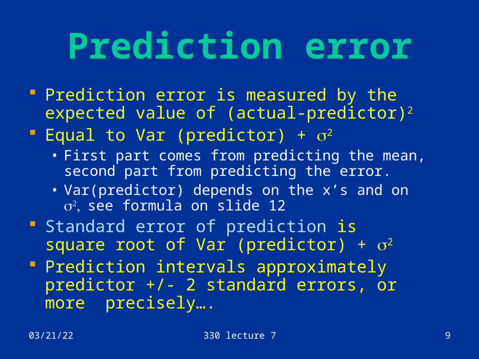
Prediction error Prediction error is measured by the expected

value of (actual-predictor)2

Equal to Var (predictor) + 2

• First part comes from predicting the mean, second part from predicting the error.

• Var(predictor) depends on the x’s and on see formula on slide 12

Standard error of prediction is square root of Var (predictor) + 2

Prediction intervals approximately predictor +/- 2 standard errors, or more precisely….

04/18/23 330 lecture 7 10

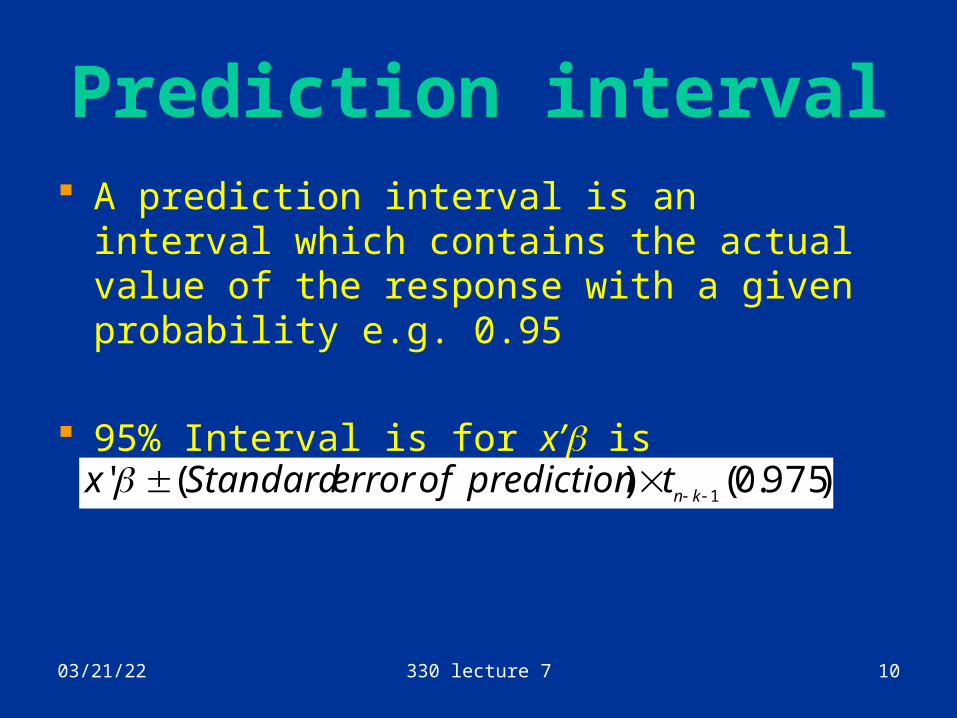
Prediction interval A prediction interval is an interval which

contains the actual value of the response with a given probability e.g. 0.95

95% Interval is for x’ is

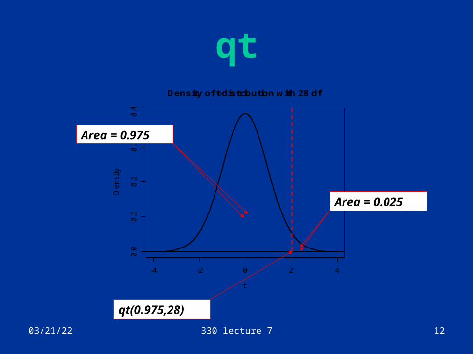
)975.0()('1

kntprediction of error Standardx

04/18/23 330 lecture 7 11

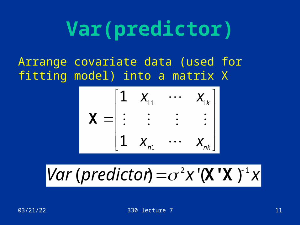
Var(predictor)

Arrange covariate data (used for fitting model) into a matrix X

nkn

k

xx

xx

1

111

1

1

X

xxpredictorVar 12 )(')( XX'

04/18/23 330 lecture 7 12

qt

qt(0.975,28)

-4 -2 0 2 4

0.0

0.1

0.2

0.3

0.4

Density of t-distribution with 28 df

t

De

nsity

Area = 0.975

Area = 0.025

04/18/23 330 lecture 7 13

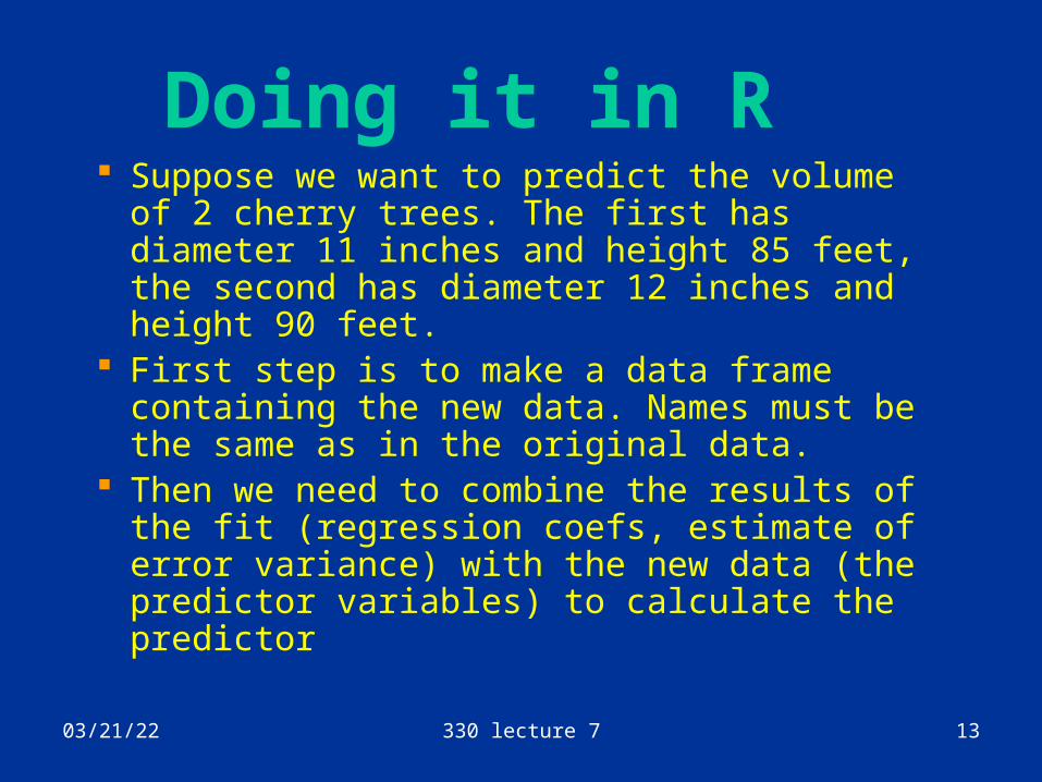
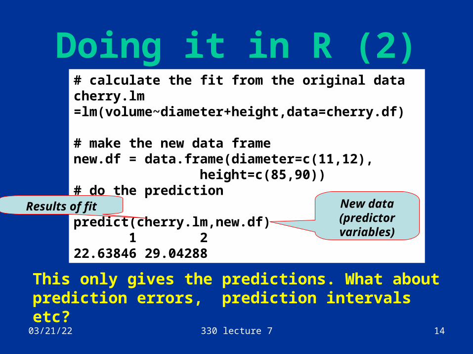
Doing it in R Suppose we want to predict the volume of 2

cherry trees. The first has diameter 11 inches and height 85 feet, the second has diameter 12 inches and height 90 feet.

First step is to make a data frame containing the new data. Names must be the same as in the original data.

Then we need to combine the results of the fit (regression coefs, estimate of error variance) with the new data (the predictor variables) to calculate the predictor

04/18/23 330 lecture 7 14

Doing it in R (2)

This only gives the predictions. What about prediction errors, prediction intervals etc?

# calculate the fit from the original datacherry.lm =lm(volume~diameter+height,data=cherry.df)

# make the new data framenew.df = data.frame(diameter=c(11,12),

height=c(85,90))# do the prediction

predict(cherry.lm,new.df) 1 2 22.63846 29.04288

New data (predictor variables)

Results of fit

04/18/23 330 lecture 7 15

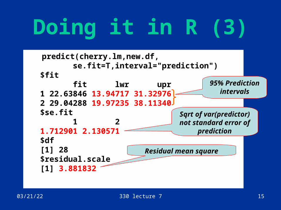
predict(cherry.lm,new.df, se.fit=T,interval="prediction")$fit fit lwr upr1 22.63846 13.94717 31.329762 29.04288 19.97235 38.11340$se.fit 1 2 1.712901 2.130571 $df[1] 28$residual.scale[1] 3.881832

Doing it in R (3)

95% Prediction intervals

Sqrt of var(predictor) not standard error of

prediction

Residual mean square

04/18/23 330 lecture 7 16

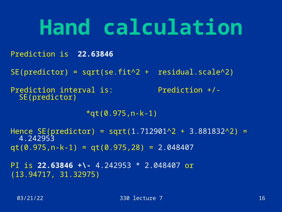
Hand calculationPrediction is 22.63846

SE(predictor) = sqrt(se.fit^2 + residual.scale^2)

Prediction interval is: Prediction +/- SE(predictor) *qt(0.975,n-k-1)

Hence SE(predictor) = sqrt(1.712901^2 + 3.881832^2) = 4.242953qt(0.975,n-k-1) = qt(0.975,28) = 2.048407

PI is 22.63846 +\- 4.242953 * 2.048407 or(13.94717, 31.32975)

04/18/23 330 lecture 7 17

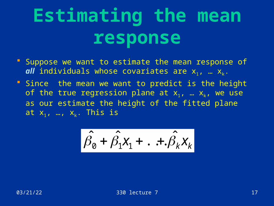
Estimating the mean response

Suppose we want to estimate the mean response of all individuals whose covariates are x1, … xk.

Since the mean we want to predict is the height of the true regression plane at x1, … xk, we use as our estimate the height of the fitted plane at x1, …, xk. This is

kk xx ˆ...ˆˆ110

04/18/23 330 lecture 7 18

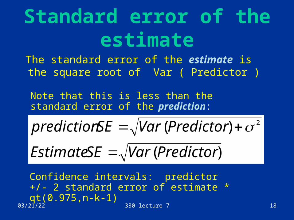
Standard error of the estimate

The standard error of the estimate is the square root of Var ( Predictor )

)(

)( 2

PredictorVarSE Estimate

PredictorVarSE prediction

Note that this is less than the standard error of the prediction:

Confidence intervals: predictor +/- 2 standard error of estimate * qt(0.975,n-k-1)

04/18/23 330 lecture 7 19

Doing it in R Suppose we want to estimate the

mean volume of all cherry trees having diameter 11 inches and height 85 feet.

As before, the first step is to make a data frame containing the new data. Names must be the same as in the original data.

04/18/23 330 lecture 7 20

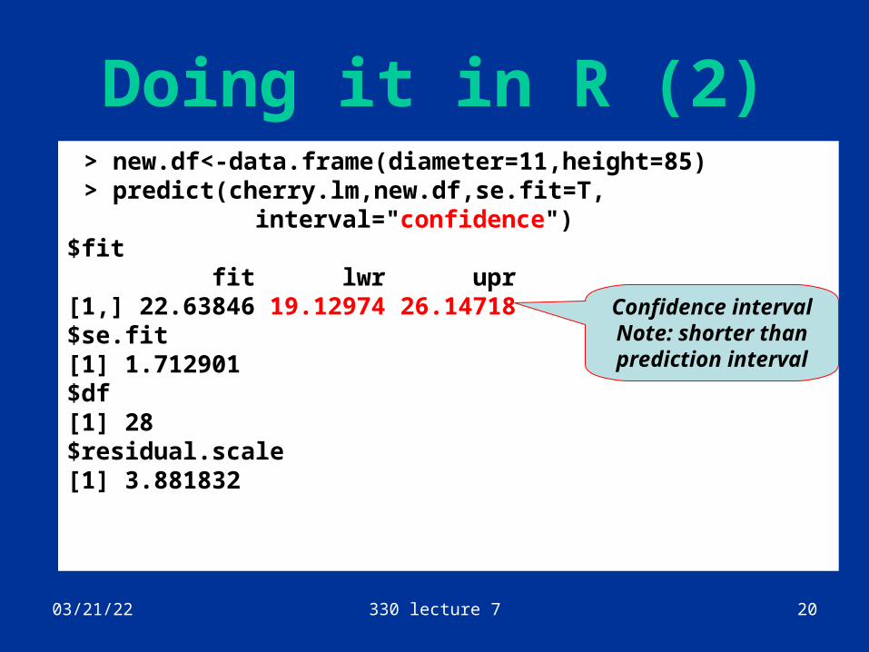
> new.df<-data.frame(diameter=11,height=85)> predict(cherry.lm,new.df,se.fit=T,

interval="confidence")$fit fit lwr upr[1,] 22.63846 19.12974 26.14718$se.fit[1] 1.712901$df[1] 28$residual.scale[1] 3.881832

Doing it in R (2)

Confidence intervalNote: shorter than prediction interval

04/18/23 330 lecture 7 21

Example: Hydrocarbon data

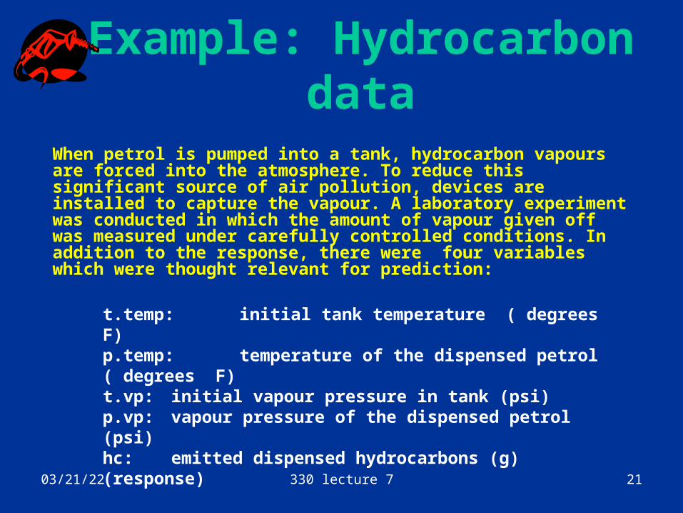
When petrol is pumped into a tank, hydrocarbon vapours are forced into the atmosphere. To reduce this significant source of air pollution, devices are installed to capture the vapour. A laboratory experiment was conducted in which the amount of vapour given off was measured under carefully controlled conditions. In addition to the response, there were four variables which were thought relevant for prediction:

t.temp: initial tank temperature ( degrees F)p.temp: temperature of the dispensed petrol ( degrees F)t.vp: initial vapour pressure in tank (psi)p.vp: vapour pressure of the dispensed petrol (psi)hc: emitted dispensed hydrocarbons (g) (response)

04/18/23 330 lecture 7 22

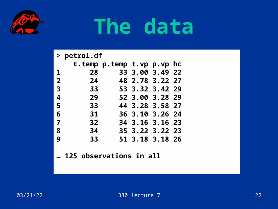
The data> petrol.df t.temp p.temp t.vp p.vp hc1 28 33 3.00 3.49 222 24 48 2.78 3.22 273 33 53 3.32 3.42 294 29 52 3.00 3.28 295 33 44 3.28 3.58 276 31 36 3.10 3.26 247 32 34 3.16 3.16 238 34 35 3.22 3.22 239 33 51 3.18 3.18 26

… 125 observations in all

04/18/23 330 lecture 7 23

Pairs plot

t.temp

40 60 80 3 4 5 6 7

30

50

70

90

40

60

80

p.temp

t.vp

34

56

7

34

56

7

p.vp

30 50 70 90 3 4 5 6 7 20 30 40 50

20

30

40

50

hc

04/18/23 330 lecture 7 24

Preliminary conclusion

All variables seem related to the response p.vp and t.vp seem highly correlated Quite strong correlations between some of

the other variables No obvious outliers

04/18/23 330 lecture 7 25

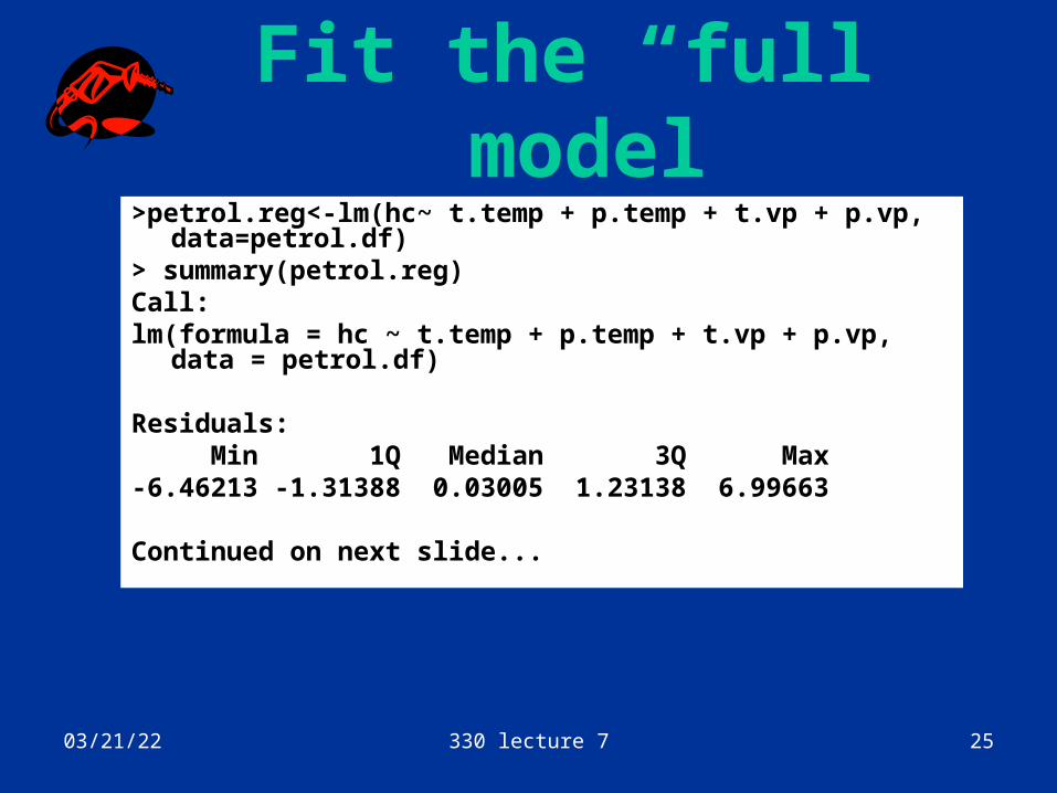
Fit the “full” model

>petrol.reg<-lm(hc~ t.temp + p.temp + t.vp + p.vp, data=petrol.df)

> summary(petrol.reg)Call:lm(formula = hc ~ t.temp + p.temp + t.vp + p.vp,

data = petrol.df)

Residuals: Min 1Q Median 3Q Max -6.46213 -1.31388 0.03005 1.23138 6.99663

Continued on next slide...

04/18/23 330 lecture 7 26

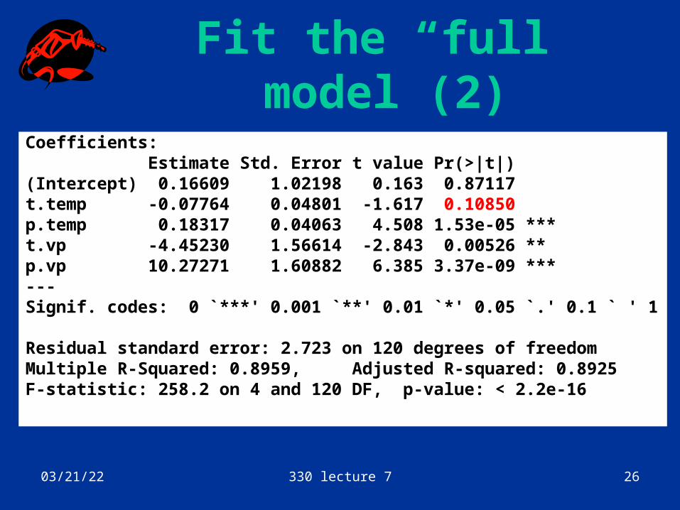
Fit the “full” model (2)

Coefficients: Estimate Std. Error t value Pr(>|t|) (Intercept) 0.16609 1.02198 0.163 0.87117 t.temp -0.07764 0.04801 -1.617 0.10850 p.temp 0.18317 0.04063 4.508 1.53e-05 ***t.vp -4.45230 1.56614 -2.843 0.00526 ** p.vp 10.27271 1.60882 6.385 3.37e-09 ***---Signif. codes: 0 `***' 0.001 `**' 0.01 `*' 0.05 `.' 0.1 ` ' 1

Residual standard error: 2.723 on 120 degrees of freedomMultiple R-Squared: 0.8959, Adjusted R-squared: 0.8925 F-statistic: 258.2 on 4 and 120 DF, p-value: < 2.2e-16

04/18/23 330 lecture 7 27

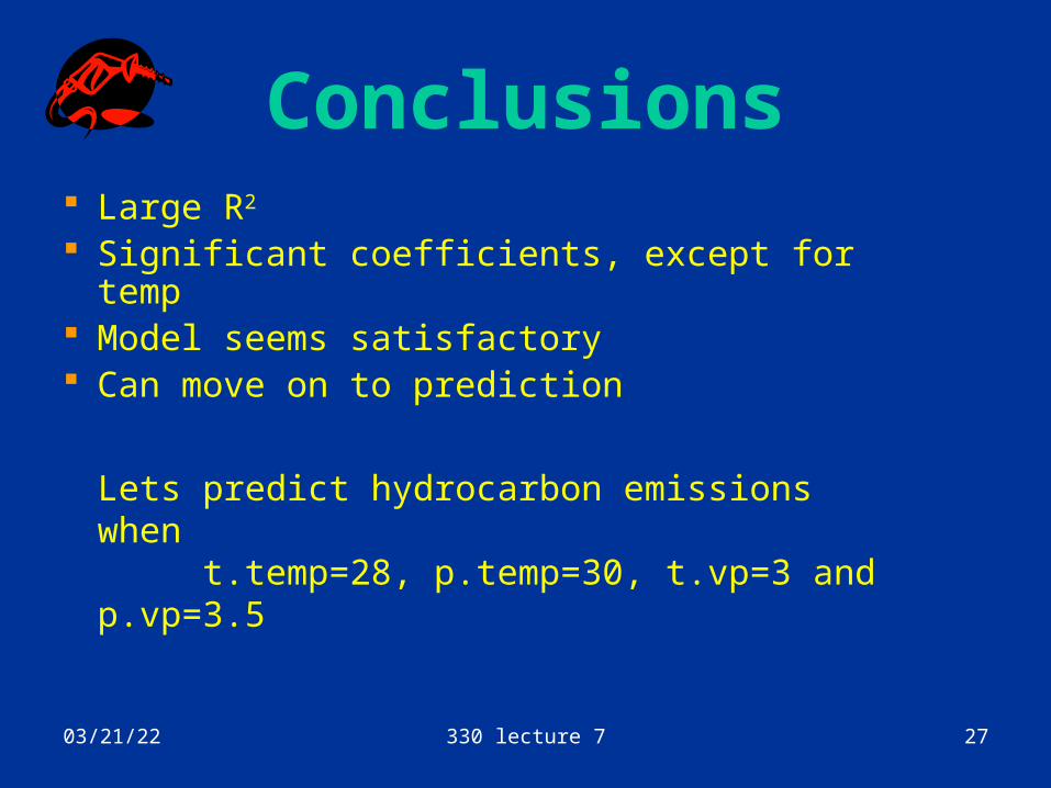
Conclusions Large R2

Significant coefficients, except for temp Model seems satisfactory Can move on to prediction

Lets predict hydrocarbon emissions whent.temp=28, p.temp=30, t.vp=3 and p.vp=3.5

04/18/23 330 lecture 7 28

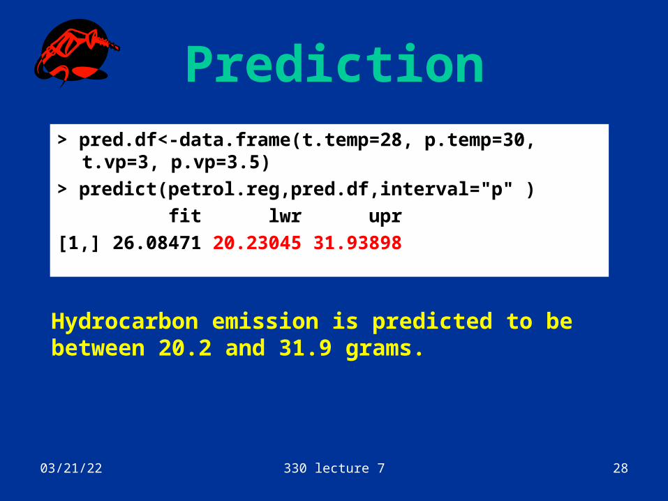
Prediction> pred.df<-data.frame(t.temp=28, p.temp=30,

t.vp=3, p.vp=3.5)

> predict(petrol.reg,pred.df,interval="p" )

fit lwr upr

[1,] 26.08471 20.23045 31.93898

Hydrocarbon emission is predicted to be between 20.2 and 31.9 grams.