5.1 influence of demographic factors on …shodhganga.inflibnet.ac.in/bitstream/10603/40636/8/v...
TRANSCRIPT

160
5.1 INFLUENCE OF DEMOGRAPHIC FACTORS ON BUYING
PATTERN OF RURAL CONSUMERS
This chapter discusses the influence of demographic factors on buying pattern
of rural consumers. The demographic characteristics taken up for the study of gender,
age group, educational qualification, marital status, occupation and family income of
the respondents. The inferential statistics of the respondents based on each of the
above demographic variables are given in this chapter.
HYPOTHESIS 1
There is no significant association between demographic factors (Gender,
Age, Educational Qualification, Marital Status, Occupation and Family Income) of
the respondents and their Need Recognition stage of consumer durable goods (CTV,
Refrigerator, Fan, Mixie and Grinder).
5.1.1. INFLUENCE OF DEMOGRAPHIC FACTORS IN THE NEED
RECOGNITION BUYING PATTERN OF RESPONDENTS
Ho: there is no significant association between demographic factors of the
respondents and their Need Recognition for CTV.
To test the above hypothesis Chi Square Analysis is used.

161
Table No. 5.1Association between Demographic Factors of the respondents and their Need
Recognition for CTV
DemographicFactors
Need Recognition for CTV Statistical Inference
More % Less % Total %Chi-
SquareValue
P Value
GenderMale 109 64.90 122 65.60 231 65.30
0.20 0.889**Female 59 35.10 64 34.40 123 34.70Total 168 186 354AgeLess than 20 years 8 4.80 13 7.00 25 5.90
0.835 0.841**21 – 40 years 84 50.00 92 49.50 176 49.7041 – 60 Years 62 36.90 67 36.00 129 36.4061 years & More 14 8.30 14 7.50 28 7.90Total 168 186 354EducationalQualificationSSLC
32 19.00 25 13.40 57 16.10
3.286 0.511**HSC 38 22.60 36 19.40 74 20.90UG 40 23.80 51 27.40 91 25.70PG 42 25.00 53 28.50 95 26.80Others 16 9.50 21 11.30 37 10.50Total 168 186 354Marital StatusMarried 153 91.10 160 86.00 313 88.40
2.198 0.138**Unmarried 15 8.90 26 14.00 41 11.60Total 168 186 354OccupationEmployee in PrivateServices
37 22.00 45 24.20 82 23.20
0.908 0.970**
Business/Profession 34 20.20 35 18.80 69 19.50Employee in Govt.Services 14 8.30 17 9.10 31 8.80
Agriculture 54 32.10 60 32.30 114 32.20Housewife 24 14.30 22 11.80 46 13.00Others 5 3.00 7 3.80 12 3.40Total 168 186 354Family IncomeBelow Rs. 5000 5 3.00 3 1.60 8 2.30
2.080 0.838**
Rs. 5000 – 10000 45 26.80 46 24.70 91 25.70Rs. 10001 -15000 31 18.50 34 18.30 65 18.40Rs. 15001 – 20000 31 18.50 38 20.40 69 19.50Rs. 20001 – 25000 30 17.90 29 15.60 59 16.70Rs. 25001 & above 26 15.50 36 19.40 62 17.50Total 168 186 354
* Significant ** Not Significant

162
The above table clearly shown that there is no significant association between
gender, age, educational qualification, marital status, occupation, family income of
the respondents and their need recognition for CTV. Hence Hypothesis (H0) is
accepted. Further it is observed that the need recognition is more or less same among
the demographic factors of the respondents.
Ho: There is no significant association between demographic factors of the
respondents and their Need Recognition for Refrigerator.
To test the above hypothesis Chi Square Analysis is used.
Table No. 5.2
Association between Demographic Factors of the respondents and their
Need Recognition for Refrigerator
DemographicFactors
Need Recognition for Refrigerator StatisticalInference
More % Less % Total %Chi-
SquareValue
PValue
GenderMale 111 65.30 121 65.40 232 65.40
0.003 0.953**Female 59 34.70 64 34.60 123 34.60Total 170 185 355AgeLess than 20 years 8 4.70 13 7.00 21 5.90
1.076 0.783**21 – 40 years 81 47.60 86 46.50 167 47.0041 – 60 Years 70 41.20 72 38.90 142 40.1061 years & More 11 6.50 14 7.60 25 7.00Total 170 185 355EducationalQualificationSSLC
3319.40
2815.10
6117.20
2.216 0.696**HSC 41 24.10 39 21.00 80 22.50UG 37 21.80 46 24.90 83 23.40PG 44 25.90 54 29.20 98 27.60Others 15 8.80 18 9.80 33 9.30Total 170 185 355Marital StatusMarried 157 92.40 162 87.60 319 89.90
2.635 0.105**Unmarried 13 7.60 23 12.40 36 10.10Total 170 100.00 185 100.00 355 100.00

163
DemographicFactor
Need Recognition for Refrigerator StatisticalInference
More % Less % Total %Chi-
SquareValue
PValue
OccupationEmployee inPrivate Services
41 24.10 49 26.50 90 25.40
1.532 0.909**
Business /Profession 31 18.20 30 16.20 61 17.20
Employee in Govt.Services 14 8.20 17 9.20 31 8.70
Agriculture 54 31.80 58 31.30 112 31.50Housewife 24 14.10 22 11.90 46 13.00Others 6 3.50 9 4.90 15 4.20Total 170 185 355Family IncomeBelow Rs. 5000 5 2.90 3 1.60 8 2.20
2.216 0.819**
Rs. 5000 – 10000 47 27.60 48 25.90 95 26.80Rs. 10001 -15000 32 18.80 30 16.20 62 17.50Rs. 15001 – 20000 33 19.40 40 21.60 73 20.50Rs. 20001 – 25000 27 15.90 29 15.70 56 15.80Rs. 25001 & above 26 15.30 35 19.00 61 17.20Total 170 100.00 185 100.00 355 100.00
*Significant ** Not Significant
It is observed from the above table that there is no significant association
between gender, age, educational qualification, marital status, occupation, family
income of the respondents and their need recognition for refrigerator. Hence
Hypothesis (H0) is accepted. Further it is observed that the need recognition is more
or less same among the demographic factors of the respondents.
Ho: There is no significant association between demographic factors of the
respondents and their Need Recognition for Fan.
To test the above hypothesis Chi Square Analysis is used.

164
Table No. 5.3Association between Demographic Factors of the respondents and their
Need Recognition for Fan
DemographicFactors
Need Recognition for Fan StatisticalInference
More % Less % Total %Chi-
SquareValue
PValue
GenderMale 117 66.10 131 66.20 248 66.10
0.005 0.990**Female 60 33.90 67 33.80 127 33.90Total 177 198 375Age Less than 20years 10 5.60 15 7.60 25 6.70
0.982 0.806**21 – 40 years 85 48.00 95 48.00 180 48.0041 – 60 Years 70 39.50 72 36.40 142 37.9061 years & More 12 6.80 16 8.10 28 7.50Total 177 198 375EducationalQualificationSSLC
33 18.60 28 14.10 61 16.30
2.498 0.645**HSC 42 23.70 41 20.70 83 22.10UG 41 23.20 54 27.30 95 25.30PG 44 24.90 55 27.80 99 26.40Others 17 9.60 20 10.10 37 9.90Total 177 198 375Marital StatusMarried 161 91.00 169 85.40 330 88.00
2.782 0.095**Unmarried 16 9.00 29 14.60 45 12.00Total 177 198 375OccupationEmployee in PrivateServices
442 23.70 52 26.30 94 25.10
1.494 0.914**
Business /Profession 34 19.20 35 17.70 69 18.40
Employee in Govt.Services 14 7.90 17 8.60 31 8.30
Agriculture 57 32.20 62 31.30 119 31.70Housewife 24 13.60 22 11.10 46 12.30Others 6 3.40 10 5.10 16 4.30Total 177 198 375Family IncomeBelow Rs. 5000 5 2.80 3 1.50 8 2.10
1.854 0.869**
Rs. 5000 – 10000 50 28.20 53 26.80 103 27.50Rs. 10001 -15000 35 19.80 35 17.70 70 18.70Rs. 15001 – 20000 33 18.60 40 20.20 73 19.50Rs. 20001 – 25000 28 15.80 31 15.70 59 15.70Rs. 25001 & above 26 14.70 36 18.20 62 16.50Total 177 198 375
*Significant ** Not Significant

165
It is seen from the above table that there is no significant association between
gender, age, educational qualification, marital status, occupation, family income of
the respondents and their need recognition for fan. Hence Hypothesis (H0) is
accepted. Further it is observed that the need recognition is more or less same among
the demographic factors of the respondents.
Ho: There is no significant association between demographic factors of the
respondents and their Need Recognition for Mixie.
To test the above hypothesis Chi Square Analysis is used.
Table No. 5.4
Association between Demographic Factors of the respondents and their
Need Recognition for Mixie
DemographicFactors
Need Recognition for Mixie StatisticalInference
More % Less % Total %Chi-
SquareValue
P Value
GenderMale 117 66.10 131 66.20 248 66.10
0.005 0.990**Female 60 33.90 67 33.80 127 33.90Total 177 198 375AgeLess than 20 years 10 5.60 15 7.60 25 6.70
0.982 0.806**21 – 40 years 85 48.00 95 48.00 180 48.0041 – 60 Years 70 39.50 72 36.40 142 37.9061 years & More 12 6.80 16 8.10 28 7.50Total 177 198 375EducationalQualificationSSLC
33 18.60 28 14.10 61 16.30
2.498 0.645**HSC 42 23.70 41 20.70 83 22.10UG 41 23.20 54 27.30 95 25.30PG 44 24.90 55 27.80 99 26.40
Others 17 9.60 20 10.10 37 9.90Total 177 198 375Marital StatusMarried 161 91.00 169 85.40 330 88.00
2.782 0.095**Unmarried 16 9.00 29 14.60 45 12.00Total 177 198 375

166
DemographicFactors
Need Recognition for Mixie StatisticalInferenceMore % Less % Total %
OccupationEmployee inPrivate Services
42 23.70 52 26.30 94 25.10
1.494 0.914**
Business /Profession 34 19.20 35 17.70 69 18.40
Employee in Govt.Services 14 7.90 17 8.60 31 8.30
Agriculture 57 32.20 62 31.30 119 31.70Housewife 24 13.60 22 11.10 46 12.30Others 6 3.40 10 5.10 16 4.30Total 177 198 375Family IncomeBelow Rs. 5000 5 2.80 3 1.50 8 2.10
1.854 0.869**
Rs. 5000 – 10000 50 28.20 53 26.80 103 27.50Rs. 10001 -15000 35 19.80 35 17.70 70 18.70Rs. 15001 – 20000 33 18.60 40 20.20 73 19.50Rs. 20001 – 25000 28 15.80 31 15.70 59 15.70Rs. 25001 & above 26 14.70 36 18.20 62 16.50Total 177 198 375
*Significant ** Not Significant
The above table indicates that there is no significant association between
gender, age, educational qualification, marital status, occupation, family income of
the respondents and their need recognition for mixie. Hence Hypothesis (H0) is
accepted. Further it is observed that the need recognition is more or less same among
the demographic factors of the respondents.
Ho: There is no significant association between demographic factors of the
respondents and their Need Recognition for Grinder.
To test the above hypothesis Chi Square Analysis is used.

167
Table No. 5.5
Association between Demographic Factors of the respondents and their
Need Recognition for Grinder
DemographicFactors
Need Recognition for Grinder StatisticalInference
More % Less % Total %Chi-
SquareValue
P Value
GenderMale 117 66.10 131 66.20 248 66.10
0.125 0.990**Female 60 33.90 67 33.80 127 33.90Total 177 198 375AgeLess than 20 years 10 5.60 15 7.60 25 6.70
0.982 0.806**21 – 40 years 85 48.00 95 48.00 180 48.0041 – 60 Years 70 39.50 72 36.40 142 37.9061 years & More 12 6.80 16 8.10 28 7.50Total 177 198 375EducationalQualificationSSLC
33 18.60 28 14.10 61 16.30
2.498 0.645**HSC 42 23.70 41 20.70 83 22.10UG 41 23.20 54 27.30 95 25.30PG 44 24.90 55 27.80 99 26.40
Others 17 9.60 20 10.10 37 9.90Total 177 198 375Marital StatusMarried 161 91.00 169 85.40 330 88.00
2.782 0.095**Unmarried 16 9.00 29 14.60 45 12.00Total 177 198 375OccupationEmployee in PrivateServices
42 23.70 52 26.30 94 25.10
1.494 0.914**
Business /Profession 34 19.20 35 17.70 69 18.44
Employee in Govt.Services 14 7.90 17 8.60 31 8.30
Agriculture 57 32.20 62 31.30 119 31.70Housewife 24 13.60 22 11.10 46 12.30Others 6 3.40 10 5.10 16 4.30Total 177 198 375Family IncomeBelow Rs. 5000 5 2.80 3 1.50 8 2.10
1.854 0.869**Rs. 5000 – 10000 50 28.20 53 26.80 103 27.50Rs. 10001 -15000 35 19.80 35 17.70 70 18.70Rs. 15001 – 20000 33 18.60 40 20.20 73 19.50Rs. 20001 – 25000 28 18.80 31 15.70 59 15.70Rs. 25001 & above 26 14.70 36 18.20 62 16.50Total 177 198 375
*Significant ** Not Significant

168
It is observed from the above table that there is no significant association
between gender, age, educational qualification, marital status, occupation, family
income of the respondents and their need recognition for grinder. Hence Hypothesis
(H0) is accepted. Further it is observed that the need recognition is more or less same
among the demographic factors of the respondents.
HYPOTHESIS 2
There is no significant association between demographic factors (Gender,
Age, Educational Qualification, Marital Status, Occupation and Family Income) of
the respondents and their Information Search stage of consumer durable goods (CTV,
Refrigerator, Fan, Mixie and Grinder)
5.1.2. INFLUENCE OF DEMOGRAPHIC FACTORS IN THE INFORMATION
SEARCH OF RESPONDENTS
Ho: there is no significant association between demographic factors of the
respondents and their Information Search for CTV.
To test the above hypothesis Chi Square Analysis is used.

169
Table No. 5.6Association between Demographic Factors of the respondents and their
Information Search for CTV
DemographicFactors
Information Search for CTV StatisticalInference
MoreInclined % Less
Inclined % Total %Chi-
SquareValue
PValue
GenderMale 183 66.80 48 60.00 231 65.30
1.258 0.262**Female 91 33.20 32 40.00 123 34.70Total 274 80 354AgeLess than 20 years 13 4.70 8 10.00 21 5.90
4.050 0.256**21 – 40 years 136 49.60 40 50.00 176 49.7041 – 60 Years 101 36.90 28 35.00 129 36.4061 years & More 24 8.80 4 5.00 28 7.90Total 274 84 354EducationalQualificationSSLC
45 16.40 12 15.00 57 16.10
9.649 0.047*HSC 50 18.20 24 33.30 78 21.10UG 71 24.80 24 30.00 74 20.90PG 79 28.80 16 20.00 95 26.80Others 33 12.00 4 5.00 37 10.50Total 274 80 354Marital StatusMarried 237 86.50 76 95.00 313 88.40
4.372 0.037*Unmarried 37 13.50 4 5.00 41 11.60Total 274 80 354OccupationEmployee in PrivateServices
70 25.50 12 15.00 82 23.20
21.861 0.001**
Business/Profession 41 15.00 28 35.00 69 19.50Employee in Govt.Services 27 9.90 4 5.00 31 8.80
Agriculture 86 31.40 28 35.00 114 32.20Housewife 38 13.90 8 10.00 46 13.00Others 12 4.40 0 0.00 12 3.40Total 274 80 354Family IncomeBelow Rs. 5000 4 1.50 4 5.00 8 2.30
31.092 0.001**
Rs. 5000 – 10000 67 24.50 24 30.00 91 25.70Rs. 10001 -15000 41 15.00 24 30.00 65 18.40Rs. 15001 – 20000 49 17.90 20 25.00 69 19.50Rs. 20001 – 25000 55 20.10 4 5.00 59 16.70Rs. 25001 & above 58 21.20 4 5.00 62 17.50Total 274 80 354
*Significant ** Not Significant
170
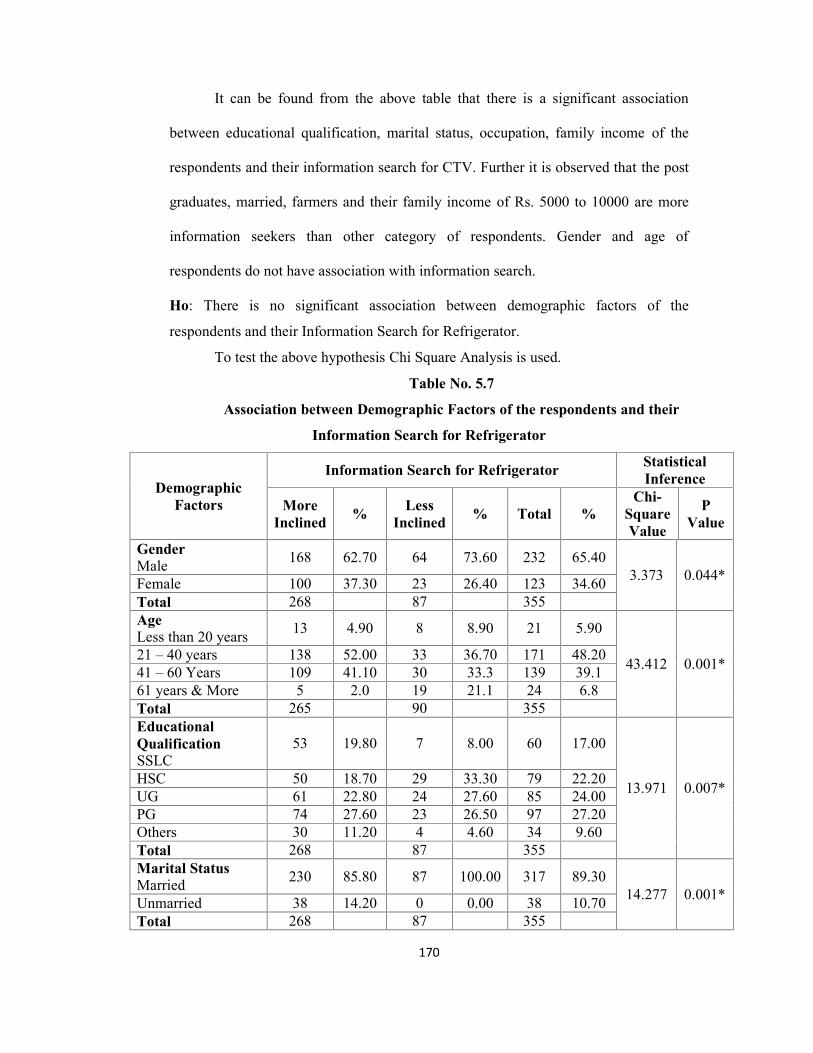
It can be found from the above table that there is a significant association
between educational qualification, marital status, occupation, family income of the
respondents and their information search for CTV. Further it is observed that the post
graduates, married, farmers and their family income of Rs. 5000 to 10000 are more
information seekers than other category of respondents. Gender and age of
respondents do not have association with information search.
Ho: There is no significant association between demographic factors of the
respondents and their Information Search for Refrigerator.
To test the above hypothesis Chi Square Analysis is used.
Table No. 5.7
Association between Demographic Factors of the respondents and their
Information Search for Refrigerator
DemographicFactors
Information Search for Refrigerator StatisticalInference
MoreInclined % Less
Inclined % Total %Chi-
SquareValue
PValue
GenderMale 168 62.70 64 73.60 232 65.40
3.373 0.044*Female 100 37.30 23 26.40 123 34.60Total 268 87 355AgeLess than 20 years 13 4.90 8 8.90 21 5.90
43.412 0.001*21 – 40 years 138 52.00 33 36.70 171 48.2041 – 60 Years 109 41.10 30 33.3 139 39.161 years & More 5 2.0 19 21.1 24 6.8Total 265 90 355EducationalQualificationSSLC
53 19.80 7 8.00 60 17.00
13.971 0.007*HSC 50 18.70 29 33.30 79 22.20UG 61 22.80 24 27.60 85 24.00PG 74 27.60 23 26.50 97 27.20Others 30 11.20 4 4.60 34 9.60Total 268 87 355Marital StatusMarried 230 85.80 87 100.00 317 89.30
14.277 0.001*Unmarried 38 14.20 0 0.00 38 10.70Total 268 87 355

171
DemographicFactor
Information Search for Refrigerator StatisticalInference
MoreInclined % Less
Inclined % Total %Chi
SquareValue
PValue
OccupationEmployee in PrivateServices
74 27.60 17 19.50 91 25.60
26.185 0.001*
Business/Profession 38 14.20 22 25.30 60 16.90Employee in Govt.Services 18 6.70 13 15.00 31 8.70
Agriculture 80 29.90 31 35.60 111 31.30Housewife 42 15.70 4 4.60 46 13.00Others 16 6.00 0 0.00 16 4.50Total 268 87 355Family IncomeBelow Rs. 5000 8 3.00 0 0.00 8 2.20
51.713 0.001*
Rs. 5000 – 10000 92 34.30 4 4.60 96 27.00Rs. 10001 -15000 35 13.10 29 33.30 64 18.00Rs. 15001 – 20000 42 15.70 30 34.50 72 20.30Rs. 20001 – 25000 41 15.30 14 16.10 55 15.50Rs. 25001 & above 50 18.70 10 11.50 60 17.00Total 268 87 355
*Significant ** Not Significant
It can be seen from the above table that there is a significant association
between gender, age, educational qualification, marital status, occupation, family
income of the respondents and their information search for refrigerator. Further it is
observed that male, age group of 21 to 40 years, post graduates, married, farmers and
their family income of Rs. 5000 to 10000 are more information seekers than other
category of respondents.
Ho: There is no significant association between demographic factors of the
respondents and their Information Search for Fan.
To test the above hypothesis Chi Square Analysis is used.
172
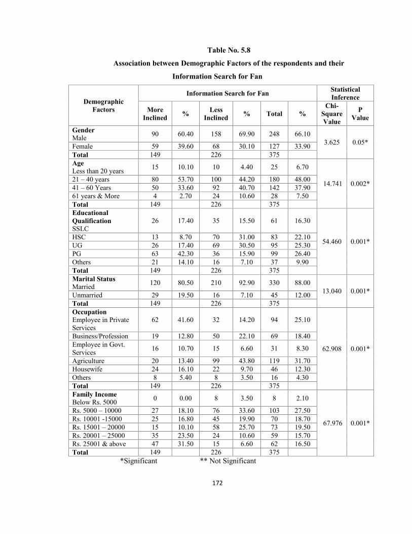
Table No. 5.8
Association between Demographic Factors of the respondents and their
Information Search for Fan
DemographicFactors
Information Search for Fan StatisticalInference
MoreInclined % Less
Inclined % Total %Chi-
SquareValue
PValue
GenderMale 90 60.40 158 69.90 248 66.10
3.625 0.05*Female 59 39.60 68 30.10 127 33.90Total 149 226 375AgeLess than 20 years 15 10.10 10 4.40 25 6.70
14.741 0.002*21 – 40 years 80 53.70 100 44.20 180 48.0041 – 60 Years 50 33.60 92 40.70 142 37.9061 years & More 4 2.70 24 10.60 28 7.50Total 149 226 375EducationalQualificationSSLC
26 17.40 35 15.50 61 16.30
54.460 0.001*HSC 13 8.70 70 31.00 83 22.10UG 26 17.40 69 30.50 95 25.30PG 63 42.30 36 15.90 99 26.40Others 21 14.10 16 7.10 37 9.90Total 149 226 375Marital StatusMarried 120 80.50 210 92.90 330 88.00
13.040 0.001*Unmarried 29 19.50 16 7.10 45 12.00Total 149 226 375OccupationEmployee in PrivateServices
62 41.60 32 14.20 94 25.10
62.908 0.001*
Business/Profession 19 12.80 50 22.10 69 18.40Employee in Govt.Services 16 10.70 15 6.60 31 8.30
Agriculture 20 13.40 99 43.80 119 31.70Housewife 24 16.10 22 9.70 46 12.30Others 8 5.40 8 3.50 16 4.30Total 149 226 375Family IncomeBelow Rs. 5000 0 0.00 8 3.50 8 2.10
67.976 0.001*
Rs. 5000 – 10000 27 18.10 76 33.60 103 27.50Rs. 10001 -15000 25 16.80 45 19.90 70 18.70Rs. 15001 – 20000 15 10.10 58 25.70 73 19.50Rs. 20001 – 25000 35 23.50 24 10.60 59 15.70Rs. 25001 & above 47 31.50 15 6.60 62 16.50Total 149 226 375
*Significant ** Not Significant

173
It is observed from the above table that there is a significant association
between gender, age, educational qualification, marital status, occupation, family
income of the respondents and their information search for fan. Further it is observed
that male, age group for 21 to 40 years, post graduates, married, farmers and their
family income of Rs. 5000 to 10000 are more information seekers than other category
of respondents.
Ho: There is no significant association between demographic factors of the
respondents and their Information Search for Mixie.
To test the above hypothesis Chi Square Analysis is used.
Table No. 5.9
Association between Demographic Factors of the respondents and their
Information Search for Mixie
DemographicFactors
Information Search for Mixie StatisticalInference
MoreInclined % Less
Inclined % Total %Chi-
SquareValue
PValue
GenderMale 126 68.10 122 64.20 248 66.10
0.636 0.425**Female 59 31.90 68 35.80 127 33.90Total 185 190 375AgeLess than 20 years 8 4.30 17 8.90 25 6.70
16.317 0.001*21 – 40 years 75 40.50 105 55.30 180 48.0041 – 60 Years 88 47.60 54 28.40 142 37.9061 years & More 14 7.60 14 7.40 28 7.50Total 185 190 375EducationalQualificationSSLC
35 18.90 26 13.70 61 16.30
16.244 0.003*HSC 51 27.60 32 16.80 83 22.10UG 49 26.50 46 24.20 95 25.30PG 39 21.10 60 31.60 99 26.40Others 11 5.90 26 13.70 37 9.90Total 185 190 375Marital StatusMarried 177 95.70 153 80.50 330 88.00
20.371 0.001*Unmarried 8 4.30 37 19.50 45 12.00Total 185 190 375

174
DemographicFactors
Information Search for Mixie StatisticalInference
MoreInclined % Less
Inclined % Total %Chi-
SquareValue
PValue
OccupationEmployee in Private
Services29 15.70 65 34.20 94 25.10
37.248 0.001*
Business/Profession 47 25.40 22 11.60 69 18.40Employee in Govt.
Services 11 5.90 20 10.50 31 8.30
Agriculture 74 40.00 45 23.70 119 31.70Housewife 20 10.80 26 13.70 46 12.30
Others 4 2.20 12 6.30 16 4.30Total 185 190 375
Family IncomeBelow Rs. 5000 4 2.20 4 2.10 8 2.10
22.473 0.001*
Rs. 5000 – 10000 58 31.40 45 23.70 103 27.50Rs. 10001 -15000 43 23.20 27 14.20 70 18.70
Rs. 15001 – 20000 40 21.60 33 17.40 73 19.50Rs. 20001 – 25000 24 13.00 35 18.40 59 15.70Rs. 25001 & above 16 8.60 46 24.20 62 16.50
Total 185 190 375*Significant ** Not Significant
The above table clearly shown that there is a significant association between
age, educational qualification, marital status, occupation, family income of the
respondents and their information search for mixie. Further it is observed that age
group for 21 to 40 years, post graduates, married, farmers and their family income of
Rs. 5000 to 10000 are more information seekers than other category of respondents.
Genders of respondents do not have association with information search.
Ho: There is no significant association between demographic factors of the
respondents and their Information Search for Grinder.
To test the above hypothesis Chi Square Analysis is used.

175
Table No. 5.10Association between Demographic Factors of the respondents and their
Information Search for Grinder
DemographicFactors
Information Search for Grinder StatisticalInference
MoreInclined % Less
Inclined % Total %Chi-
SquareValue
P Value
GenderMale 156 63.70 92 38.00 248 66.10
1.909 0.167**Female 89 36.30 38 29.20 127 33.90Total 245 130 375AgeLess than 20 years 15 6.10 10 7.70 25 6.70
11.328 0.010*21 – 40 years 109 44.50 71 54.60 180 48.0041 – 60 Years 107 43.70 35 26.90 142 37.9061 years & More 14 5.70 14 10.80 28 7.50Total 245 130 375EducationalQualificationSSLC
48 19.60 13 10.00 61 16.30
9.689 0.046*HSC 52 21.20 31 23.80 83 22.10UG 56 22.90 39 30.00 95 25.30PG 69 28.20 30 23.10 99 26.40Others 20 8.20 17 13.10 37 9.90Total 245 130 375Marital StatusMarried 222 90.60 108 83.10 330 88.00
4.567 0.033*Unmarried 23 9.40 22 16.90 45 12.00Total 245 130 375OccupationEmployee in PrivateServices
53 21.60 41 31.50 94 25.10
18.649 0.002*
Business/Profession 52 21.20 17 13.10 69 18.40Employee in Govt.Services 18 7.30 13 10.00 31 8.30
Agriculture 78 31.80 41 31.50 119 31.70Housewife 38 15.50 8 6.20 46 12.30Others 6 2.40 10 7.70 16 4.30Total 245 130 375Family IncomeBelow Rs. 5000 8 3.30 0 0.00 8 2.10
9.184 0.102**
Rs. 5000 – 10000 61 24.90 42 32.30 103 27.50Rs. 10001 -15000 50 20.40 20 15.40 70 18.70Rs. 15001 – 20000 49 20.00 24 18.50 73 19.50Rs. 20001 – 25000 34 13.90 25 19.20 59 15.70Rs. 25001 & above 43 17.60 19 14.60 62 16.50Total 245 130 375
*Significant ** Not Significant

176
It can be seen from the above table that there is a significant association
between age, educational qualification, marital status and occupation of the
respondents and their information search for grinder. Further it is observed that age
group for 21 to 40 years, post graduates, married, farmers and their family income of
Rs. 5000 to 10000 are more information seekers than other category of respondents.
Gender and family income of respondents do not have association with information
search.
5.1.3. EVALUATION OF ALTERNATIVES FOR THE DURABLE GOODS
HYPOTHESIS 3
There is no significant association between demographic factors (Gender,
Age, Educational Qualification, Marital Status, Occupation and Family Income) of
the respondents and Evaluation of alternatives of consumer durable goods (CTV,
Refrigerator, Fan, Mixie and Grinder)
5.1.3.1. Influence of Demographic Factors in the Consumer Buying Pattern ofRespondents
Ho: there is no significant association between demographic factors of the
respondents and their evaluation of alternatives for CTV.
To test the above hypothesis Chi Square Analysis is used.
Table No. 5.11Association between Demographic Factors of the respondents and their
Evaluation of Alternatives for CTV
DemographicFactors
Attributes Value for CTV StatisticalInference
More % Less % Total %Chi-
SquareValue
PValue
GenderMale 201 64.63 31 72.10 232 65.53 5.890 0.053**Female 110 35.37 12 27.90 122 34.47Total 311 43 354AgeLess than 20 Years 21 06.75 3 06.98 24 06.88
29.800 0.001*21 – 40 Years 145 46.63 21 48.83 166 46.8941 – 60 Years 128 41.15 9 20.93 137 38.8061 Years & above 17 05.47 10 23.26 27 07.63Total 311 43 354

177
DemographicFactors
Attributes Value for CTV StatisticalInference
More % Less % Total %Chi-
SquareValue
PValue
EducationalQualificationSSLC
52 16.72 2 04.65 54 15.26
31.202 0.001*HSC 60 19.29 14 32.57 74 20.90UG 76 24.44 15 34.88 91 25.70PG 90 28.94 8 18.60 98 27.68Others 33 10.61 4 09.30 37 10.46Total 311 43 354Marital StatusMarried 282 90.68 32 74.42 314 88.70 18.223 0.001*Unmarried 29 09.32 11 25.58 40 11.30Total 311 43 354Occupation
Employee inPrivate Services
86 27.65 06 13.95 92 26.00
32.769 0.001*
Business/Profession 64 20.58 04 09.30 68 19.20Employee in Govt.Services 21 06.75 03 06.97 24 06.78
Agriculture 91 29.26 18 41.86 109 30.79Housewife 41 13.18 04 09.32 45 12.71Others 8 02.58 08 18.60 16 04.52Total 311 43 354Family IncomeBelow Rs. 5000 8 02.58 0 00.00 8 02.26
3.398 0.001*
Rs. 5000 – 10000 76 24.44 21 48.85 97 27.40Rs. 10001 -15000 57 18.33 6 13.95 63 17.80Rs. 15001 – 20000 61 19.61 8 18.60 69 19.49Rs. 20001 – 25000 47 15.11 8 18.60 55 15.54Rs. 25001 & above 62 19.93 0 00.00 62 17.51Total 311 43 354
*Significant ** Not Significant
The above table indicates that there is a significant association between age,
educational qualification, marital status, occupation, family income of the respondents
and their evaluation of alternatives for CTV. Further it is observed that age group for
21 to 40 years, post graduates, married, farmers and their family income of Rs. 5000
to 10000 are evaluating their alternatives than other category of respondents. Genders
of respondents do not have association with evaluation of alternatives.

178
Ho: There is no significant association between demographic factors of the
respondents and their evaluation of alternatives for Refrigerator.
To test the above hypothesis Chi Square Analysis is used.
Table No. 5.12
Association between Demographic Factors of the respondents and their
Evaluation of Alternatives for Refrigerator
DemographicFactors
Attributes Value for Refrigerator StatisticalInference
More % Less % Total %Chi-
SquareValue
PValue
GenderMale 228 66.67 4 30.77 232 65.35
9.019 0.011*Female 114 33.33 9 69.23 123 34.65
Total 342 13 355AgeLess than 20 Years 21 06.14 0 0.00 21 05.91
33.749 0.001*21 – 40 Years 155 45.32 13 100.00 168 47.32
41 – 60 Years 142 41.52 0 0.00 142 40.00
61 Years & above 24 07.02 0 0.00 24 06.77
Total 342 13 355EducationalQualificationSSLC
57 16.70 4 30.80 61 17.18
37.605 0.001*
HSC 74 21.60 5 38.50 79 22.25
UG 83 24.30 0 0.00 83 23.38
PG 99 28.90 0 0.00 99 27.89
Others 29 8.50 4 30.80 33 09.30
Total 342 13 355Marital StatusMarried 310 90.64 8 61.54 318 89.58
25.731 0.001*Unmarried 32 09.36 5 38.46 37 10.42
Total 342 13 355

179
DemographicFactors
Attributes Value forRefrigerator Total Statistical
Inference
More % Less % Value %Chi-
SquareValue
PValue
OccupationEmployee inPrivate Services
90 26.32 0 0.00 94 26.48
25.125 005*Business/Profession 57 16.67 4 30.77 61 16.17Employee in Govt.Services 31 09.06 0 0.00 31 08.73
Agriculture 107 31.29 4 30.77 111 31.26Housewife 41 11.98 5 38.46 46 12.86Others 16 04.68 0 00.00 16 04.50Total 342 13 355Family IncomeBelow Rs. 5000 8 2.40 0 0.00 8 02.25
41.614 0.001*
Rs. 5000 – 10000 95 27.76 0 0.00 95 26.76Rs. 10001 -15000 62 18.12 0 0.00 62 17.47Rs. 15001 – 20000 64 18.70 9 69.23 73 20.57Rs. 20001 – 25000 51 14.90 4 30.77 55 15.49Rs. 25001 & above 62 18.12 0 0.00 62 17.46Total 342 13 355
*Significant ** Not Significant
The above table clearly shown that there is a significant association between
gender, age, educational qualification, marital status, occupation, family income of
the respondents and their evaluation of alternatives for refrigerator. Further it is
observed that male, age group for 21 to 40 years, post graduates, married, farmers and
their family income of Rs. 5000 to 10000 are more evaluators of their alternatives
rather than other category of respondents.
Ho: There is no significant association between demographic factors of the
respondents and their evaluation of alternatives for Fan.
To test the above hypothesis Chi Square Analysis is used.

180
Table No. 5.13Association between Demographic Factors of the respondents and their
Evaluation of Alternatives for Fan
DemographicFactors
Attributes Value for Fan Statistical Inference
More % Less % Total %Chi-
SquareValue
P Value
GenderMale 124 55.40 124 82.10 248 66.10 28.843 0.001*Female 100 44.60 27 17.90 127 33.90Total 224 151 375AgeLess than 20 Years 9 4.00 16 10.60 25 6.70
36.190 0.001*21 – 40 Years 128 57.10 52 34.40 180 48.0041 – 60 Years 82 36.60 60 39.70 142 37.9061 Years & above 5 2.20 23 15.20 28 7.50Total 224 151 375EducationalQualificationUp to SSLC
36 16.10 25 16.60 61 16.30
26.930 0.001*UP to HSC 47 21.00 36 23.80 83 22.10Up to UG 42 18.80 53 35.10 95 25.30UP to PG 79 35.3 20 13.20 99 26.40Others 20 8.90 17 11.30 37 9.9Total 224 151 375Marital StatusMarried 195 87.10 135 89.40 330 88.00 0.472 0.492**Unmarried 29 12.90 16 10.60 45 12.00Total 224 151 375OccupationEmployee in PrivateServices
73 32.60 21 13.90 94 25.10
49.720 0.001*
Business/Profession 45 20.10 24 15.90 69 18.40Employee in Govt.Services 14 6.20 17 11.30 31 8.30
Agriculture 50 22.30 69 45.70 119 31.70Housewife 38 17.00 8 5.30 46 12.30Others 4 1.80 12 7.90 16 4.30Total 224 151 375Family IncomeBelow Rs. 5000 4 1.80 4 2.60 8 2.10
30.868 0.001*
Rs. 5000 – 10000 49 21.90 54 35.80 103 27.50Rs. 10001 -15000 37 16.50 33 21.90 70 18.70Rs. 15001 – 20000 39 17.40 34 22.50 73 19.50Rs. 20001 – 25000 41 18.30 18 11.9 59 15.70Rs. 25001 & above 54 24.10 8 5.30 62 16.50Total 224 151 375
*Significant ** Not Significant

181
It is observed from the above table that there is a significant association
between age, educational qualification, occupation, family income of the respondents
and their evaluation of alternatives for fan. Further it is observed that male, age group
for 21 to 40 years, post graduates, farmers and their family income of Rs. 5000 to
10000 are evaluating their alternatives other than the category of respondents. Marital
status of respondents does not have association with evaluation of alternatives.
Ho: There is no significant association between demographic factors of the
respondents and their evaluation of alternatives for Mixie.
To test the above hypothesis Chi Square Analysis is used.
Table No. 5.14
Association between Demographic Factors of the respondents and their
Evaluation of Alternatives for Mixie
DemographicFactors
Attributes Value for Mixie StatisticalInference
More % Less % Total %Chi-
SquareValue
PValue
GenderMale 214 66.05 34 66.67 248 66.13
0.007 0.0931**Female 110 33.95 17 33.33 127 33.87Total 324 51 375AgeLess than 20 Years 17 5.20 8 15.69 25 06.67
21.782 0.001*21 – 40 Years 155 47.80 25 49.01 180 48.0041 – 60 Years 133 41.00 9 17.65 142 37.8761 Years & above 19 5.90 9 17.65 28 07.46Total 324 51 375EducationalQualificationUp to SSLC
53 16.36 8 15.69 61 16.27
19.366 0.001*UP to HSC 74 22.84 9 17.65 83 22.13Up to UG 78 24.07 17 33.33 95 25.33UP to PG 94 29.01 5 09.80 99 26.40Others 25 07.72 12 23.53 37 09.87Total 324 51 375Marital StatusMarried 296 91.36 34 66.67 330 88.00 25.440 0.001*Unmarried 28 08.64 17 33.33 45 12.00Total 324 51 375

182
DemographicFactors
Attributes Value for Mixie StatisticalInference
More % Less % Total %Chi-
SquareValue
PValue
OccupationEmployee inPrivate Services
90 27.77 4 7.84 94 25.10
11.209 0.047*
Business/Profession 57 17.59 12 23.53 69 18.40Employee in Govt.Services 26 08.02 5 9.80 31 08.27
Agriculture 102 31.48 17 33.33 119 31.73Housewife 37 11.42 9 17.65 46 12.25Others 12 03.72 4 07.84 16 04.25Total 324 51 375Family IncomeBelow Rs. 5000 8 02.47 0 00.00 8 02.13
26.083 0.001*
Rs. 5000 – 10000 87 26.85 16 31.37 103 27.47Rs. 10001 -15000 62 19.13 8 15.67 70 18.67Rs. 15001 – 20000 64 19.75 9 17.67 73 19.47Rs. 20001 – 25000 41 12.65 18 35.29 59 15.73Rs. 25001 & above 62 19.15 0 00.00 62 16.53Total 324 51 375
*Significant ** Not Significant
It is seen from the above table that there is a significant association between
age, educational qualification, marital status, occupation, family income of the
respondents and their evaluation of alternatives for mixie. Further it is observed that
age group for 21 to 40 years, post graduates, married, farmers and their family income
of Rs. 5000 to 10000 are evaluating their alternatives other than the category of
respondents. Genders of respondents do not have association with evaluation of
alternatives.
Ho: There is no significant association between demographic factors of the
respondents and their evaluation of alternatives for Grinder.
To test the above hypothesis Chi Square Analysis is used.

183
Table No. 5.15Association between Demographic Factors of the respondents and their
Evaluation of Alternatives for Grinder
DemographicFactors
Attributes Value for Grinder StatisticalInference
More % Less % Total %Chi-
SquareValue
P Value
GenderMale 217 65.60 30 69.80 247 66.00 0.301 0.584**Female 114 34.40 14 30.20 128 34.00Total 331 44 375AgeLess than 20 Years 21 6.30 4 9.30 25 6.70
2.400 0.494**21 – 40 Years 163 49.20 17 39.50 180 48.1041 – 60 Years 124 37.50 17 39.50 141 37.761 Years & above 23 6.90 6 11.60 29 6.50Total 331 44 375EducationalQualificationUp to SSLC
53 16.00 8 18.60 61 16.30
8.439 0.077**UP to HSC 69 20.80 14 32.60 83 22.20Up to UG 81 24.50 13 30.20 94 25.10UP to PG 95 28.70 4 9.30 99 26.50Others 33 10.00 5 9.30 38 9.90Total 331 44 375Marital StatusMarried 299 90.30 30 69.80 329 88.00 15.206 0.001*Unmarried 32 9.70 14 30.20 46 12.00Total 331 44 375OccupationEmployee in PrivateServices
90 27.20 4 9.30 94 25.10
92.064 0.001*
Business/Profession 69 20.80 0 0.00 69 18.40Employee in Govt.Services 21 6.30 9 20.90 30 8.00
Agriculture 110 33.20 9 20.90 119 31.8Housewife 37 11.20 10 20.90 47 12.30Others 4 1.20 12 27.90 16 4.30Total 331 44 375Family IncomeBelow Rs. 5000 8 2.40 0 0.00 8 2.10
35.677 0.001*
Rs. 5000 – 10000 78 23.60 25 58.10 103 27.50Rs. 10001 -15000 70 21.10 0 0.00 70 18.70Rs. 15001 – 20000 64 19.30 9 20.90 73 19.50Rs. 20001 – 25000 49 14.80 10 20.90 59 15.50Rs. 25001 & above 62 18.70 0 0.00 62 16.60Total 331 43 375
*Significant ** Not Significant
184
It can be found from the above table that there is a significant association
between gender, marital status, occupation, family income of the respondents and
their evaluation of alternatives for grinder. Further it is observed that male, married,
farmers and their family income of Rs. 5000 to 10000 are evaluating their alternatives
other than the category of respondents. Age group, educational qualification of
respondents does not have association with evaluation of alternatives.
5.1.4. PURCHASE DECISION
HYPOTHESIS 4
There is no significant association between demographic factors (Gender,
Age, Educational Qualification, Marital Status, Occupation and Family Income) of
the respondents and their Time of Purchase of consumer durable goods (CTV,
Refrigerator, Fan, Mixie and Grinder)
5.1.4.1. Influence of Demographic Factors in the Time of Purchase of
Respondents
Ho: There is no significant association between demographic factors of the
respondents and their Time of Purchase for CTV.
To test the above hypothesis Chi Square Analysis is used.

185
Table No. 5.16
Association between Demographic Factors of the respondents and their Time ofPurchase for CTV
DemographicFactors
Time of Purchase of CTV Statistical Inference
Festival OffSeason Harvesting Others Total
Chi-SquareValue
PValue
GenderMale
59(56.70)
21(100.00)
23(71.90)
145(66.50)
248(66.10)
15.344 0.002*Female 45(43.30) 0 9
(28.10)73
(33.50)127
(33.90)
Total 104 21 32 218 375
AgeLess Than 20Years
5(4.80)
4(19.00)
4(12.50)
12(5.50)
25(6.70)
63.177 0.001*
21 – 40 Years 49(47.10)
4(19.00)
14(43.80)
113(51.80)
180(48.00)
41 – 60 Years 40(38.50)
4(19.00)
9(28.10)
89(40.80)
142(37.90)
Above 61Years
10(9.60)
9(42.90)
5(15.60)
4(1.80)
28(7.50)
Total 104 21 32 218 375
EducationalQualificationSSLC
20(19.20)
4(19.00)
4(12.50)
33(16.30)
61(16.30)
53.131 0.01*
HSC 29(27.90)
5(23.80)
19(59.40)
30(13.80)
83(22.10)
UG 20(19.20)
4(19.00)
4(12.50)
67(30.70)
95(25.30)
PG 31(29.80)
4(19.00)
0 64(29.40)
99(26.40)
Others 4(3.80)
4(19.00)
5(15.60)
24(11.00)
37(9.90)
Total 104 21 32 218 375
MaritalStatusMarried
100(96.20)
21(100.00)
27(84.40)
182(83.50)
330(88.00)
14.016 0.03*Unmarried 4(3.80)
0(0.00)
5(15.60)
36(16.50)
45(12.00)
Total 104 21 32 218 375

186
DemographicFactors
Time of Purchase of CTV Statistical Inference
Festival OffSeason Harvesting Others Total
Chi-SquareValue
PValue
OccupationEmployee inPrivateServices
21(20.20)
4(19.00)
5(15.60)
64(29.40)
94(25.10)
52.114 0.01*
Business/Profession
28(26.90)
8(38.10)
0 33(15.10)
69(18.40)
Employee inGovernmentServices
5(4.80)
5(23.80)
4(12.50)
17(7.80)
31(8.30)
Agriculture 38(36.50)
4(19.00)
18(56.20)
59(27.10)
119(31.70)
Housewife 12(11.50)
0 5(15.60)
29(13.30)
46(12.30)
Others 0 0 0 16(7.30)
16(4.30)
Total 104 21 32 218 375
FamilyIncomeBelow Rs.5000
4(3.80)
0 0(0.00)
4(1.80)
8(2.10)
86.721 0.01*
Rs. 5000 –10000
28(26.90)
0 13(40.60)
62(28.40)
103(27.50)
Rs. 10001 –15000
16(15.40)
12(57.10)
0 42(19.30)
70(18.70)
Rs. 15001 –20000
25(24.00)
4(19.00)
19(59.40)
25(11.50)
73(19.50)
Rs. 20001 –25000
13(12.50)
5(23.80)
0 41(18.80)
59(15.70)
Rs. 25001 &above
18(17.30)
0 0 44(20.20)
62(16.50)
Total 104 21 32 218 375[Figures within bracket indicates percentage] * Significant ** Not Significant
It can be seen from the table that there is a significant association between
gender, age, educational qualification, marital status, occupation, family income of
the respondents and their time of purchase for CTV. Further it is observed that male,

187
age group of 21 to 40 years, under graduates, married employees in private sector and
their family income of Rs. 25000 and above purchase their goods as per their needs.
Ho: There is no significant association between demographic factors of the
respondents and their Time of Purchase for Refrigerator.
To test the above hypothesis Chi Square Analysis is used.
Table No. 5.17
Association between Demographic Factors of the respondents and their
Time of Purchase for Refrigerator
DemographicFactors
Time of Purchase of Refrigerator Statistical Inference
Festival OffSeason Harvesting Others Total
Chi-SquareValue
PValue
GenderMale
37(56.90)
49(62.00)
51(92.70)
95(60.90)
232(65.40)
21.996 0.01*Female 28(43.10)
30(38.00)
4(7.30)
61(39.10)
123(34.60)
Total 65 79 55 156 355
AgeLess Than 20Years
0 9(11.40)
4(7.30)
8(5.10)
21(5.90)
56.552 0.01*
21 – 40 Years 32(49.20)
38(48.10)
13(23.60)
85(54.50)
168(47.30)
41 – 60 Years 28(43.10)
27(34.20)
24(43.60)
63(40.40)
142(40.00)
Above 61Years
5(7.70)
5(6.30)
14(25.50)
0 24(6.80)
Total 65 79 55 156 355EducationalQualificationSSLC
8(12.30)
12(15.20)
16(29.10)
25(16.00)
61(17.20)
60.507 0.01*
HSC 29(44.60)
23(29.10)
14(25.50)
13(8.30)
79(22.30)
UG 16(24.60)
17(21.50)
8(14.50)
42(26.90)
83(23.40)
PG 12(18.50)
23(29.10)
8(14.50)
56(35.90)
99(27.90)
Others 0 4(5.10)
9(16.40)
20(12.80)
33(9.30)
Total 65 79 55 156 355

188
DemographicFactors
Time of Purchase of Refrigerator Statistical Inference
Festival OffSeason Harvesting Others Total
Chi-SquareValue
PValue
MaritalStatusMarried
61(93.80)
70(88.60)
55(100.00)
132(84.60)
318(89.60)
11.862 0.008*Unmarried 4(6.20)
9(11.40)
0(0.00)
24(15.40)
37(10.40)
Total 65 79 55 156 355OccupationEmployee inPrivateServices
12(18.50)
13(16.50)
9(16.40)
56(35.90)
90(25.40)
60.542 0.01*
Business/Profession
20(30.80)
8(10.10)
8(14.50)
25(16.00)
61(17.20)
Employee inGovernmentServices
0 9(11.40)
9(16.40)
13(8.30)
31(8.70)
Agriculture 25(38.50)
32(40.50)
25(45.50)
29(18.60)
111(31.30)
Housewife 8(12.30)
9(11.40)
4(7.30)
25(16.00)
46(13.00)
Others 0 8(10.10)
0 8(5.10)
16(4.50)
Total 65 79 55 156 355FamilyIncomeBelow Rs.5000
4(6.20)
0(0.00)
4(7.30) 0 8
(2.30)
64.422 0.01*
Rs. 5000 –10000
24(36.90)
26(32.90)
12(21.80)
33(21.20)
95(26.80)
Rs. 10001 –15000
12(18.50)
9(11.40)
12(21.80)
29(18.60)
62(17.50)
Rs. 15001 –20000
17(26.20)
21(26.60)
18(32.70)
17(10.90)
73(20.60)
Rs. 20001 –25000
4(6.20)
9(11.40)
5(9.10)
37(23.70)
55(15.50)
Rs. 25001 &above
4(6.20)
14(17.70)
4(7.30)
40(25.60)
62(17.50)
Total 65 79 55 156 355[Figures within bracket indicates percentage] * Significant ** Not Significant
The above table clearly shows that there is a significant association between
gender, age, educational qualification, marital status, occupation, family income of
the respondents and their time of purchase for refrigerator. Further it is observed that

189
male, age groups for 21 to 40 years, post graduates, married employees in private
services and their family income of Rs. 25000 and above is purchased their goods as
per their needs of respondents.
Ho: There is no significant association between demographic factors of the
respondents and their Time of Purchase for Fan.
To test the above hypothesis Chi Square Analysis is used.
Table No. 5.18
Association between Demographic Factors of the respondents and their
Time of Purchase for Fan
DemographicFactors
Time of Purchase of Fan Statistical Inference
Festival OffSeason Harvesting Others Total Chi-Square
ValueP
ValueGenderMale
37(56.90)
29(56.90)
9(69.20)
173(70.30)
248(66.10)
6.405 0.094**Female 28(43.10)
22(43.10)
4(30.80)
73(29.70)
127(33.90)
Total 65 51 13 246 375Age LessThan 20 Years
5(7.70)
4(7.80)
4(30.80)
12(4.90)
25(6.70)
36.194 0.01*
21 – 40 Years 32(49.20)
26(51.00)
9(69.20)
113(45.90)
180(48.00)
41 – 60 Years 28(43.10)
12(23.50)
0 102(41.50)
142(37.90)
Above 61Years
0 9(17.60)
0 19(7.70)
28(7.50)
Total 65 51 13 246 375
EducationalQualificationSSLC
8(12.30)
12(23.50)
0 41(16.70)
61(16.30)
46.746 0.01*
HSC 24(36.90)
5(9.80)
9(69.20)
45(18.30)
83(22.10)
UG 16(24.60)
8(15.70)
4(30.80)
67(27.20)
95(25.30)
PG 17(26.20)
18(35.30)
0 64(26.00)
99(26.40)
Others 0 8(15.70)
0 29(11.80)
37(9.90)
Total 65 51 13 246 375

190
DemographicFactors
Time of Purchase of Fan Statistical Inference
Festival OffSeason Harvesting Others Total Chi-Square
ValueP
ValueMaritalStatusMarried
61(93.80)
46(90.20)
13(100.00)
210(85.40)
330(88.00)
5.726 0.126**Unmarried 4(6.20)
5(9.80)
0 36(14.60)
45(12.00)
Total 65 51 13 246 375OccupationEmployee inPrivateServices
17(26.20)
8(15.70)
5(38.50)
64(26.00)
94(25.10)
44.324 0.01*
Business/Profession
20(30.80)
16(31.40)
0 33(13.40)
69(18.40)
Employee inGovernmentServices
0 5(9.80)
4(30.80)
22(8.90)
31(8.30)
Agriculture 20(30.80)
13(25.50)
4(30.80)
82(33.30)
119(31.70)
Housewife 8(12.30)
9(17.60)
0 29(11.80)
46(12.30)
Others 0 0 0 16(6.50)
16(4.30)
Total 65 51 13 246 375FamilyIncomeBelow Rs.5000
4(6.20)
0 0 4(1.60)
8(2.10)
65.906 0.01*
Rs. 5000 –10000
24(36.90)
0 4(30.80)
75(30.50)
103(27.50)
Rs. 10001 –15000
12(18.50)
16(31.40)
0 42(17.10)
70(18.70)
Rs. 15001 –20000
12(18.50)
17(33.30)
9(69.20)
35(14.20)
73(19.50)
Rs. 20001 –25000
4(6.20)
9(17.60)
0 46(38.70)
59(15.70)
Rs. 25001 &above
9(13.80)
9(17.60)
0 44(17.90)
62(16.50)
Total 65 51 13 246 375[Figures within bracket indicates percentage] * Significant ** Not Significant
It is observed from the above table that there is a significant association
between gender, age, educational qualification, marital status, occupation, family
income of the respondents and their time of purchase for fan. Further it is observed

191
that male, age group for 21 to 40 years, under graduates, married, farmers and their
family income of Rs. 5000 to 10000 and above purchased their goods as per their
needs of respondents.
Ho: There is no significant association between demographic factors of the
respondents and their Time of Purchase for Mixie.
To test the above hypothesis Chi Square Analysis is used.
Table No. 5.19
Association between Demographic Factors of the respondents and their
Time of Purchase for Mixie
DemographicFactors
Time of Purchase of Mixie Statistical Inference
Festival OffSeason Harvesting Others Total
Chi-SquareValue
PValue
GenderMale
58(61.10)
25(65.80)
27(69.20)
138(68.00)
248(66.10)
1.573 0.665**Female 37(38.90)
13(34.20)
12(30.80)
65(32.00)
127(33.90)
Total 95 38 39 203 375Age LessThan 20 Years
5(5.30)
4(10.50)
8(20.50)
8(3.90)
25(6.70)
55.371 0.01*
21 – 40 Years 41(43.20)
13(34.20)
12(30.80)
114(56.20)
180(48.00)
41 – 60 Years 49(51.60)
12(31.60)
19(48.70)
62(30.50)
142(37.90)
Above 61Years
0 9(23.70)
0 19(9.40)
28(7.50)
Total 95 38 39 203 375EducationalQualificationSSLC
12(12.60)
8(21.10)
13(33.30)
28(13.80)
61(16.30)
66.597 0.01*
HSC 38(40.00)
0(0.00)
9(23.10)
36(17.70)
83(22.10)
UG 24(25.30)
8(21.10)
9(23.10)
54(26.60)
95(25.30)
PG 21(22.10)
18(47.40)
0 60(29.60)
99(26.40)
Others 0 4(10.50)
8(20.50)
25(12.30)
37(9.90)
Total 95 38 39 203 375

192
DemographicFactors
Time of Purchase of Mixie Statistical Inference
Festival OffSeason Harvesting Others Total
Chi-SquareValue
PValue
MaritalStatusMarried
86(90.50)
38(100.00)
35(89.70)
171(84.20)
330(88.00)
8.591 0.035*Unmarried 9(9.50)
0 4(10.30)
32(15.80)
45(12.00)
Total 95 38 39 203 375OccupationEmployee inPrivateServices
17(17.90)
8(21.10)
0 69(34.00)
94(25.10)
58.266 0.01*
Business/Profession
20(21.10)
12(31.60)
4(10.30)
33(16.30)
69(18.40)
Employee inGovernmentServices
4(4.20)
5(13.20)
9(23.10)
13(6.40)
31(8.30)
Agriculture 37(38.90)
9(23.70)
18(46.20)
55(27.10)
119(31.70)
Housewife 17(17.90)
4(10.50)
4(10.30)
21(10.30)
46(12.30)
Others 0 0(0.00)
4(10.30)
12(5.90)
16(4.30)
Total 95 38 39 203 375FamilyIncomeBelow Rs.5000
8(8.40)
0 0 0 8(2.10)
88.715 0.01*
Rs. 5000 –10000
32(33.70)
0 22(56.40)
49(24.10)
103(27.50)
Rs. 10001 –15000
17(17.90)
16(42.10)
0 37(18.20)
70(18.70)
Rs. 15001 –20000
21(22.10)
8(21.10)
8(20.50)
36(17.70)
73(19.50)
Rs. 20001 –25000
4(4.20)
5(13.20)
9(23.10)
41(20.20)
59(15.70)
Rs. 25001 &above
13(13.70)
9(23.70)
0 40(19.70)
62(16.50)
Total 95 38 39 203 375[Figures within bracket indicates percentage] * Significant ** Not Significant
It can be found from the above table that there is a significant association
between age, educational qualification, marital status, occupation, family income of
193
the respondents and their time of purchase for mixie. Further it is observed that male,
age group for 21 to 40 years, under graduates, married, employees in private sector
and their family income of Rs. 25000 and above are purchased their goods as per their
needs of respondents. Male and female respondents time of purchases is more or less
same.
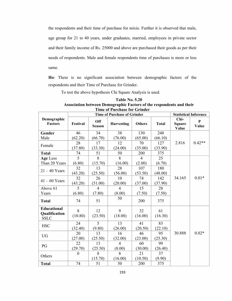
Ho: There is no significant association between demographic factors of the
respondents and their Time of Purchase for Grinder.
To test the above hypothesis Chi Square Analysis is used.
Table No. 5.20Association between Demographic Factors of the respondents and their
Time of Purchase for Grinder
DemographicFactors
Time of Purchase of Grinder Statistical Inference
Festival OffSeason Harvesting Others Total
Chi-SquareValue
PValue
GenderMale
46(62.20)
34(66.70)
38(76.00)
130(65.00)
248(66.10)
2.816 0.42**Female 28(37.80)
17(33.30)
12(24.00)
70(35.00)
127(33.90)
Total 74 51 50 200 375Age LessThan 20 Years
5(6.80)
8(15.70)
8(16.00)
4(2.00)
25(6.70)
34.165 0.01*
21 – 40 Years 32(43.20)
13(25.50)
28(56.00)
107(53.50)
180(48.00)
41 – 60 Years 32(43.20)
26(51.00)
10(20.00)
74(37.00)
142(37.90)
Above 61Years
5(6.80)
4(7.80)
4(8.00)
15(7.50)
28(7.50)
Total 74 51 50 200 375
EducationalQualificationSSLC
8(10.80)
12(23.50)
9(18.00)
32(16.00)
61(16.30)
30.888 0.02*
HSC 24(32.40)
5(9.80)
13(26.00)
41(20.50)
83(22.10)
UG 20(27.00)
13(25.50)
16(32.00)
46(23.00)
95(25.30)
PG 22(29.70)
13(25.50)
4(8.00)
60(30.00)
99(26.40)
Others 0 8(15.70)
8(16.00)
21(10.50)
37(9.90)
Total 74 51 50 200 375

194
DemographicFactors
Time of Purchase of Grinder StatisticalInference
Festival OffSeason Harvesting Others Total
Chi-SquareValue
PValue
MaritalStatusMarried
70(94.60)
47(92.20)
42(84.00)
171(85.50)
330(88.00)
5.823 0.121**Unmarried 4(5.40)
4(7.80)
8(16.00)
29(14.50)
45(12.00)
Total 74 51 50 200 375OccupationEmployee inPrivateServices
17(23.00)
8(15.70)
4(8.00)
65(32.50)
94(25.10)
70.283 0.01*
Business/Profession
20(27.00)
12(23.50)
12(24.00)
25(12.50)
69(18.40)
Employee inGovernmentServices
0 10(19.60)
4(8.00)
17(8.50)
31(8.30)
Agriculture 29(39.20)
9(17.60)
30(60.00)
51(25.50)
119(31.70)
Housewife 8(10.80)
8(15.70)
0 30(15.00)
46(12.30)
Others 0 4(7.80)
0 12(6.00)
16(4.30)
Total 74 51 50 200 375FamilyIncomeBelow Rs.5000
4(5.40)
0 0 4(2.00)
8(2.10)
59.50 0.01*
Rs. 5000 –10000
28(37.80)
8(15.70)
26(52.00)
41(20.50)
103(27.50)
Rs. 10001 –15000
12(16.20)
21(41.20)
8(16.00)
29(14.50)
70(18.70)
Rs. 15001 –20000
12(16.20)
8(15.70)
8(16.00)
45(22.50)
73(19.50)
Rs. 20001 –25000
9(12.20)
5(9.80)
8(16.00)
37(18.50)
59(15.70)
Rs. 25001 &above
9(12.20)
9(17.60) 0 44
(22.00)62
(16.50)Total 74 51 50 200 375
[Figures within bracket indicates percentage] * Significant ** Not Significant
It can be seen from the above table that there is a significant association
between age, educational qualification, occupation, family income of the respondents

195
and their time of purchase for grinder. Further it is observed that male, age group for
41 to 60 years, under graduates, employees in private sector and their family income
of Rs. 25000 and above purchase their goods as per their needs of respondents.
Gender and marital status of the respondents time of purchases is more or less same.
HYPOTHESIS 5
There is no significant association between demographic factors (Gender,
Age, Educational Qualification, Marital Status, Occupation and Family Income) of
the respondents and their Mode of Purchase of consumer durable goods (CTV,
Refrigerator, Fan, Mixie and Grinder).
5.1.5 MODE OF PURCHASE
5.1.5.1. Influence of Demographic Factors in the Mode of Purchase of
Respondents
Ho: There is no significant association between demographic factors of the
respondents and their Mode of Purchase for CTV.
To test the above hypothesis Chi Square Analysis is used.

196
Table No.5.21
Association between Demographic Factors of the respondents and their Mode of
Purchase for CTV
DemographicFactors
Mode of Purchase of CTV Statistical Inference
CashPayment
ExchangeScheme
Govt.Scheme Total
Chi-SquareValue
PValue
GenderMale
131(70.80)
100(62.10)
17(58.60)
248(66.10)
3.701 0.157**Female 54(29.20)
61(37.90)
12(41.40)
127(33.90)
Total 185 161 29 375
AgeLess Than 20Years
16(8.60)
9(5.60)
0 25(6.70)
3.701 0.157**21 – 40 Years 87
(47.00)77
47.80)16
(55.20)180
(48.00)
41 – 60 Years 69(37.30)
60(37.30)
13(44.80)
142(37.90)
Above 61Years
13(7.00)
15(9.30)
0 28(7.50)
Total 185 161 29 375EducationalQualificationSSLC
33(17.80)
28(17.40)
0 61(16.30)
71.121 0.01*
HSC 61(33.00)
17(10.60)
5(17.20)
83(22.10)
UG 51(27.60)
28(17.40)
16(55.20)
95(25.30)
PG 24(13.00)
67(41.60)
8(27.60)
99(26.40)
Others 16(8.60)
21(13.00)
0 37(9.90)
Total 185 161 29 375MaritalStatusMarried
160(86.50)
141(87.60)
29(100.00)
330(88.00)
4.383 0.112**Unmarried 25
(13.50)20
(12.40)0 45
(12.00)Total 185 161 29 375

197
DemographicFactors
Mode of Purchase of CTV Statistical InferenceCash
PaymentExchangeScheme
Govt.Scheme Total Chi-Square
ValueP
ValueOccupationEmployee inPrivateServices
25(13.50)
61(37.90)
8(27.60)
94(25.10)
61.629 0.01*
Business/Profession
45(24.30)
16(9.90)
8(27.60)
69(18.40)
Employee inGovernmentServices
9(4.90)
22(13.70)
0 31(8.30)
Agriculture 72(38.90)
34(21.10)
13(44.80)
119(31.70)
Housewife 22(11.90)
24(14.90)
0 46(12.30)
Others 12(6.50)
4(2.50)
0 16(4.30)
Total 185 161 29 375FamilyIncomeBelow Rs.5000
4(2.20)
4(2.50)
0 8(2.10)
108.32 0.01*
Rs. 5000 –10000
75(40.50)
24(14.90)
4(13.80)
103(27.50)
Rs. 10001 –15000
37(20.00%
20(12.40)
13(44.80)
70(18.70)
Rs. 15001 –20000
48(25.90%
21(13.00)
4(13.80)
73(19.50)
Rs. 20001 –25000
17(9.20%
38(23.60)
4(13.80)
73(19.50)
Rs. 25001 &above
4(2.20%
54(33.50)
4(13.80)
62(16.50)
Total 185 161 29 375[Figures within bracket indicates percentage] * Significant ** Not Significant
The above table indicates that there is a significant association between
educational qualification, occupation, family income of the respondents and their
mode of purchase for CTV. Further it is observed that business or profession, income
of Rs. 5000 to 10000 purchased their goods by cash payment. Post graduates purchase

198
their goods by exchange scheme. Gender, age group, marital status of the
respondent’s mode of purchases is more or less same.
Ho: There is no significant association between demographic factors of the
respondents and their Mode of Purchase for Refrigerator.
To test the above hypothesis Chi Square Analysis is used.
Table No.5.22
Association between Demographic Factors of the respondents and their Mode of
Purchase for Refrigerator
DemographicFactors
Mode of Purchase of Refrigerator Statistical Inference
CashPayment Loan Exchange
Scheme TotalChi-
SquareValue
PValue
GenderMale
172(72.30)
4(23.50)
56(56.00)
232(65.40)
22.023 0.01*Female 66(27.70)
13(76.50)
44(44.00)
123(34.60)
Total 238 17 100 355AgeLess Than 20Years
17 (7.10) 0 4(4.00)
21(5.90)
25.077 0.01*21 – 40 Years 95(39.90)
9(52.90)
64(64.00)
168(47.30)
41 – 60 Years 102(42.90)
8(47.10)
32(32.00)
142(40.00)
Above 61Years
24(10.10)
0 0 24(6.80)
Total 238 17 100 355EducationalQualificationSSLC
41(17.20)
4(23.50)
16(16.00)
61(17.20)
49.828 0.01*
HSC 71(29.80) 0 8
(8.00)79
(22.30)
UG 63(26.50)
4(23.50)
16(16.00)
83(23.40)
PG 46(19.30)
9(52.90)
44(44.00)
99(27.90)
Others 17(7.10) 0 16
(16.00)33
(9.30)
Total 238 17 100 355

199
DemographicFactors
Mode of Purchase of Refrigerator Statistical Inference
CashPayment Loan Exchange
Scheme TotalChi-
SquareValue
PValue
Marital StatusMarried
221(92.90)
17(100.00)
80(80.00)
318(89.60) 14.545 0.01*Unmarried 17
(7.10)0 20
(20.00)37
(10.40)Total 238 17 100 355OccupationEmployee inPrivateServices
34(14.30)
4(23.50)
52(52.00)
90(25.40)
88.185 0.01*
Business/Profession
45(18.90)
4(23.50)
12(12.00)
61(17.20)
Employee inGovernmentServices
18(7.60)
5(29.40)
8(8.00)
31(8.70)
Agriculture 103(43.30)
0 8(8.00)
111(31.30)
Housewife 26(10.90)
4(23.50)
16(16.00)
46(13.00)
Others 12(5.00)
0 4(4.00)
16(4.50)
Total 238 17 100 355FamilyIncomeBelow Rs.5000
8(3.40) 0 0 8
(2.30)
95.498 0.01*
Rs. 5000 –10000
83(34.90)
0 12(12.00)
95(26.80)
Rs. 10001 –15000
42(17.60)
4(23.50)
16(16.00)
62(17.50)
Rs. 15001 –20000
61(25.60)
4(23.50)
8(8.00)
73(20.60)
Rs. 20001 –25000
27(11.30)
0 28(28.00)
55(15.50)
Rs. 25001 &above
17(7.10)
9(52.90)
36(36.00)
62(17.50)
Total 238 17 100 355[Figures within bracket indicates percentage] * Significant ** Not Significant
It is observed from the above table that there is a significant association
between gender, age group, educational qualification, marital status, occupation,
family income of the respondents and their mode of purchase for refrigerator. Further

200
it is observed that male, age group of Rs. 41 to 60, higher secondary, married, farmers
and income of Rs. 5000 to 10000 purchased their goods by cash payment.
Ho: There is no significant association between demographic factors of the
respondents and their Mode of Purchase for Mixie.
To test the above hypothesis Chi Square Analysis is used.
Table No.5.23
Association between Demographic Factors of the respondents and their Mode of
Purchase for Mixie
DemographicFactors
Mode of Purchase of Mixie Statistical InferenceCash
PaymentExchangeScheme Total Chi-Square
ValueP
ValueGenderMale
230(65.20)
18(81.80)
248(66.10)
2.567 0.109**Female 123(34.80)
4(18.20)
127(33.90)
Total 353 22 375Age
Less Than 20Years
20(5.70)
5(22.70)
25(6.70)
11.504 0.009*21 – 40 Years 172(48.70)
8(36.40)
180(48.00)
41 – 60 Years 133(37.70)
9(40.90)
142(37.90)
Above 61 Years 28(7.90)
0 28(7.50)
Total 353 22 375EducationalQualification
SSLC
48(13.60)
13(59.10)
61(16.30)
39.199 0.01*HSC 83
(23.50) 0 83(22.10)
UG 95(26.90)
0(0.00)
95(25.30)
PG 94(26.60)
5(22.70)
99(26.40)
Others 33(9.30)
4(18.20)
37(9.90)
Total 353 22 375

201
DemographicFactors
Mode of Purchase of Mixie Statistical InferenceCash
PaymentExchangeScheme Total Chi-Square
ValueP
ValueMarital StatusMarried
308(87.30)
22(100.00)
330(88.00) 3.187 0.074**
Unmarried 45(12.70)
0 45(12.00)
Total 353 22 375OccupationEmployee inPrivate Services
89(25.20)
5(22.70)
94(25.10)
11.360 0.045*
Business/Profession
65(18.40)
4(18.20)
69(18.40)
Employee inGovernmentServices
31(8.80)
0 31(8.30)
Agriculture 106(30.00)
13(59.10)
119(31.70)
Housewife 46(13.00)
0 46(12.30)
Others 16(4.50)
0 16(4.30)
Total 353 22 375Family IncomeBelow Rs. 5000
8(2.30)
0 8(2.10)
7.050 0.217**
Rs. 5000 – 10000 94(26.60)
9(40.90)
103(27.50)
Rs. 10001 – 15000 70(19.80) 0 70
(18.70)
Rs. 15001 – 20000 69(19.50)
4(18.20)
73(19.50)
Rs. 20001 – 25000 55(15.60)
4(18.20)
59(15.70)
Rs. 25001 & above 57(16.10)
5(22.70)
62(16.50)
Total 353 22 375[Figures within bracket indicates percentage] * Significant ** Not Significant
It can be seen from the above table that there is a significant association
between age group, educational qualification, occupation of the respondents and their
mode of purchase for fan. Further it is observed that age group of Rs. 21 to 40, under
graduates, farmers purchased their goods by cash payment. Gender, marital status and
family income of the respondent’s mode of purchase are more or less same.

202
Ho: There is no significant association between demographic factors of the
respondents and their Mode of Purchase for Grinder.
To test the above hypothesis Chi Square Analysis is used.
Table No.5.24
Association between Demographic Factors of the respondents and their Mode of
Purchase for Grinder
DemographicFactors
Mode of Purchase of Grinder Statistical Inference
CashPayment
ExchangeScheme Total
Chi-SquareValue
PValue
Gender
Male
239(66.00)
9(69.20)
248(66.10)
0.058 0.810**Female 123(34.00)
4(30.80)
127(33.90)
Total 362 13 375Age
Less Than 20Years
21(5.80)
4(30.80)
25(6.70)
22.703 0.01*21 – 40 Years 180
(49.70)0 180
(48.00)
41 – 60 Years 133(36.70)
9(69.20)
142(37.90)
Above 61 Years 28(7.70)
0 28(7.50)
Total 362 13 375EducationalQualification
SSLC
57(15.70)
4(30.80)
61(16.30)
15.157 0.04*
HSC 83(22.90)
0 83(22.10)
UG 90(24.90)
5(38.50)
95(25.30)
PG 99(27.30)
0 99(26.40)
Others 33(9.10)
4(30.80)
37(9.90)
Total 362 13 375

203
DemographicFactors
Mode of Purchase of Grinder Statistical Inference
CashPayment
ExchangeScheme Total
Chi-SquareValue
PValue
Marital StatusMarried
321(88.70)
9(69.20)
330(88.00)
4.493 0.03*Unmarried 41(11.30)
4(30.80)
45(12.00)
Total 362 13 375OccupationEmployee inPrivate Services
94(26.00)
0 94(25.10)
50.907 0.01*
Business/Profession
69(19.10)
0 69(18.40)
Employee inGovernmentServices
26(7.20)
5(38.50)
31(8.300)
Agriculture 119(32.90)
0 119(31.70)
Housewife 42(11.60)
4(30.80)
46(12.30)
Others 12(3.30)
4(30.80)
16(4.30)
Total 362 13 375Family IncomeBelow Rs. 5000
8(2.20)
0 8(2.10)
17.763 0.03*
Rs. 5000 – 10000 95(26.20)
8(61.50)
103(27.50)
Rs. 10001 – 15000 70(19.30)
0 70(18.70)
Rs. 15001 – 20000 73(20.20)
0 73(19.50)
Rs. 20001 – 25000 54(14.90)
5(38.50)
59(15.70)
Rs. 25001 & above 62(17.10)
0(0.00)
62(16.50)
Total 362 13 375[Figures within bracket indicates percentage] * Significant ** Not Significant
The table indicates that there is a significant association between age group,
educational qualification, occupation and family income of the respondents and their
mode of purchase for fan. Further it is observed that age group of Rs. 21 to 40, post
graduates, farmers and income of Rs. 5000 to 10000 purchase their goods by cash

204
payment. Gender and marital status of the respondent’s mode of purchase are more or
less same.
5.6 HYPOTHESIS
There is no significant association between demographic factors (Gender,
Age, Educational Qualification, Marital Status, Occupation and Family Income) of
the respondents and their Satisfaction level of consumer durable goods (CTV,
Refrigerator, Fan, Mixie and Grinder).
5.1.6.1 INFLUENCE OF DEMOGRAPHIC FACTORS IN THE
SATISFACTION LEVEL OF RESPONDENTS
Ho: There is no significant association between demographic factors of the
respondents and their Satisfaction Level for CTV.
To test the above hypothesis Chi Square Analysis is used.
Table No. 5.25
Association between Demographic Factors of the respondents and their SatisfactionLevel for CTV
DemographicFactors
Satisfaction Level for CTV Statistical Inference
More % Less % Total %Chi-
SquareValue
PValue
GenderMale 171 59.80 60 88.2 231 66.10
22.028 0.001*Female 115 40.2 8 11.8 123 33.90Total 286 68 354AgeLess than 20 years 13 4.50 8 11.80 21 5.93
108.5 0.001*21 – 40 years 147 51.40 29 42.60 176 49.7241 – 60 Years 121 42.30 8 11.80 129 36.4461 years & More 5 1.70 23 33.80 28 7.91Total 286 68 354EducationalQualificationSSLC
53 18.50 4 5.90 57 16.10
19.807 0.011*HSC 55 19.20 19 29.70 74 20.90UG 67 23.40 24 35.30 91 25.71PG 82 28.70 13 19.10 95 26.84Others 29 10.10 8 11.80 37 10.45Total 286 68 354

205
DemographicFactors
Satisfaction Level for CTV Statistical Inference
More % Less % Total %Chi-
SquareValue
PValue
Marital StatusMarriedUnmarried
253 88.5 60 88.2 313 88.42
10.49 0.592**33 11.5 8 11.8 41 11.58
Total 286 68 354OccupationEmployee in PrivateServices
73 25.50 9 13.20 82 23.16
62.175 0.001*
Business/Profession 45 15.70 24 35.30 69 19.49Employee in Govt.Services 26 9.10 5 7.40 31 8.76
Agriculture 84 29.40 30 44.10 114 32.20Housewife 46 16.10 0 0.00 46 12.99Others 12 4.20 0 0.00 12 3.40Total 286 68 354Family IncomeBelow Rs. 5000 8 2.80 0 0.00 8 2.26
64.712 0.001*
Rs. 5000 – 10000 87 30.40 4 5.90 91 25.71Rs. 10001 -15000 37 12.90 28 41.20 65 18.36Rs. 15001 – 20000 55 19.20 14 20.60 69 19.49Rs. 20001 – 25000 41 14.30 18 26.50 59 16.67Rs. 25001 & above 58 20.30 4 5.90 62 17.51Total 286 68 354
*Significant ** Not Significant
The above table clearly shown that there is a significant association between
gender, age, educational qualification, occupation, family income and their
satisfaction level for CTV. It is observed that the male respondents, 21 to 40 years of
age group, Post Graduates, farmers, Rs. 15000 to 20000 income groups are more
satisfied with the CTV. No variation in the satisfaction level between the married and
unmarried.
Ho: There is no significant association between demographic factors of the
respondents and Satisfaction Level for Refrigerator.
To test the above hypothesis Chi Square Analysis is used.

206
Table No. 5.26
Association between Demographic Factors of the respondents and their Satisfaction
Level for Refrigerator
DemographicFactors
Satisfaction Level for Refrigerator Statistical Inference
More % Less % Total %Chi-
SquareValue
PValue
GenderMale 187 63.20 45 76.30 232 65.35
5.581 0.061**Female 109 36.80 14 23.70 123 34.65Total 296 59 355AgeLess than 20 years 13 4.40 8 13.60 21 5.92
52.365 0.001*21 – 40 years 139 47.00 29 49.20 168 47.3241 – 60 Years 132 44.60 10 16.90 142 40.0061 years & More 12 4.10 12 20.30 24 6.76Total 296 59 355EducationalQualificationSSLC
53 17.90 8 13.60 61 17.18
24.424 0.002*HSC 63 21.30 16 27.10 79 22.25UG 70 23.60 13 22.00 83 23.38PG 85 28.7 14 23.70 99 27.89Others 25 8.40 8 13.60 33 9.30Total 296 59 355Marital StatusMarriedUnmarried
263 88.90 55 93.20 318 89.5816.574 0.001*33 11.10 4 6.80 37 10.42
Total 296 59 355OccupationEmployee in PrivateServices
75 25.30 15 25.40 90 25.35
24.006 0.008*
Business/Profession 43 14.50 18 30.50 61 17.18Employee in Govt.Services 27 9.10 4 6.80 31 8.73
Agriculture 93 31.40 18 30.50 111 31.27Housewife 42 14.20 4 6.80 46 12.96Others 16 5.40 0 0.00 16 4.51Total 269 59 355Family IncomeBelow Rs. 5000 8 2.70 0 0.00 8 2.26
55.365 0.001*
Rs. 5000 – 10000 95 32.10 0 0.00 95 26.76Rs. 10001 -15000 44 14.90 18 30.50 62 17.46Rs. 15001 – 20000 50 16.90 23 39.00 73 20.56Rs. 20001 – 25000 44 14.90 11 18.60 55 15.49Rs. 25001 & above 55 18.60 7 11.90 62 17.47Total 296 59 355
*Significant ** Not Significant

207
The above table indicates that there is a significant association between age,
educational qualification, marital status, occupation, family income and their
satisfaction level for refrigerator. It is observed from the above table that 21 to 40
years of age group, post graduates, married, farmers and Rs. 5000 to 10000 are highly
satisfied about the refrigerator. No variation in the satisfaction level between the male
and female.
Ho: There is no significant association between demographic factors of the
respondents and their Satisfaction Level for Fan.
To test the above hypothesis Chi Square Analysis is used.
Table No.5.27
Association between Demographic Factors of the respondents and their Satisfaction
Level for Fan
DemographicFactors
Satisfaction Level for Fan Statistical Inference
More % Less % Total % Chi-SquareValue P Value
GenderMale 51 59.31 197 68.17 248 66.13
2.556 0.110**Female 35 40.69 92 31.83 127 33.87Total 86 289 375AgeLess than 20 years 0 0.00 25 8.65 25 6.67
16.611 0.001*21 – 40 years 51 59.30 128 44.30 179 47.7341 – 60 Years 33 38.37 109 37.72 142 37.8761 years & More 2 2.33 27 9.33 29 7.73Total 86 289 375EducationalQualificationSSLC
18 20.93 43 14.88 61 16.27
3.390 0.495**HSC 17 19.77 67 23.18 84 22.40UG 18 20.93 77 26.64 95 25.33PG 25 29.07 73 25.26 98 26.13Others 8 9.30 29 10.04 37 9.87Total 86 100.00 289 100.00 375 100.00Marital StatusMarriedUnmarried
72 83.72 257 88.93 329 87.731.106 0.293**14 16.28 32 11.07 46 12.27
Total 86 289 375

208
DemographicFactors
Satisfaction Level for Fan Statistical Inference
More % Less % Total % Chi-SquareValue P Value
OccupationEmployee inPrivate Services
22 25.58 71 24.56 93 24.80
9.835 0.080**
Business/Profession 10 11.63 59 20.41 69 18.40Employee in Govt.Services 7 8.14 24 8.30 31 8.27
Agriculture 27 31.40 93 32.18 120 32.00Housewife 12 13.95 34 11.76 46 12.27Others 8 9.30 8 2.79 16 4.26Total 86 289 375Family IncomeBelow Rs. 5000 0 0.00 8 2.80 8 2.13
4.879 0.431Rs. 5000 – 10000 25 29.07 78 27.00 103 27.47Rs. 10001 -15000 14 16.28 57 19.70 71 18.93Rs. 15001 – 20000 19 22.09 54 18.70 73 19.47Rs. 20001 – 25000 11 12.79 47 16.30 58 15.47Rs. 25001 & above 17 19.77 45 15.60 62 16.53Total 86 289 375
*Significant ** Not Significant
It can be found from the above table that there is no significant association
between gender, educational qualification, marital status, occupation, family income
and their satisfaction level for fan except the age group. It is further observed from the
above table that the age groups of 21 to 40 years are satisfied with the fan. Gender,
educational qualification, marital status, occupation and income group’s satisfaction
levels are more or less same.
Ho: There is no significant association between demographic factors of the
respondents and Satisfaction Level for Mixie.
To test the above hypothesis Chi Square Analysis is used.
209
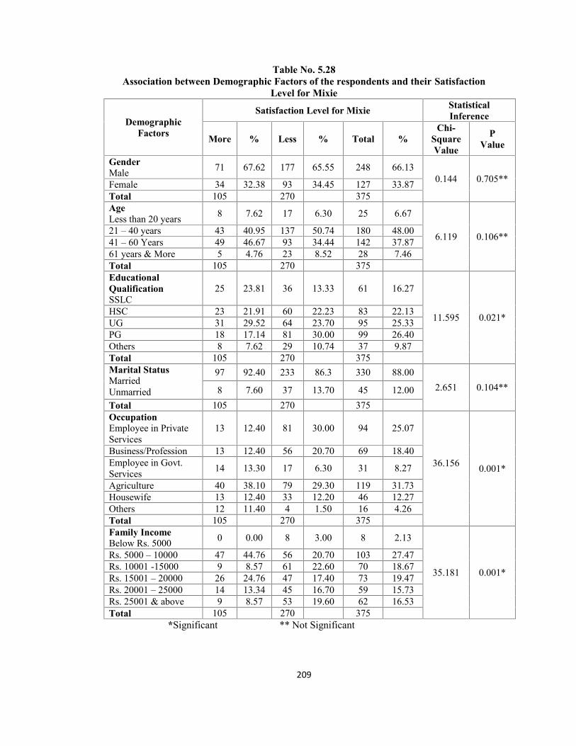
Table No. 5.28Association between Demographic Factors of the respondents and their Satisfaction
Level for Mixie
DemographicFactors
Satisfaction Level for Mixie StatisticalInference
More % Less % Total %Chi-
SquareValue
PValue
GenderMale 71 67.62 177 65.55 248 66.13
0.144 0.705**Female 34 32.38 93 34.45 127 33.87Total 105 270 375AgeLess than 20 years 8 7.62 17 6.30 25 6.67
6.119 0.106**21 – 40 years 43 40.95 137 50.74 180 48.0041 – 60 Years 49 46.67 93 34.44 142 37.8761 years & More 5 4.76 23 8.52 28 7.46Total 105 270 375EducationalQualificationSSLC
25 23.81 36 13.33 61 16.27
11.595 0.021*HSC 23 21.91 60 22.23 83 22.13UG 31 29.52 64 23.70 95 25.33PG 18 17.14 81 30.00 99 26.40Others 8 7.62 29 10.74 37 9.87Total 105 270 375Marital StatusMarriedUnmarried
97 92.40 233 86.3 330 88.002.651 0.104**8 7.60 37 13.70 45 12.00
Total 105 270 375OccupationEmployee in PrivateServices
13 12.40 81 30.00 94 25.07
36.156 0.001*
Business/Profession 13 12.40 56 20.70 69 18.40Employee in Govt.Services 14 13.30 17 6.30 31 8.27
Agriculture 40 38.10 79 29.30 119 31.73Housewife 13 12.40 33 12.20 46 12.27Others 12 11.40 4 1.50 16 4.26Total 105 270 375Family IncomeBelow Rs. 5000 0 0.00 8 3.00 8 2.13
35.181 0.001*
Rs. 5000 – 10000 47 44.76 56 20.70 103 27.47Rs. 10001 -15000 9 8.57 61 22.60 70 18.67Rs. 15001 – 20000 26 24.76 47 17.40 73 19.47Rs. 20001 – 25000 14 13.34 45 16.70 59 15.73Rs. 25001 & above 9 8.57 53 19.60 62 16.53Total 105 270 375
*Significant ** Not Significant

210
It can be found from the above table that there is no significant association
between gender, age, marital status, family income and their satisfaction level for fan
and there is a significant association between educational qualification, occupation
and family income. It can be seen from the above table that the post graduates,
farmers and income group of Rs. 5000 to 10000 are satisfied with the mixie and the
satisfaction level is more or less same among the gender, age group and marital status
of the respondents.
Ho: There is no significant association between demographic factors of the
respondents and their Satisfaction Level for Grinder.
To test the above hypothesis Chi Square Analysis is used.
Table No. 5.29Association between Demographic Factors of the respondents and their Satisfaction
Level for Grinder
DemographicFactors
Satisfaction Level for Grinder StatisticalInference
More % Less % Total %Chi-
SquareValue
PValue
GenderMale 108 63.50 140 68.30 248 66.13
0.941 0.332**Female 62 36.50 65 31.70 127 33.87Total 170 205 375AgeLess than 20 years 13 7.65 12 5.90 25 6.67
14.485 0.002*21 – 40 years 75 44.12 105 51.20 180 48.0041 – 60 Years 77 45.29 65 31.70 142 37.8661 years & More 5 2.94 23 11.20 28 7.47Total 170 205 375EducationalQualificationSSLC
33 19.41 28 13.70 61 16.27
19.193 0.001*HSC 47 27.65 36 17.60 83 22.13UG 47 27.65 48 23.40 95 25.33PG 35 20.59 64 31.20 99 26.40Others 8 4.70 29 14.10 37 9.87Total 170 205 375Marital StatusMarriedUnmarried
158 92.90 172 83.90 330 88.007.190 0.007*12 7.10 33 16.10 45 12.00
Total 170 205 375

211
DemographicFactors
Satisfaction Level for Grinder StatisticalInference
More % Less % Total %Chi-
SquareValue
PValue
OccupationEmployee in PrivateServices
30 17.60 64 31.22 94 25.06
13.930 0.016*
Business/Profession 33 19.40 36 17.56 69 18.40Employee in Govt.Services 14 8.20 17 8.29 31 8.27
Agriculture 60 35.30 59 28.78 119 31.73Housewife 21 12.40 25 12.19 46 12.27Others 12 7.10 4 1.96 16 4.27Total 170 205 375Family IncomeBelow Rs. 5000 4 2.35 4 1.95 8 2.13
43.068 0.001*
Rs. 5000 – 10000 71 41.76 32 15.61 103 27.47Rs. 10001 -15000 21 12.35 49 23.90 70 18.67Rs. 15001 – 20000 38 22.36 35 17.07 73 19.47Rs. 20001 – 25000 18 10.59 41 20.00 59 15.73Rs. 25001 & above 18 10.59 44 21.47 62 16.53Total 170 205 375
*Significant ** Not Significant
The above table indicates that there is a significant association between age,
educational qualification, marital status, occupation, family income and their
satisfaction level for grinder except gender. It is observed from the above table that 21
to 40 years of age group, post graduates, married, farmers and Rs. 5000 to 10000 are
more satisfied about the grinder. The satisfaction level is more or less same between
the male and female.
5.1.6. ROLE OF FAMILY MEMBERS OF THE RESPONDENTS IN BUYING
DECISION OF DURABLE GOODS
HYPOTHESIS 6
There is no significant difference in the ranks given by the respondent for the
role of various family members influencing the buying decision for consumer durable
goods.

212
Ho: There is no significant difference in the ranks given by the respondent for the role
of various family members influencing the buying decision for CTV.
The above hypothesis can be tested using Friedman and Kendall’s co-efficient
test.
Table No.5.30
Friedman and Kendall’s Co-efficient Concordance Test Result Regarding the
Ranking of Decision Made by the Family Members for CTV
S.No. Particulars Rank Assigned Rank
1 Self 2.71 3
2 Spouse 2.69 2
3 Children 3.70 5
4 Parents 2.32 1
5 siblings 3.57 4
Source: Compiled
N 370
Chi-square Value 216.494
df 4
Kendall’s Value W 0.146
Friedman Value P 0.01p<0.05 Significant
It is observed from the Friedman test result, the respondent ranking of various
members of their family with regard to their influence on buying decision have
significant difference at 5% level of significant.
Further the Kendall’s value (W) is very low (14.6%). Hence, it can be inferred
that the respondents are less agree for ranking given to different members in the
family with regards to buying decision for CTV.
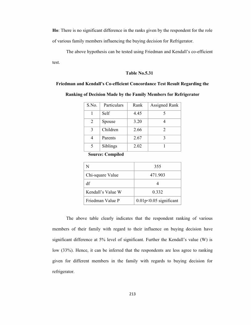
213
Ho: There is no significant difference in the ranks given by the respondent for the role
of various family members influencing the buying decision for Refrigerator.
The above hypothesis can be tested using Friedman and Kendall’s co-efficient
test.
Table No.5.31
Friedman and Kendall’s Co-efficient Concordance Test Result Regarding the
Ranking of Decision Made by the Family Members for Refrigerator
S.No. Particulars Rank Assigned Rank
1 Self 4.45 5
2 Spouse 3.20 4
3 Children 2.66 2
4 Parents 2.67 3
5 Siblings 2.02 1
Source: Compiled
N 355
Chi-square Value 471.903
df 4
Kendall’s Value W 0.332
Friedman Value P 0.01p<0.05 significant
The above table clearly indicates that the respondent ranking of various
members of their family with regard to their influence on buying decision have
significant difference at 5% level of significant. Further the Kendall’s value (W) is
low (33%). Hence, it can be inferred that the respondents are less agree to ranking
given for different members in the family with regards to buying decision for
refrigerator.
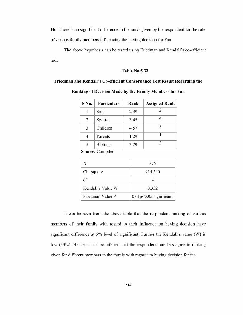
214
Ho: There is no significant difference in the ranks given by the respondent for the role
of various family members influencing the buying decision for Fan.
The above hypothesis can be tested using Friedman and Kendall’s co-efficient
test.
Table No.5.32
Friedman and Kendall’s Co-efficient Concordance Test Result Regarding the
Ranking of Decision Made by the Family Members for Fan
S.No. Particulars Rank Assigned Rank
1 Self 2.39 2
2 Spouse 3.45 4
3 Children 4.57 5
4 Parents 1.29 1
5 Siblings 3.29 3
Source: Compiled
N 375
Chi-square 914.540
df 4
Kendall’s Value W 0.332
Friedman Value P 0.01p<0.05 significant
It can be seen from the above table that the respondent ranking of various
members of their family with regard to their influence on buying decision have
significant difference at 5% level of significant. Further the Kendall’s value (W) is
low (33%). Hence, it can be inferred that the respondents are less agree to ranking
given for different members in the family with regards to buying decision for fan.

215
Ho: There is no significant difference in the ranks given by the respondent for the role
of various family members influencing the buying decision for Mixie.
The above hypothesis can be tested using Friedman and Kendall’s co-efficient
test.
Table No.5.33
Friedman and Kendall’s Co-efficient Concordance Test Result Regarding the
Ranking of Decision Made by the Family Members for Mixie
S.No. Particulars Rank Assigned Rank
1 Self 4.05 4
2 Spouse 2.00 1
3 Children 4.36 5
4 Parents 2.50 3
5 Siblings 2.08 2
Source: Compiled
N 375
Chi-square 756.033
df 4
Kendall’s Value W 0.504
Friedman Value P 0.01p<0.05 significant
The above table clearly shown that the respondent ranking of various members
of their family with regard to their influence on buying decision have significant
difference at 5% level of significant.
Further the Kendall’s value (W) is moderate (50%). Hence, it can be inferred
that the respondents are moderately agree to ranking given for different members in
the family with regards to buying decision for mixie.
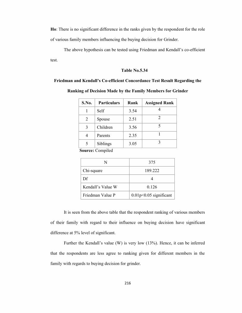
216
Ho: There is no significant difference in the ranks given by the respondent for the role
of various family members influencing the buying decision for Grinder.
The above hypothesis can be tested using Friedman and Kendall’s co-efficient
test.
Table No.5.34
Friedman and Kendall’s Co-efficient Concordance Test Result Regarding the
Ranking of Decision Made by the Family Members for Grinder
S.No. Particulars Rank Assigned Rank
1 Self 3.54 4
2 Spouse 2.51 2
3 Children 3.56 5
4 Parents 2.35 1
5 Siblings 3.05 3
Source: Compiled
N 375
Chi-square 189.222
Df 4
Kendall’s Value W 0.126
Friedman Value P 0.01p<0.05 significant
It is seen from the above table that the respondent ranking of various members
of their family with regard to their influence on buying decision have significant
difference at 5% level of significant.
Further the Kendall’s value (W) is very low (13%). Hence, it can be inferred
that the respondents are less agree to ranking given for different members in the
family with regards to buying decision for grinder.