5. kohonen’s network for modeling the auditory cortex … · 5. kohonen’s network for modeling...

5. Kohonen’s Network for Modeling the Auditory Cortex of a Bat 74

5. KOHONEN’S NETWORK FOR MODELING THEAUDITORY CORTEX OF A BAT

In this chapter we employ Kohonen’s model to simulate the projection ofthe space of the ultrasound frequencies onto the auditory cortex of a bat (Martinetz, Ritter, and Schulten 1988). The auditory cortex is the area ofthe cerebrum responsible for sound analysis ( Kandel and Schwartz, 1985).We will compare the results of the simulation with available measurementsfrom the cortex of the bat Pteronotus parnelli rubiginosus, as well as withan analytic calculation.For each animal species, the size of an area of neural units responsible forthe analysis of a particular sense strongly depends on the importance of thatsense for the species. Within each of those areas the extent of the corticalrepresentation of each input stimulus depends on the required resolution.For example, the fine analysis of the visual information of higher mammalsis accomplished in the fovea. The fovea is a very small area of the retina inthe vicinity of the optical axis with a very high density of rods and cones,the light sensitive receptors in the eye. The especially high density gives riseto a significantly higher resolution in this area than in the regions of theretina responsible for the peripheral part of the visual field. Although thefovea is only a small part of the total retina, the larger part of the visualcortex is dedicated to the processing of signals from the fovea. Similarlynonproportional representations have also been found in the somatosensorysystem and in the motor cortex. For example, particularly large areas in thesomatosensory and the motor cortex are assigned to the hand when comparedto the area devoted to the representation of other body surfaces or limbs (Woolsey 1958).In contrast no nonproportional projections have been found so far in theauditory cortex of higher mammals. The reason for this is perhaps thatthe acoustic signals perceived by most mammals contain a wide spectrumof frequencies; the signal energy is usually not concentrated in a narrowrange of frequencies. The meow of a cat, for example, is made up of many


harmonics of the base tone, and no region of the frequency spectrum playsany particular function in the cat’s survival. The auditory cortex of catswas thoroughly examined, and the result was that frequencies, as expected,are mapped onto the cortex in a linearly increasing arrangement withoutany regard for particular frequencies. The high-frequency units lie in theanterior and the low-frequency units lie in the posterior region of the cortex.According to available experimental evidence, the auditory cortex of dogsand monkeys is structured very similarly ( Merzenich et al. 1975).

5.1 The Auditory Cortex of a Bat

In bats, nonproportional projections have been detected in the auditory cor-tex. Due to the use of sonar by these animals, the acoustic frequency spec-trum contains certain intervals which are more important. Bats utilize awhole range of frequencies for orientation purposes. They can measure thedistances to objects in their surroundings by the time delay of the echo oftheir sonar signals, and they obtain information about the size of the detectedobjects by the amplitude of the echo.In addition, bats are able to determine their flight velocity relative to otherobjects by the Doppler shift of the sonar signal that they transmit. This abil-ity to determine the Doppler shift has been intensively studied in Pteronotusparnelli rubiginosus, a bat species which is native to Panama ( Suga and Jen1976). This species has developed this ability to the extent that it is able toresolve relative velocities up to 3 cm/s, enabling it to detect even the beatingof the wings of insects, its major source of nutrition. The transmitted sonarsignal consists of a pulse that lasts about 30 ms at a frequency of 61 kHz. Forthe analysis of the Doppler-shifted echoes, this bat employs a special part ofits auditory cortex ( Suga and Jen 1976).The Doppler shift ∆f of the sonar frequency by an object moving in thesame line with the bat is determined by

∆f

fe=

2vbatc− 2vobj

c. (5.1)

Here fe is the bat’s sonar frequency, i.e., 61 kHz, vbat is the bat’s velocity,vobj is the object’s flight velocity, and c is the velocity of sound. The factorof two is due to the fact that both the transmitted signal and the echo areDoppler shifted. If the bat knows its own velocity, it can determine vobj fromthe Doppler shift ∆f .


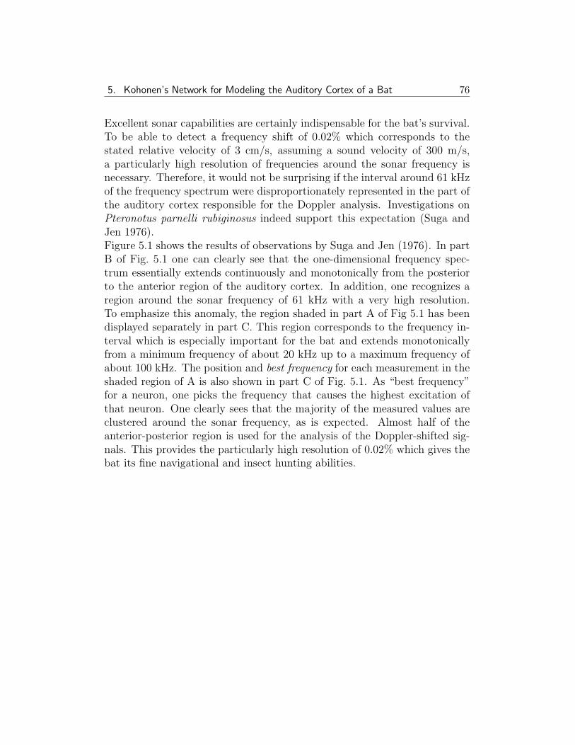
Excellent sonar capabilities are certainly indispensable for the bat’s survival.To be able to detect a frequency shift of 0.02% which corresponds to thestated relative velocity of 3 cm/s, assuming a sound velocity of 300 m/s,a particularly high resolution of frequencies around the sonar frequency isnecessary. Therefore, it would not be surprising if the interval around 61 kHzof the frequency spectrum were disproportionately represented in the part ofthe auditory cortex responsible for the Doppler analysis. Investigations onPteronotus parnelli rubiginosus indeed support this expectation (Suga andJen 1976).Figure 5.1 shows the results of observations by Suga and Jen (1976). In partB of Fig. 5.1 one can clearly see that the one-dimensional frequency spec-trum essentially extends continuously and monotonically from the posteriorto the anterior region of the auditory cortex. In addition, one recognizes aregion around the sonar frequency of 61 kHz with a very high resolution.To emphasize this anomaly, the region shaded in part A of Fig 5.1 has beendisplayed separately in part C. This region corresponds to the frequency in-terval which is especially important for the bat and extends monotonicallyfrom a minimum frequency of about 20 kHz up to a maximum frequency ofabout 100 kHz. The position and best frequency for each measurement in theshaded region of A is also shown in part C of Fig. 5.1. As “best frequency”for a neuron, one picks the frequency that causes the highest excitation ofthat neuron. One clearly sees that the majority of the measured values areclustered around the sonar frequency, as is expected. Almost half of theanterior-posterior region is used for the analysis of the Doppler-shifted sig-nals. This provides the particularly high resolution of 0.02% which gives thebat its fine navigational and insect hunting abilities.


Abb. 5.1: (A) Dorsolateral view of the bat’s cerebrum. The auditory cortexlies within the inserted rectangle. (B) Distribution of “best frequencies” on theauditory cortex, the rectangle in (A). (C) Distribution of “best frequencies” alongthe region shaded in (A) and (B). The distribution of measured values around61 kHz has been enlarged (after Suga and Jen 1976).

5.2 A Model of the Bat’s Auditory Cortex

The development of the projection of the one-dimensional frequency spaceonto the auditory cortex, with special weighting of the frequencies around61 kHz, will now be simulated by Kohonen’s model of self-organizing maps.For this purpose we will model the auditory cortex by an array of 5×25neural units.The space of input stimuli is the one-dimensional ultrasound spectrum of the


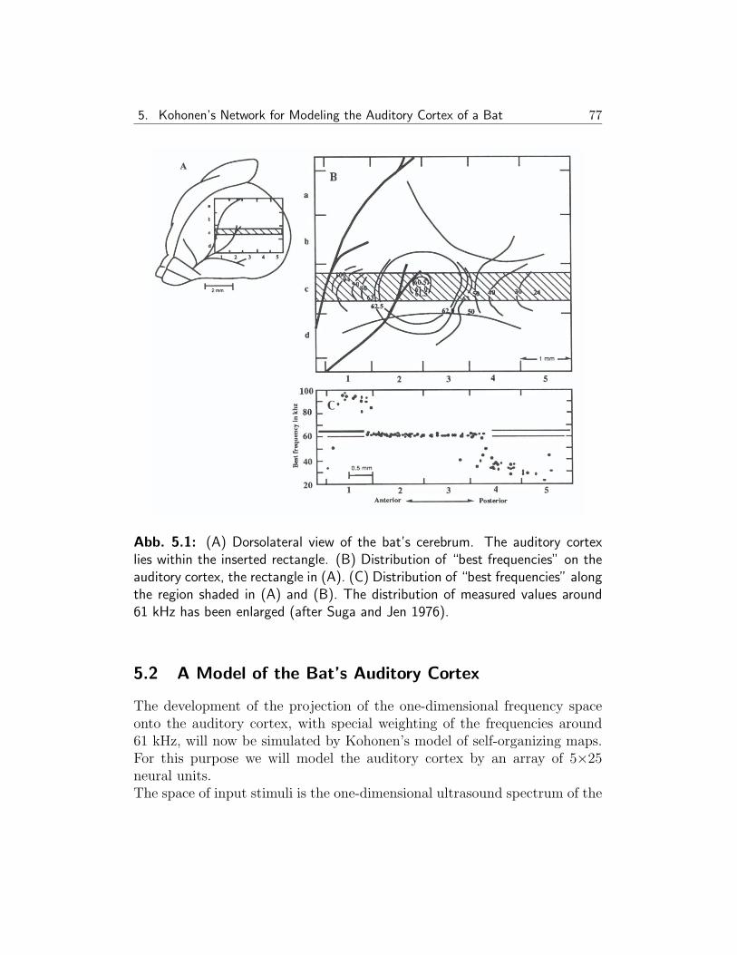
bat’s hearing. In our model this spectrum will be simulated by a Gaussiandistribution of Doppler-shifted sonar echoes on top of a white backgroundnoise. The background noise in the range from 20 to 100 kHz depicts signalsfrom external ultrasound sources. In addition, there is a peak near 61 kHzwhich consists of the echoes from objects moving relative to the bat. Wedescribe this peak of Doppler-shifted sonar signals by a Gaussian distributioncentered at 61 kHz with a width of σr=0.5 kHz. This corresponds to a rootmean square speed difference of the sonar-detected objects of about 2 m/s.Doppler-shifted sonar signals occur in our model three times as often assignals from the white background noise. Figure 5.2 shows the weightedprobability distribution.

Abb. 5.2: The relative probability density of the input signals versus frequency.Doppler-shifted echoes occur exactly three times as often as signals from thewhite background noise.

Initially, a random frequency is assigned to each model neuron of our modelcortex. This corresponds to Step 0 of Kohonen’s model as described in thelast chapter. Due to the one-dimensionality of the space of input stimuli, the


synaptic strengths wr of the model neurons r have only a single component.1

An input signal according to a probability distribution P (v) causes thatmodel neuron whose momentarily assigned frequency (the so-called “bestfrequency” of that neuron) lies closest to the input frequency to determine thecenter of the “activity peak” within which the neurons become significantlyexcited (Step 2). Next, the “best frequencies” of all neurons of the cortexare modified according to Step 3 of Kohonen’s algorithm. After a sufficientnumber of steps this modification should result in an arrangement of “bestfrequencies” on the model cortex that is continuous and is adapted to theparticular probability distribution of the input signals.

5.3 Simulation Results

In Fig. 5.1B it can be seen that the region of the auditory cortex of Pterono-tus parnelli rubiginosus responsible for the resolution of the echo is greatlyelongated, it being much more extended along the anterior-posterior axisthan it is along the perpendicular direction. A similar length-width ratio forthe model cortex was chosen in the simulation we will describe. There, theanterior-posterior length contains 25 model neurons and is five times longerthan the width of the array.Figure 5.3 shows the model cortex at different stages of the learning process.Each model neuron is represented by a box containing (the integer part of)the assigned frequency. Figure 5.3a presents the initial state. Each neuronwas assigned randomly a frequency value in the range 20 to 100 kHz. Aswe see in Fig. 5.3.b, after 500 learning steps a continuous mapping betweenthe space of input frequencies and the model cortex has already emerged.The final state, achieved after 5000 learning steps, is depicted in Fig. 5.3.c.One can see the special feature of Kohonen’s model that represents the inputstimuli on the net of neural units according to the probability with whichstimuli occur. The strong maximum of the probability density in our modelcauses a wide-ranging occupation of the “cortex” with frequencies in thenarrow interval around the sonar frequency of 61 kHz.

1 This is only an idealization that is caused by the explicit use of frequency values. Ina more realistic model one could, for example, code the frequency by different outputamplitudes of a set of overlapping filters as they are actually realized in the inner ear.The ordering process demonstrated in the simulation would, however, not be affectedby this.


Abb. 5.3: (a) (left) The initial state with random frequencies assigned to theneural units. The length-to-width ratio of the array of model neurons is five(anterior-posterior) to one (dorsolateral). Each box represents a neuron andcontains the integer part of the current “best frequency” assigned to that neu-ron. (b) (middle) The state of the “auditory cortex” after 500 learning steps.The field has evolved into a state where neighboring neurons have similar “bestfrequencies;” i.e., the space of input stimuli is represented continuously on the ar-ray. (c) (right) The “auditory cortex” in the final state, after 5000 learning steps.The region of “best frequencies” around the sonar frequency, which representsthe Doppler-shifted input signals, occupies almost half of the model cortex.

In this simulation the time dependence of the excitation zone σ and of theadaptation step widths ε were chosen as follows: σ(t) = σi[1+exp(−5 (t/tmax)

2)]and ε(t) = εi exp(−5 (t/tmax)

2) with σi = 5 and εi = 1, where t denotes thenumber of performed learning steps. The final number of learning steps atthe end of the simulation was tmax = 5000.


Abb. 5.4: The simulation results presented as in Fig. 5.1C. Along the abscissaare the positions 1 through 25 of the model neurons along the “anterior-posterior”axis. The ordinate shows the corresponding “best frequencies.” For every valuebetween 1 and 25 five frequency values are represented, one for each of the fiveneural units along the “dorso-lateral” direction.

In accordance with the experimental results from the auditory cortex ofPteronotus parnelli rubiginosus, the representation of the input frequencieson our model cortex increases monotonically along the “anterior-posterior”axis. In order to compare the results of our simulation with the mea-surements, we have presented the distribution of “best frequencies” as inFig. 5.1C. Figure 5.4 depicts the simulation results of Fig. 5.3 in the sameway as Fig. 5.1C represents the data of Fig. 5.1A-B. Each model neuronhas been described by its position 1 to 25 on the “anterior-posterior” axisas well as by its “best frequency.” This representation of the results of thesimulation produces a picture very similar to that of the experimental mea-surements (Fig. 5.1). In both cases a plateau arises that occupies almosthalf of the cortex and contains the neural units specialized in the analysisof the Doppler-shifted echoes. The size of this plateau is determined by theshape of the probability distribution of the input stimuli. In Section 5.4 wewill look more closely at the relation between the shape of the probabilitydistribution and the final cortical representation in Kohonen’s model.


5.4 Mathematical Description of the “CorticalRepresentation”

We want to investigate what mappings between a neural lattice and an in-put signal space result asymptotically for Kohonen’s model. For “maxi-mally ordered” states we will demonstrate a quantitative relation betweenthe “neural-occupation density” in the space of input stimuli which corre-sponds to the local enlargement factor of the map, and the functional formof the probability density P (v) of the input signals ( Ritter and Schulten1986a). The result will enable us to derive an analytical expression for theshape of the curve shown in Fig. 5.4, including the size of the plateau. Un-fortunately, such analytical expressions will be limited to the special case ofone-dimensional networks and one-dimensional input spaces. The followingderivation is mainly directed at the mathematically inclined reader; it canbe skipped without loss of continuity.To begin, we consider a lattice A of N formal neurons r1, r2,. . . , rN . A map φw : V 7→ A of the space V onto A, which assigns to eachelement v ∈ V an element φw(v) ∈ A, is defined by the synaptic strengthsw = (wr1 ,wr2 , . . . ,wrN ), wrj ∈ V . The image φw(v) ∈ A that belongs tov ∈ V is specified by the condition

‖wφw(v) − v‖ = minr∈A‖wr − v‖, (5.2)

i.e., an element v ∈ V is mapped onto that neuron r ∈ A for which ‖wr−v‖becomes minimal.As described in Chapter 4, φw emerges in a learning process that consistsof iterated changes of the synaptic strengths w = (wr1 ,wr2 , . . . ,wrN ). Alearning step that causes a change from w′ to w can formally be describedby the transformation

w = T(w′,v, ε). (5.3)

Here v ∈ V represents the input vector invoked at a particular instance, andε is a measure of the plasticity of the synaptic strengths (see Eq. (4.15).The learning process is driven by a sequence of randomly and independentlychosen vectors v whose distribution obeys a probability density P (v). Thetransformation (5.3) then defines a Markov process in the space of synapticstrengths w ∈ V ⊗V ⊗ . . .⊗V that describes the evolution of the map φw(v).We will now show that the stationary state of the map which evolves asymp-


totically by this process can be described by a partial differential equationfor the stationary distribution of the synaptic strengths.Since the elements v occur with the probability P (v), the probabilityQ(w,w′)for the transition of a state w′ to a state w, via adaptation step (5.3), is givenby

Q(w,w′) =∫δ(w −T(w′,v, ε))P (v) dv. (5.4)

δ(x) denotes the so-called delta-function which is zero for all x 6= 0 and forwhich

∫δ(x)dx = 1. More explicitly, Eq. (5.3) can be written

wr = w′r + ε hrs(v −w′r) for all r ∈ A. (5.5)

Here s = φw′(v) is the formal neuron to which v is assigned in the old mapφw′ .In the following we take exclusive interest in those states φw that correspondto “maximally ordered maps,” and we want to investigate their dependenceon the probability density P (v). We assume that the space V and the lat-tice A have the same dimensionality d. A “maximally ordered map” canthen be characterized by the condition that lines in V which connect the wr

of r adjacent in the network are not allowed to cross. Figure 5.5 demon-strates this fact with an example of a two-dimensional Kohonen lattice ona two-dimensional space V of input stimuli with a homogeneous probabilitydistribution P (v). The square frame represents the space V . The synapticstrengths wr ∈ V determine the locations on the square which are assignedto the formal neurons r ∈ A. Each mesh point of the lattice A correspondsto a formal neuron and, in our representation, is drawn at the location thathas been assigned to that neuron through wr. Two locations wr are con-nected by a line if the two corresponding formal neurons r are neighbors inthe lattice A. Figure 5.5a shows a map that has reached a state of “maximalorder” as seen by the lack of line crossings between lattice points. In contrastFig. 5.5b presents a map for which even in the final stage some connectionsstill cross. Such a map is not “maximally ordered.”In the following calculation we will make a transition from discrete values of rto continuous ones. This is possible because in the following we restrict our-selves to “maximally ordered” states where in the transition to a continuumwr becomes a smooth function of the spatial coordinate r in the network.


Abb. 5.5: An example for a “maxi-mally ordered” state of the network.Network and input signals are bothtwo-dimensional. All input signalsoriginate from the limiting square.In the continuum limit the networknodes are infinitely dense and spec-ify a one-to-one mapping between thenetwork and the square.

Abb. 5.6: An example of an incom-pletely ordered state of the network,evolved as a consequence of the rangeσ(t) of hrs to be too short initially(see Eq. (68)). In this case a topo-logical defect develops and the con-nections between neighboring latticepoints cross. In the continuum limita one-to-one mapping cannot be ob-tained.

We consider an ensemble of maps that, after t learning steps, are all in thevicinity of the same asymptotic state and whose distribution is given by adistribution function S(w, t). In the limit t→∞, S(w, t) converges towardsa stationary distribution S(w) with a mean value w̄. In Chapter 14 we willshow that the variance of S(w) under the given conditions will be of theorder of ε. Therefore, for an ε that is sufficiently slowly approaching zero,all members of the ensemble will result in the same map characterized by itsvalue w̄.We want to calculate w̄ in the limit ε → 0. In the stationary state, thecondition S(w) =

∫Q(w,w′)S(w′) dw′ holds, and, therefore, it also holds

thatw̄ =

∫wS(w) dw =

∫ ∫wQ(w,w′)S(w′) dwdw′. (5.6)


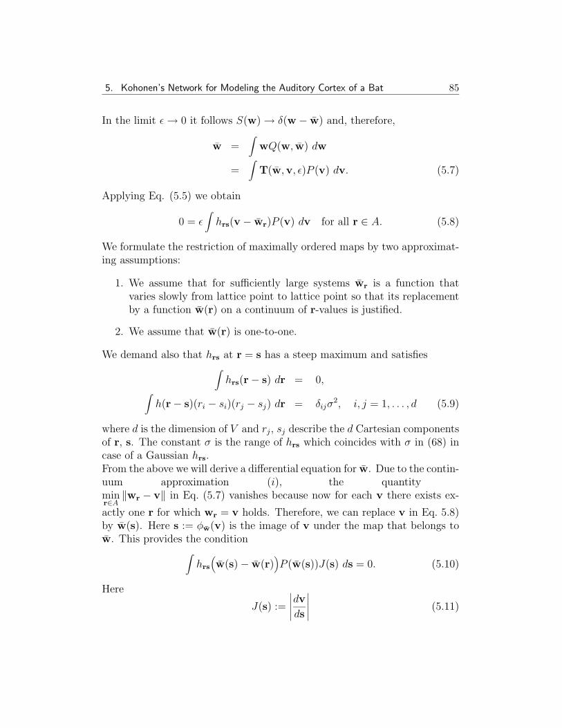
In the limit ε→ 0 it follows S(w)→ δ(w − w̄) and, therefore,

w̄ =∫

wQ(w, w̄) dw

=∫

T(w̄,v, ε)P (v) dv. (5.7)

Applying Eq. (5.5) we obtain

0 = ε∫hrs(v − w̄r)P (v) dv for all r ∈ A. (5.8)

We formulate the restriction of maximally ordered maps by two approximat-ing assumptions:

1. We assume that for sufficiently large systems w̄r is a function thatvaries slowly from lattice point to lattice point so that its replacementby a function w̄(r) on a continuum of r-values is justified.

2. We assume that w̄(r) is one-to-one.

We demand also that hrs at r = s has a steep maximum and satisfies∫hrs(r− s) dr = 0,∫

h(r− s)(ri − si)(rj − sj) dr = δijσ2, i, j = 1, . . . , d (5.9)

where d is the dimension of V and rj, sj describe the d Cartesian componentsof r, s. The constant σ is the range of hrs which coincides with σ in (68) incase of a Gaussian hrs.From the above we will derive a differential equation for w̄. Due to the contin-uum approximation (i), the quantityminr∈A‖wr − v‖ in Eq. (5.7) vanishes because now for each v there exists ex-

actly one r for which wr = v holds. Therefore, we can replace v in Eq. 5.8)by w̄(s). Here s := φw̄(v) is the image of v under the map that belongs tow̄. This provides the condition∫

hrs

(w̄(s)− w̄(r)

)P (w̄(s))J(s) ds = 0. (5.10)

Here

J(s) :=

∣∣∣∣∣dvds∣∣∣∣∣ (5.11)


is the absolute value of the Jacobian of the map φw̄. With q := s − r as anew integration variable and P̄ (r) := P (w̄(r)) the expansion of Eq. (5.10)in powers of q yields (with implicit summation over repeated indices; e.g.,qi∂i is to be summed over all values of i)

0 =∫hq0(qi∂iw̄ +

1

2qiqj∂i∂jw̄ + . . .) ·

·(P̄ + qk∂kP̄ + . . .) · (J + ql∂lJ + . . .) dq

=∫hq0qiqj dq ·

((∂iw̄)∂j(P̄ J) +

1

2P̄ J · ∂i∂jw̄

)(r) +O(σ4)

= σ2 ·[(∂iw̄)(∂i(P̄ J) +

1

2P̄ J · ∂2

i w̄)](r) +O(σ4), (5.12)

where we made use of (81). In order for the expansion (5.12) to hold it isnecessary and sufficient for small σ that condition

∑i

∂iw̄

(∂iP̄

P̄+∂iJ

J

)= −1

2

∑i

∂2i w̄ (5.13)

or, with the Jacobi matrix Jij = ∂jw̄i(r) and ∆ =∑i∂2i , condition

J · ∇ ln(P̄ · J) = −1

2∆w̄ (5.14)

is satisfied. For the one-dimensional case we obtain J = J = dw̄/dr and∆w̄ = d2w̄/dr2 with w̄ and r as scalars. In this case the differential equation(5.14) can be solved. For this purpose we rewrite (5.14) and obtain

dw̄

dr

1

P

dP̄

dr+

(dw̄

dr

)−1d2w̄

dr2

= −1

2

d2w̄

dr2(5.15)

from which we can conclude

d

drln P̄ = −3

2

d

drln

(dw̄

dr

). (5.16)

This result allows us to determine the local enlargement factor of the mapin terms of the generating probability distribution P (v).Since φw̄(w̄(r)) = r holds, the local enlargement factor M of φw̄ can bedefined byM = 1/J (compare Eq. (5.11)). For the one-dimensional caseM =


(dw̄/dr)−1 and we obtain as a relation between input stimulus distributionand cortical representation

M(v) = J−1 =dr

dw̄∝ P (v)2/3. (5.17)

The local enlargement factor M(v) depends on the probability density P (v)according to a power law. It can be shown that the exponent 2/3 that wefound in the continuum approximation undergoes a correction for a discreteone-dimensional system and is then given by 2

3− [3(1 + n2)(1 + [n+ 1]2)]−1,

where n is the number of neighbors that are taken into account on each sideof the excitation center, (i.e., hrs = 1 for ‖r − s‖ ≤ n and zero elsewhere)(Ritter 1989). The continuum corresponds to the limit of infinite density ofneighbors. Then n = ∞ for each finite σ and we obtain the previous resultof 2/3.

5.5 “Cortical Representation” in the Model of the Bat’sAuditory Cortex

We now apply the mathematical derivation of Section 5.4 to the particu-lar input stimulus distribution that we assumed for our model of the bat’sauditory cortex and compare the result with a simulation.The input stimulus distribution that we assume can be written in the rangev1 ≤ v ≤ v2 as

P (v) =P0

v2 − v1

+ (1− P0)1√

2πσrexp

(−(v − ve)2

2σ2r

)(5.18)

with the parameters σr=0.5 kHz, ve=61.0 kHz, v1=20 kHz,v2=100 kHz and P0=1/4. The width of the distribution of the Doppler-shifted echoes is given by σr, and P0 is the probability for the occurrence ofan input stimulus from the white background noise. v1 and v2 are the limitsof the ultrasound spectrum that we assume the bat can hear.The integral I =

∫ v2v1P (v)dv is not exactly unity because of the finite inte-

gration limits. Since, due to the small σr of 0.5 kHz, nearly all the Doppler-shifted echo signals lie within the interval [20, 100] and the deviation of Ifrom unity is negligible. With the choice P0 = 1/4, the Doppler-shifted sig-nals occur three times as often as signals due to the background noise (see


also Fig. 5.2). From Eqs. (5.17) and (5.18) we find

dr

dw̄= C ·

(P0

v2 − v1

+ (1− P0)1√

2πσrexp

(−(v − ve)2

2σ2r

))2/3

(5.19)

where C is a proportionality constant. In integral form one has

r(w̄)− r1 = C ·w̄∫

w̄1

(P0

v2 − v1

+1− P0√

2πσr

× exp

(−(v − ve)2

2σ2r

))2/3

dv. (5.20)

We will solve this integral numerically and then compare the resulting w̄(r)with the corresponding values from a simulation.Since these considerations apply only to the case where the dimensionalityof the net and the dimensionality of the space of input stimuli is identical,we stretch the “auditory cortex” and, instead of a 5×25 net as in Figs. 5.3and 5.4, assume a one-dimensional chain with 50 elements for the presentsimulation. Starting from a linear, second-order differential equation, we needtwo boundary conditions, e.g., w̄1(r1) and w̄2(r2), from our simulation datato be able to adjust the function r(w̄) of Eq. (5.20) uniquely. Since boundaryeffects at the beginning and the end of the chain were not taken into accountin our analytic calculation, the end points can in some cases deviate slightlyfrom our calculated curve. To adjust the curve to the simulation data, wetake values for w1 and w2 that do not lie too close to the end points; in thiscase we have chosen w̄ at the third and forty-eighth link of the chain, i.e.,at r1 = 3 and r2 = 48. The solid curve in Fig. 5.6 depicts the function w̄(r)calculated numerically from Eq.(5.20) and adjusted to the simulation data.The dots show the values w̄r that were obtained by simulating the Markovprocess (75). The representation corresponds to the one in Fig. 5.4. The timedependence of the excitation zone σ and of the adaptation step width ε forthe simulation were chosen as follows: σ(t) = σi[1 + exp(−(5t/tmax)

2)] withσi = 10, ε(t) = εi exp(−(5t/tmax)

2) with εi = 1. For the maximal number oflearning steps tmax = 20000 was chosen.


Abb. 5.7: A bat’s sensitivity to accoustic and sonar signals (cf. Fig. 5.4). Thesolid curve represents the function w̄(r) calculated from Eq. (92). The dots showthe values obtained from simulating the Markov process (75). For comparisonwe show the result for M(v) ∝ P (v) with a dashed line. This result stronglydeviates from the simulation data.

Clearly, the function w̄(r) resulting from Eq. (5.20) is in close agreementwith the simulation results, and even the deviations at the end points aresmall. One may have expected intuitively that for the magnification holdsM(v) ∝ P (v), i.e., a magnification proportional to the stimulus density. Thecorresponding result is presented in Fig. 5.6 as well to demonstrate that thisexpectation is, in fact, incorrect.For the present input stimulus distribution, it is possible to estimate the sizeof the region relevant for the analysis of the Doppler-shifted signal, i.e., theextension of the 61 kHz plateau in Fig. 5.6. In Eq. 5.20) we integrate overP (v)2/3 and, therefore, the function r(w̄) increases sharply for large valuesof P (v). Hence, the plateau starts where the Gaussian distribution of theDoppler-shifted echoes increases strongly relative to the background. This isapproximately the case for v = ve−2σr. Accordingly, the plateau ends wherethe Gaussian peak recedes back into the homogeneous background, i.e., atv = ve + 2σr. Therefore, the relation

∆rplateau = C ·ve+2σr∫ve−2σr

(P0

v2 − v1

+ (1− P0)1√

2πσr


× exp

(−(v − ve)2

2σ2r

))2/3

dv (5.21)

for the size of the plateau holds. Within these integration limits the back-ground portion in the integrand is negligible compared to the values of theGaussian. Furthermore, we can extend the integration of the integrand thatresults without the background towards infinity without significant error.The integral can then be evaluated, yielding the approximation

∆rplateau ≈ C · (1− P0)2/3

∞∫−∞

1

(√

2πσr)2/3exp

(−2

3

v2

2σ2r

)dv

≈ C ·√

3

2

(√2πσr(1− P0)2

)1/3. (5.22)

In order to determine the part of the plateau relative to the overall “auditorycortex,” we also need an estimate of the integral in Eq. (5.20), where we haveto integrate over the full band width of input frequencies. To obtain this wesplit the integration range from v1=20 kHz to v2=100 kHz into three regionsas follows

∆rtotal ∝ve−2σr∫v1

(P (v))2/3 dv +

ve+2σr∫ve−2σr

(P (v))2/3 dv

+

v2∫ve−2σr

(P (v))2/3 dv. (5.23)

We have already estimated the second integral in the sum by Eq. (5.22).Within the integration limits of the other two integrals the contribution ofthe Gaussian distribution is so small that it can be neglected relative to thebackground. In addition, σr � (v2 − v1), enabling us to write

∆rtotal ≈ ∆rplateau + C · (v2 − v1)(

P0

v2 − v1

)2/3

≈ ∆rplateau + C · P02/3(v2 − v1)1/3. (5.24)

If we insert the parameters of our above model of the input stimulus distri-bution of the bat into the two estimates (5.22) and (5.24), we obtain for thesize of the 61 kHz region, relative to the size of the total “cortex,” the value

∆rplateau∆rtotal

≈ 39%.


This implies that for our case of a 50-unit chain, the plateau should consistof 19 to 20 neurons. This value agrees very well with the simulation resultspresented in Fig. 5.6.By now we have extensively described the basics of Kohonen’s model—theself-organization of a topology-conserving map between an input stimulusspace and a network of neural units. We have compared the simulation re-sults of Kohonen’s model to experimental data as well as to a mathematicaldescription valid for certain limiting cases. The simulation data have agreedat least qualitatively with the experimental findings. More than a qualitativeagreement should not have been expected, considering the many simplifica-tions of Kohonen’s model. In contrast to that, the mathematical result for therepresentation of the input signals relative to their probability corresponds,even quantitatively, very well to the results obtained from simulations.In Chapter 6 we will become acquainted with a completely different appli-cation of Kohonen’s model. Instead of a mappingonto a continuum, we willgenerate a mapping that projects a linear chain onto a discrete set of points.Such a mapping can be interpreted as a choice of a connection path betweenthe points. The feature of the algorithm to preserve topology as much aspossible manifests itself in a tendency to minimize the path-length. In thisway, very good approximate solutions for the well-known travelling salesmanproblem can be achieved.

5. kohonen’s network for modeling the auditory cortex … · 5. kohonen’s network for modeling...

Documents