5. Intermediate Value Property for Derivatives

When we sketched graphs of speciÞc functions, we determined the sign of aderivative or a second derivative on an interval (complementary to the criticalpoints) using the following procedure: We checked the sign at one point in theinterval and then appealed to the Intermediate Value Theorem (Theorem 5.2)to conclude that the sign was the same throughout the interval. This works Þneas long as the derivatives are continuous. Can a derivative fail to be continuous?If so, is there a systematic way to check signs for such a derivative in order toapply various tests easily? (I am referring to the tests in Theorem 10.19 andCorollary 10.31.)The answer to the Þrst question is yes, a derivative can fail to be continuous.

The answer to the second question is that the answer to the Þrst question isirrelevant: We can determine the sign of a derivative on an interval the way aswe always did � by checking the sign at only one point of the interval � whetherthe derivative is continuous or not! In other words, derivatives do not changesign on an interval on which they are deÞned without having value zero at somepoint of the interval.We give an example that veriÞes our answer to the Þrst question, and we

give a theorem that explains our answer to the second question.

Example 10.48: We give an example of a differentiable function f : R1 →R1 such that its derivative is not continuous. DeÞne f by

f(x) =

½x2 sin( 1

x) , if x 6= 00 , if x = 0.

Using various results in Chapter VII and Theorem 8.20, we see that f isdifferentiable at every point x 6= 0 and that

f 0(x) = x2[cos( 1x)](

−1x2 ) + 2x sin(

1x) = 2x sin(

1x)− cos( 1

x), x 6= 0.furthermore, we see that f is differentiable at x = 0 as follows: For x 6= 0,

0 ≤¯̄̄f(x)−f(0)

x−0

¯̄̄=¯̄x sin( 1

x)¯̄ ≤ |x|;

thus, since limx→0 |x| = 0, the Squeeze Theorem (Theorem 4.34) applies to giveus that

limx→0

¯̄̄f(x)−f(0)

x−0

¯̄̄= 0.

This proves that f 0(0) = 0 (recall Exercise 6.10).Finally, we show that f 0 is not continuous at 0 by showing that limx→0 f

0(x)does not exist. Recall that

f 0(x) = x2[cos( 1x)](

−1x2 ) + 2x sin(

1x) = 2x sin(

1x)− cos( 1

x), x 6= 0.Note that

101

0 ≤ ¯̄2x sin( 1x)¯̄ ≤ |2x|, x 6= 0;

thus, since limx→0 |2x| = 0, we have by the Squeeze Theorem (Theorem 4.34)that

limx→0 2x sin(1x) = 0.

Hence, if limx→0 f0(x) existed, then we would have

limx→0 cos(1x)

4.2= limx→0 2x sin(

1x)− limx→0 f

0(x),

which is impossible (since, as is clear, limx→0 cos(1x) does not exist).

Next, we show why, even though derivatives may not be continuous, we candetermine the sign of a derivative on an interval complementary to the criticalpoints by checking the sign at only one point of the interval. The reason issimple enough � derivatives, continuous or not, satisfy the conclusion to theIntermediate Value Theorem (Theorem 5.2). We prove this in Theorem 10.50.First, we introduce relevant terminology and discuss the notion we deÞne. (Theterminology carries the name of the French mathematician G. Darboux (1842 -1917) who proved the theorem we will prove.)

DeÞnition: Let I be an interval, and let f : I → R1 be a function. We saythat f is a Darboux function provided that for any two points p, q ∈ I and anypoint y between f(p) and f(q), there is a point x between p and q such thatf(x) = y (i.e., for any subinterval J of I, f(J) is an interval).

There are fairly simple functions that are Darboux but not continuous: Forexample, let

f(x) =

½sin( 1

x) , if x 6= 00 , if x = 0.

Actually, the derivative f 0 of the function in Example 10.48 is another ex-ample of a discontinuous Darboux function. This fact about the function inExample 10.48 illustrates the content of the theorem we will prove: Any deriva-tive on an interval is a Darboux function.We use the following lemma in the proof of our theorem.

Lemma 10.49: Let f be a continuous function on an interval I , and let Cdenote the set of all slopes of chords joining any two points on the graph of f ;that is,

C = { f(s)−f(r)s−r : s, r ∈ I and s 6= r}.

Then C is an interval.

Proof: Fix p ∈ C, say

p = f(a)−f(b)a−b , a < b.

102

We show that there is an interval in C joining p to any other point of C. Tothis end, let z ∈ C, say

z = f(u)−f(v)u−v , u < v.

Note that since a− b < 0 and u− v < 0, [1− t](a− b) + t(u− v) 6= 0 for allt ∈ [0, 1]; in anticipation of what comes next, we write this as follows:

[1− t]a+ tu− [1− t]b− tv 6= 0 for all t ∈ [0, 1].

Hence, the following formula deÞnes a function σ : [0, 1]→ C such that σ(0) = pand σ(1) = z as follows:

σ(t) = f([1−t]a+tu)−f([1−t]b+tv)[1−t]a+tu−[1−t]b−tv , all t ∈ [0, 1].

By the continuity of f and by various theorems about continuity in ChapterIV (notably, 4.4, 4.21 and 4.28), we see that σ is continuous. Thus, by theIntermediate Value Theorem (Theorem 5.2), σ([0, 1]) is an interval. Therefore,since σ(0) = p and σ(1) = z, we have proved that p and any other point z of Clie in an interval in C. It now follows easily that C is an interval. ¥Theorem 10.50: If f is a differentiable function on an interval I, then f 0

is a Darboux function.

Proof: Let D be the set of all values of the Þrst derivative of f on I,

D = {f 0(x) : x ∈ I}.

We prove that D is an interval, which is simply another way of stating thetheorem we are proving.Let C be as in Lemma 10.49. Since f is continuous by Theorem 6.14, C is

an interval by Lemma 10.49. Let E denote the set of end points of C (E maybe empty).The Mean Value Theorem (Theorem 10.2) says that C ⊂ D. The deÞnition

of the derivative says that every value of the Þrst derivative of f is a limit ofslopes of chords; hence, D ⊂ C ∪E (since C ∪E = C∼, where C∼ is the set ofall points arbitrarily close to C, as deÞned in sections 1 and 2 of Chapter II).We have proved that

C is an interval and C ⊂ D ⊂ C ∪E.

Therefore, it follows at once that D is an interval. ¥In Exercise 10.16 you were asked if a certain function with a simple discon-

tinuity was a derivative of some function. You probably worked the exercise ina fairly computational way. Theorem 10.50 yields the solution to Exercise 10.16immediately and furnishes a completely different perspective on the exercise.We brießy discuss the situation in general.

103

Let f be a function deÞned on an open interval I. Then f is said to havea simple discontinuity at a point p ∈ I, sometimes called a discontinuity ofthe Þrst kind, provided that f is not continuous at p and limx→p− f(x) andlimx→p+ f(x) exist. The function f is said to have a discontinuity of the secondkind at p provided that f is not continuous at p and f does not have a simplediscontinuity at p.There are exactly two ways a function can have a simple discontinuity at p :

Either limx→p− f(x) 6= limx→p+ f(x) or limx→p− f(x) = limx→p+ f(x) 6= f(p).Corollary 10.51: If f is a differentiable function on an open interval I,

then f 0 has no simple discontinuities.Proof: Left as the Þrst exercise below. ¥Exercise 10.52: Prove Corollary 10.51. In fact, prove that the corollary ex-

tends to all Darboux functions; that is, any discontinuity of a Darboux functionon an open interval is a discontinuity of the second kind.

Exercise 10.53: A differentiable function on R1 can have derivative equal tozero at a point and yet not have a local extremum at the point (e.g., f(x) = x3).Similarly, a differentiable function on R1 can have a positive derivative at a pointwithout being strictly increasing in any neighborhood of the point (compare withTheorem 10.17): Modify the function in Example 10.48 to give an example.(Hint: Think geometrically: modify the graph of the function in Example

10.48.)

Exercise 10.54: DeÞne f : [ 910 ,

2110 ]→ R1 by f(x) = x4 − 6x3 + 12x2. Find

D = {f 0(x) : x ∈ [ 910 ,

2110 ]}, C = { f(s)−f(r)

s−r : s, r ∈ [ 910 ,

2110 ] and s 6= r};

D and C are the sets in the proof of Theorem 10.50.

Exercise 10.55: Let f : R1 → R1 be a polynomial of odd degree. Theorem10.50 implies that the set D of all values of the Þrst derivative of f is an interval.What types of intervals can D be? What types of intervals can the set C inLemma 10.49 be?

Exercise 10.56: Repeat Exercise 10.55 for the case when f is a polynomialof even degree.

Exercise 10.57: Prove that at most one of the functions f and g below canbe a derivative of a function:

f(x) =

sin(1

x) , if x 6= 0

0 , if x = 0g(x) =

sin(1

x) , if x 6= 0

1 , if x = 0.

104

Chapter XI: Area

The chapter is a bridge between previous chapters and the topic of sub-sequent chapters (the integral). We simply present an informal, nonrigorousdiscussion of an aspect of area for the purpose of motivating the integral. Ourdiscussion connects derivatives with area!Consider the continuous function f whose graph we have drawn in Figure 1

below. We want to Þnd the area between the graph of f and the interval [a, b]on x - axis.

Figure 1

There is an obvious question here: What do we mean by area (referringto the area between the graph of f and the interval [a, b])? We will answerthe question in a precise way in Chapter XIV. Here we answer the questionsomewhat intuitively, and then we describe how to compute the area.We start by dividing the interval [a, b] into n intervals whose end points are

x0 = a < x1 < x2 < · · · < xn = b.

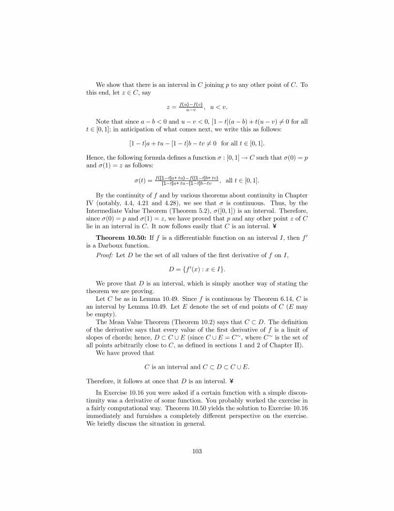
We think of each of the intervals [xi−1, xi] as being small, and we consider therectangles Ri of height f(xi) and width xi − xi−1, as in Figure 2 (we use f(xi)as a matter of convenience; we could use f(ti) for any ti ∈ [xi−1, xi]).

105

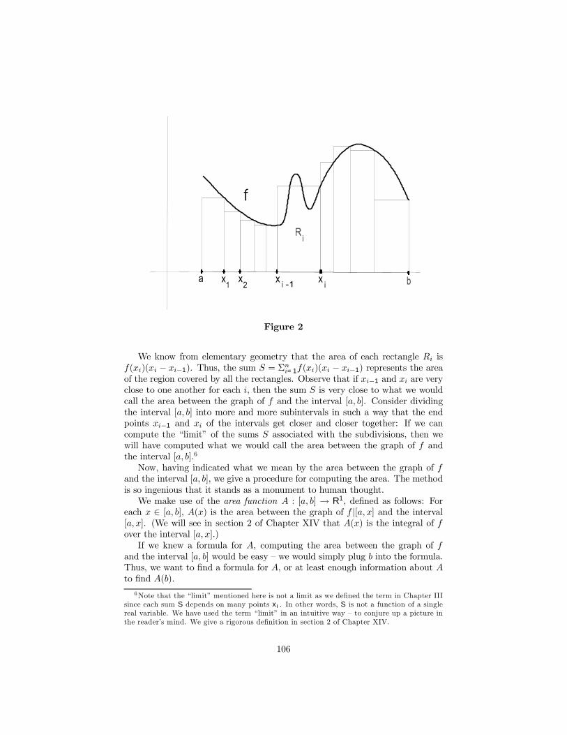
Figure 2

We know from elementary geometry that the area of each rectangle Ri isf(xi)(xi − xi−1). Thus, the sum S = Σni=1f(xi)(xi − xi−1) represents the areaof the region covered by all the rectangles. Observe that if xi−1 and xi are veryclose to one another for each i, then the sum S is very close to what we wouldcall the area between the graph of f and the interval [a, b]. Consider dividingthe interval [a, b] into more and more subintervals in such a way that the endpoints xi−1 and xi of the intervals get closer and closer together: If we cancompute the �limit� of the sums S associated with the subdivisions, then wewill have computed what we would call the area between the graph of f andthe interval [a, b].6

Now, having indicated what we mean by the area between the graph of fand the interval [a, b], we give a procedure for computing the area. The methodis so ingenious that it stands as a monument to human thought.We make use of the area function A : [a, b] → R1, deÞned as follows: For

each x ∈ [a, b], A(x) is the area between the graph of f |[a, x] and the interval[a, x]. (We will see in section 2 of Chapter XIV that A(x) is the integral of fover the interval [a, x].)If we knew a formula for A, computing the area between the graph of f

and the interval [a, b] would be easy � we would simply plug b into the formula.Thus, we want to Þnd a formula for A, or at least enough information about Ato Þnd A(b).

6Note that the �limit� mentioned here is not a limit as we deÞned the term in Chapter IIIsince each sum S depends on many points xi. In other words, S is not a function of a singlereal variable. We have used the term �limit� in an intuitive way � to conjure up a picture inthe reader�s mind. We give a rigorous deÞnition in section 2 of Chapter XIV.

106

We �show� that the area function A is differentiable by �computing� itsderivative (the quotes mean we show and compute as best as we can without amathematically precise deÞnition of area). Then we discover what the derivativeof A has to do with Þnding the area we want.Fix x ∈ [a, b]. In order to Þnd

A0(x) = limh→0A(x+h)−A(x)

h ,

it is clear that we must write the numerator with a factor of h.We Þrst examine the numerator A(x+ h)−A(x) for some given h > 0; we

assume h to be near enough to 0 so that x+ h < b (if x = b, we only considerthe case when h < 0, which we will consider later for any x).We see from Figure 3 that A(x+h)−A(x) is the area between the graph of

f |[x, x+ h] and the interval [x, x+ h].

Figure 3

The continuous function f has a maximum value M and a minimum valuem on [x, x+h] (by Theorem 5.13). Consider the function ϕ : [m,M ]→ R1 thatassigns to a point t ∈ [m,M ] the area of the rectangle [x, x + h] × [0, t] (seeFigure 4); since the height of the rectangle is t and its width is h,

ϕ(t) = th for each t ∈ [m,M ].

107

Figure 4

We know that the function ϕ is continuous (see Example 2.23); furthermore,since A(x + h) − A(x) is the area between the graph of f |[x, x + h] and theinterval [x, x+ h], we know that

ϕ(m) ≤ A(x+ h)−A(x) ≤ ϕ(M).Hence, there is a point th ∈ [m,M ] such that ϕ(th) = A(x+h)−A(x); in otherwords,

thh = A(x+ h)−A(x).Now, note that f is continuous on [x, x + h] (by Exercise 5.3); thus, since

th ∈ [m,M ] and since m and M are values of f on [x, x + h], there is a pointxh ∈ [x, x + h] such that f(xh) = th (by Theorem 5.2). Therefore, by theprevious displayed item, we have

(*) f(xh)h = A(x+ h)−A(x).The equality in (*) also holds when h < 0 (and near enough to 0 so that

x+h > a): For then the area between the graph of f |[x+h, x] and the interval[x+ h, x] is A(x)−A(x+ h), and the rectangle [x+ h, x]× [0, t] has width −hfor any t ∈ [m,M ]; hence, by the analogue of the argument above (in this case,ϕ(t) = t(−h)), there is a point th ∈ [m,M ] such that

th(−h) = A(x)−A(x+ h),and there is a point xh ∈ [x+ h, h] such that f(xh) = th, thus

108

f(xh)(−h) = A(x)−A(x+ h),which is the same as (*).We are ready to compute the derivative of A at x : Using that (*) holds

whether h is positive or negative, we have that

A(x+h)−A(x)h = f(xh)h

h = f(xh), where xh lies between x and x+ h.

Hence,

A0(x) = limh→0A(x+h)−A(x)

h = limh→0 f(xh);

furthermore, since limh→0 xh = x by the Squeeze Theorem (Theorem 4.34) andsince f is continuous at x, we see that limh→0 f(xh) = f(x) (by Theorem 4.29by considering the function h 7→ xh). Therefore,

A0(x) = f(x).

So, the derivative of the area function is f ; but what does that have to dowith computing the area between the graph of f and the interval [a, b]? Thinkabout it before reading further. Here is a hint: The area we want to computeis A(b), and A(b) = A(b)−A(a).We show the way to compute A(b). The method is theoretical, but after we

discuss the method we will illustrate that it works quite well in practice.Let g be any function whose derivative on [a, b] is f . Then, since g0 = A0, g

and A differ by a constant (by Theorem 10.8), say A− g = C. Thus,

A(b)−A(a) =³g(b) +C

´−³g(a) +C

´= g(b)− g(a).

Therefore, since A(b) = A(b)−A(a), we can now conclude the following:

(#) To Þnd the area between the graph of f and the interval [a, b],

we need only Þnd a function g whose derivative on [a, b] is f ;

then the area between the graph of f and [a, b] is g(b)− g(a).

We give two examples to illustrate how easy it is to apply the procedure wehave found.

Example 11.1: We Þnd the area between the graph of f(x) = x2 andthe interval [1, 3]. The function g(x) = x3

3 has derivative f (by Lemma 7.11);therefore, by (#), the area between the graph of f and the interval [1, 3] is

g(3)− g(1) = 9− 13 =

263 .

Example 11.2: We Þnd the area between the graph of f(x) = x25 + 3x3

and the interval [1, 3]. The function g(x) = 57x

75 + 3

4x4 has derivative f (by

Theorem 7.1 and Theorem 8.16); hence, by (#), the area between the graph off and the interval [1, 3] is

109

g(3)− g(1) = 573

75 + 243

4 − 4128 .

How do we know that the procedure in (#) really does give the area? Themost reasonable way to check this is to see if the procedure gives various areasthat are known from geometry. We offer the following exercise as a start:

Exercise 11.3: Show that the procedure in (#) gives the formulas fromgeometry for the areas of rectangles, triangles and circles.(Hint: In the case of a circle of radius r about the origin, consider the

function g(x) = x2

√r2 − x2 + r2

2 sin−1(x2 ).)

When more complicated Þgures (than those in Exercise 11.3) whose areasare known from geometry are analyzed using the procedure in (#), the answeris always the same: Applying (#) results in arriving at the known areas. In theend, therefore, we will be jusiÞed in deÞning area in terms of the integral andusing the procedure in (#) to Þnd the area � see section 2 of Chapter XIV.We conclude with a few exercises.

Exercise 11.4: Find the area between the graph of f(x) = sin(x) and theinterval [0,π].

Exercise 11.5: Find the area between the graph of f(x) = 1√1−x2 and the

interval [0, 12 ].

Exercise 11.6: Find formulas for the area functions for Examples 11.1 and11.2.

Exercise 11.7: Using the intuitive observation that the area of two nonover-lapping regions is the sum of the areas of the two regions, Þnd the area above theinterval [0, 1] between the graphs of the two functions f1(x) = x

4 and f2(x) = x5.

110

Chapter XII: The Integral

In the Þrst part of preceding chapter, we intuitively discussed a way of deÞn-ing area in order to provide a tangible picture to keep in mind when studyingthe integral. In this chapter, we begin a rigorous treatment of the integral. Thisis the Þrst of four chapters concerned directly with the theory of the integral.(There are many types of integrals; we will only study one type � the Riemannintegral � which we simply refer to as the integral.)After presenting preliminary notions and results, we deÞne the integral in

section 3. In section 4, we prove an existence theorem that gives a necessaryand sufficient condition for a function to be integrable (Theorem 12.15); we alsoprove a theorem that provides a way (albeit limited) to evaluate the integral(Theorem 12.17). In section 5, we use the existence theorem in section 4 toprove that all continuous functions are integrable.

1. Partitions

In this section (and the next) we present a rigorous and systematic treatmentof some of the ideas that we introduced informally in the preceding chapter.Thus, we consider the preceding chapter as motivation for what follows.

DeÞnition. A partition of [a, b] when a < b is a Þnite subset P of [a, b] thatcan be indexed so that P = {x0, x1, ..., xn}, where

x0 = a < x1 < x2 < · · · < xn = b, some n ≥ 1.It is also to be understood that the interval [a, a] has a (unique) partition,namely, {a}.For example, {0, 1} and {0, 1

3 ,12 , 1} are partitions of [0, 1]. Obviously, every

interval [a, b] has a partition.Whenever P is a partition and we write P = {x0, x1, ..., xn}, we assume

(without explicitly saying so) that the points xi satisfy the condition in the def-inition above. We prove all results that involve partitions, directly or indirectly(as in the case of integrals), assuming that a < b. It will be evident that theresults hold when a = b.

DeÞnition. Let P1 and P2 be partitions of [a, b]. We say that P2 is areÞnement of P1, written P2 ¹ P1, provided that P2 ⊃ P1.

We can think of a reÞnement of a partition P as being obtained from P byadding points to P (although, of course, a partition is a reÞnement of itself).Obviously, every partition of [a, b] is a reÞnement of {a, b}.Exercise 12.1: Give an example of two partitions of [a, b] such that neither

one is a reÞnement of the other.

A relation ¿ between elements of a set S is a partial order on S providedthat the relation is reßexive (s¿ s for all s ∈ S), antisymmetric (if s1 ¿ s2 ands2 ¿ s1, then s1 = s2), and transitive (if s1 ¿ s2 and s2 ¿ s3, then s1 ¿ s3).

111

For example, ≤ is a partial order on R1 by axioms O1 and O2 in section 1of Chapter I.Note the following simple fact:

Exercise 12.2: The relation ¹ of reÞnement on the collection P of allpartitions of a given interval [a, b] is a partial order.

DeÞnition. Let P1 and P2 be reÞnements of [a, b]. A common reÞnementof P1 and P2 is a partition P of [a, b] such that P ¹ P1 and P ¹ P2.

Exercise 12.3: For any two partitions P1 and P2 of [a, b], there is a smallestcommon reÞnement of P1 and P2; that is, there is a common reÞnement, P , ofP1 and P2 such that every common reÞnement of P1 and P2 contains P .

2. Upper and Lower Sums

We continue with our presentation of the background necessary for deÞningthe integral and understanding the deÞnition.We adopt the following notation: Let f : [a, b]→ R1 be a bounded function,

and let P = {x0, x1, ..., xn} be a partition of [a, b]. For each i = 1, 2, ..., n,∆xi = xi − xi−1, Mi(f) = lub f([xi−1, xi]), mi(f) = glb f([xi−1, xi]).

DeÞnition. Let f : [a, b] → R1 be a bounded function, and let P ={x0, x1, ..., xn} be a partition of [a, b].� The upper sum of f with respect to P , denoted by UP (f), is deÞned by

UP (f) = Σni=1Mi(f)∆xi.

� The lower sum of f with respect to P , denoted by LP (f), is deÞned by

LP (f) = Σni=1mi(f)∆xi.

Exercise 12.4: DeÞne f : [−4, 4] → R1 by f(x) = x3 − 12x. EvaluateUP (f) and LP (f) for the partition P = {−4, 1, 4}.Exercise 12.5: DeÞne f : [0, 4] → R1 by f(x) = x3 − 9x2 + 26x − 24.

Evaluate UP (f) and LP (f) for the partition P = {0, 1, 3, 4}.Lemma 12.6: Let f : [a, b]→ R1 be a bounded function. For any partition

P = {x0, x1, ..., xn} of [a, b], LP (f) ≤ UP (f).Proof: For each i, mi(f) ≤ Mi(f) and ∆xi > 0, hence mi(f)∆xi ≤

Mi(f)∆xi. Therefore, the lemma follows immediately by summing over i. ¥Lemma 12.7: Let f : [a, b] → R1 be a bounded function. Let P be a

partition of [a, b], and let q be a point of [a, b] such that q /∈ P . Let Q = P ∪{q}(considered as a partition of [a, b]). Then

UQ(f) ≤ UP (f) and LQ(f) ≥ LP (f).

112

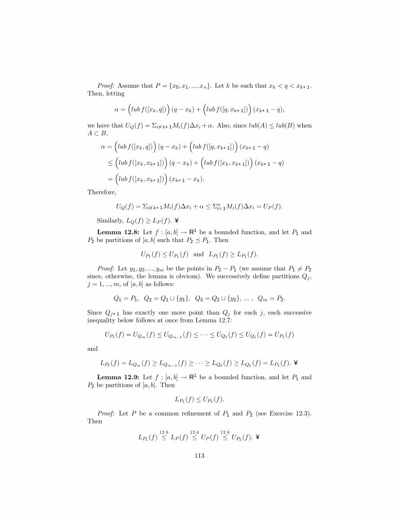
Proof: Assume that P = {x0, x1, ..., xn}. Let k be such that xk < q < xk+1.Then, letting

α =³lub f([xk, q])

´(q − xk) +

³lub f([q, xk+1])

´(xk+1 − q),

we have that UQ(f) = Σi 6=k+1Mi(f)∆xi+α. Also, since lub(A) ≤ lub(B) whenA ⊂ B,

α =³lub f([xk, q])

´(q − xk) +

³lub f([q, xk+1])

´(xk+1 − q)

≤³lub f([xk, xk+1])

´(q − xk) +

³lub f([xk, xk+1])

´(xk+1 − q)

=³lub f([xk, xk+1])

´(xk+1 − xk).

Therefore,

UQ(f) = Σi6=k+1Mi(f)∆xi + α ≤ Σni=1Mi(f)∆xi = UP (f).

Similarly, LQ(f) ≥ LP (f). ¥Lemma 12.8: Let f : [a, b] → R1 be a bounded function, and let P1 and

P2 be partitions of [a, b] such that P2 ¹ P1. Then

UP2(f) ≤ UP1

(f) and LP2(f) ≥ LP1

(f).

Proof: Let y1, y2, ..., ym be the points in P2 − P1 (we assume that P1 6= P2

since, otherwise, the lemma is obvious). We successively deÞne partitions Qj ,j = 1, ...,m, of [a, b] as follows:

Q1 = P1, Q2 = Q1 ∪ {y1}, Q3 = Q2 ∪ {y2}, ... , Qm = P2.

Since Qj+1 has exactly one more point than Qj for each j, each successiveinequality below follows at once from Lemma 12.7:

UP2(f) = UQm(f) ≤ UQm−1(f) ≤ · · · ≤ UQ2(f) ≤ UQ1(f) = UP1(f)

and

LP2(f) = LQm(f) ≥ LQm−1(f) ≥ · · · ≥ LQ2(f) ≥ LQ1(f) = LP1(f). ¥

Lemma 12.9: Let f : [a, b] → R1 be a bounded function, and let P1 andP2 be partitions of [a, b]. Then

LP1(f) ≤ UP2(f).

Proof: Let P be a common reÞnement of P1 and P2 (see Exercise 12.3).Then

LP1(f)12.8≤ LP (f)

12.6≤ UP (f)12.8≤ UP2(f). ¥

113

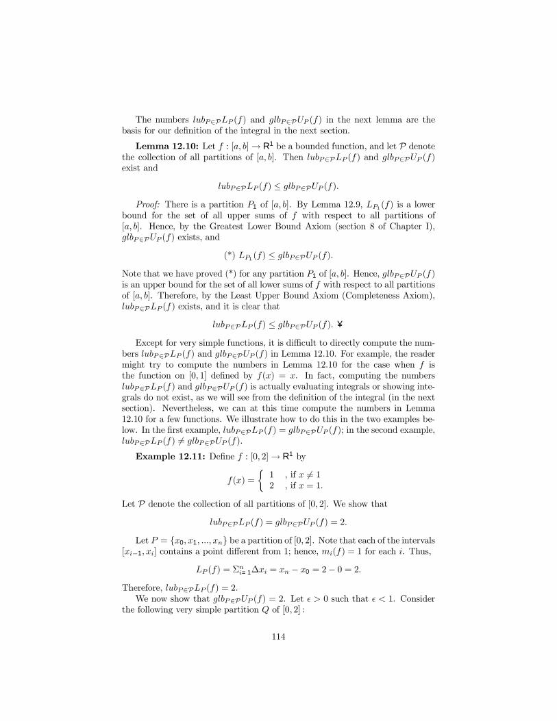
The numbers lubP∈PLP (f) and glbP∈PUP (f) in the next lemma are thebasis for our deÞnition of the integral in the next section.

Lemma 12.10: Let f : [a, b]→ R1 be a bounded function, and let P denotethe collection of all partitions of [a, b]. Then lubP∈PLP (f) and glbP∈PUP (f)exist and

lubP∈PLP (f) ≤ glbP∈PUP (f).Proof: There is a partition P1 of [a, b]. By Lemma 12.9, LP1

(f) is a lowerbound for the set of all upper sums of f with respect to all partitions of[a, b]. Hence, by the Greatest Lower Bound Axiom (section 8 of Chapter I),glbP∈PUP (f) exists, and

(*) LP1(f) ≤ glbP∈PUP (f).

Note that we have proved (*) for any partition P1 of [a, b]. Hence, glbP∈PUP (f)is an upper bound for the set of all lower sums of f with respect to all partitionsof [a, b]. Therefore, by the Least Upper Bound Axiom (Completeness Axiom),lubP∈PLP (f) exists, and it is clear that

lubP∈PLP (f) ≤ glbP∈PUP (f). ¥

Except for very simple functions, it is difficult to directly compute the num-bers lubP∈PLP (f) and glbP∈PUP (f) in Lemma 12.10. For example, the readermight try to compute the numbers in Lemma 12.10 for the case when f isthe function on [0, 1] deÞned by f(x) = x. In fact, computing the numberslubP∈PLP (f) and glbP∈PUP (f) is actually evaluating integrals or showing inte-grals do not exist, as we will see from the deÞnition of the integral (in the nextsection). Nevertheless, we can at this time compute the numbers in Lemma12.10 for a few functions. We illustrate how to do this in the two examples be-low. In the Þrst example, lubP∈PLP (f) = glbP∈PUP (f); in the second example,lubP∈PLP (f) 6= glbP∈PUP (f).Example 12.11: DeÞne f : [0, 2]→ R1 by

f(x) =

½1 , if x 6= 12 , if x = 1.

Let P denote the collection of all partitions of [0, 2]. We show thatlubP∈PLP (f) = glbP∈PUP (f) = 2.

Let P = {x0, x1, ..., xn} be a partition of [0, 2]. Note that each of the intervals[xi−1, xi] contains a point different from 1; hence, mi(f) = 1 for each i. Thus,

LP (f) = Σni=1∆xi = xn − x0 = 2− 0 = 2.

Therefore, lubP∈PLP (f) = 2.We now show that glbP∈PUP (f) = 2. Let ² > 0 such that ² < 1. Consider

the following very simple partition Q of [0, 2] :

114

Q = {0, 1− ², 1 + ², 2}.

We compute UQ(f) :

UQ(f) = 1([1− ²]− 0) + 2([1 + ²]− [1− ²]) + 1(2− [1 + ²]) = 2 + 2².

Thus, since ² can be as close to zero as we like, we have proved that

glbP∈PUP (f) ≤ 2.

Also, having proved above that lubP∈PLP (f) = 2, we know from Lemma 12.10that 2 ≤ glbP∈PUP (f). Therefore,

glbP∈PUP (f) = 2 = lubP∈PLP (f).

Example 12.12: DeÞne f : [0, 1]→ R1 by

f(x) =

½0 , if x is rational1 , if x is irrational.

Let P denote the collection of all partitions of [0, 1]. We show thatlubP∈PLP (f) = 0 and glbP∈PUP (f) = 1.

Let P = {x0, x1, ..., xn} be a partition of [0, 1]. By Theorem 1.26 (and itsanalogue for irrational numbers), there is a rational number and an irrationalnumber in each of the intervals [xi−1, xi]. Hence,

LP (f) = Σni=1(0)∆xi = 0

and

UP (f) = Σni=1(1)∆xi = (x1 − x0) + (x2 − x1) + · · ·+ (xn − xn−1)

= xn − x0 = 1− 0 = 1.Therefore, lubP∈PLP (f) = 0 and glbP∈PUP (f) = 1.

The cancellation that gave Σni=1∆xi = xn−x0 in Example 12.12 is trivial buthas far - reaching generalizations in multi - dimensional calculus (for example, inthe proof of Green�s Theorem).

Exercise 12.13: Let f be a constant function on an interval [a, b], sayf(x) = c for all x ∈ [a, b]. Compute lubP∈PLP (f) and glbP∈PUP (f).Exercise 12.14: DeÞne f : [0, 2]→ R1 by

f(x) =

½1 , if 0 ≤ x < 13 , if 1 ≤ x ≤ 2.

Compute lubP∈PLP (f) and glbP∈PUP (f).

115

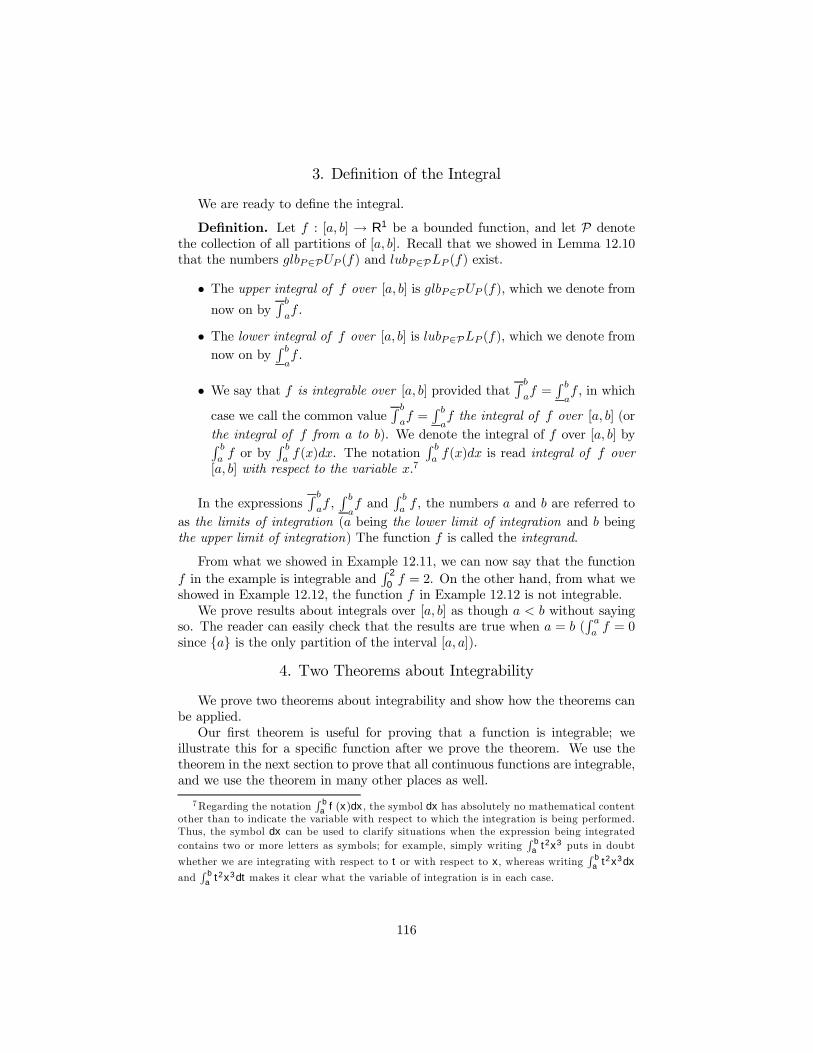
3. DeÞnition of the Integral

We are ready to deÞne the integral.

DeÞnition. Let f : [a, b] → R1 be a bounded function, and let P denotethe collection of all partitions of [a, b]. Recall that we showed in Lemma 12.10that the numbers glbP∈PUP (f) and lubP∈PLP (f) exist.

� The upper integral of f over [a, b] is glbP∈PUP (f), which we denote fromnow on by

R baf .

� The lower integral of f over [a, b] is lubP∈PLP (f), which we denote fromnow on by

R baf .

� We say that f is integrable over [a, b] provided that R baf =

R baf , in which

case we call the common valueR baf =

R baf the integral of f over [a, b] (or

the integral of f from a to b). We denote the integral of f over [a, b] byR ba f or by

R ba f(x)dx. The notation

R ba f(x)dx is read integral of f over

[a, b] with respect to the variable x.7

In the expressionsR baf ,

R baf and

R ba f , the numbers a and b are referred to

as the limits of integration (a being the lower limit of integration and b beingthe upper limit of integration) The function f is called the integrand.

From what we showed in Example 12.11, we can now say that the functionf in the example is integrable and

R 2

0 f = 2. On the other hand, from what weshowed in Example 12.12, the function f in Example 12.12 is not integrable.We prove results about integrals over [a, b] as though a < b without saying

so. The reader can easily check that the results are true when a = b (R aaf = 0

since {a} is the only partition of the interval [a, a]).

4. Two Theorems about Integrability

We prove two theorems about integrability and show how the theorems canbe applied.Our Þrst theorem is useful for proving that a function is integrable; we

illustrate this for a speciÞc function after we prove the theorem. We use thetheorem in the next section to prove that all continuous functions are integrable,and we use the theorem in many other places as well.

7Regarding the notationR b

a f(x)dx, the symbol dx has absolutely no mathematical contentother than to indicate the variable with respect to which the integration is being performed.Thus, the symbol dx can be used to clarify situations when the expression being integratedcontains two or more letters as symbols; for example, simply writing

R ba

t2x3 puts in doubt

whether we are integrating with respect to t or with respect to x, whereas writingR b

a t2x3dx

andR b

at2x3dt makes it clear what the variable of integration is in each case.

116

Theorem 12.15: Let f : [a, b] → R1 be a bounded function. Then f isintegrable over [a, b] if and only if for each ² > 0, there is a partition P of [a, b]such that

UP (f)− LP (f) < ².Proof: Assume that f is integrable over [a, b]. Let ² > 0. SinceR b

af =

R baf = glbP∈PUP (f) and

R baf =

R baf = lubP∈PLP (f),

there are a partitions P1 and P2 of [a, b] such that

(1) UP1(f) <

R ba f +

²2 and LP2

(f) >R ba f − ²

2 .

Let P be a common reÞnement of P1 and P2 (see Exercise 12.3). Then, byLemma 12.6 and Lemma 12.8 , we have

(2) LP2(f) ≤ LP (f) ≤ UP (f) ≤ UP1(f).

Now,

UP (f)− LP (f)(2)≤ UP1

(f)− LP2(f)

(1)<R ba f +

²2 − (

R ba f − ²

2) = ².

This proves that P is as required in the theorem.Conversely, assume that for each ² > 0, there is a partition P² of [a, b] such

that

UP²(f)− LP²(f) < ².

Then, sinceR baf = glbP∈PUP (f) and

R baf = lubP∈PLP (f),

012.10≤ R b

af −R baf ≤ UP²(f)− LP²(f) < ² for all ² > 0.

Hence,R baf −R b

af = 0 (it follows from the axioms in section 1 of Chapter I that

if 0 ≤ x < ² for all ² > 0, then x = 0). Therefore,R baf =

R baf , which proves

that f is integrable. ¥Lest it escape us without notice, we point out that Theorem 12.15 says that

we need only Þnd one appropriate partition for each ² > 0 in order to showa function is integrable. This feature of Theorem 12.15 makes it signiÞcantlyeasier to show a function is integrable than it would be to show the function isintegrable using the deÞnition of integrability directly. We illustrate this withthe following example:

Example 12.16: DeÞne f : [0, 2] → R1 by f(x) = x2. We show that f isintegrable over [0, 2] by applying Theorem 12.15.Let ² > 0. Let n be a natural number such that 4

n < ² (the number n existsby the Archimedean Property (Theorem 1.22)). Let P be the partition of [0, 2]given by

117

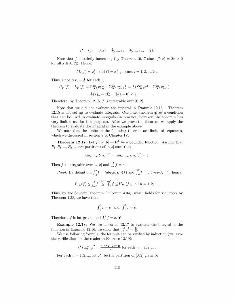
P = {x0 = 0, x1 =1n , ..., xi =

in , ..., x2n = 2}.

Note that f is strictly increasing (by Theorem 10.17 since f 0(x) = 2x > 0for all x ∈ [0, 2]). Hence,

Mi(f) = x2i , mi(f) = x

2i−1, each i = 1, 2, ..., 2n.

Thus, since ∆xi = 1n for each i,

UP (f)− LP (f) = Σ2ni=1x

2i

1n −Σ2n

i=1x2i−1

1n =

1n(Σ

2ni=1x

2i −Σ2n

i=1x2i−1)

= 1n(x

22n − x2

0) =1n(4− 0) < ².

Therefore, by Theorem 12.15, f is integrable over [0, 2].

Note that we did not evaluate the integral in Example 12.16 � Theorem12.15 is not set up to evaluate integrals. Our next theorem gives a conditionthat can be used to evaluate integrals (in practice, however, the theorem hasvery limited use for this purpose). After we prove the theorem, we apply thetheorem to evaluate the integral in the example above.We note that the limits in the following theorem are limits of sequences,

which we discussed in section 8 of Chapter IV.

Theorem 12.17: Let f : [a, b] → R1 be a bounded function. Assume thatP1, P2, ..., Pn, ... are partitions of [a, b] such that

limn→∞UPn(f) = limn→∞LPn(f) = c.

Then f is integrable over [a, b] andR ba f = c.

Proof: By deÞnition,R baf = lubP∈PLP (f) and

R baf = glbP∈PUP (f); hence,

LPn(f) ≤R baf12.10≤ R b

af ≤ UPn(f), all n = 1, 2, ... .

Thus, by the Squeeze Theorem (Theorem 4.34), which holds for sequences byTheorem 4.38, we have thatR b

af = c and

R baf = c.

Therefore, f is integrable andR ba f = c. ¥

Example 12.18: We use Theorem 12.17 to evaluate the integral of thefunction in Example 12.16; we show that

R 2

0x2 = 8

3 .We use following formula; the formula can be veriÞed by induction (we leave

the veriÞcation for the reader in Exercise 12.19):

(*) Σni=1i2 = n(n+1)(2n+1)

6 for each n = 1, 2, ... .

For each n = 1, 2, ..., let Pn be the partition of [0, 2] given by

118

Pn = {x0 = 0, x1 =1n , ..., xi =

in , ..., x2n = 2}.

Then, since Mi(f) = x2i and mi(f) = x

2i−1 for each i (as in Example 12.16),

UPn(f) = Σ2ni=1x

2i

1n and LPn(f) = Σ

2ni=1x

2i−1

1n for each n.

Hence, for each n,

UPn(f) =1nΣ

2ni=1(

in)

2 = 1n3Σ2n

i=1i2 (*)= 1

n32n(2n+1)(4n+1)

6

= (2n+1)(4n+1)3n2 = 8

3 +2n +

13n2

and

LPn(f) = Σ2ni=1(

i−1n )

2 1n =

1n3Σ

2ni=1(i− 1)2 = 1

n3Σ2n−1i=1 i2

(*)= 1

n3

(2n−1)(2n)(4n−1)6 = (2n−1)(4n−1)

3n2 = 83 − 2

n +1

3n2 .

Thus, limn→∞UPn(f) =83 and limn→∞LPn(f) =

83 . Therefore, by Theorem

12.17,R 2

0 x2 = 8

3 .

Exercise 12.19: Verify that Σni=1i2 = n(n+1)(2n+1)

6 for each n = 1, 2, ... byusing induction (Theorem 1.20). (We used the formula in Example 12.18.)

In Examples 12.16 and 12.18, we used partitions that divide the interval ofintegration into intervals of equal length. These types of partitions are usefulbecause we can factor ∆xi out of summations when computing upper and lowersums. We call a partition of an interval [a, b] that divides [a, b] into intervals ofequal length ∆xi a regular partition.

Exercise 12.20: EvaluateR ba x for any a ≤ b.

(Hint: First prove that Σni=1i =n(n+1)

2 for each n = 1, 2, ... .)

Exercise 12.21: Determine if f is integrable, where f : [0, 1] → R1 isdeÞned as follows (Q denotes the set of all rational numbers; for integers m andn, mn in lowest terms means m and n have no common divisor other than ±1):

f(x) =

0 , if x is irrational

1 , if x = 01n , if x ∈ Q− {0} and x = m

n in lowest terms.

Exercise 12.22: Assume that f(x) ≤ g(x) ≤ h(x) for all x ∈ [a, b] and thatf and h are integrable over [a, b]. If

R baf =

R bah, then g is integrable and

R bag

is equal toR ba f =

R ba h.

Exercise 12.23: If f is increasing on [a, b] or decreasing on [a, b], then f isintegrable over [a, b].

Exercise 12.24: In connection with Exercise 12.23, is every one - to - onebounded function on an interval [a, b] integrable over [a, b] ?

119

Exercise 12.25: If f : [a, b] → R1 is a nonnegative function that is inte-grable over [a, b], then

R ba f ≥ 0.

Exercise 12.26: Let f : [a, b] → R1 be a nonnegative function that isintegrable over [a, b]. Then

R baf = 0 if and only if glbf(I) = 0 for each open

interval I in [a, b].

Exercise 12.27: Let f : [a, b] → R1 be a function that is integrable over[a, b], and let g : [a, b]→ R1 be a function that agrees with f except at Þnitelymany points. Is g integrable over [a, b] ?

5. Continuous Functions Are Integrable

We prove that any continuous function deÞned on a closed and boundedinterval is integrable. This is an existence theorem � it does not show how toevaluate the integral. We will be able to evaluate integrals of many simple con-tinuous functions using the Fundamental Theorem of Calculus, which we provein Chapter XIV. However, evaluating integrals of most continuous functions isdifficult, usually impossible; ad hoc methods can sometimes be employed, butmost often one has to settle for approximate evaluations by numerical methods.The following notion is of general importance and is the key idea that we

use to prove our theorem:

DeÞnition: Let X ⊂ R1, and let f : X → R1 be a function. We say that fis uniformly continuous on X provided that for any ² > 0, there is a δ > 0 suchthat if x1, x2 ∈ X and |x1 − x2| < δ, then |f(x1)− f(x2)| < ².Exercise 12.28: Let X ⊂ R1. If f : X → R1 is uniformly continuous, then

f is continuous.

Exercise 12.29: The converse of the result in Exercise 12.28 is false: Thefunction f : R1 → R1 given by f(x) = x2 is continuous but not uniformlycontinuous.

Exercise 12.30: Any linear function f (i.e., f(x) = mx + b) is uniformlycontinuous on R1. More generally, if f is differentiable on an interval I and thederivative f 0 is bounded on I, then f is uniformly continuous on I.

The following theorem is not concerned with integrals, but it is the basis ofour proof that continuous functions are integrable. The theorem is so importantin all of mathematics that even though it plays the role of a lemma here, we cannot bring ourselves to call the theorem a lemma. The theorem shows that theconverse of the result in Exercise 12.28 is true when X is a closed and boundedinterval.

Theorem 12.31: If f : [a, b] → R1 is continuous, then f is uniformlycontinuous.

Proof: Suppose by way of contradiction that f is not uniformly continuous.Then, for some ² > 0, there are points xn, yn ∈ [a, b] for each n ∈ N such that

120