5 chapter 14: partial derivatives. 5.1 functions of several variables ⇤...

Multivariate Calculus; Fall 2013 S. Jamshidi

5 Chapter 14: Partial Derivatives

In the previous chapter, we studied vector functions

~r(t) = hf(t), g(t), h(t)i

which took in a scalar t and spit out a vector ~r(t). In this chapter, we will study functions thattake in multiple scalar inputs, like x and y, but produce just one scalar output

z = f(x, y).

These are called functions of several variables. They are the main object of study in multivariatecalculus.

5.1 Functions of Several Variables

⇤ I know how to find the domain of a function of several variables. If there are twoor three input variables, I know how to graph the domain.

⇤ I know how to find the range of a function of several variables. I can graph it.

⇤ I know how to graph level curves when there are two input variables.

Objectives

The first step in understanding any function is being able to recognize its domain and range.

Definition 5.1.1 The domain, D, of a function of many variables, like f(x, y), is the set of valuesf takes in. It’s range, R, is the set of values f spits out.

While this sounds simple, in practice we have to consider situations we didn’t in two-dimensionalcalculus. Namely, we have to think about the variables individually and together.

Here are some things to keep in mind when you are doing this problems:

• The range will always be one-dimensional.

• The domain will have the same number of dimensions as there are input variables.

• The domain needs to include *all* possible inputs, which can make graphing it very tricky.

95 of 146


5.1.1 Examples

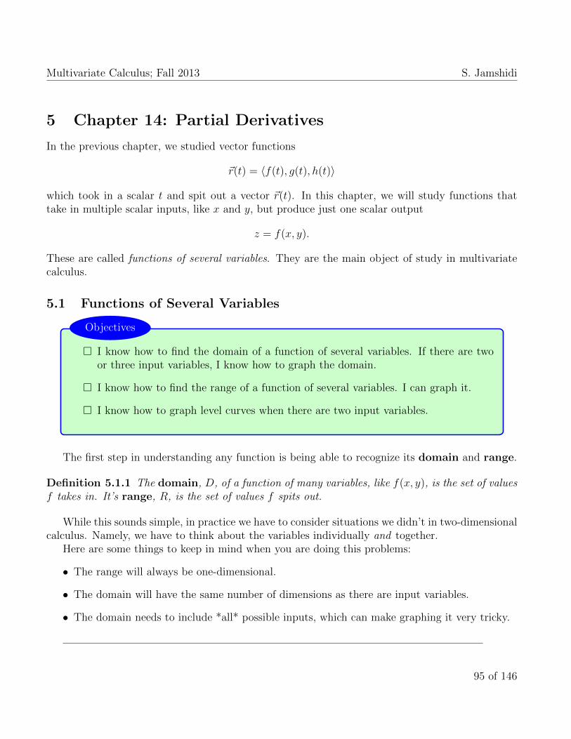
Example 5.1.1.1 For the function below, find and sketch the domain then find its range.

f(x, y) =px+ y

Any value under the square root must be greater than or equal to zero. Therefore, the domainis

D = {(x, y) | x+ y � 0}Surely if both x and y are positive numbers, then x+y � 0. But, is that enough? What if x = 4

and y = �2. Their sum is then 2, which is greater than 0. How to we account for cases like this?This might not be obvious. To help us figure this out, we’ll think about the extreme cases. That

would be x = �y and y = �x. These are cases like (x, y) = (�4, 4) or (x, y) = (2,�2). Both ofthese cases correspond to the same line: y = �x. Everything above this line will satisfy the domainrestriction. Check a few points to convince yourself.

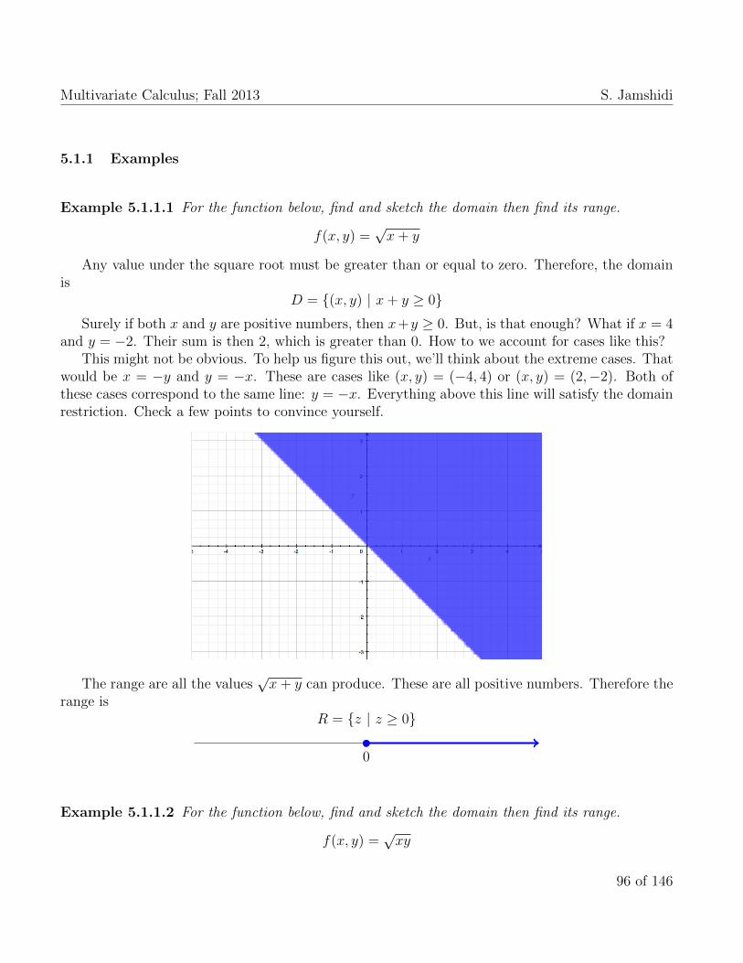
The range are all the valuespx+ y can produce. These are all positive numbers. Therefore the

range isR = {z | z � 0}

0

Example 5.1.1.2 For the function below, find and sketch the domain then find its range.

f(x, y) =pxy

96 of 146


As before, any value under the square root must be greater than or equal to zero. As a result, ourdomain is

D = {(x, y) | xy � 0}

How do we graph this? If xy � 0, then we’re looking at two regions.

1. x � 0 and y � 0

2. x 0 and y 0 (remember, the product of two negative numbers is positive!)

The range are all the valuespxy spits out. It can only be number greater than or equal to zero.

So we haveR = {z | z � 0}

0

Example 5.1.1.3 For the function below, find its domain and graph it.

f(x, y, z) = ln(16� 4x2 � 4y2 � z

2)

Then, find its range.

Values inside ln() must be strictly positive, so the domain is

D = {(x, y, z) | 16� 4x2 � 4y2 � z

2> 0}.

But is this really the best way to express this set? It doesn’t tell us anything in this form. So, let’stry to simplify the expression a little.

97 of 146


16� 4x2 � 4y2 � z

2> 0

16 > 4x2 + 4y2 + z

2

4 > x

2 + y

2 +z

2

4

The graph of the domain is then a solid ellipse but missing its shell.

The natural log (ln) takes in only positive values, but produces all real numbers. Rememberthat the natural log of numbers between 0 and 1 are negative. So the range is

R = {z | z 2 R} = {z | all real numbers}

Either expression is an acceptable answer.Here is the graph of the range.

0

In addition to looking at the domain and range, we want to be able to graph functions in threedimensions. This is quite tricky. One popular method is to graph level curves. These are the linesone sees on a topographic map. Below is an example of a topographic map of Tussey Mountain.

98 of 146


Notice the lines looping around with jagged edges. Around the word “FRANKLIN,” we see aloop labeled 1300. This tells us that on that line, the elevation is 1300ft.

Level curves are a way to think about f as a height. What we’ll do is pick values for f andgraph the resulting two-dimensional curve. This process won’t be useful if you have more than twoinput variables.

99 of 146


5.1.2 Examples

Example 5.1.2.1 Graph the level curves of

f(x, y) =px+ y

Use that information to sketch the 3 dimensional graph.

Let’s pick values for f and write the respective functions.

f Function

0 0 =px+ y =) 0 = x+ y

1 1 =px+ y =) 1 = x+ y

2 2 =px+ y =) 4 = x+ y

3 3 =px+ y =) 9 = x+ y

Now, we graph all these lines on the same graph.

100 of 146


From this, we see that the curve is increasing in height but the increasing is slowing down. Hereis the graph of the three dimensional surface seen from two di↵erent angles.

Example 5.1.2.2 Graph the level curves of

f(x, y) =pxy

Use that information to sketch the 3 dimensional graph.

First, we pick z values. In the picture below, I have graphed z = 1, z = 2, ..., and z = 7.

f Function

0 0 =pxy

1 1 =pxy

2 2 =pxy

3 3 =pxy

4 4 =pxy

5 5 =pxy

6 6 =pxy

101 of 146


Given the shape of the level curve, our graph is then

102 of 146


• The domain is a set of inputs that are valid for the function.

• The range is all the values produced by the function. It will always be one-dimensional for functions of multiple variables.

• The level curves are the lines for various values of the function, f .

• Drawing level curves is a technique for graphing three-dimensional surfaces.

Summary of Ideas: Functions of Several Variables

103 of 146

5 chapter 14: partial derivatives. 5.1 functions of several variables ⇤...

Documents