4working with formulas · basic formulas and functions in excel. formulas are one of excel’s most...
TRANSCRIPT

In this lesson, you will create and modify basic formulas and functions in Excel. Formulas are one of Excel’s most powerful
features, as they can save you time and increase the accuracy of your spreadsheets. You will reference cells in formulas and use AutoSum. Lastly, you will use IF functions, which can flag a cell with a text label, display a value, or perform a calculation when specific criteria are satisfied.
L E S S O N O U T L I N EWorking with Formulas and FunctionsCreating FormulasUsing Cell References in FormulasModifying and Copying FormulasDisplaying and Printing FormulasUsing Formula AutoCompleteUsing Insert FunctionCreating Formulas with the IF FunctionConcepts ReviewReinforce Your Skills
Apply Your Skills
Extend Your Skills
Transfer Your Skills
L E A R N I N G O B J E C T I V E SAfter studying this lesson, you will be able to:
■■ Create formulas to calculate values
■■ Use functions such as sum, average, maximum, minimum, and IF
■■ Use relative, absolute, and mixed cell references in formulas
■■ Modify and copy formulas
■■ Display formulas rather than resulting values in cells
4Working with Formulas and Functions
E X C E L 2 0 1 3
Lessons from Microsoft Office 2013 FOR EVALUATION ONLY (c) 2014 Labyrinth Learning - Not for Sale or Classroom Use
Labyrinth Learning http://www.lablearning.com
EVALUATIO
N ONLY

C A S E S T U D Y
EX04.2
C A S E S T U D Y
Creating a Spreadsheet with FormulasGreen Clean earns revenue by selling janitorial products and contracts for cleaning services. You want to set up a workbook with two worksheets, one to track commissions and the other to report how the projected profit would change based on costs and an increase or decrease in sales.
This worksheet sums the monthly totals for all team members as well as the quarterly sales for each.
This worksheet reports the effect of various sales projections and costs on net profit.
Lessons from Microsoft Office 2013 FOR EVALUATION ONLY (c) 2014 Labyrinth Learning - Not for Sale or Classroom Use
Labyrinth Learning http://www.lablearning.com
EVALUATIO
N ONLY

Working with Formulas and Functions EX04.3
Exce
l 201
3
Working with Formulas and FunctionsVideo Library http://labyrinthelab.com/videos Video Number: EX13-V0401
A formula is a math problem done in Excel. You can add, subtract, multiply, divide, and group cell contents to make your data work for you. A function is a prewritten formula that can simplify complex procedures for numbers and text. For instance, a function can be used to sum a group of numbers, to determine the payment amount on a loan, and to convert a number to text.
Using AutoSum to Create a SUM FormulaThe AutoSum button automatically sums a column or row of numbers. When you click AutoSum, Excel starts the formula for you by entering =SUM() and proposes a range of adjacent cells within the parentheses. Excel first looks upward for a range to sum. If a range is not found there, it next looks left. You can accept the proposed range, which can be viewed in the Formula Bar, or drag in the worksheet to select a different range.
The Formula Bar displays the formula.
Excel proposes to sum the range B5:B8 and adds a flashing marquee.
The formula is being created in cell B9.
The result displays after you confirm the formula.
Average, Count, CountA, Max, and Min FunctionsIn addition to summing a group of numbers, the AutoSum button can perform a number of other calculations.
AutoSum and/or Status Bar Function
How Function Appears in Formula
Description
Sum SUM Adds the values in the cells
Average AVERAGE Averages the values in the cells
Count Numbers or Numerical Count
COUNT Counts the number of values in the cells; cells containing text and blank cells are ignored
Count COUNTA Counts the number of nonblank cells
Max or Maximum MAX Returns the highest value in the cells
Min or Minimum MIN Returns the lowest value in the cells
FROM THE RIBBON
Home→Editing →AutoSum
FROM THE KEYBOARD[Alt] + [=]
Lessons from Microsoft Office 2013 FOR EVALUATION ONLY (c) 2014 Labyrinth Learning - Not for Sale or Classroom Use
Labyrinth Learning http://www.lablearning.com
EVALUATIO
N ONLY

EX04.4 Excel 2013 Lesson 4: Working with Formulas and Functions
TIP
Once you have entered a formula in a cell, you can use AutoFill to copy it to adjacent cells.
Status Bar FunctionsThe Status Bar, which is displayed at the bottom of the Excel window, can be customized to display a variety of functions including Average, Count, Numerical Count, Minimum, Maximum, and Sum. To customize the Status Bar, right-click anywhere on it and click to add or remove features. You can also customize additional features of the Status Bar, such as Zoom, Signatures, Overtype Mode, and Macro Recording.
By default, Excel displays in the Status Bar the average, count of values, and sum of the selected range.
QUICK REFERENCE USING AUTOSUM AND THE STATUS BAR FUNCTIONS
Task Procedure
AutoSum a range of cells
■■ Click in the desired cell and choose Home→Editing→AutoSum .
■■ Tap [Enter] to confirm the proposed range, or drag to select the correct range and tap [Enter].
AutoSum across columns or down rows
■■ Select the cell in the row directly below or column directly to the right of the data where you want the sums to appear and choose Home→Editing→AutoSum .
Use Status Bar functions
■■ Right-click the Status Bar and add or remove the desired functions.
■■ Select the desired range, and view the results of the desired functions within the Status Bar.
Lessons from Microsoft Office 2013 FOR EVALUATION ONLY (c) 2014 Labyrinth Learning - Not for Sale or Classroom Use
Labyrinth Learning http://www.lablearning.com
EVALUATIO
N ONLY

Working with Formulas and Functions EX04.5
Exce
l 201
3
DEVELOP YOUR SKILLS EX04-D01
Use AutoSum and Status Bar Functions In this exercise, you will use AutoSum to calculate the monthly commission total for the sales team as well as the quarterly total for each sales team member.
1. Open EX04-D01-Commissions from the Excel 2013 Lesson 04 folder, and save it as EX04-D01-Commissions-FirstInitialLastName.
Replace the bracketed text with your first initial and last name. For example, if your name is Bethany Smith, your filename would look like this: EX04-D01-Commissions-BSmith. Notice the two tabs at the bottom of the window: Qtr 1 Commissions and Profit Projection.
2. With the Qtr 1 Commissions worksheet displayed, select cell B9.
3. Choose Home→Editing→AutoSum .
Excel displays a marquee around the part of the spreadsheet where it thinks the formula should be applied. You can change this selection as necessary.
4. Follow these steps to complete the Sum formula:
Click Enter to complete the entry. The total should be 1059.
Note the proposed formula, a sum of numbers in the range B5:B8.
Notice that AutoSum adds a flashing marquee around the range B5:B8, the most likely range for the formula.
5. Select cell E7 and choose Home→Editing→AutoSum .
Notice that, as there are no values above cell E7, Excel looked to the left to find a range to sum, B7:D7. Now, assume that you wanted only cells B7:C7 to be summed.
6. Follow these steps to override the proposed range:
Select the range B7:C7.
Notice that the new range, B7:C7, appears in the formula.
Tap [Enter] to complete the formula.
7. Undo the formula.
Lessons from Microsoft Office 2013 FOR EVALUATION ONLY (c) 2014 Labyrinth Learning - Not for Sale or Classroom Use
Labyrinth Learning http://www.lablearning.com
EVALUATIO
N ONLY

EX04.6 Excel 2013 Lesson 4: Working with Formulas and Functions
Use AutoFill to Extend a Formula
8. Follow these steps to AutoFill the formula in cell B9 into the cells to its right:
Select cell B9. Position the mouse pointer over the fill handle at the bottom-right corner of the cell and drag to cell E9.
Release the mouse button to fill the formula into the cells.
Cell E9 displays 0 because the cells above it are empty. You can create formulas that include empty cells and then enter data later.
9. Select the range E5:E8.
10. Choose Home→Editing→AutoSum to calculate the quarterly totals.
Excel created a formula in each cell of the selected range without requiring you to complete the formulas.
11. Delete the formulas in range B9:E9 and range E5:E8.
The data are returned to their original state.
12. Select the range B5:E9 and click AutoSum .
The formula results appear in B9:E9 and E5:E8.
Explore Statistical Functions with AutoSum
13. Select cell B11.
14. Choose Home→Editing→AutoSum menu button.
15. Choose Average from the drop-down menu.
Excel proposes the range B5:B10, which is incorrect.
16. Select the correct range B5:B8 and tap [Enter] to complete the entry.
The result should equal 264.75.
17. With cell B12 selected, choose Home→Editing→AutoSum menu button→Max.
18. Select the correct range B5:B8 and tap [Enter] to display the highest value in the range.
The result should equal 389.
19. Select cell B13 and choose Home→Editing→AutoSum menu button→Min.
Min represents Minimum, or the lowest value.
Lessons from Microsoft Office 2013 FOR EVALUATION ONLY (c) 2014 Labyrinth Learning - Not for Sale or Classroom Use
Labyrinth Learning http://www.lablearning.com
EVALUATIO
N ONLY

Creating Formulas EX04.7
Exce
l 201
3
20. Correct the range to B5:B8 and then click Enter on the Formula Bar to display the lowest value in the range.
The result should equal 74.
21. Select cell B14 and choose Home→Editing→AutoSum menu button.
22. Choose Count Numbers, correct the range to B5:B8, and click Enter .
23. Select cell B6 and delete the contents.
The formula recalculates the count as 3, and both the average and minimum formulas recalculate as well.
24. Undo the deletion.
Use Status Bar Functions
25. Select the range B5:B8.
26. Look at the Status Bar in the lower-right corner of the window to see that the sum value displayed equals the result in cell B9. Save the workbook and leave it open.
Creating FormulasVideo Library http://labyrinthelab.com/videos Video Number: EX13-V0402
As you saw with AutoSum, functions begin with an equals (=) sign. Formulas begin with an equals sign as well, although Excel will automatically insert the equals sign if you first type a plus (+) or a minus (–) sign.
Cell and Range ReferencesFormulas derive their power from the use of cell and range references. Using references in formulas ensures that formulas can be copied to other cells and that results are automatically recalculated when the data is changed in the referenced cell(s).
WARNING
Do not type the results of calculations directly into cells. Always use formulas.
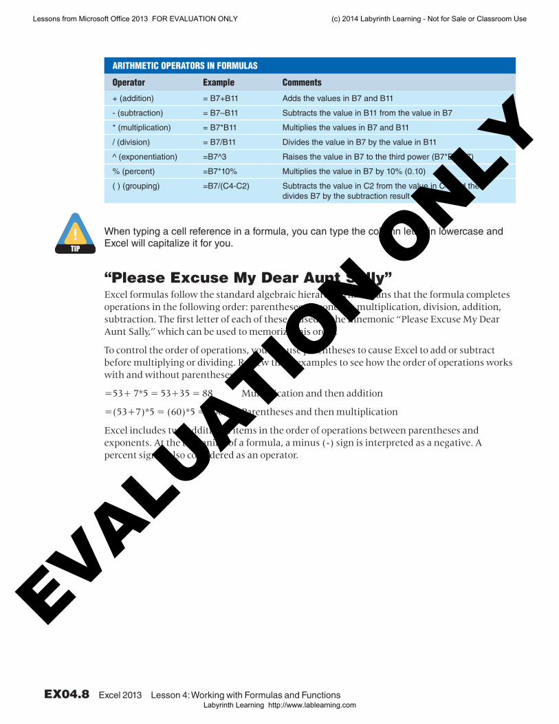
The Language of Excel FormulasFormulas can include the standard arithmetic operators shown in the following table. Keep in mind that each formula you create will be entered into the same cell that displays the resulting calculation.
Lessons from Microsoft Office 2013 FOR EVALUATION ONLY (c) 2014 Labyrinth Learning - Not for Sale or Classroom Use
Labyrinth Learning http://www.lablearning.com
EVALUATIO
N ONLY
EX04.8 Excel 2013 Lesson 4: Working with Formulas and Functions
ARITHMETIC OPERATORS IN FORMULAS
Operator Example Comments
+ (addition) = B7+B11 Adds the values in B7 and B11
- (subtraction) = B7–B11 Subtracts the value in B11 from the value in B7
* (multiplication) = B7*B11 Multiplies the values in B7 and B11
/ (division) = B7/B11 Divides the value in B7 by the value in B11
^ (exponentiation) =B7^3 Raises the value in B7 to the third power (B7*B7*B7)
% (percent) =B7*10% Multiplies the value in B7 by 10% (0.10)
( ) (grouping) =B7/(C4-C2) Subtracts the value in C2 from the value in C4 and then divides B7 by the subtraction result
TIP
When typing a cell reference in a formula, you can type the column letter in lowercase and Excel will capitalize it for you.
“Please Excuse My Dear Aunt Sally”Excel formulas follow the standard algebraic hierarchy. This means that the formula completes operations in the following order: parentheses, exponents, multiplication, division, addition, subtraction. The first letter of each of these is used in the mnemonic “Please Excuse My Dear Aunt Sally,” which can be used to memorize this order.
To control the order of operations, you can use parentheses to cause Excel to add or subtract before multiplying or dividing. Review these examples to see how the order of operations works with and without parentheses.
=53+ 7*5 = 53+35 = 88 Multiplication and then addition
=(53+7)*5 = (60)*5 = 300 Parentheses and then multiplication
Excel includes two additional items in the order of operations between parentheses and exponents. At the beginning of a formula, a minus (-) sign is interpreted as a negative. A percent sign is also considered as an operator.
Lessons from Microsoft Office 2013 FOR EVALUATION ONLY (c) 2014 Labyrinth Learning - Not for Sale or Classroom Use
Labyrinth Learning http://www.lablearning.com
EVALUATIO
N ONLY

Using Cell References in Formulas EX04.9
Exce
l 201
3
DEVELOP YOUR SKILLS EX04-D02
Use the Keyboard to Create FormulasIn this exercise, you will use the keyboard to enter formulas into the spreadsheet.
1. Save your file as EX04-D02-Commissions-FirstInitialLastName.
2. Click the Profit Projection sheet tab at the bottom of the Excel window.
3. Select cell B5 and view its formula in the Formula Bar.
This formula multiplies the number of contracts (B17) by the average contract revenue (B18).
4. Select cell B6 and use AutoSum to sum the sales in the range B4:B5.
5. In cell B11, sum the costs in the range B8:B10.
The total costs result is not correct, but you will enter data in cells B9 and B10 in the next exercise.
6. Select cell B13, the Gross Profit for the Base column.
7. Type =B6-B11 in the cell, and then tap (Enter) to complete the formula.
In order to calculate the gross profit, you need to subtract the total costs (B11) from total revenue (B6).
8. Select cell B15, which is within the Gross Profit vs. Revenue row.
9. Type =b13/b6 in the cell, tap (Enter), and save the workbook.
In this worksheet, the cell has been formatted to display a percentage for you.
Using Cell References in FormulasVideo Library http://labyrinthelab.com/videos Video Number: EX13-V0403
A cell reference can be used to represent a cell or range of cells containing the values used in a formula. Cell references are one of three types: relative, absolute, or mixed.
Relative Cell References A relative cell reference is one where the location is relative to the cell that contains the formula. For example, when you enter the formula =A3-B3 in cell C3, Excel notes that cell A3 is two cells to the left of the formula and that cell B3 is one cell to the left of the formula. When you copy the formula, the cell references update automatically. So, if the formula were copied to cell C4, the new formula would be =A4-B4. Excel updates the cell references so they are the same distance from cell C4 as were the cell references in the original formula in cell C3.
Lessons from Microsoft Office 2013 FOR EVALUATION ONLY (c) 2014 Labyrinth Learning - Not for Sale or Classroom Use
Labyrinth Learning http://www.lablearning.com
EVALUATIO
N ONLY

EX04.10 Excel 2013 Lesson 4: Working with Formulas and Functions
Absolute Cell ReferencesIn some situations, you may not want references updated when a formula is moved or copied. You must use either absolute or mixed references in these situations. Absolute references within a formula always refer to the same cell, even when the formula is copied to another location. You create absolute references by placing dollar signs in front of the column and row components of the reference. For example, if the formula = $A$3-$B$3 were entered in cell C3, and then copied to cell C4, the formula within cell C4 would still read = $A$3-$B$3.
Mixed ReferencesYou can mix relative and absolute references. For example, the reference $C1 is a combination of an absolute reference to column C and a relative reference to row 1. This can be useful when copying a formula both across a row and down a column.
Using the [F4] Function KeyThe [F4] function key can be used to insert the dollar signs within a cell reference. When [F4] is first tapped, dollar signs are placed in front of the column and row components of the cell reference. A second tap of [F4] places a dollar sign in front of only the row component, a third tap places one sign in front of only the column component, and a fourth tap removes all dollar signs.
The following table indicates what happens to different types of cell references when their formulas are copied to other locations.
Cell Reference Type Copy and Paste Action Result When Pasted
B6 Relative One column to the right C6
B6 Relative One row down B7
$B$6 Absolute One column to the right $B$6
$B$6 Absolute One row down $B$6
$B6 Mixed One column to the right $B6
$B6 Mixed One row down $B7
B$6 Mixed One column to the right C$6
B$6 Mixed One row down B$6
Lessons from Microsoft Office 2013 FOR EVALUATION ONLY (c) 2014 Labyrinth Learning - Not for Sale or Classroom Use
Labyrinth Learning http://www.lablearning.com
EVALUATIO
N ONLY
Using Cell References in Formulas EX04.11
Exce
l 201
3
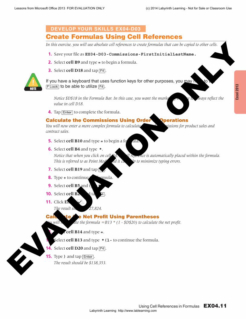
DEVELOP YOUR SKILLS EX04-D03
Create Formulas Using Cell ReferencesIn this exercise, you will use absolute cell references to create formulas that can be copied to other cells.
1. Save your file as EX04-D03-Commissions-FirstInitialLastName.
2. Select cell B9 and type = to begin a formula.
3. Select cell D18 and tap [F4].
NOTE
If you have a keyboard that uses function keys for other purposes, you may have to tap (F«Lock) to be able to utilize (F4).
Notice $D$18 in the Formula Bar. In this case, you want the marketing expense to always reflect the value in cell D18.
4. Tap [Enter] to complete the formula.
Calculate the Commissions Using Order of OperationsYou will now enter a more complex formula to calculate the total commissions for product sales and contract sales.
5. Select cell B10 and type = to begin a formula.
6. Select cell B4 and type *.
Notice that when you click on cell B4, its cell reference is automatically placed within the formula. This is referred to as Point Mode, and it can help to minimize typing errors.
7. Select cell B19 and tap [F4].
8. Type + to continue the formula.
9. Select cell B5 and type *.
10. Select cell B20 and tap [F4].
11. Click Enter .
The result should be 27,824.
Calculate the Net Profit Using ParenthesesYou will now create the formula =B13 * (1 - $D$20) to calculate the net profit.
12. Select cell B14 and type =.
13. Select cell B13 and type *(1- to continue the formula.
14. Select cell D20 and tap [F4].
15. Type ) and tap [Enter].
The result should be $138,353.
Lessons from Microsoft Office 2013 FOR EVALUATION ONLY (c) 2014 Labyrinth Learning - Not for Sale or Classroom Use
Labyrinth Learning http://www.lablearning.com
EVALUATIO
N ONLY

EX04.12 Excel 2013 Lesson 4: Working with Formulas and Functions
Project a Sales IncreaseYou will now create the formula =$B$4 * (1 + C$3) to project a 2 percent increase over the base product sales.
16. Select cell C4 and type an equals sign (=).
17. Select cell B4 and tap [F4].
18. Type *(1+ to continue the formula.
19. Select cell C3 and tap [F4] two times to create the C$3 mixed cell reference.
20. Type ) and tap [Enter].
The result should equal 54,264.
21. With cell C5 selected, repeat steps 16–20 (but using different cell references) to project a 2 percent increase for base contract sales.
The result should equal 245,820.
22. Save the workbook.
Modifying and Copying FormulasVideo Library http://labyrinthelab.com/videos Video Number: EX13-V0404
You can modify and copy formulas just like you edit and copy cells.
Modifying FormulasYou can edit a formula either in the Formula Bar or by double-clicking the formula cell. If you click or select a cell and enter a new formula, it replaces the previous contents.
When you select a formula to edit it, you will see colored lines around all cells referenced by the formula. This feature can help you track the formula elements.
Excel graphically displays the cells referenced by the formula, B13 and D20.
Lessons from Microsoft Office 2013 FOR EVALUATION ONLY (c) 2014 Labyrinth Learning - Not for Sale or Classroom Use
Labyrinth Learning http://www.lablearning.com
EVALUATIO
N ONLY
Modifying and Copying Formulas EX04.13
Exce
l 201
3
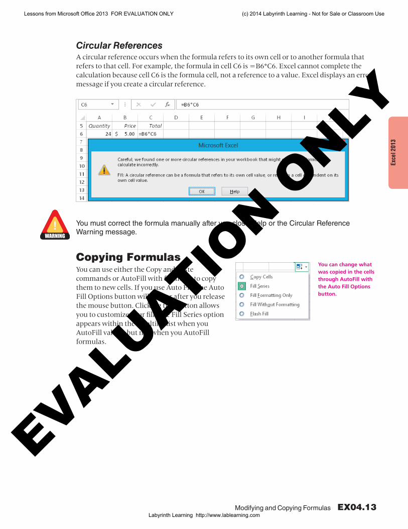
Circular ReferencesA circular reference occurs when the formula refers to its own cell or to another formula that refers to that cell. For example, the formula in cell C6 is =B6*C6. Excel cannot complete the calculation because cell C6 is the formula cell, not a reference to a value. Excel displays an error message if you create a circular reference.
WARNING
You must correct the formula manually after you close Help or the Circular Reference Warning message.
Copying FormulasYou can change what was copied in the cells through AutoFill with the Auto Fill Options button.
You can use either the Copy and Paste commands or AutoFill with formulas to copy them to new cells. If you use Auto Fill, the Auto Fill Options button will appear after you release the mouse button. Clicking this button allows you to customize your fill. The Fill Series option appears within the resulting list when you AutoFill values, but not when you AutoFill formulas.
Lessons from Microsoft Office 2013 FOR EVALUATION ONLY (c) 2014 Labyrinth Learning - Not for Sale or Classroom Use
Labyrinth Learning http://www.lablearning.com
EVALUATIO
N ONLY

EX04.14 Excel 2013 Lesson 4: Working with Formulas and Functions
DEVELOP YOUR SKILLS EX04-D04
Modify and Copy Formulas In this exercise, you will modify and copy formulas to complete your profit projection.
1. Save your file as EX04-D04-Commissions-FirstInitialLastName.
2. Select cell B8, and then follow these steps to edit the formula in the Formula Bar:
Click the D19 cell reference in the Formula Bar.
Tap [F4] to change it to an absolute reference.
Click the Enter button.
3. Double-click cell C6 to begin an in-cell edit.
4. Follow these steps to complete an in-cell edit:
Use (¢) or (¡) to position the insertion point before 5 in the formula.
Tap [Delete], type 6, and tap [Enter].
Excel displays a Circular Reference Warning message because you referred to C6, the formula cell itself.
5. Choose OK in the Circular Reference Warning message.
6. Undo the change.
Use Copy and Paste Commands to Copy a Formula
7. Select cell B14 and then use [Ctrl]+[C] to copy the formula.
8. Select cell C14 and then use [Ctrl]+[V] to paste the formula in the new cell.
This method works great if you need to copy a formula to just one cell. You can use these commands to copy a formula to a range of cells as well.
9. Select the range D14:E14 and then use [Ctrl]+[V].
The formula that you copied in step 6 is now pasted to the range of cells selected.
10. Tap [Esc] to cancel the marquee around cell B14.
Lessons from Microsoft Office 2013 FOR EVALUATION ONLY (c) 2014 Labyrinth Learning - Not for Sale or Classroom Use
Labyrinth Learning http://www.lablearning.com
EVALUATIO
N ONLY

Displaying and Printing Formulas EX04.15
Exce
l 201
3
11. Select cell D14 and look at the formula in the Formula Bar.
The relative cell reference now indicates cell D13, whereas the absolute cell reference is still looking to cell D20.
12. Follow these steps to use AutoFill to copy the formula:
Select cell C4. Drag the fill handle to cell E4.
Release the mouse button.
13. Use AutoFill to copy the formula from cell C5 to the range D5:E5.
14. Select the range B8:B15.
15. Place your mouse pointer over the fill handle at the bottom right of the selected range.
16. When you see the thin cross , drag right until the highlight includes the cells in column E and then release the mouse.
17. Deselect the filled range, and save the workbook.
Always deselect highlighted cells after performing an action to help avoid unintended changes.
Displaying and Printing FormulasVideo Library http://labyrinthelab.com/videos Video Number: EX13-V0405
Excel normally displays the results of formulas in worksheet cells, though you can choose to display the actual formulas. While formulas are displayed, Excel automatically widens columns to show more of the cell contents. Also, you can edit the formulas and print the worksheet with formulas displayed. When printing formulas, you may want to display the worksheet in Landscape orientation, due to the wider columns.
FROM THE RIBBON
Formulas→Formula Auditing→Show Formulas
FROM THE KEYBOARD[Ctrl]+[`]
Lessons from Microsoft Office 2013 FOR EVALUATION ONLY (c) 2014 Labyrinth Learning - Not for Sale or Classroom Use
Labyrinth Learning http://www.lablearning.com
EVALUATIO
N ONLY

EX04.16 Excel 2013 Lesson 4: Working with Formulas and Functions
While formulas are shown, contents will be visible for those cells in which no formulas are used.
QUICK REFERENCE VIEWING AND PRINTING FORMULAS
Task Procedure
Display or hide formulas in a workbook
■■ Choose Formulas→Formula Auditing→Show Formulas .
Change page orientation
■■ Choose Page Layout→Page Setup→Orientation→Landscape.
Print displayed formulas
■■ Choose File→Print.
■■ Choose any desired options in the Print tab and click Print.
DEVELOP YOUR SKILLS EX04-D05
Display Formulas in a WorksheetIn this exercise, you will display the formulas in the profit projection worksheet to see how it is constructed and to be able to troubleshoot any potentially inaccurate formulas.
1. Save your file as EX04-D05-Commissions-FirstInitialLastName.
2. Choose Formulas→Formula Auditing→Show Formulas .
You can use this feature to examine your formulas more closely.
3. Choose Formulas→Formula Auditing→Show Formulas again.
The values are displayed once again.
Lessons from Microsoft Office 2013 FOR EVALUATION ONLY (c) 2014 Labyrinth Learning - Not for Sale or Classroom Use
Labyrinth Learning http://www.lablearning.com
EVALUATIO
N ONLY

Using Formula AutoComplete EX04.17
Exce
l 201
3
Using Formula AutoCompleteVideo Library http://labyrinthelab.com/videos Video Number: EX13-V0406
Formula AutoComplete assists you in creating and editing formulas. Once you type an equals (=) sign and any letter(s), Excel will display a list of functions beginning with the typed letter(s) below the active cell.
Functions DefinedA function is a predefined formula that performs calculations or returns a desired result. Most functions are constructed using similar basic rules, or syntax. This syntax also applies to the Min, Max, Average, Count, and CountA functions.
Begin formulas containing functions with an equals (=) sign.
The function name follows the equals (=) sign.
A set of parentheses surrounds the argument, which is usually a range of cells.
Here, cells B6 and B8 are added to the range C10:C15.
QUICK REFERENCE USING FORMULA AUTOCOMPLETE TO ENTER A FORMULA INTO A CELL
Task Procedure
Use Formula AutoComplete
■■ Type an equals (=) sign and begin typing the formula.
■■ Double-click the formula in the list.
■■ Select the range where you will apply the formula.
■■ Type a closed parenthesis [)] to finish the formula.
DEVELOP YOUR SKILLS EX04-D06
Use Formula AutoCompleteIn this exercise, you will use the Formula AutoComplete feature to create a formula.
1. Save your file as EX04-D06-Commissions-FirstInitialLastName.
2. Click the Qtr 1 Commissions worksheet tab.
3. Select cell C11.
4. Type =ave and observe the list that results.
If you click on a function in the list, a ScreenTip will describe the function.
Lessons from Microsoft Office 2013 FOR EVALUATION ONLY (c) 2014 Labyrinth Learning - Not for Sale or Classroom Use
Labyrinth Learning http://www.lablearning.com
EVALUATIO
N ONLY
EX04.18 Excel 2013 Lesson 4: Working with Formulas and Functions
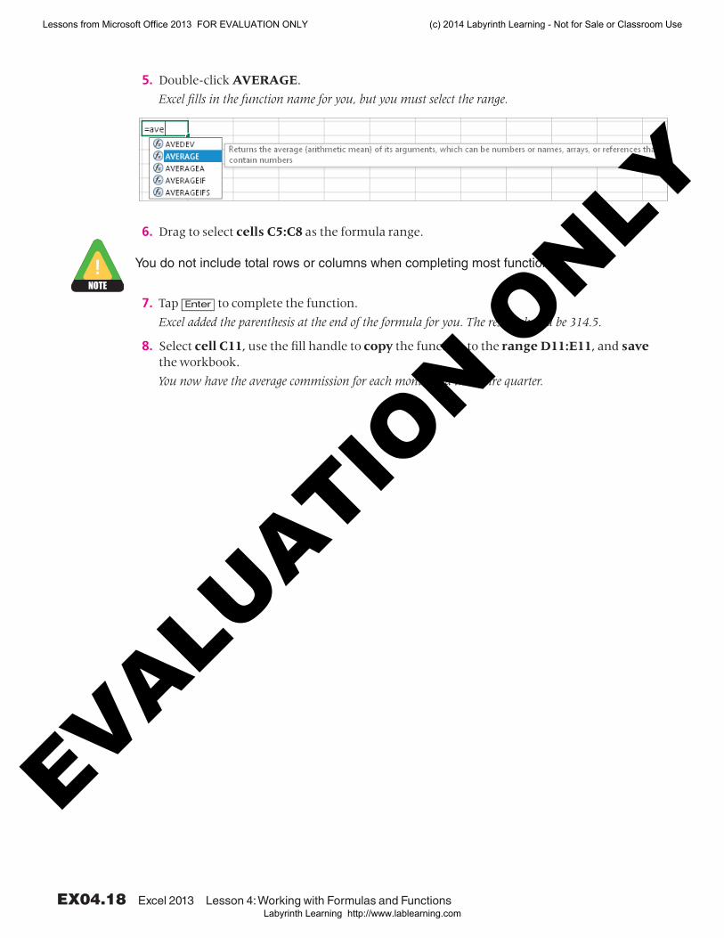
5. Double-click AVERAGE.
Excel fills in the function name for you, but you must select the range.
6. Drag to select cells C5:C8 as the formula range.
NOTE
You do not include total rows or columns when completing most functions.
7. Tap [Enter] to complete the function.
Excel added the parenthesis at the end of the formula for you. The result should be 314.5.
8. Select cell C11, use the fill handle to copy the function to the range D11:E11, and save the workbook.
You now have the average commission for each month and the entire quarter.
Lessons from Microsoft Office 2013 FOR EVALUATION ONLY (c) 2014 Labyrinth Learning - Not for Sale or Classroom Use
Labyrinth Learning http://www.lablearning.com
EVALUATIO
N ONLY

Using Insert Function EX04.19
Exce
l 201
3
Using Insert FunctionVideo Library http://labyrinthelab.com/videos Video Number: EX13-V0407
The Insert Function button displays the Insert Function dialog box. It allows you to locate a function by typing a description or searching by category. When you locate the desired function and click OK, Excel displays the Function Arguments box, which helps you enter function arguments.
The argument (typically a range) can either be typed in this box or selected from the worksheet.
You can search for a function by typing a description or choosing a category.
Excel displays the function in the Formula Bar.
The Function Arguments box appears when you choose a function.
The Collapse button hides the Function Arguments box while you select the desired range.
TIP
The Function Arguments dialog box can be moved by dragging its title bar to view the desired range on the worksheet.
QUICK REFERENCE USING INSERT FUNCTION TO ENTER A FUNCTION IN A CELL
Task Procedure
Create a function using Insert Function
■■ Select the cell in which you wish to enter a function.
■■ Click the Insert Function button.
■■ Choose the desired function; click OK.
■■ Select the ranges to include in each function argument; click OK.
Lessons from Microsoft Office 2013 FOR EVALUATION ONLY (c) 2014 Labyrinth Learning - Not for Sale or Classroom Use
Labyrinth Learning http://www.lablearning.com
EVALUATIO
N ONLY
EX04.20 Excel 2013 Lesson 4: Working with Formulas and Functions
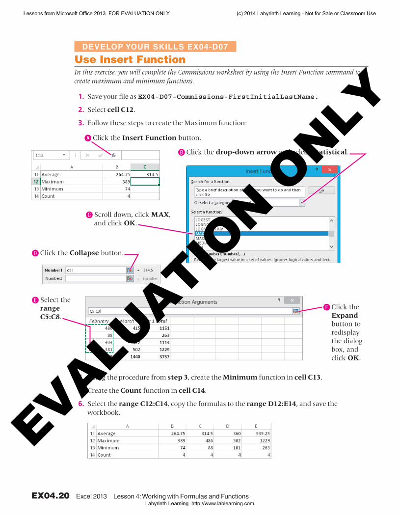
DEVELOP YOUR SKILLS EX04-D07
Use Insert FunctionIn this exercise, you will complete the Commissions worksheet by using the Insert Function command to create maximum and minimum functions.
1. Save your file as EX04-D07-Commissions-FirstInitialLastName.
2. Select cell C12.
3. Follow these steps to create the Maximum function:
Click the Insert Function button.
Click the drop-down arrow and select Statistical.
Scroll down, click MAX, and click OK.
Click the Collapse button.
Select the range C5:C8.
Click the Expand button to redisplay the dialog box, and click OK.
4. Using the procedure from step 3, create the Minimum function in cell C13.
5. Create the Count function in cell C14.
6. Select the range C12:C14, copy the formulas to the range D12:E14, and save the workbook.
Lessons from Microsoft Office 2013 FOR EVALUATION ONLY (c) 2014 Labyrinth Learning - Not for Sale or Classroom Use
Labyrinth Learning http://www.lablearning.com
EVALUATIO
N ONLY

Creating Formulas with the IF Function EX04.21
Exce
l 201
3
Creating Formulas with the IF FunctionVideo Library http://labyrinthelab.com/videos Video Number: EX13-V0408
Excel’s IF function displays a value or text based on a logical test. It displays one of two results, depending on the outcome of your logical test. For example, if you offer customers a discount for purchases of $200 or more, an IF function could be used to display either the correct discount amount or $0. For purchases greater than $200, the IF function would calculate the discount; for purchases less than $200, the formula would insert $0.
IF Function Syntax
NOTE
If you type the IF formula directly in its cell, you must add quotation (“) marks around text arguments. If you use the Insert Function command, Excel adds the quotation marks for you.
The generic parts of the IF function are shown in the following table.
Function Syntax
IF IF(logical_test, value_if_true, value_if_false)
The following table outlines the arguments of the IF function.
Argument Description
logical_test The condition being checked using a comparison operator, such as =, >, <, >=, <=, or <> (not equal to)
value_if_true The value, text in quotation (“) marks, or calculation returned if the logical test result is found to be true
value_if_false The value, text in quotation (“) marks, or calculation returned if the logical test result is found to be false
How the IF Function WorksThe formula =IF(C6>=200,C6*D6,0) is used as an example to explain the function result. Excel performs the logical test to determine whether the value in C6 is greater than or equal to 200. A value of 200 or more would evaluate as true. Any of the following would evaluate as false: a value less than 200, a blank cell, or text entered in cell C6. If the logical test proves true, the calculation C6*D6 is performed and the result displays in the formula cell. If the calculation proves false, the value 0 (zero) displays.
You may also use the IF function to display a text message or leave the cell blank. You may create complex calculations and even use other functions in arguments within an IF function, called nesting. Two examples that display text are shown in the following table.
Formula Action if True Action if False
IF(F3>150000, “Over Budget”, “Within Budget”) The text Over Budget displays The text Within Budget displays
IF(D6<=30, “”, “Late”) The cell displays blank The text Late displays
Lessons from Microsoft Office 2013 FOR EVALUATION ONLY (c) 2014 Labyrinth Learning - Not for Sale or Classroom Use
Labyrinth Learning http://www.lablearning.com
EVALUATIO
N ONLY

EX04.22 Excel 2013 Lesson 4: Working with Formulas and Functions
TIP
If you type “” (quotation marks without a space between) as the value_if_true or value_if_false argument, Excel leaves the cell blank.
DEVELOP YOUR SKILLS EX04-D08
Use the IF FunctionIn this exercise, you will use the IF function to display a text message when a salesperson achieves at least $30,000 in quarterly sales.
1. Save your file as EX04-D08-Commissions-FirstInitialLastName.
2. Type the column heading Sales in cell F4 and Met Goal? in cell G4.
3. Enter values in the range F5:F8 as shown.
4. Type Goal in cell A15 and 30000 in cell F15.
You will create a formula that compares the value in the Sales cell with the goal of $30,000. If sales are equal or greater, the message Yes displays. Otherwise, the cell displays No.
5. Select cell G5 and click the Insert Function button in the Formula Bar.
6. Follow these steps to find the IF function:
Choose Logical.
Double-click IF.
The Function Arguments dialog box appears for the IF function.
7. If necessary, move the Function Arguments dialog box out of the way by dragging its title bar until you can see column G.
8. Follow these steps to specify the IF function arguments:
Select cell F5 in the worksheet, tap [Shift]+[>], and then tap [=] (for greater than or equal to).
Select cell F15 (the $30,000 goal amount) and tap [F4].
Click in the Value_If_True box, type Yes, and tap [Tab]. (Excel adds the quotation marks.)
Enter No in the Value_If_False box. Tap [Enter].
Lessons from Microsoft Office 2013 FOR EVALUATION ONLY (c) 2014 Labyrinth Learning - Not for Sale or Classroom Use
Labyrinth Learning http://www.lablearning.com
EVALUATIO
N ONLY

Concepts Review EX04.23
Exce
l 201
3
9. Review the completed formula in the Formula Bar.
The formula is =IF(F5>=$F$15,”Yes”,”No”). The message No appears in cell G5 because Talos Bouras’ sales are not at least $30,000, the value in cell F15. The value_if_false argument applies.
10. Use AutoFill to copy the formula in cell G5 down to the range G6:G8.
The cell for Amy Wyatt displays Yes as specified by your value_if_true argument. The cells for all other salespeople display No.
Edit the IF Function
11. Select cell G5.
12. In the Formula Bar, click between the quotation (“) mark and the N, and tap [Delete] twice to delete No.
13. Click Enter in the Formula Bar.
Cell G5 does not display a message because the value_if_false argument contains no text.
14. Use AutoFill to copy the formula in cell G5 down to the range G6:G8, and save the workbook. Exit Excel.
Notice that the cells that previously displayed No in column G now display no message, as shown in the illustration below. The salespeople who met goal are easier to identify.
Concepts ReviewTo check your knowledge of the key concepts introduced in this lesson, complete the Concepts Review quiz by choosing the appropriate access option below.
If you are… Then access the quiz by…
Using the Labyrinth Video Library Going to http://labyrinthelab.com/videos
Using eLab Logging in, choosing Content, and navigating to the Concepts Review quiz for this lesson
Not using the Labyrinth Video Library or eLab Going to the student resource center for this book
Lessons from Microsoft Office 2013 FOR EVALUATION ONLY (c) 2014 Labyrinth Learning - Not for Sale or Classroom Use
Labyrinth Learning http://www.lablearning.com
EVALUATIO
N ONLY

EX04.24 Excel 2013 Lesson 4: Working with Formulas and Functions
Reinforce Your SkillsREINFORCE YOUR SKILLS EX04-R01
Create Simple FormulasIn this exercise, you will create and modify formulas using AutoSum, the keyboard, and Point Mode.
Work with Formulas and Functions
1. Start Excel. Open EX04-R01-OrdersReturns from the Excel 2013 Lesson 04 folder and save it as EX04-R01-OrdersReturns-[FirstInitialLastName].
2. Select cell E4.
3. Choose Home→Editing→AutoSum , and confirm the formula.
4. Use AutoFill to copy the formula to cells E5 and E6.
Note that the Status Bar shows the sum of the range E4:E6.
Create Formulas
5. Select cell B18.
6. Type =B4+B9+B14, and tap [Enter].
7. Use AutoFill to copy the formula to cells C18 and D18.
Use Cell References in Formulas
8. Select cell B19.
9. Type = , select cell B5, and type +.
10. Select cell B10 and type +.
11. Select cell B15 and tap [Enter].
12. Use AutoFill to copy the formula to cells C19 and D19.
The relative cell references update as you AutoFill the formula.
13. With the range B19:D19 still highlighted, AutoFill to copy the formulas to B20:D20.
Again, relative cell references allow you to AutoFill here and arrive at the correct formulas.
Lessons from Microsoft Office 2013 FOR EVALUATION ONLY (c) 2014 Labyrinth Learning - Not for Sale or Classroom Use
Labyrinth Learning http://www.lablearning.com
EVALUATIO
N ONLY

Reinforce Your Skills EX04.25
Exce
l 201
3
Modify and Copy Formulas
14. Highlight the range E4:E6.
15. Click Copy .
16. Highlight the range E9:E11.
17. Click Paste from the Ribbon.
18. Highlight the range E14:E16.
19. Click Paste.
Note that the marquee continued to surround E4:E6 after you pasted in step 17, so there was no need to click Copy prior to pasting in E14:E16.
20. Examine the formulas in the Formula Bar; then save and close the workbook. Exit Excel.
21. Submit your final file based on the guidelines provided by your instructor.To view examples of how your file or files should look at the end of this exercise, go to the student resource center.
REINFORCE YOUR SKILLS EX04-R02
Display Formulas and Use FunctionsIn this exercise, you will view formulas, use AutoComplete and Insert Function to create formulas, and use the IF Function.
Display and Print Formulas
1. Start Excel. Open EX04-R02-Contracts from the Excel 2013 Lesson 04 folder and save it as EX04-R02-Contracts-[FirstInitialLastName].
2. Tap [Ctrl]+[`] to display the worksheet formulas.
The grave accent key [`] is above the [Tab] key.
3. Choose View→Workbook Views→Page Layout View .
4. Take a few minutes to look at how the data and formulas display.
Notice that Excel widened the columns so that most of the cell contents display. In this view, the worksheet fits on two pages.
5. Choose Page Layout→Page Setup→Change Page Orientation→Landscape.
Landscape orientation prints across the wide edge of the paper, which can be useful for printing the formula view.
6. Choose Page Layout→Page Setup→Change Page Orientation→Portrait.
Portrait orientation prints across the narrow edge of the paper, which is acceptable for printing this worksheet while formulas are hidden.
7. Click the Normal View button in the Status Bar at the bottom-right corner of the window.
8. Tap [Ctrl]+[`] to hide the formulas.
Lessons from Microsoft Office 2013 FOR EVALUATION ONLY (c) 2014 Labyrinth Learning - Not for Sale or Classroom Use
Labyrinth Learning http://www.lablearning.com
EVALUATIO
N ONLY

EX04.26 Excel 2013 Lesson 4: Working with Formulas and Functions
Use Formula AutoComplete
9. Select cell A10 and edit the label to Kids for Change Contracts - Prior Year.
10. Select cell B2 and use AutoFill to copy the series Qtr 2, Qtr 3, and Qtr 4 into the range C2:E2.
11. Select cell B8.
12. Begin typing the formula =aver, and then tap [Tab] to choose AVERAGE as the function.
13. Drag to select B3:B6 and then tap [Enter].
The result should equal 33.
14. Use the fill handle to copy the formula across row 8.
The average for each quarter of the current year is now displayed.
Use Insert Function
15. Select cell B17.
16. Click Insert Function from the Formula Bar.
17. Click the drop-down arrow and select Statistical.
18. Click the Average function from the list, and click OK.
19. Modify the range to B12:B15 and confirm the formula.
The result should equal 23.5.
20. Use the fill handle to copy the formula across row 17.
21. Select cell B20.
22. Use point mode to enter the formula =B7-B16, and complete the entry.
The result should equal 38.
23. Use the fill handle to copy the formula across row 20.
The number of contracts decreased for the third quarter from 76 to 72.
Create Formulas with the IF Function
24. Select cell B21 and click Insert Function from the Formula Bar.
25. Select the IF function from the Logical category and click OK.
The Function Arguments dialog box displays.
26. For the Logical Test entry, select cell B20 in the worksheet, tap [Shift]+[>] for the greater-than symbol, and type 0.
27. Tap [Tab] to complete the entry.
28. Type Increase in the Value If True box and tap [Tab].
29. Type Decrease in the Value If False box and tap [Enter].
The result displays as Increase.
30. Use the fill handle to copy the formula across row 21; save and close the workbook. Exit Excel.
31. Submit your final files based on the guidelines provided by your instructor.To view examples of how your file or files should look at the end of this exercise, go to the student resource center.
Lessons from Microsoft Office 2013 FOR EVALUATION ONLY (c) 2014 Labyrinth Learning - Not for Sale or Classroom Use
Labyrinth Learning http://www.lablearning.com
EVALUATIO
N ONLY
Reinforce Your Skills EX04.27
Exce
l 201
3
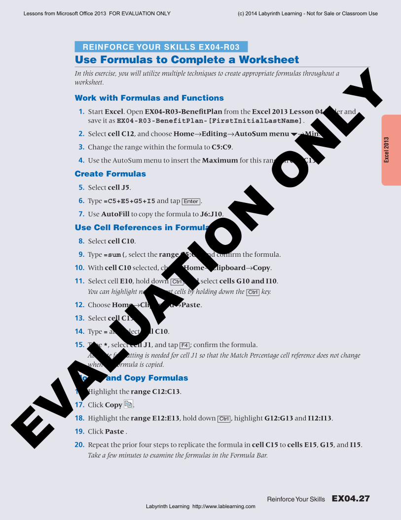
REINFORCE YOUR SKILLS EX04-R03
Use Formulas to Complete a WorksheetIn this exercise, you will utilize multiple techniques to create appropriate formulas throughout a worksheet.
Work with Formulas and Functions
1. Start Excel. Open EX04-R03-BenefitPlan from the Excel 2013 Lesson 04 folder and save it as EX04-R03-BenefitPlan-[FirstInitialLastName].
2. Select cell C12, and choose Home→Editing→AutoSum menu →Min.
3. Change the range within the formula to C5:C9.
4. Use the AutoSum menu to insert the Maximum for this range in cell C13.
Create Formulas
5. Select cell J5.
6. Type =C5+E5+G5+I5 and tap [Enter].
7. Use AutoFill to copy the formula to J6:J10.
Use Cell References in Formulas
8. Select cell C10.
9. Type =sum(, select the range C5:C9, and confirm the formula.
10. With cell C10 selected, choose Home→Clipboard→Copy.
11. Select cell E10, hold down [Ctrl], and select cells G10 and I10.
You can highlight nonadjacent cells by holding down the [Ctrl] key.
12. Choose Home→Clipboard→Paste.
13. Select cell C15.
14. Type = and select cell C10.
15. Type *, select cell J1, and tap [F4]; confirm the formula.
Absolute formatting is needed for cell J1 so that the Match Percentage cell reference does not change when the formula is copied.
Modify and Copy Formulas
16. Highlight the range C12:C13.
17. Click Copy .
18. Highlight the range E12:E13, hold down [Ctrl], highlight G12:G13 and I12:I13.
19. Click Paste .
20. Repeat the prior four steps to replicate the formula in cell C15 to cells E15, G15, and I15.
Take a few minutes to examine the formulas in the Formula Bar.
Lessons from Microsoft Office 2013 FOR EVALUATION ONLY (c) 2014 Labyrinth Learning - Not for Sale or Classroom Use
Labyrinth Learning http://www.lablearning.com
EVALUATIO
N ONLY
EX04.28 Excel 2013 Lesson 4: Working with Formulas and Functions
Display and Print Formulas
21. Choose Formulas→Formula Auditing→Show Formulas .
22. Choose View→Workbook Views→Page Layout View .
Take a few minutes to look at the way the data and formulas display.
Notice that Excel widened the columns so that most of the cell contents display.
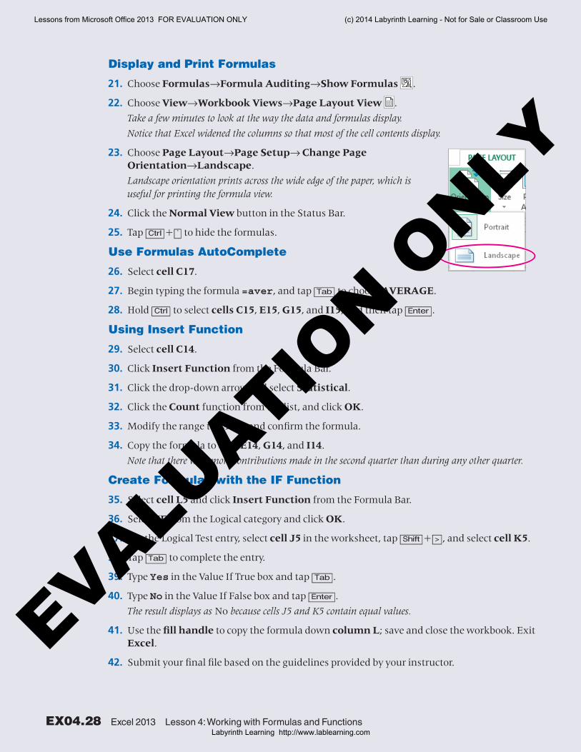
23. Choose Page Layout→Page Setup→ Change Page Orientation→Landscape.
Landscape orientation prints across the wide edge of the paper, which is useful for printing the formula view.
24. Click the Normal View button in the Status Bar.
25. Tap [Ctrl]+[`] to hide the formulas.
Use Formulas AutoComplete
26. Select cell C17.
27. Begin typing the formula =aver, and tap [Tab] to choose AVERAGE.
28. Hold [Ctrl] to select cells C15, E15, G15, and I15, and then tap [Enter].
Using Insert Function
29. Select cell C14.
30. Click Insert Function from the Formula Bar.
31. Click the drop-down arrow and select Statistical.
32. Click the Count function from the list, and click OK.
33. Modify the range to C5:C9 and confirm the formula.
34. Copy the formula to cells E14, G14, and I14.
Note that there were more contributions made in the second quarter than during any other quarter.
Create Formulas with the IF Function
35. Select cell L5 and click Insert Function from the Formula Bar.
36. Select IF from the Logical category and click OK.
37. For the Logical Test entry, select cell J5 in the worksheet, tap [Shift]+[>], and select cell K5.
38. Tap [Tab] to complete the entry.
39. Type Yes in the Value If True box and tap [Tab].
40. Type No in the Value If False box and tap [Enter].
The result displays as No because cells J5 and K5 contain equal values.
41. Use the fill handle to copy the formula down column L; save and close the workbook. Exit Excel.
42. Submit your final file based on the guidelines provided by your instructor.
Lessons from Microsoft Office 2013 FOR EVALUATION ONLY (c) 2014 Labyrinth Learning - Not for Sale or Classroom Use
Labyrinth Learning http://www.lablearning.com
EVALUATIO
N ONLY
Apply Your Skills EX04.29
Apply Your SkillsAPPLY YOUR SKILLS EX04-A01
Create Formulas, and Use Absolute ReferencesIn the exercise, you will create a price sheet with formulas that use absolute references.
Work with Formulas and Functions
1. Start Excel. Open EX04-A01-PriceChange from the Excel 2013 Lesson 04 folder and save it as EX04-A01-PriceChange-[FirstInitialLastName].
2. Use AutoSum to add the original prices in cell B13.
Create Formulas
3. Sum the discounted prices for the range C6:C11 in cell C13.
This formula will yield results when the discounted prices are entered in the worksheet.
Use Cell References in Formulas
4. Calculate the discounted price in cell C6 as Original Price * (1 – Discount Rate). Use an absolute reference when referring to the discount rate in cell B3.
5. Copy the formula in cell C6 down the column.
Cell C6 was formatted for you so it displays the price with two decimal places.
6. Change the percentage in cell B3 to 10%, and watch the worksheet recalculate.
7. Change the percentage in cell B3 back to 15%, and watch the worksheet recalculate.
You use cell references within formulas so that when changes are made, such as to the discount rate here, the formulas will recalculate properly.
Modify and Copy Formulas
8. Type Cutlery Upgrade in cell A12, and type 90 in cell B12.
Notice that the discounted price in cell C12 has automatically displayed.
9. Ensure that the discounted price in cell C12 is calculated properly; save and close the workbook. Exit Excel.
10. Submit your final file based on the guidelines provided by your instructor.To view examples of how your file or files should look at the end of this exercise, go to the student resource center.
Lessons from Microsoft Office 2013 FOR EVALUATION ONLY (c) 2014 Labyrinth Learning - Not for Sale or Classroom Use
Labyrinth Learning http://www.lablearning.com
EVALUATIO
N ONLY

EX04.30 Excel 2013 Lesson 4: Working with Formulas and Functions
APPLY YOUR SKILLS EX04-A02
Use the AVERAGE and IF FunctionsIn this exercise, you will create an IF function to indicate whether a department met the safety goal each month. You will create formulas to total the safety incidents in a six-month period, and calculate the average number of incidents per month.
Display and Print Formulas
1. Start Excel. Open EX04-A02-SafetyGoal from the Excel 2013 Lesson 04 folder and save it as EX04-A02-SafetyGoal-[FirstInitialLastName].
2. Enter January in cell A6. AutoFill down column A to display the months January through June.
3. Display the worksheet formulas.
Because you have not yet entered any formulas, nothing changes.
4. Hide the worksheet formulas.
This ensures that you will see the results of any formulas entered in upcoming steps.
Use Formula AutoComplete
5. Use AutoComplete to enter the sum function in cell B12. Add all incidents in column B within this formula.
Use Insert Function
6. Use Insert Function to enter the Average function in cell B14 to find the average number of safety incidents per month from January through June.
Your formula should return an average of one incident per month.
Create Formulas with the IF Function
7. Use the IF function to create a formula in cell C6 that indicates whether the department met its goal of no safety incidents during the month. Excel should display Met Goal if the incidents are equal to zero (0) and Not Met if the incidents are more than 0.
8. Copy the formula down the column for the months February through June; save and close the workbook. Exit Excel.
9. Submit your final file based on the guidelines provided by your instructor.To view examples of how your file or files should look at the end of this exercise, go to the student resource center.
Lessons from Microsoft Office 2013 FOR EVALUATION ONLY (c) 2014 Labyrinth Learning - Not for Sale or Classroom Use
Labyrinth Learning http://www.lablearning.com
EVALUATIO
N ONLY

Apply Your Skills EX04.31
Exce
l 201
3
APPLY YOUR SKILLS EX04-A03
Create a Financial ReportIn this exercise, you will create a worksheet by entering data, creating formulas, and using absolute references. You will also save, print a section of, and close the workbook.
Work with Formulas and Functions
1. Start Excel. Open EX04-A03-NetProfit from the Excel 2013 Lesson 04 folder and save it as EX04-A03-NetProfit-[FirstInitialLastName].
2. Use AutoSum to add the revenue in cell F4.
Create Formulas
3. Type a formula in cell B10 to sum the costs for Q1 in column B.
Practice typing the cell references here. You will use Point Mode later.
4. AutoFill the quarter headings in row 3 and the Total Costs formula in row 10.
Ensure that you AutoFill the total costs through column F.
Use Cell References in Formulas
5. Use a formula to calculate employee costs in cell B6. The formula should multiply the revenue (cell B4) by the percentage (cell B15). Use a mixed reference to refer to the revenue and an absolute reference to refer to the cost percentage.
6. Copy the titles in the range A6:A9 to the range A15:A18.
7. Use formulas to calculate the other costs in the range B7:B9. Each formula should multiply the revenue in row 4 by the related cost percentage in rows 16–18.
8. Calculate the net profit in cell B13 as Gross Profit * (1 – Tax Rate). Once again, use an absolute reference when referring to the tax rate in cell B19.
Your Net Profit should equal 169,740.
Modify and Copy Formulas
9. Modify the formula in cell B12 to calculate Gross Profit as Revenue minus Total Costs.
10. Copy the range B12:B13 to the range C12:F13.
11. Copy the formulas in the range B6:B9 to the range C6:E9.
Display and Print Formulas
12. Display the worksheet formulas.
Review the formulas to ensure that they have been entered correctly.
13. Hide the worksheet formulas.
Lessons from Microsoft Office 2013 FOR EVALUATION ONLY (c) 2014 Labyrinth Learning - Not for Sale or Classroom Use
Labyrinth Learning http://www.lablearning.com
EVALUATIO
N ONLY
EX04.32 Excel 2013 Lesson 4: Working with Formulas and Functions
Use Formula AutoComplete
14. Use AutoComplete to calculate Total Employee Costs in cell F6.
15. Copy the formula from cell F6 to cell F7.
The Total Capital Expenditures in cell F7 should equal 377,300.
Use Insert Function
16. Use the Insert Function Dialog Box to sum the Total Materials Costs in cell F8.
17. Copy the formula from cell F8 to cell F9.
Create Formulas with the IF Function
18. Create an IF Function in cell H12 to determine if the Annual Gross Profit Goal in cell H4 has been met. Excel should display Met Goal if it has been met and Missed Goal if it has not been met. Save and close the workbook. Exit Excel.
Since the Gross Profit of 463,050 is less than the 500,000 goal in cell H4, Missed Goal is displayed in cell H12.
19. Submit your final file based on the guidelines provided by your instructor.
Lessons from Microsoft Office 2013 FOR EVALUATION ONLY (c) 2014 Labyrinth Learning - Not for Sale or Classroom Use
Labyrinth Learning http://www.lablearning.com
EVALUATIO
N ONLY

Extend Your Skills EX04.33
Extend Your SkillsIn the course of working through the Extend Your Skills exercises, you will think critically as you use the skills taught in the lesson to complete the assigned projects. To evaluate your mastery and completion of the exercises, your instructor may use a rubric, with which more points are allotted according to performance characteristics. (The more you do, the more you earn!) Ask your instructor how your work will be evaluated.
EX04-E01 That’s the Way I See ItYou are known as the neighborhood Excel expert for small businesses! The chamber of commerce has asked you to create a worksheet analyzing three different retail businesses in your area so they can determine the profitability of the businesses in order to help develop marketing plans for the individual chamber members as well as the community at large. You will evaluate the local competition for each business, and create a formula that shows how well positioned the three companies are in the marketplace.
Open EX04-E01-Competition from the Excel 2013 Lesson 04 folder and save it as EX04-E01-Competition-[FirstInitialLastName].
Enter three companies and their industries at the top of the worksheet. Be sure to select companies from three different industries (electronics, women’s clothing, etc.). Enter the direct competitors for each company within the spreadsheet, and create formulas that will display the number of competitors for each. Lastly, include a formula that designates companies with three or more competitors as having “High” competition, and companies with fewer than three competitors as having “Low” competition.
You will be evaluated based on the inclusion of all elements specified, your ability to follow directions, your ability to apply newly learned skills to a real-world situation, your creativity, and the relevance of your topic and/or data choice(s). Submit your final file based on the guidelines provided by your instructor.
EX04-E02 Be Your Own BossIn this exercise, you will create a customer listing that shows the number of jobs performed for each customer of Blue Jean Landscaping, and the billings associated with each.
Open EX04-E02-CustomerBase from the Excel 2013 Lesson 04 folder and save it as EX04-E02-CustomerBase-[FirstInitialLastName].
Create formulas in the designated cells within column B to determine the total number of jobs for each company type and to count the number of companies of each type. For the Billings Increase columns, first place the increase percentages in a suitable location within the spreadsheet, and then use absolute formatting to create formulas for each company referencing these percentages. Format the worksheet using your knowledge of Excel, ensuring that all numbers are displayed properly. Since this is your company, write a paragraph with at least five sentences that summarizes the data you have calculated. Type the paragraph below the data. In it, explain what you have learned from the calculations and how you might change how you do business as a result.
You will be evaluated based on the inclusion of all elements specified, your ability to follow directions, your ability to apply newly learned skills to a real-world situation, your creativity, and your demonstration of an entrepreneurial spirit. Submit your final file based on the guidelines provided by your instructor.
Lessons from Microsoft Office 2013 FOR EVALUATION ONLY (c) 2014 Labyrinth Learning - Not for Sale or Classroom Use
Labyrinth Learning http://www.lablearning.com
EVALUATIO
N ONLY

EX04.34 Excel 2013 Lesson 4: Working with Formulas and Functions
Transfer Your SkillsIn the course of working through the Transfer Your Skills exercises, you will use critical-thinking and creativity skills to complete the assigned projects using skills taught in the lesson. To evaluate your mastery and completion of the exercises, your instructor may use a rubric, with which more points are allotted according to performance characteristics. (The more you do, the more you earn!) Ask your instructor how your work will be evaluated.
EX04-T01 Use the Web as a Learning ToolThroughout this book, you will be provided with an opportunity to use the Internet as a learning tool by completing WebQuests. According to the original creators of WebQuests, as described on their website (WebQuest.org), a WebQuest is “an inquiry-oriented activity in which most or all of the information used by learners is drawn from the web.” To complete the WebQuest projects in this book, navigate to the student resource center and choose the WebQuest for the lesson on which you are currently working. The subject of each WebQuest will be relevant to the material found in the lesson.
WebQuest Subject: Utilizing the IF function when classifying restaurant chains as successful or unsuccessful
Submit your final file(s) based on the guidelines provided by your instructor.
EX04-T02 Demonstrate ProficiencyYou have decided to recreate the Product Markup Worksheet for Stormy BBQ to make it more user-friendly. Specifically, you would like to remove the markup percentages from individual formulas. You want to replace them with a cell reference from the worksheet that contains the markup percentage.
Open EX04-T02-ProductMarkup from the Excel 2013 Lesson 04 folder and save it as EX04-T02-ProductMarkup-[FirstInitialLastName]. Use the formula writing and absolute formatting skills that you have learned in this lesson to create the markup formulas described above and produce a more user-friendly worksheet. Format the worksheet as desired, ensuring that all numbers are properly formatted and will appear in a logical manner when printed.
Submit your final file based on the guidelines provided by your instructor.
Lessons from Microsoft Office 2013 FOR EVALUATION ONLY (c) 2014 Labyrinth Learning - Not for Sale or Classroom Use
Labyrinth Learning http://www.lablearning.com
EVALUATIO
N ONLY