(4th supplementary slides: computer vision) · (4th supplementary slides: computer vision) ......

(4th Supplementary Slides: Computer Vision)

Professor John Daugman

University of Cambridge

Computer Science Tripos, Part IILent Term 2015/16

1 / 33

Face Detection, Recognition, and Interpretation

Some variations in facial appearance (L.L. Boilly: Reunion de Tetes Diverses)2 / 33

(Face Detection, Recognition, and Interpretation, con’t)

Detecting faces and recognising their identity is a “Holy Grail” problemin computer vision. It is difficult for all the usual reasons:

I Faces are surfaces on 3D objects (heads), so facial images dependon pose and perspective angles, distance, and illumination

I Facial surfaces have relief, so some parts (e.g. noses) can occludeother parts. Hair can also create random occlusions and shadows

I Surface shape causes shading and shadows to depend upon the angleof the illuminant, and whether it is an extended or a point source

I Faces have variable specularity (dry skin may be Lambertian,whereas oily or sweaty skin may be specular). As always, thisconfounds the interpretation of the reflectance map

I Parts of faces can move around relative to other parts (eye or lipmovements; eyebrows and winks). We have 7 pairs of facial muscles.People use their faces as communicative organs of expression

I People put things on their faces (e.g. glasses, cosmetics, cigarettes),change their facial hair (moustaches, eyebrows), and age over time

3 / 33


Classic problem: within-class variation (same person, different conditions)can exceed the between-class variation (different persons).

These are different persons, in genetically identical (monozygotic) pairs:

4 / 33



Persons who share 50% of their genes (parents and children; full siblings;double cousins) sometimes look almost identical (apart from age cues):

5 / 33



...and these are completely unrelated people, in Doppelganger pairs:Photos by François Brunelle of unrelated doppelgängers

6 / 33



Same person, fixed pose and expression; varying illumination geometry:

BELHUMEUR ET AL.: EIGENFACES VS. FISHERFACES: RECOGNITION USING CLASS SPECIFIC LINEAR PROJECTION 715

3 EXPERIMENTAL RESULTS

In this section, we present and discuss each of the afore-mentioned face recognition techniques using two differentdatabases. Because of the specific hypotheses that wewanted to test about the relative performance of the consid-ered algorithms, many of the standard databases were in-appropriate. So, we have used a database from the HarvardRobotics Laboratory in which lighting has been systemati-cally varied. Secondly, we have constructed a database atYale that includes variation in both facial expression andlighting. 1

3.1 Variation in LightingThe first experiment was designed to test the hypothesisthat under variable illumination, face recognition algo-rithms will perform better if they exploit the fact that im-ages of a Lambertian surface lie in a linear subspace. Morespecifically, the recognition error rates for all four algo-rithms described in Section 2 are compared using an im-age database constructed by Hallinan at the Harvard Ro-botics Laboratory [14], [15]. In each image in this data-base, a subject held his/her head steady while being illu-minated by a dominant light source. The space of lightsource directions, which can be parameterized by spheri-cal angles, was then sampled in 15$ increments. See Fig. 3.From this database, we used 330 images of five people (66of each). We extracted five subsets to quantify the effectsof varying lighting. Sample images from each subset areshown in Fig. 4.

Subset 1 contains 30 images for which both the longitudi-nal and latitudinal angles of light source direction arewithin 15$ of the camera axis, including the lighting

1. The Yale database is available for download from http://cvc.yale.edu.

direction coincident with the camera’s optical axis.Subset 2 contains 45 images for which the greater of the

longitudinal and latitudinal angles of light source di-rection are 30$ from the camera axis.

Subset 3 contains 65 images for which the greater of thelongitudinal and latitudinal angles of light source di-rection are 45$ from the camera axis.



For all experiments, classification was performed using anearest neighbor classifier. All training images of an indi-

Fig. 3. The highlighted lines of longitude and latitude indicate the lightsource directions for Subsets 1 through 5. Each intersection of a lon-gitudinal and latitudinal line on the right side of the illustration has acorresponding image in the database.

Fig. 4. Example images from each subset of the Harvard Database used to test the four algorithms.

7 / 33



Effect of variations in pose angle (easy and hard), and distance:

8 / 33



Changes in appearance over time (sometimes artificial and deliberate)

9 / 33

Paradox of Facial Phenotype and Genotype

Facial appearance (phenotype) of everyone changes over time with age;but monozygotic twins (identical genotype) track each other as they age.

Therefore at any given point in time, they look more like each other thanthey look like themselves at either earlier or later periods in time

10 / 33


Detecting and recognising faces raises all the usual questions encounteredin other domains of computer vision:

I What is the best representation to use for faces?

I Should this be treated as a 3D problem (object-based, volumetric),or a 2D problem (image appearance-based)?

I How can invariances to size (hence distance), location, pose, andillumination be achieved? (A given face should acquire a similarrepresentation under such transformations, for matching purposes.)

I What are the generic (i.e. universal) properties of all faces that wecan rely upon, in order to reliably detect the presence of a face?

I What are the particular features that we can rely upon to distinguishamong faces, and thus determine the identity of a given face?

I What is the best way to handle “integration of evidence”, andincomplete information, and to make decisions under uncertainty?

I How can machine learning develop domain expertise, either aboutfaces in general (e.g. pose transformations), or facial distinctions?

11 / 33

Viola-Jones Face Detection Algorithm

Paradoxically, face detection is a harder problem than recognition, andperformance rates of algorithms are poorer. (It seems paradoxical sincedetection precedes recognition; but recognition performance is measuredonly with images already containing faces.) The best known way to findfaces is the cascade of classifiers developed by Viola and Jones (2004).

shift the detector window by more than one pixel at a time depending on thecurrent window size, and the scale would be increased by some constant (say20%) at each iteration over the image, but the number of evaluations will stillbe about 105 per image.

Modern approaches to face detection make use of a number of image pro-cessing and machine learning techniques to deal with these challenges. Thecurrently most popular method is due to Viola and Jones (2004), who popu-larised the use of the AdaBoost (“Adaptive Boosting,” formulated by Freundand Schapire) machine learning algorithm to train a cascade of feature clas-sifiers for object detection and recognition. Boosting is a supervised machinelearning framework which works by building a “strong classifier” as a com-bination of (potentially very simple) “weak classifiers.” As illustrated in thefigure below, a Viola-Jones face detector consists of classifiers based on simplerectangular features (which can be viewed as approximating Haar wavelets)and makes use of an image representation known as the integral image (alsocalled summed area table) to compute such features very efficiently.

The resulting boosted classifier is a weighted combination of thresholdedresponses to a set of rectangular features that, like Haar basis functions, differin complexity (e.g. the features may consist of 2, 3 or 4 rectangular regions),scale, position, and orientation (horizontal or vertical, though some implemen-tations also incorporate diagonal features). Formally, a weak classifier hj(x)

97

12 / 33

(Viola-Jones Face Detection Algorithm, con’t)

Key idea: build a strong classifier from a cascade of many weak classifiers− all of whom in succession must agree on the presence of a face

I A face (in frontal view) is presumed to have structures that shouldtrigger various local “on-off” or “on-off-on” feature detectors

I A good choice for such feature detectors are 2D Haar wavelets(simple rectangular binary alternating patterns)

I There may be 2, 3, or 4 rectangular regions (each +1 or −1) formingfeature detectors fj , at differing scales, positions, and orientations

I Applying Haar wavelets to a local image region only involves addingand subtracting pixel values (no multiplications; hence very fast)

I A given weak classifier hj (x) consists of a feature fj , a threshold θj

and a polarity pj ∈ ±1 (all determined in training) such that

hj (x) =

{−pj if fj < θj

pj otherwise

I A strong classifier h(x) takes a linear combination of weak classifiers,using weights αj learned in a training phase, and considers its sign:

h(x) = sign(∑

j

αj hj )

13 / 33

(Viola-Jones Face Detection Algorithm, con’t)I At a given level of the cascade, a face is “provisionally deemed to

have been detected” at a certain position if h(x) > 0I Only those image regions accepted by a given layer of the cascade

(h(x) > 0) are passed on to the next layer for further considerationI A face detection cascade may have 30+ layers, yet the vast majority

of candidate image regions will be rejected early in the cascade.

shift the detector window by more than one pixel at a time depending on thecurrent window size, and the scale would be increased by some constant (say20%) at each iteration over the image, but the number of evaluations will stillbe about 105 per image.

Modern approaches to face detection make use of a number of image pro-cessing and machine learning techniques to deal with these challenges. Thecurrently most popular method is due to Viola and Jones (2004), who popu-larised the use of the AdaBoost (“Adaptive Boosting,” formulated by Freundand Schapire) machine learning algorithm to train a cascade of feature clas-sifiers for object detection and recognition. Boosting is a supervised machinelearning framework which works by building a “strong classifier” as a com-bination of (potentially very simple) “weak classifiers.” As illustrated in thefigure below, a Viola-Jones face detector consists of classifiers based on simplerectangular features (which can be viewed as approximating Haar wavelets)and makes use of an image representation known as the integral image (alsocalled summed area table) to compute such features very efficiently.

The resulting boosted classifier is a weighted combination of thresholdedresponses to a set of rectangular features that, like Haar basis functions, differin complexity (e.g. the features may consist of 2, 3 or 4 rectangular regions),scale, position, and orientation (horizontal or vertical, though some implemen-tations also incorporate diagonal features). Formally, a weak classifier hj(x)

97

14 / 33

(Viola-Jones Face Detection Algorithm, con’t)I Training uses the AdaBoost (“Adaptive Boosting”) algorithmI This supervised machine learning process adapts the weights αj such

that early cascade layers have very high true accept rates, say 99.8%(as all must detect a face; hence high false positive rates, say 68%)

I Later stages in the cascade, increasingly complex, are trained to bemore discriminating and therefore have lower false positive rates

I More and more 2D Haar wavelet feature detectors are added to eachlayer and trained, until performance targets are met

I The cascade is evaluated at different scales and offsets across animage using a sliding window approach, to find any (frontal) faces

I With “true detection” probability di in the i th layer of an N-layercascade, the overall correct detection rate is: D =

∏Ni=1 di

I With “erroneous detection” probability ei at the i th layer, the overallfalse positive rate is E =

∏Ni=1 ei (as every layer must falsely detect)

I Example: if we want no false detections, with 105 image subregionsso E < 10−5, in a 30-layer cascade we train for ei = 10−5/30 ≈ 0.68which shows why each layer can use such weak classifiers!

I Likewise, to achieve a decent overall detection rate of D = 0.95requires di = 0.951/30 ≈ .9983 (very happy to call things “faces”)

15 / 33

(Viola-Jones Face Detection Algorithm, con’t)

Performance on a local group photograph:

consists of a feature fj, a threshold θj and a parity pj ∈ ±1 such that

hj(x) =

1 if pjfj < pjθj−1 otherwise

and the resulting strong classifier using weights aj is

h(x) = sign(∑

j

ajhj)

By combining such classifiers into a hierarchical cascade made up of increas-ingly complex classifiers, good detection accuracy can be achieved at relativelylow false positive levels. The cascade is also very efficient, since each stage(layer) is computationally very simple to apply to an image region and onlythose regions which are accepted by a given layer of the cascade (h(x) > 0)are passed on to the next layer for consideration. Training is done in sucha way that early cascade layers have very high true accept rates (with cor-respondingly high false positive rates) in order to quickly reject those imageregions that are very unlikely to represent a face. Later stages are trained tobe more discriminating and consequently have increasingly lower target falsepositive rates. Each stage is trained by adding rectangle features until thetarget detection and false positive rates are met.

A fully trained face detection cascade may have over 30 layers, yet the vastmajority of candidate image regions will only be considered by the first few ofthese. To perform face detection, the cascade is evaluated at different scalesand offsets within an image using a sliding window approach. The followingfigure illustrates what the sliding window finds in a local group photo:

9816 / 33

2D Appearance-based Face Recognition: Gabor Wavelets

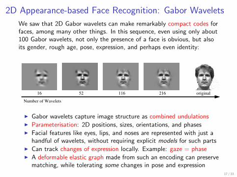
We saw that 2D Gabor wavelets can make remarkably compact codes forfaces, among many other things. In this sequence, even using only about100 Gabor wavelets, not only the presence of a face is obvious, but alsoits gender, rough age, pose, expression, and perhaps even identity:

Number of Wavelets

116 216 original16 52

�� !�!"$#%��&'��(%��&)�!*,+-��&/.0*1� 23�� 4#5&6#5(7�,8!��":9;+��$<$��=��4&'�>@?BA CED:F�GIHKJMLON-PBHRQ3PBN�J7DBS�TUS�VXWYGID:Z�[6J�\]@^�`_a��b�c^�d!e6fhg�i1jlk�monEpqkc� or7��ts4d ubvX��uwk$d xr�di�d^�;u�i7s�kcuKy%uzd��@�te {5i�|%eBxe�icj�d^��m;k1}Kic�6y%uzd��!ea~l��m;k1}Kic�@_@k��c�ub4dj/��|%s�d��i�|%e�k1�X|�i1d,ic� d ^%ic�ci�|%k1u��Id ^��%e��,{�ubv��|��d ^%k1dt�-j/i��k��c�b�ct|�j�k1�,��ubv��i1jom;kc}5i��_@k��ctu��det��d��we�|�i1d,{5i�e e �b}�u��d is�k1uws4�%ubk1d �k�_a��b�c^�d`fhg@}�v0k�e ��,{�ub,{��i1�:ts4d �bic|0icj�d ^%�m;kc}5i��`_@k��ctu��d`~-�c�3ic|�d i�d ^�,�b��k1�c��|0j�k�s�dt��k�j�k1�,�bu�v�i1j6r7�5k1u_ak��ub4de��@�~ ��t� �~ ��h ^5kce�d i�}K0s4ic|5eB�wr7��tr��¡]@^�¢_@k��c�ub4d£�~ �1¤ �be�d^�¥r7�%k1uh_@k��ctu��d�icj3d^�¢_ak��ub4d,~ � ��¦§ ~ � �!¨ �~ �c¤�© ��ª g�« ¬ �¥n�zd^��®�°¯ �~ �� ¨ ��t� ¨ �~ ��6±:² �l_6�stk1|³_h��zdµ´ § ��¨K�� ©�¶ �·� �,�¥��|³i1d^��_6i��r%e��I�c�b�c�|�¸�¹�ºR»¼¯'½�» ±k1|%r³k�monEp®�®�¾�t~ �� ¨ �� ¨B~ ��h ��d ^��ic{7d��kcu�_a��b�c^�de�j/ic��¸Od ^%k1d��,�b|��,�b¿��d ^��|�t� ��v��b|ÀtÁK�À¯'Â ± kc� ��|³}�vf g � § ¸¼¨ �~ � � © ��)dÃs�kc|¢}5�e ^�i$_h|�d ^%k1d �~ � �-�ÅÄ ¬3Æ ��ÇRÈ�É g�« ¬ ~ �c¤ ��_h^%�� g�« ¬ � § ~ � �!¨B~ �1¤�© �

ÊÌËYÍÎ ÏÎ

ÐËË Ñ

ÒoÓ�Ô�Õ�Ó%Ö

Õ�×

�� Â7 �ØÅ9!(7#K��&'��"1#¥¸O¹Ùº�»K¯�½l» ± �w��ÚcÚ%�!*�8�Û¢&�.%�,=Ü��#K�!�1��Ú�ÚK��#��Ý��#5&)"¡&/.��Ù<$��&�"$�ßÞà¹á½lâ¥ãåä¼.��³��Ú�ÚK��#��E":9ßÞæ��#5&)"�º�»K¯�½l» ± �w��c�!.��<��!*�+-��&�.³&�.%�X=z��#K�!�$��Ú�ÚK��#��¢�,ã�ç`"$&/.��Ú�ÚK��#��$��!"$#%��&'��&�(7&)��$#"$��&/.�"��"1#K�1=lÚK� ":è��!�4&��"$#q":90��9!(7#¼�4&��"$#³¸é¹éº�»5¯'½�» ± ��#5&)"�&/.��¥��(%8��Ú%�c�!�ê �£ë�ìÀº�»K¯�½l» ± ã

]@^%�k1}Ki$�cotÁ��%k$d��i�|%ehk1ububi$_E�%e@di,r�4y%|�;d^��ic{K��!k$dic�í7î $º » ¯�½ » ±�ï ðKñ ê ¯/~ �� ¨ �t�� ¨ ~ ��± ë ¯'ò ±

kce6j/icubu�i$_Ãet l�c�b�ct|ßk,e 4d`�óicjIi�{7d �b��k1uR_@k��c�ub4d!eai1j-k,monEp��7d ^%�ic{K��!k$d i�� í î ��{��te �|�d!eakc|�i��Bd^�ic��ic|%kcu5{%� ic�:ts�d��i�|�icj�kj/��|%s�d��i�|ß¸Xic|�d i�d ^%�s4ubi�e tr�u��b|�tkc�heB{%kc|¢i1j-�U¯�e ��xÁ5�Ã¯'ò ± k1|5r�y5�%��Â ± ��'� c�

ô¸�� í î ¯�¸ ± �å¸@��;�õ� âö g�÷ È fhg'~l��¥��_h��d ^éÞø�¸h�� ¯�ù ±ú û¢ü�ýhþåÿ��-ü�ý�� ü� �þ��þ��¢ü�ýhþ]@^��_@k��ctu��d��{��te �|�dk1d �bic|r7xe s�� b}5xrE�b|Ed^�O{%� t��bic�5e�e ts�d��i�|µ��k�vM}5Ù4¦¼ts4d �b�ctu�vM�%e trEj/ic�¢k��|�Oj�kcs4�d �!kcs��b|��%� ak�eB�ws�kcu�ubvc��d^��behdkce!��wehkcs!^%��t�ctr�}�v�k"�,|%�ubv�r74j/i�� ,�b|��kXmonEp£e i�d^%k$dÃ��dÃ��k$d!s!^�te@d^�;j�kcs�;��k1��|¢xkcs!^�j/�kc��;icjlk��wr7tiÃeBxÁ��%�|%s�c�I]@^%�k��|�ar74j/i�� k$d��i�|;i1j%k3monEp��beIs�k1��xr`i��7d�}�v�s4i�|%eB�wr7t� �b|��@d ^%��|�d �b��_ak��ub4d�|��d:_6i��!�okceIkÃeB�b|��u�

I Gabor wavelets capture image structure as combined undulationsI Parameterisation: 2D positions, sizes, orientations, and phasesI Facial features like eyes, lips, and noses are represented with just a

handful of wavelets, without requiring explicit models for such partsI Can track changes of expression locally. Example: gaze = phaseI A deformable elastic graph made from such an encoding can preserve

matching, while tolerating some changes in pose and expression17 / 33

(2D Appearance-based Face Recognition: Gabor Wavelets)

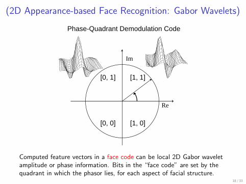
Phase-Quadrant Demodulation Code

[0, 0] [1, 0]

[1, 1][0, 1]

Re

Im

Computed feature vectors in a face code can be local 2D Gabor waveletamplitude or phase information. Bits in the “face code” are set by thequadrant in which the phasor lies, for each aspect of facial structure.

18 / 33

2D Appearance-based Face Recognition: “Eigenfaces”

An elegant method for 2D appearance-based face recognition combinesPrincipal Components Analysis (PCA) with machine learning and algebra,to compute a linear basis (like the Fourier basis) for representing any faceas a combination of empirical eigenfunctions, called eigenfaces.

I A database of face images (at least 10,000) that are pre-normalisedfor size, position, and frontal pose is “decomposed” into its PrincipalComponents of statistical variation, as a sequence of orthonormaleigenfunctions whose eigenvalues are in descending order

I This is a classical framework of linear algebra, associated also withthe names Karhunen-Loeve Transform, or the Hotelling Transform,or Dimensionality Reduction and subspace projection

I Optimised for truncation: finding the best possible (most accurate)representation of data using any specified finite number of terms

I Having extracted from a face gallery the (say) 20 most importanteigenfaces of variation (in sequence of descending significance),any given presenting face is projected onto these, by inner product

I The resulting (say) 20 coefficients then constitute a very compactcode for representing, and recognising, the presenting face

I 15 such representational eigenfaces are shown in the next slide19 / 33

(2D Appearance-based Face Recognition: “Eigenfaces”)

The top left face is a particular linear combination of the eigenfaces20 / 33

(2D Appearance-based Face Recognition: “Eigenfaces”)

I Performance is often in the range of 90% to 95% accuracy

I Databases can be searched very rapidly, as each face is representedby a very compact feature vector of only about 20 numbers

I A major limitation is that significant (early, low-order) eigenfacesemerging from the statistical analysis arise just from normalisationerrors of size (head outlines), or variations in illumination angle

I Like other 2D representations for faces, the desired invariances fortransformations of size (distance), illumination, and pose are lacking

I Both the Viola-Jones face detection algorithm, and these 2Dappearance-based face recognition algorithms, sometimes deploy“brute force” solutions (say at airport Passport control) such asacquiring images from a large (3× 3) or (4× 4) array of cameras fordifferent pose angles, each allowing some range of angles

21 / 33

Three-Dimensional Approaches to Face Recognition

Face recognition algorithms now aim to model faces as three-dimensionalobjects, even as dynamic objects, in order to achieve invariances for pose,size (distance), and illumination geometry. Performing face recognition inobject-based (volumetric) terms, rather than appearance-based terms,unites vision with model-building and graphics.

To construct a 3D representation of a face, it is necessary to extract botha shape model (below right), and a texture model (below left). The term“texture” here encompasses albedo, colouration, and 2D surface details.

16.6 Three-dimensional approaches to face recognition

Current efforts in face recognition seek to model faces as three-dimensionalobjects, even as dynamic objects, in order to achieve invariance both to poseangle and illumination geometry. Of course, this requires solving the ill-posedproblems of infering shape from shading, interpreting albedo versus variationsin Lambertian and specular surface properties, structure from motion, etc.On page 4 we examined how difficult this problem is, and how remarkable itis that we humans seem to be so competent at it. The synthesis of visionas model-building and graphics, to perform face recognition in object-basedterms, rather than appearance-based terms, is now a major focus of this field.

In order to construct a 3D representation of a face (so that, for example,its appearance can be predicted at different pose angles as we saw on page 4),it is necessary to extract separately both a shape model and a texture model(texture encompasses albedo, colouration, any 2D surface details, etc).

The 3D shape model (above right) is extracted by various means, whichmay include laser range-finding (with millimetre resolution); stereo cameras;projection of structured light (grid patterns whose distortions reveal shape); orextrapolation from a multitude of images taken from different angles (often a4×4 matrix). The size of the data structure can be in the gigabyte range, andsignificant time is required for the computation. Since the texture model islinked to coordinates on the shape model, it is possible to project the texture(tone, colour, features, etc) onto the shape and thereby generate models ofthe face in different poses. Clearly sensors play an important role here forextracting the shape model, but it is also possible to do this even from a singlephotograph if sufficiently strong Bayesian priors are also marshalled, assumingan illumination geometry and universal aspects of head and face shape.

103

22 / 33

(Three-Dimensional Approaches to Face Recognition)

Extracting the 3D shape model can be done by various means:

I laser range-finding, even down to millimetre resolution

I calibrated stereo cameras

I projection of structured IR light (grid patterns whose distortionsreveal shape, as with Kinect)

I extrapolation from multiple images taken from different angles

The size of the resulting 3D data structure can be in the gigabyte range,and significant time can be required for the computation.

Since the texture model is linked to coordinates on the shape model, it ispossible to “project” the texture (tone, colour, features) onto the shape,and thereby to generate predictive models of the face in different poses.

Clearly sensors play an important role here for extracting shape models,but it is also possible to do this even from just a single photograph ifsufficiently strong Bayesian priors are also marshalled, assuming anillumination geometry and some universal aspects of head and face shape.

23 / 33


Texture Extraction& Facial Expression

Reconstructionof Shape & Texture Cast Shadow New Illumination Rotation

InitializationOriginal 3D Reconstruction

An impressive demo of using a single 2D photograph (top left) to morpha 3D face model after manual initialisation, building a 3D representationof the face that can be manipulated for differing pose angles, illuminationgeometries, and even expressions, can be seen here:

http://www.youtube.com/watch?v=nice6NYb_WA

24 / 33

http://www.youtube.com/watch?v=nice6NYb_WA


Description from the Blanz and Vetter paper,Face Recognition Based on Fitting a 3D Morphable Model:

“...a method for face recognition across variations in pose, ranging fromfrontal to profile views, and across a wide range of illuminations,including cast shadows and specular reflections. To account for thesevariations, the algorithm simulates the process of image formation in 3Dspace, using computer graphics, and it estimates 3D shape and texture offaces from single images. The estimate is achieved by fitting a statistical,morphable model of 3D faces to images. The model is learned from a setof textured 3D scans of heads. Faces are represented by modelparameters for 3D shape and texture.”

25 / 33

Face Algorithms Compared with Human Performance

The US National Institute for Standards and Technology (NIST) runsperiodic competitions for face recognition algorithms, over a wide rangeof conditions. Uncontrolled illumination and pose remain challenging.But in a 2007 test, three algorithms had ROC curves above (better than)human performance at non-familiar face recognition (the black curve):

Performance of humans and seven algorithms on the difficult face pairs (Fig. 3a) and easy face pairs (Fig. 3b) shown

algorithms outperform humans on the difficult face pairs at most or all combinations of verification

(cf., [20] NJIT, [21] CMU for details on two of the three algorithms). Humans out-perform the other four

face pairs. All but one algorithm performs more accurately than humans on the easy face pairs. (A color

figure is provided in the Supplemental Material.)

0

0.2

0.4

0.6

0.8

1

0 0.1 0.2 0.3 0.4 0.5 0.6 0.7 0.8 0.9 1

False Accept Rate

Verif

icati

on

Rate

NJIT

CMU

Viisage

Human Performance

Algorithm A

Algorithm B

Algorithm C

Algorithm D

Chance Performance

26 / 33

Major Breakthrough in 2015: Deep-Learning “FaceNet”

Machine learning approaches focused on scale (“Big Data”) are having aprofound impact in Computer Vision. In 2015 Google demonstrated largereductions in face recognition error rates (by 30%) on two very difficultdatabases: YouTube Faces (95%), and Labeled Faces in the Wild (LFW)database (99.63%), which are new accuracy records.

27 / 33

(Major Breakthrough in 2015: Deep-Learning “FaceNet”)I Convolutional Neural Net with 22 layers and 140 million parametersI Big dataset: trained on 200 million face images, 8 million identitiesI 2,000 hours training (clusters); about 1.6 billion FLOPS per imageI Euclidean distance metric (L2 norm) on embeddings f (xi ) learned for

cropped, but not pre-segmented, images xi using back-propagationI Used triplets of images, one pair being from the same person, so

that both the positive (same face) and negative (different person)features were learned by minimising a loss function L:

L =∑

i

[‖ f (xa

i )− f (xpi ) ‖2 − ‖ f (xa

i )− f (xni ) ‖2

]

...

Batch

DEEP ARCHITECTURE L2 Triplet Loss

EMBEDDING

Figure 2. Model structure. Our network consists of a batch in-put layer and a deep CNN followed by L2 normalization, whichresults in the face embedding. This is followed by the triplet lossduring training.

Anchor

Positive

Negative

AnchorPositive

NegativeLEARNING

Figure 3. The Triplet Loss minimizes the distance between an an-chor and a positive, both of which have the same identity, andmaximizes the distance between the anchor and a negative of adifferent identity.

in the end-to-end learning of the whole system. To this endwe employ the triplet loss that directly reflects what we wantto achieve in face verification, recognition and clustering.Namely, we strive for an embedding f(x), from an imagex into a feature space Rd, such that the squared distancebetween all faces, independent of imaging conditions, ofthe same identity is small, whereas the squared distance be-tween a pair of face images from different identities is large.

Although we did not a do direct comparison to otherlosses, e.g. the one using pairs of positives and negatives,as used in [14] Eq. (2), we believe that the triplet loss ismore suitable for face verification. The motivation is thatthe loss from [14] encourages all faces of one identity to beprojected onto a single point in the embedding space. Thetriplet loss, however, tries to enforce a margin between eachpair of faces from one person to all other faces. This al-lows the faces for one identity to live on a manifold, whilestill enforcing the distance and thus discriminability to otheridentities.

The following section describes this triplet loss and howit can be learned efficiently at scale.

3.1. Triplet Loss

The embedding is represented by f(x) ∈ Rd. It em-beds an image x into a d-dimensional Euclidean space.Additionally, we constrain this embedding to live on thed-dimensional hypersphere, i.e. ‖f(x)‖2 = 1. This loss ismotivated in [19] in the context of nearest-neighbor classifi-cation. Here we want to ensure that an image xai (anchor) ofa specific person is closer to all other images xpi (positive)of the same person than it is to any image xni (negative) ofany other person. This is visualized in Figure 3.

Thus we want,

‖xai − xpi ‖22 + α < ‖xai − xni ‖22, ∀ (xai , xpi , xni ) ∈ T , (1)

where α is a margin that is enforced between positive andnegative pairs. T is the set of all possible triplets in thetraining set and has cardinality N .

The loss that is being minimized is then L =

N∑

i

[‖f(xai )− f(xpi )‖

22 − ‖f(xai )− f(xni )‖

22 + α

]+.

(2)Generating all possible triplets would result in many

triplets that are easily satisfied (i.e. fulfill the constraintin Eq. (1)). These triplets would not contribute to the train-ing and result in slower convergence, as they would stillbe passed through the network. It is crucial to select hardtriplets, that are active and can therefore contribute to im-proving the model. The following section talks about thedifferent approaches we use for the triplet selection.

3.2. Triplet Selection

In order to ensure fast convergence it is crucial to selecttriplets that violate the triplet constraint in Eq. (1). Thismeans that, given xai , we want to select an xpi (hard pos-itive) such that argmaxxp

i‖f(xai )− f(xpi )‖

22 and similarly

xni (hard negative) such that argminxni‖f(xai )− f(xni )‖22.

It is infeasible to compute the argmin and argmaxacross the whole training set. Additionally, it might leadto poor training, as mislabelled and poorly imaged faceswould dominate the hard positives and negatives. There aretwo obvious choices that avoid this issue:

• Generate triplets offline every n steps, using the mostrecent network checkpoint and computing the argminand argmax on a subset of the data.

• Generate triplets online. This can be done by select-ing the hard positive/negative exemplars from within amini-batch.

Here, we focus on the online generation and use largemini-batches in the order of a few thousand exemplars andonly compute the argmin and argmax within a mini-batch.

To have a meaningful representation of the anchor-positive distances, it needs to be ensured that a minimalnumber of exemplars of any one identity is present in eachmini-batch. In our experiments we sample the training datasuch that around 40 faces are selected per identity per mini-batch. Additionally, randomly sampled negative faces areadded to each mini-batch.

Instead of picking the hardest positive, we use all anchor-positive pairs in a mini-batch while still selecting the hardnegatives. We don’t have a side-by-side comparison of hardanchor-positive pairs versus all anchor-positive pairs withina mini-batch, but we found in practice that the all anchor-positive method was more stable and converged slightlyfaster at the beginning of training.

I The embeddings create a compact (128 byte) code for each faceI Simple threshold on Euclidean distances among these embeddings

then gives decisions of “same” vs “different” person28 / 33

(Major Breakthrough in 2015: Deep-Learning “FaceNet”)

|

Paper GraphsFile Edit View Insert Format Data Tools Addons Help Accessibility All changes saved in Drive

$ % 123

Arial 10

10,000,000 100,000,000 1,000,000,00020.0%25.0%30.0%35.0%40.0%45.0%50.0%55.0%60.0%65.0%70.0%75.0%80.0%85.0%90.0%95.0%

MultiAdd (FLOPS)

Accuracy @

103 Recall

trix_2014.46Tue_b vc_29Debug Comments Share

[email protected]

NNS2

NNS1

NN2

NN1

Figure 4. FLOPS vs. Accuracy trade-off. Shown is the trade-offbetween FLOPS and accuracy for a wide range of different modelsizes and architectures. Highlighted are the four models that wefocus on in our experiments.

5.1. Computation Accuracy Trade-off

Before diving into the details of more specific experi-ments lets discuss the trade-off of accuracy versus numberof FLOPS that a particular model requires. Figure 4 showsthe FLOPS on the x-axis and the accuracy at 0.001 falseaccept rate (FAR) on our user labelled test-data set fromsection 4.2. It is interesting to see the strong correlation be-tween the computation a model requires and the accuracy itachieves. The figure highlights the five models (NN1, NN2,NN3, NNS1, NNS2) that we discuss in more detail in ourexperiments.

We also looked into the accuracy trade-off with regardsto the number of model parameters. However, the pictureis not as clear in that case. For example, the Inceptionbased model NN2 achieves a comparable performance toNN1, but only has a 20th of the parameters. The numberof FLOPS is comparable, though. Obviously at some pointthe performance is expected to decrease, if the number ofparameters is reduced further. Other model architecturesmay allow further reductions without loss of accuracy, justlike Inception [16] did in this case.

5.2. Effect of CNN Model

We now discuss the performance of our four selectedmodels in more detail. On the one hand we have our tradi-tional Zeiler&Fergus based architecture with 1×1 convolu-tions [22, 9] (see Table 1). On the other hand we have Incep-tion [16] based models that dramatically reduce the modelsize. Overall, in the final performance the top models ofboth architectures perform comparably. However, some ofour Inception based models, such as NN3, still achieve goodperformance while significantly reducing both the FLOPSand the model size.

The detailed evaluation on our personal photos test set is

NN2 NN1 NNS1 NNS2

1E61E61E6 1E51E51E5 1E41E41E4 1E31E31E3 1E21E21E2 1E11E11E1 1E01E01E0

1E11E11E1

5E15E15E1

1E01E01E0

FARFARFAR

VAL

VAL

VAL

Figure 5. Network Architectures. This plot shows the com-plete ROC for the four different models on our personal pho-tos test set from section 4.2. The sharp drop at 10E-4 FARcan be explained by noise in the groundtruth labels. The mod-els in order of performance are: NN2: 224×224 input Inceptionbased model; NN1: Zeiler&Fergus based network with 1×1 con-volutions; NNS1: small Inception style model with only 220MFLOPS; NNS2: tiny Inception model with only 20M FLOPS.

architecture VAL

NN1 (Zeiler&Fergus 220x220) 87.9%± 1.9NN2 (Inception 224x224) 89.4%± 1.6NN3 (Inception 160x160) 88.3%± 1.7NN4 (Inception 96x96) 82.0%± 2.3NNS1 (mini Inception) 82.4%± 2.4NNS2 (tiny Inception) 51.9%± 2.9

Table 3. Network Architectures. This table compares the per-formance of our model architectures on the hold out test set (seesection 4.1). Reported is the mean validation rate VAL at 10E-3false accept rate. Also shown is the standard error of the meanacross the five test splits.

shown in Figure 5. While the largest model achieves a dra-matic improvement in accuracy compared to the tiny NNS2,the latter can be run 30ms / image on a mobile phone andis still accurate enough to be used in face clustering. Thesharp drop in the ROC for FAR < 10−4 indicates noisylabels in the test data groundtruth. At extremely low falseaccept rates a single mislabeled image can have a significantimpact on the curve.

5.3. Sensitivity to Image Quality

Table 4 shows the robustness of our model across a widerange of image sizes. The network is surprisingly robustwith respect to JPEG compression and performs very welldown to a JPEG quality of 20. The performance drop isvery small for face thumbnails down to a size of 120x120

Different variants of the Convolutional Neural Net and model sizes weregenerated and run, revealing the trade-off between FLOPS and accuracyfor a particular point on the ROC curve (False Accept Rate = 0.001)

29 / 33

Affective Computing: Interpreting Facial Emotion

Humans use their faces as visually expressive organs, cross-culturally

30 / 33

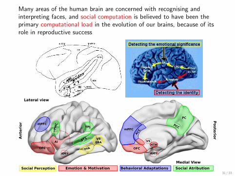
Many areas of the human brain are concerned with recognising andinterpreting faces, and social computation is believed to have been theprimary computational load in the evolution of our brains, because of itsrole in reproductive success

�� !"#$%&�#��!!!!$$�!!�!!!�!��’(��)�*��

$��(�� +!�!+�!%�+#��,

�� $%��(�$�.�!�� /��

�� 0 �1��)��0��-��2��1��)��0��

��

��

��3��4�50�� (�6�� 5�� )��6��2�7��4�8 �0 ��9��:;�8��1��<��=��>��<�?��@��

, ��)�� &�� )�

��)�� ! �- ��

��)�� ! �- .��%�%

��)�� ! �- ��"

��)�� ! �- ��%��%

��)�� ! �- ��))�

��)�� %# �&�� )�

��)�� )��

��)�� ! �- ��

��)�� ! �- .��%�%

��)�� ! �- ��"

��)�� ! �- ��%��%

��)�� ! �- ��))�

31 / 33

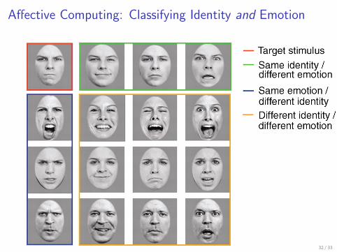
Affective Computing: Classifying Identity and Emotion

32 / 33

(Affective Computing: Interpreting Facial Emotion)

MRI scanning has revealed much about brain areas that interpret facialexpressions. Affective computing aims to classify visual emotions asarticulated sequences using Hidden Markov Models of their generation.Mapping the visible data to action sequences of the facial musculaturebecomes a generative classifier of emotions.

33 / 33

(4th supplementary slides: computer vision) · (4th supplementary slides: computer vision) ......

Documents