4b. properties of negative downward lightning discharge to ... 4b.pdf · courtesy prof. dr....
TRANSCRIPT

1
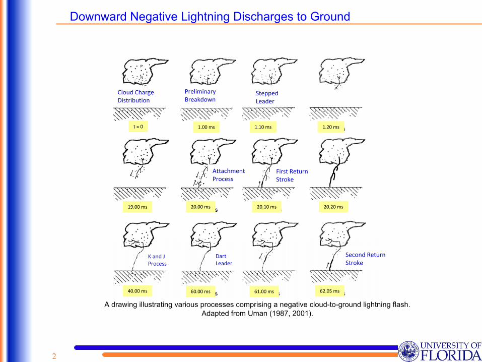
4b Properties of negative downward lightning discharge to ground - II
Cloud Charge
DistributionPreliminaryBreakdown
SteppedLeader
AttachmentProcess
First ReturnStroke
DartLeader
K and J
Process
t = 0 100 ms 110 ms 120 ms
1900 ms 2000 ms 2010 ms 2020 ms
4000 ms 6000 ms 6100 ms 6205 ms
A drawing illustrating various processes comprising a negative cloud-to-ground lightning flash Adapted from Uman
(1987 2001)
Second ReturnStroke
Downward Negative Lightning Discharges to Ground
2
(a)
Streak‐camera photograph of a lightning discharge to a tower on Monte San
Salvatore Switzerland showing evidence of an upward connecting
leader
(b)
Still photograph of the same flash and another flash that attached to the tower
below its top
Adapted from Berger and Vogelsanger
(1966)
(a)
Streak‐camera photograph of a lightning discharge to a tower on Monte San
Salvatore Switzerland showing evidence of an upward connecting
leader
(b)
Still photograph of the same flash and another flash that attached to the tower
below its top
Adapted from Berger and Vogelsanger
(1966)
Adapted from Howard (2009)5
Lightning Attachment Process
6
Optical Images of Leader and Attachment Process ndash Triggered Lightning
Dart-stepped leader and attachement
process in rocket-triggered lightning (Sept 17 2008) at Camp Blanding Florida Photron
FASTCAM SA11 50000 fps (20 micros per frame)
Biagi
et al (2009 GRL)2 frames before return stroke 8 1 frame before return stroke 8
56 m
16 m
25 m
7
Optical Images of Leader and Attachment Process ndash Laboratory Sparks
Single-frame K008 images of four negative discharges (-22 MV1307500 μs) in a 45 m rod-rod gap Frame duration in a b and c is 2 micros and in d it is 05 micros L in b is the length of last step Adapted from Lebedev et al (2007)
-4
5 m
8
Optical Images of Attachment Process
55
m
HV rod
JP
Single-frame image-converter-camera K008 images of negative discharges in a 55-m rod-rod gap with frame exposure of 02 μs JP is the junction point between downward negative and upward connecting positive leaders Adapted from
Shcherbakov
et al (2006)
A photograph of a lightning strike to a chimney pot showing a split in the channel interpreted as evidence of an upward connecting leader Adapted from Golde
(1967)
JP
9
Illustration of capture surfaces of two towers and earthrsquos surface in the electrogeometrical
model (EGM) rs
is the striking distance defined as the distance from the tip of the descending leader to the object to be struck at the instant when an upward connecting leader is initiated from this object
Vertical arrows represent descending leaders assumed to be uniformly distributed (Ng=const) above the capture surfaces Adapted from Bazelyan
and Raizer
(2000)
Electrogeometrical Model (EGM)
rs
rsrs
Capture surfaces
Ng=const
10
Electrogeometrical Model (EGM)
rs
= 10 I065 m where I
is in kA
4
3
12
Striking distance rs
versus return-stroke peak current I
[curve 1 Golde
(1945) curve 2 Wagner (1963) curve 3 Love (1973) curve 4 Ruhling
(1972) x theory of Davis (1962) estimates from two-
dimensional photographs by Eriksson (1978) estimates from three-dimensional photography by Eriksson (1978) Adapted from Golde
(1977) and Eriksson (1978)
I kA rs m
10 45
30 91
170 282
11
Scatter plot of impulse charge Q versus return-stroke peak current
I Note that both vertical and horizontal scales are logarithmic The best fit to data I
= 106 Q07 where Q is in coulombs and I
is in kiloamperes was used in deriving rs
= 10 I065
Adapted from Berger (1972)
Electrogeometrical Model (EGM)
Finding rs = f(I)
bull
Assume critical average electric field between the leader tip and the strike object at the time of initiation of upward connecting leader from the object (200-600 kVm)
bull
Use an empirical relation between Q and I
to find rs
= f(I)
bull
Find rs
= f(Q)
bull
Assume leader geometry total leader charge Q and distribution of this charge along the channel
Q
10-1
100
101
102
100 101 102I
I
peak Q impulseneg first strokes n=89
I
= 106 Q07
For Q = 5 CI
= 33 kA
12
Electrogeometrical Model (EGM)
Illustration of the rolling-sphere method (RSM) The shaded area is that area into which it is postulated lightning cannot enter Adapted from Szczerbinski
(2000)
rs
rsrs
rs = 45 m (150 ft) (NFPA 780 2004) corresponds to I
= 10 kA (95 of currents exceed this value)
Rolling-Sphere Method
Return‐Stroke Fields Variation with Distance
Typical vertical electric field intensity (left column) and azimuthal
magnetic flux density (right column) waveforms for first (solid line) and subsequent (dashed line) return strokes at distances of 1 2 and 5 km Adapted from Lin et al (1979)
Electric Field Intensity Magnetic Flux Density
Return‐Stroke Fields Variation with Distance
Electric Field IntensityMagnetic Flux Density
Typical vertical electric field intensity (left column) and azimuthal
magnetic flux density (right column) waveforms for first (solid line) and subsequent (dashed line) return strokes at distances of 10 15 50 and 200 km Adapted from Lin et al (1979)
Return-Stroke Current Waveshapes
ndash
Switzerland (Berger et al 1975)
15
Average negative first and subsequent-stroke current waveshapes
each shown on two time scales A
and B The lower time scales (A) correspond to the solid curves while the upper time scales (B) correspond to the broken curves The vertical (amplitude) scale is in relative units the peak values being equal to negative unity Adapted from Berger et al (1975)
Lightning Parameters Derived from Direct Current Measurements
Parameters Units Sample Size
Percent Exceeding Tabulated Value
95 50 5
Peak current
(minimum 2 kA)First strokesSubsequent strokes
kA 101135
1446
3012
8030
Charge
(total charge)First strokesSubsequent strokesComplete flash
C 9312294
110213
521475
241140
Impulse charge
(excluding continuing current)
First strokesSubsequent strokes
C90
11711
02245
09520
4Front duration
(2 kA to peak)First strokesSubsequent strokes
μs 89118
18022
5511
1845
Maximum dIdtFirst strokesSubsequent strokes
kA μs-1 92122
5512
1240
32120
Stroke duration
(2 kA to half peak value on the tail)
First strokesSubsequent strokes
μs90
1153065
7532
200140
Action integral (intI2dt)First strokesSubsequent strokes
A2s 9188
60 x 103
55 x 10255 x 104
60 x 10355 x 105
52 x 104
17
Cumulative statistical distributions of lightning peak currents
giving percent of cases exceeding abscissa value from direct measurements in Switzerland (Berger 1972 Berger et al 1975) The distributions are assumed to be lognormal and given for (1) negative first strokes (2) positive first strokes (3) negative and positive first strokes and (4) negative subsequent strokes Adapted from Bazelyan
et al (1978)
Lightning peak currents for first strokes vary by a factor of 50 or more from about 5 to 250 kA
The probability of occurrence of a given value rapidly increases up to 25 kA
or so and then slowly decreasesStatistical distributions of this type are often assumed to be lognormal
Lightning Peak Current ndash
Bergerrsquos Distributions
18
Cumulative statistical distributions of peak currents (percent values on the vertical axis should be subtracted from 100 to obtain the probability to exceed the peak current value on the horizontal axis) for negative first strokes adopted by IEEE
and CIGRE Taken from CIGRE Document 63 (1991)
For the CIGRE
distribution 98 of peak currents exceed 4 kA 80 exceed 20 kA and 5 exceed 90 kA
For the IEEE
distribution the ldquoprobability to exceedrdquo
values are given by the following equation
where PI
is in per unit and I is in kA This equation applies to values of I up to 200 kA The median (50) peak current value is equal to 31 kA
Peak current I kA(IEEE
distribution) 5 10 20 40 60 80 100 200
Percentage exceeding tabulated value PI
10099 95 76 34 15 78 45 08
( ) 62
311
1I
PI+
=
Lightning Peak Current ndash
IEEE and CIGRE Distributions
dIdt
in Rocket-Triggered Lightning ( ~100 kAμs)
19
Relation between the peak rate of current rise dIdt and the peak current I from triggered-lightning experiments conducted at the NASA Kennedy Space Center Florida in 19851987 and 1988 and in France in 1986 The regression line for each year is shown the sample size N and the regression equation are given in table Adapted from Leteinturier
et al (1991)
Morro Do Cachimbo
Tower (60 m) Belo Horizonte Brazil
20
Courtesy Prof Dr Silverio Visacro Filho Lightning Research Center (UFMG-CEMIG)
Lightning Parameters Derived from Direct Current Measurements ndash
Brazil
21
First Stroke
Subsequent Strokes
404
52
163
099
Optical Measurements of Return-Stroke Speed
22
Optical intensity (in millivolts
at the input of the oscilloscope) vs time waveforms at four different heights 7 63 117 and 170 m
above the lightning termination point for stroke 1 in flash F0336 Adapted from Olsen et al (2004)
23
Reference St Dev ms Comments
Natural Lightning
Boyle and Orville (1976)
20 x 107 12 x 108 071 x 108 26 x 107 12 Streak camera 2-D speed
Idone and Orville (1982)
29 x 107 24 x 108 11 x 108 47 x 107 63 Streak camera2-D speed
Mach and Rust (1989a Fig 7)
20 x 107
80 x 10726 x 108
gt28 x 1085 x 107
7 x 1075443
Long channelShort channel (Photoelectric 2-D)
Triggered Lightning
Hubert and Mouget (1981)
45 x 107 17 x 108 99 x 107 41 x 107 13 Photoelectric3-D speed
Idone et al (1984) 67 x 107 17 x 108 12 x 108 27 x 107 56 Streak camera 3-D speed
Willett et al (1988)
10 x 108 15 x 108 12 x 108 16 x 107 9 Streak camera 2-D speed
Willett et al (1989a)
12 x 108 19 x 108 15 x 108 17 x 107 18 Streak camera 2-D speed
Mach and Rust (1989a Fig 8)
60 x 107
60 x 10716 x 108
20 x 1082 x 107
4 x 1074039
Long channelShort channel(Photoelectric 2-D)
Min ms Max ms Mean ms Sample
Size
13 plusmn03 x 108
19 plusmn07 x 108
12 plusmn03 x 108
14 plusmn04 x 108
Summary of measured return stroke speeds averaged over the visible part of the channel in natural and triggered negative lightning Adapted from Rakov
et al (1992b)
Return-Stroke Speed Near Ground
24
Height Above Ground
7-63 m
63-117 m
117-170
m
12
16
15
12121213
18
16
16
17
18 18
1512
Return-stroke speed profiles estimated tracking the 20 point on the light-pulse front for triggered lightning flash F0336 (Olsen et al 2004)
Return-Stroke Speed vs Return-Stroke Peak Current
25
Return-stroke speed vs peak current for 29 triggered-lightning strokes observed at the Kennedy Space Center (KSC) Florida in 1986 and reported by Mach and Rust (1989a) and 18 triggered-lightning strokes from the 1987 KSC experiments reported by Willett et al
(1989a) Peak curent shown in the scatter plot as 38 kA may be an underestimate Note that the linear correlation coefficients (r) for both data sets are low and negative not in support of the often assumed relationship between these two lightning parameters
00
05
10
15
20
25
0 5 10 15 20 25 30 35 40 45
Return-Stroke Peak Current kA
Ret
urn-
Stro
ke S
peed
108 m
s
Mach and Rust (1989a) r = -008
Willett el al (1998a) r = -027
First Return Stroke
Electric field waveforms of a first return stroke The waveform is shown on two time scales 5 μsdiv
and 10 μsdiv The fields are normalized to a distance of 100 km L denotes individual leader pulses F slow front and R fast transition Also marked are the small secondary peak or shoulder α
and the larger subsidiary peaks a b and c Adapted from Weidman and Krider
(1978)
-20 -15 -10 -5 0 5 10 15 20
5
microsdiv
10
microsdiv
-60 -40 -20 0 20 40 60 80
26
Subsequent Return Strokes
-20 -15 -10 -5 0 5 10 15 20
5 microsdiv
5 microsdiv
10 microsdiv
10 microsdiv
-60 -40 -20 0 20 40 60 80
Electric field waveforms of (b) a subsequent return stroke initiated by a dart-stepped leader and (c) a subsequent return stroke initiated by a dart leader showing the fine structure both before and after the initial field peak Each waveform is shown on two time scales 5 μsdiv
and 10 μsdiv The fields are normalized to a distance of 100 km L denotes individual leader pulses F slow front and R fast transition Also marked are the small secondary peak or shoulder α
and the larger subsidiary peaks a b and c Adapted from Weidman and Krider
(1978)
27
First Return Stroke Electric Field Derivative
Examples of (top) the time derivative of the electric field intensity dEdt
and (bottom)
the electric field intensity E produced by a first return stroke at a distance of about 36 km over the Atlantic Ocean The propagation path was almost entirely over salt water The vertical arrow under the E record shows the time of the dEdt
trigger Adapted from Krider
et al (1996)
28
Return Strokes Measured Parameters
Parameters of microsecond-scale electric field waveforms produced by negative return strokes
Parameter Location First strokes Subsequent strokes
Sample size Mean SD Sample size Mean SD
Initial peak (V m‐1) (normalized to 100 km)Rakov
and Uman
(1990b)
Cooray
and Lundquist (1982)Lin et al (1979)
Florida
SwedenKSCOcala
76
5535129
59 (GM)
536758
273825
232a
38b
8359
27(GM)41(GM)
5043
2215
Zero‐crossing time (μs)Cooray
and Lundquist (1985)
Lin et al (1979)
SwedenSri LankaFlorida
1029146c
498954
123018
9414377c
394236
81417
Zero‐to‐peak rise time (μs)Master et al (1984)Cooray
and Lundquist (1982)Lin et al (1979)
FloridaSwedenKSCOcala
1051405129
44702427
18201213
220
8359
28
1519
15
0807
10‐90 percent rise time (μs)Master et al (1984) Florida 105 26 12 220 15 09
Slow front duration
(μs)Master et al (1984)Cooray
and Lundquist (1982)Weidman and Krider
(1978)
FloridaSwedenFlorida
105826290
29504041
13201716
44 120 34d
060921
020509
29
Return Strokes Measured ParametersParameters of microsecond-scale electric field waveforms produced by negative return strokes (contrsquod)
Parameter Locatio
nFirst strokes Subsequent strokes
Sample size
Mean SD Sample size Mean SD
Slow front amplitude as percentage of peakMaster et al (1984)Cooray
and Lundquist (1982)Weidman and Krider
(1978)
FloridaSwedenFlorida
105836290
28415040
15112020
4412034d
202540
101020
Fast
transition 10-90 percent risetime
(ns)Master et al (1984)Weidman and Krider
(1978)
Weidman and Krider
(1980a 1984)
Weidman (1982)
FloridaFlorida
Florida
1023815125
97020020090
68010010040
2178034
610200150
27040100
Peak time derivative (normalized to100 km ) (V m-1
μs-1)Krider
et al (1996) Florida 63 39 11
Time derivative pulse width at half-peak value (ns)
Krider
et al (1996) Florida 61 100 20
If not specicied
otherwise multiple lines for a given source for the same location correspond to different thunderstorms GM = geometric mean value a better characteristic of the distribution of initial field peaks since this distribution is approximately log-normala
Strokes following previously formed channelb
Strokes creating new termination on groundcBoth
electric and magnetic fieldsd
Subsequent strokes initiated by dart-stepped leaders Other subsequent strokes studied by Weidman and
Krider
(1978) were initiated by dart leaders
30
- Slide Number 1
- Slide Number 2
- Slide Number 3
- Slide Number 4
- Slide Number 5
- Slide Number 6
- Slide Number 7
- Slide Number 8
- Slide Number 9
- Slide Number 10
- Slide Number 11
- Slide Number 12
- Return-Stroke Fields Variation with Distance
- Return-Stroke Fields Variation with Distance
- Slide Number 15
- Slide Number 16
- Slide Number 17
- Slide Number 18
- Slide Number 19
- Slide Number 20
- Slide Number 21
- Slide Number 22
- Slide Number 23
- Slide Number 24
- Slide Number 25
- First Return Stroke
- Subsequent Return Strokes
- First Return Stroke Electric Field Derivative
- Return Strokes Measured Parameters
- Return Strokes Measured Parameters
-

(a)
Streak‐camera photograph of a lightning discharge to a tower on Monte San
Salvatore Switzerland showing evidence of an upward connecting
leader
(b)
Still photograph of the same flash and another flash that attached to the tower
below its top
Adapted from Berger and Vogelsanger
(1966)
(a)
Streak‐camera photograph of a lightning discharge to a tower on Monte San
Salvatore Switzerland showing evidence of an upward connecting
leader
(b)
Still photograph of the same flash and another flash that attached to the tower
below its top
Adapted from Berger and Vogelsanger
(1966)
Adapted from Howard (2009)5
Lightning Attachment Process
6
Optical Images of Leader and Attachment Process ndash Triggered Lightning
Dart-stepped leader and attachement
process in rocket-triggered lightning (Sept 17 2008) at Camp Blanding Florida Photron
FASTCAM SA11 50000 fps (20 micros per frame)
Biagi
et al (2009 GRL)2 frames before return stroke 8 1 frame before return stroke 8
56 m
16 m
25 m
7
Optical Images of Leader and Attachment Process ndash Laboratory Sparks
Single-frame K008 images of four negative discharges (-22 MV1307500 μs) in a 45 m rod-rod gap Frame duration in a b and c is 2 micros and in d it is 05 micros L in b is the length of last step Adapted from Lebedev et al (2007)
-4
5 m
8
Optical Images of Attachment Process
55
m
HV rod
JP
Single-frame image-converter-camera K008 images of negative discharges in a 55-m rod-rod gap with frame exposure of 02 μs JP is the junction point between downward negative and upward connecting positive leaders Adapted from
Shcherbakov
et al (2006)
A photograph of a lightning strike to a chimney pot showing a split in the channel interpreted as evidence of an upward connecting leader Adapted from Golde
(1967)
JP
9
Illustration of capture surfaces of two towers and earthrsquos surface in the electrogeometrical
model (EGM) rs
is the striking distance defined as the distance from the tip of the descending leader to the object to be struck at the instant when an upward connecting leader is initiated from this object
Vertical arrows represent descending leaders assumed to be uniformly distributed (Ng=const) above the capture surfaces Adapted from Bazelyan
and Raizer
(2000)
Electrogeometrical Model (EGM)
rs
rsrs
Capture surfaces
Ng=const
10
Electrogeometrical Model (EGM)
rs
= 10 I065 m where I
is in kA
4
3
12
Striking distance rs
versus return-stroke peak current I
[curve 1 Golde
(1945) curve 2 Wagner (1963) curve 3 Love (1973) curve 4 Ruhling
(1972) x theory of Davis (1962) estimates from two-
dimensional photographs by Eriksson (1978) estimates from three-dimensional photography by Eriksson (1978) Adapted from Golde
(1977) and Eriksson (1978)
I kA rs m
10 45
30 91
170 282
11
Scatter plot of impulse charge Q versus return-stroke peak current
I Note that both vertical and horizontal scales are logarithmic The best fit to data I
= 106 Q07 where Q is in coulombs and I
is in kiloamperes was used in deriving rs
= 10 I065
Adapted from Berger (1972)
Electrogeometrical Model (EGM)
Finding rs = f(I)
bull
Assume critical average electric field between the leader tip and the strike object at the time of initiation of upward connecting leader from the object (200-600 kVm)
bull
Use an empirical relation between Q and I
to find rs
= f(I)
bull
Find rs
= f(Q)
bull
Assume leader geometry total leader charge Q and distribution of this charge along the channel
Q
10-1
100
101
102
100 101 102I
I
peak Q impulseneg first strokes n=89
I
= 106 Q07
For Q = 5 CI
= 33 kA
12
Electrogeometrical Model (EGM)
Illustration of the rolling-sphere method (RSM) The shaded area is that area into which it is postulated lightning cannot enter Adapted from Szczerbinski
(2000)
rs
rsrs
rs = 45 m (150 ft) (NFPA 780 2004) corresponds to I
= 10 kA (95 of currents exceed this value)
Rolling-Sphere Method
Return‐Stroke Fields Variation with Distance
Typical vertical electric field intensity (left column) and azimuthal
magnetic flux density (right column) waveforms for first (solid line) and subsequent (dashed line) return strokes at distances of 1 2 and 5 km Adapted from Lin et al (1979)
Electric Field Intensity Magnetic Flux Density
Return‐Stroke Fields Variation with Distance
Electric Field IntensityMagnetic Flux Density
Typical vertical electric field intensity (left column) and azimuthal
magnetic flux density (right column) waveforms for first (solid line) and subsequent (dashed line) return strokes at distances of 10 15 50 and 200 km Adapted from Lin et al (1979)
Return-Stroke Current Waveshapes
ndash
Switzerland (Berger et al 1975)
15
Average negative first and subsequent-stroke current waveshapes
each shown on two time scales A
and B The lower time scales (A) correspond to the solid curves while the upper time scales (B) correspond to the broken curves The vertical (amplitude) scale is in relative units the peak values being equal to negative unity Adapted from Berger et al (1975)
Lightning Parameters Derived from Direct Current Measurements
Parameters Units Sample Size
Percent Exceeding Tabulated Value
95 50 5
Peak current
(minimum 2 kA)First strokesSubsequent strokes
kA 101135
1446
3012
8030
Charge
(total charge)First strokesSubsequent strokesComplete flash
C 9312294
110213
521475
241140
Impulse charge
(excluding continuing current)
First strokesSubsequent strokes
C90
11711
02245
09520
4Front duration
(2 kA to peak)First strokesSubsequent strokes
μs 89118
18022
5511
1845
Maximum dIdtFirst strokesSubsequent strokes
kA μs-1 92122
5512
1240
32120
Stroke duration
(2 kA to half peak value on the tail)
First strokesSubsequent strokes
μs90
1153065
7532
200140
Action integral (intI2dt)First strokesSubsequent strokes
A2s 9188
60 x 103
55 x 10255 x 104
60 x 10355 x 105
52 x 104
17
Cumulative statistical distributions of lightning peak currents
giving percent of cases exceeding abscissa value from direct measurements in Switzerland (Berger 1972 Berger et al 1975) The distributions are assumed to be lognormal and given for (1) negative first strokes (2) positive first strokes (3) negative and positive first strokes and (4) negative subsequent strokes Adapted from Bazelyan
et al (1978)
Lightning peak currents for first strokes vary by a factor of 50 or more from about 5 to 250 kA
The probability of occurrence of a given value rapidly increases up to 25 kA
or so and then slowly decreasesStatistical distributions of this type are often assumed to be lognormal
Lightning Peak Current ndash
Bergerrsquos Distributions
18
Cumulative statistical distributions of peak currents (percent values on the vertical axis should be subtracted from 100 to obtain the probability to exceed the peak current value on the horizontal axis) for negative first strokes adopted by IEEE
and CIGRE Taken from CIGRE Document 63 (1991)
For the CIGRE
distribution 98 of peak currents exceed 4 kA 80 exceed 20 kA and 5 exceed 90 kA
For the IEEE
distribution the ldquoprobability to exceedrdquo
values are given by the following equation
where PI
is in per unit and I is in kA This equation applies to values of I up to 200 kA The median (50) peak current value is equal to 31 kA
Peak current I kA(IEEE
distribution) 5 10 20 40 60 80 100 200
Percentage exceeding tabulated value PI
10099 95 76 34 15 78 45 08
( ) 62
311
1I
PI+
=
Lightning Peak Current ndash
IEEE and CIGRE Distributions
dIdt
in Rocket-Triggered Lightning ( ~100 kAμs)
19
Relation between the peak rate of current rise dIdt and the peak current I from triggered-lightning experiments conducted at the NASA Kennedy Space Center Florida in 19851987 and 1988 and in France in 1986 The regression line for each year is shown the sample size N and the regression equation are given in table Adapted from Leteinturier
et al (1991)
Morro Do Cachimbo
Tower (60 m) Belo Horizonte Brazil
20
Courtesy Prof Dr Silverio Visacro Filho Lightning Research Center (UFMG-CEMIG)
Lightning Parameters Derived from Direct Current Measurements ndash
Brazil
21
First Stroke
Subsequent Strokes
404
52
163
099
Optical Measurements of Return-Stroke Speed
22
Optical intensity (in millivolts
at the input of the oscilloscope) vs time waveforms at four different heights 7 63 117 and 170 m
above the lightning termination point for stroke 1 in flash F0336 Adapted from Olsen et al (2004)
23
Reference St Dev ms Comments
Natural Lightning
Boyle and Orville (1976)
20 x 107 12 x 108 071 x 108 26 x 107 12 Streak camera 2-D speed
Idone and Orville (1982)
29 x 107 24 x 108 11 x 108 47 x 107 63 Streak camera2-D speed
Mach and Rust (1989a Fig 7)
20 x 107
80 x 10726 x 108
gt28 x 1085 x 107
7 x 1075443
Long channelShort channel (Photoelectric 2-D)
Triggered Lightning
Hubert and Mouget (1981)
45 x 107 17 x 108 99 x 107 41 x 107 13 Photoelectric3-D speed
Idone et al (1984) 67 x 107 17 x 108 12 x 108 27 x 107 56 Streak camera 3-D speed
Willett et al (1988)
10 x 108 15 x 108 12 x 108 16 x 107 9 Streak camera 2-D speed
Willett et al (1989a)
12 x 108 19 x 108 15 x 108 17 x 107 18 Streak camera 2-D speed
Mach and Rust (1989a Fig 8)
60 x 107
60 x 10716 x 108
20 x 1082 x 107
4 x 1074039
Long channelShort channel(Photoelectric 2-D)
Min ms Max ms Mean ms Sample
Size
13 plusmn03 x 108
19 plusmn07 x 108
12 plusmn03 x 108
14 plusmn04 x 108
Summary of measured return stroke speeds averaged over the visible part of the channel in natural and triggered negative lightning Adapted from Rakov
et al (1992b)
Return-Stroke Speed Near Ground
24
Height Above Ground
7-63 m
63-117 m
117-170
m
12
16
15
12121213
18
16
16
17
18 18
1512
Return-stroke speed profiles estimated tracking the 20 point on the light-pulse front for triggered lightning flash F0336 (Olsen et al 2004)
Return-Stroke Speed vs Return-Stroke Peak Current
25
Return-stroke speed vs peak current for 29 triggered-lightning strokes observed at the Kennedy Space Center (KSC) Florida in 1986 and reported by Mach and Rust (1989a) and 18 triggered-lightning strokes from the 1987 KSC experiments reported by Willett et al
(1989a) Peak curent shown in the scatter plot as 38 kA may be an underestimate Note that the linear correlation coefficients (r) for both data sets are low and negative not in support of the often assumed relationship between these two lightning parameters
00
05
10
15
20
25
0 5 10 15 20 25 30 35 40 45
Return-Stroke Peak Current kA
Ret
urn-
Stro
ke S
peed
108 m
s
Mach and Rust (1989a) r = -008
Willett el al (1998a) r = -027
First Return Stroke
Electric field waveforms of a first return stroke The waveform is shown on two time scales 5 μsdiv
and 10 μsdiv The fields are normalized to a distance of 100 km L denotes individual leader pulses F slow front and R fast transition Also marked are the small secondary peak or shoulder α
and the larger subsidiary peaks a b and c Adapted from Weidman and Krider
(1978)
-20 -15 -10 -5 0 5 10 15 20
5
microsdiv
10
microsdiv
-60 -40 -20 0 20 40 60 80
26
Subsequent Return Strokes
-20 -15 -10 -5 0 5 10 15 20
5 microsdiv
5 microsdiv
10 microsdiv
10 microsdiv
-60 -40 -20 0 20 40 60 80
Electric field waveforms of (b) a subsequent return stroke initiated by a dart-stepped leader and (c) a subsequent return stroke initiated by a dart leader showing the fine structure both before and after the initial field peak Each waveform is shown on two time scales 5 μsdiv
and 10 μsdiv The fields are normalized to a distance of 100 km L denotes individual leader pulses F slow front and R fast transition Also marked are the small secondary peak or shoulder α
and the larger subsidiary peaks a b and c Adapted from Weidman and Krider
(1978)
27
First Return Stroke Electric Field Derivative
Examples of (top) the time derivative of the electric field intensity dEdt
and (bottom)
the electric field intensity E produced by a first return stroke at a distance of about 36 km over the Atlantic Ocean The propagation path was almost entirely over salt water The vertical arrow under the E record shows the time of the dEdt
trigger Adapted from Krider
et al (1996)
28
Return Strokes Measured Parameters
Parameters of microsecond-scale electric field waveforms produced by negative return strokes
Parameter Location First strokes Subsequent strokes
Sample size Mean SD Sample size Mean SD
Initial peak (V m‐1) (normalized to 100 km)Rakov
and Uman
(1990b)
Cooray
and Lundquist (1982)Lin et al (1979)
Florida
SwedenKSCOcala
76
5535129
59 (GM)
536758
273825
232a
38b
8359
27(GM)41(GM)
5043
2215
Zero‐crossing time (μs)Cooray
and Lundquist (1985)
Lin et al (1979)
SwedenSri LankaFlorida
1029146c
498954
123018
9414377c
394236
81417
Zero‐to‐peak rise time (μs)Master et al (1984)Cooray
and Lundquist (1982)Lin et al (1979)
FloridaSwedenKSCOcala
1051405129
44702427
18201213
220
8359
28
1519
15
0807
10‐90 percent rise time (μs)Master et al (1984) Florida 105 26 12 220 15 09
Slow front duration
(μs)Master et al (1984)Cooray
and Lundquist (1982)Weidman and Krider
(1978)
FloridaSwedenFlorida
105826290
29504041
13201716
44 120 34d
060921
020509
29
Return Strokes Measured ParametersParameters of microsecond-scale electric field waveforms produced by negative return strokes (contrsquod)
Parameter Locatio
nFirst strokes Subsequent strokes
Sample size
Mean SD Sample size Mean SD
Slow front amplitude as percentage of peakMaster et al (1984)Cooray
and Lundquist (1982)Weidman and Krider
(1978)
FloridaSwedenFlorida
105836290
28415040
15112020
4412034d
202540
101020
Fast
transition 10-90 percent risetime
(ns)Master et al (1984)Weidman and Krider
(1978)
Weidman and Krider
(1980a 1984)
Weidman (1982)
FloridaFlorida
Florida
1023815125
97020020090
68010010040
2178034
610200150
27040100
Peak time derivative (normalized to100 km ) (V m-1
μs-1)Krider
et al (1996) Florida 63 39 11
Time derivative pulse width at half-peak value (ns)
Krider
et al (1996) Florida 61 100 20
If not specicied
otherwise multiple lines for a given source for the same location correspond to different thunderstorms GM = geometric mean value a better characteristic of the distribution of initial field peaks since this distribution is approximately log-normala
Strokes following previously formed channelb
Strokes creating new termination on groundcBoth
electric and magnetic fieldsd
Subsequent strokes initiated by dart-stepped leaders Other subsequent strokes studied by Weidman and
Krider
(1978) were initiated by dart leaders
30
- Slide Number 1
- Slide Number 2
- Slide Number 3
- Slide Number 4
- Slide Number 5
- Slide Number 6
- Slide Number 7
- Slide Number 8
- Slide Number 9
- Slide Number 10
- Slide Number 11
- Slide Number 12
- Return-Stroke Fields Variation with Distance
- Return-Stroke Fields Variation with Distance
- Slide Number 15
- Slide Number 16
- Slide Number 17
- Slide Number 18
- Slide Number 19
- Slide Number 20
- Slide Number 21
- Slide Number 22
- Slide Number 23
- Slide Number 24
- Slide Number 25
- First Return Stroke
- Subsequent Return Strokes
- First Return Stroke Electric Field Derivative
- Return Strokes Measured Parameters
- Return Strokes Measured Parameters
-

(a)
Streak‐camera photograph of a lightning discharge to a tower on Monte San
Salvatore Switzerland showing evidence of an upward connecting
leader
(b)
Still photograph of the same flash and another flash that attached to the tower
below its top
Adapted from Berger and Vogelsanger
(1966)
Adapted from Howard (2009)5
Lightning Attachment Process
6
Optical Images of Leader and Attachment Process ndash Triggered Lightning
Dart-stepped leader and attachement
process in rocket-triggered lightning (Sept 17 2008) at Camp Blanding Florida Photron
FASTCAM SA11 50000 fps (20 micros per frame)
Biagi
et al (2009 GRL)2 frames before return stroke 8 1 frame before return stroke 8
56 m
16 m
25 m
7
Optical Images of Leader and Attachment Process ndash Laboratory Sparks
Single-frame K008 images of four negative discharges (-22 MV1307500 μs) in a 45 m rod-rod gap Frame duration in a b and c is 2 micros and in d it is 05 micros L in b is the length of last step Adapted from Lebedev et al (2007)
-4
5 m
8
Optical Images of Attachment Process
55
m
HV rod
JP
Single-frame image-converter-camera K008 images of negative discharges in a 55-m rod-rod gap with frame exposure of 02 μs JP is the junction point between downward negative and upward connecting positive leaders Adapted from
Shcherbakov
et al (2006)
A photograph of a lightning strike to a chimney pot showing a split in the channel interpreted as evidence of an upward connecting leader Adapted from Golde
(1967)
JP
9
Illustration of capture surfaces of two towers and earthrsquos surface in the electrogeometrical
model (EGM) rs
is the striking distance defined as the distance from the tip of the descending leader to the object to be struck at the instant when an upward connecting leader is initiated from this object
Vertical arrows represent descending leaders assumed to be uniformly distributed (Ng=const) above the capture surfaces Adapted from Bazelyan
and Raizer
(2000)
Electrogeometrical Model (EGM)
rs
rsrs
Capture surfaces
Ng=const
10
Electrogeometrical Model (EGM)
rs
= 10 I065 m where I
is in kA
4
3
12
Striking distance rs
versus return-stroke peak current I
[curve 1 Golde
(1945) curve 2 Wagner (1963) curve 3 Love (1973) curve 4 Ruhling
(1972) x theory of Davis (1962) estimates from two-
dimensional photographs by Eriksson (1978) estimates from three-dimensional photography by Eriksson (1978) Adapted from Golde
(1977) and Eriksson (1978)
I kA rs m
10 45
30 91
170 282
11
Scatter plot of impulse charge Q versus return-stroke peak current
I Note that both vertical and horizontal scales are logarithmic The best fit to data I
= 106 Q07 where Q is in coulombs and I
is in kiloamperes was used in deriving rs
= 10 I065
Adapted from Berger (1972)
Electrogeometrical Model (EGM)
Finding rs = f(I)
bull
Assume critical average electric field between the leader tip and the strike object at the time of initiation of upward connecting leader from the object (200-600 kVm)
bull
Use an empirical relation between Q and I
to find rs
= f(I)
bull
Find rs
= f(Q)
bull
Assume leader geometry total leader charge Q and distribution of this charge along the channel
Q
10-1
100
101
102
100 101 102I
I
peak Q impulseneg first strokes n=89
I
= 106 Q07
For Q = 5 CI
= 33 kA
12
Electrogeometrical Model (EGM)
Illustration of the rolling-sphere method (RSM) The shaded area is that area into which it is postulated lightning cannot enter Adapted from Szczerbinski
(2000)
rs
rsrs
rs = 45 m (150 ft) (NFPA 780 2004) corresponds to I
= 10 kA (95 of currents exceed this value)
Rolling-Sphere Method
Return‐Stroke Fields Variation with Distance
Typical vertical electric field intensity (left column) and azimuthal
magnetic flux density (right column) waveforms for first (solid line) and subsequent (dashed line) return strokes at distances of 1 2 and 5 km Adapted from Lin et al (1979)
Electric Field Intensity Magnetic Flux Density
Return‐Stroke Fields Variation with Distance
Electric Field IntensityMagnetic Flux Density
Typical vertical electric field intensity (left column) and azimuthal
magnetic flux density (right column) waveforms for first (solid line) and subsequent (dashed line) return strokes at distances of 10 15 50 and 200 km Adapted from Lin et al (1979)
Return-Stroke Current Waveshapes
ndash
Switzerland (Berger et al 1975)
15
Average negative first and subsequent-stroke current waveshapes
each shown on two time scales A
and B The lower time scales (A) correspond to the solid curves while the upper time scales (B) correspond to the broken curves The vertical (amplitude) scale is in relative units the peak values being equal to negative unity Adapted from Berger et al (1975)
Lightning Parameters Derived from Direct Current Measurements
Parameters Units Sample Size
Percent Exceeding Tabulated Value
95 50 5
Peak current
(minimum 2 kA)First strokesSubsequent strokes
kA 101135
1446
3012
8030
Charge
(total charge)First strokesSubsequent strokesComplete flash
C 9312294
110213
521475
241140
Impulse charge
(excluding continuing current)
First strokesSubsequent strokes
C90
11711
02245
09520
4Front duration
(2 kA to peak)First strokesSubsequent strokes
μs 89118
18022
5511
1845
Maximum dIdtFirst strokesSubsequent strokes
kA μs-1 92122
5512
1240
32120
Stroke duration
(2 kA to half peak value on the tail)
First strokesSubsequent strokes
μs90
1153065
7532
200140
Action integral (intI2dt)First strokesSubsequent strokes
A2s 9188
60 x 103
55 x 10255 x 104
60 x 10355 x 105
52 x 104
17
Cumulative statistical distributions of lightning peak currents
giving percent of cases exceeding abscissa value from direct measurements in Switzerland (Berger 1972 Berger et al 1975) The distributions are assumed to be lognormal and given for (1) negative first strokes (2) positive first strokes (3) negative and positive first strokes and (4) negative subsequent strokes Adapted from Bazelyan
et al (1978)
Lightning peak currents for first strokes vary by a factor of 50 or more from about 5 to 250 kA
The probability of occurrence of a given value rapidly increases up to 25 kA
or so and then slowly decreasesStatistical distributions of this type are often assumed to be lognormal
Lightning Peak Current ndash
Bergerrsquos Distributions
18
Cumulative statistical distributions of peak currents (percent values on the vertical axis should be subtracted from 100 to obtain the probability to exceed the peak current value on the horizontal axis) for negative first strokes adopted by IEEE
and CIGRE Taken from CIGRE Document 63 (1991)
For the CIGRE
distribution 98 of peak currents exceed 4 kA 80 exceed 20 kA and 5 exceed 90 kA
For the IEEE
distribution the ldquoprobability to exceedrdquo
values are given by the following equation
where PI
is in per unit and I is in kA This equation applies to values of I up to 200 kA The median (50) peak current value is equal to 31 kA
Peak current I kA(IEEE
distribution) 5 10 20 40 60 80 100 200
Percentage exceeding tabulated value PI
10099 95 76 34 15 78 45 08
( ) 62
311
1I
PI+
=
Lightning Peak Current ndash
IEEE and CIGRE Distributions
dIdt
in Rocket-Triggered Lightning ( ~100 kAμs)
19
Relation between the peak rate of current rise dIdt and the peak current I from triggered-lightning experiments conducted at the NASA Kennedy Space Center Florida in 19851987 and 1988 and in France in 1986 The regression line for each year is shown the sample size N and the regression equation are given in table Adapted from Leteinturier
et al (1991)
Morro Do Cachimbo
Tower (60 m) Belo Horizonte Brazil
20
Courtesy Prof Dr Silverio Visacro Filho Lightning Research Center (UFMG-CEMIG)
Lightning Parameters Derived from Direct Current Measurements ndash
Brazil
21
First Stroke
Subsequent Strokes
404
52
163
099
Optical Measurements of Return-Stroke Speed
22
Optical intensity (in millivolts
at the input of the oscilloscope) vs time waveforms at four different heights 7 63 117 and 170 m
above the lightning termination point for stroke 1 in flash F0336 Adapted from Olsen et al (2004)
23
Reference St Dev ms Comments
Natural Lightning
Boyle and Orville (1976)
20 x 107 12 x 108 071 x 108 26 x 107 12 Streak camera 2-D speed
Idone and Orville (1982)
29 x 107 24 x 108 11 x 108 47 x 107 63 Streak camera2-D speed
Mach and Rust (1989a Fig 7)
20 x 107
80 x 10726 x 108
gt28 x 1085 x 107
7 x 1075443
Long channelShort channel (Photoelectric 2-D)
Triggered Lightning
Hubert and Mouget (1981)
45 x 107 17 x 108 99 x 107 41 x 107 13 Photoelectric3-D speed
Idone et al (1984) 67 x 107 17 x 108 12 x 108 27 x 107 56 Streak camera 3-D speed
Willett et al (1988)
10 x 108 15 x 108 12 x 108 16 x 107 9 Streak camera 2-D speed
Willett et al (1989a)
12 x 108 19 x 108 15 x 108 17 x 107 18 Streak camera 2-D speed
Mach and Rust (1989a Fig 8)
60 x 107
60 x 10716 x 108
20 x 1082 x 107
4 x 1074039
Long channelShort channel(Photoelectric 2-D)
Min ms Max ms Mean ms Sample
Size
13 plusmn03 x 108
19 plusmn07 x 108
12 plusmn03 x 108
14 plusmn04 x 108
Summary of measured return stroke speeds averaged over the visible part of the channel in natural and triggered negative lightning Adapted from Rakov
et al (1992b)
Return-Stroke Speed Near Ground
24
Height Above Ground
7-63 m
63-117 m
117-170
m
12
16
15
12121213
18
16
16
17
18 18
1512
Return-stroke speed profiles estimated tracking the 20 point on the light-pulse front for triggered lightning flash F0336 (Olsen et al 2004)
Return-Stroke Speed vs Return-Stroke Peak Current
25
Return-stroke speed vs peak current for 29 triggered-lightning strokes observed at the Kennedy Space Center (KSC) Florida in 1986 and reported by Mach and Rust (1989a) and 18 triggered-lightning strokes from the 1987 KSC experiments reported by Willett et al
(1989a) Peak curent shown in the scatter plot as 38 kA may be an underestimate Note that the linear correlation coefficients (r) for both data sets are low and negative not in support of the often assumed relationship between these two lightning parameters
00
05
10
15
20
25
0 5 10 15 20 25 30 35 40 45
Return-Stroke Peak Current kA
Ret
urn-
Stro
ke S
peed
108 m
s
Mach and Rust (1989a) r = -008
Willett el al (1998a) r = -027
First Return Stroke
Electric field waveforms of a first return stroke The waveform is shown on two time scales 5 μsdiv
and 10 μsdiv The fields are normalized to a distance of 100 km L denotes individual leader pulses F slow front and R fast transition Also marked are the small secondary peak or shoulder α
and the larger subsidiary peaks a b and c Adapted from Weidman and Krider
(1978)
-20 -15 -10 -5 0 5 10 15 20
5
microsdiv
10
microsdiv
-60 -40 -20 0 20 40 60 80
26
Subsequent Return Strokes
-20 -15 -10 -5 0 5 10 15 20
5 microsdiv
5 microsdiv
10 microsdiv
10 microsdiv
-60 -40 -20 0 20 40 60 80
Electric field waveforms of (b) a subsequent return stroke initiated by a dart-stepped leader and (c) a subsequent return stroke initiated by a dart leader showing the fine structure both before and after the initial field peak Each waveform is shown on two time scales 5 μsdiv
and 10 μsdiv The fields are normalized to a distance of 100 km L denotes individual leader pulses F slow front and R fast transition Also marked are the small secondary peak or shoulder α
and the larger subsidiary peaks a b and c Adapted from Weidman and Krider
(1978)
27
First Return Stroke Electric Field Derivative
Examples of (top) the time derivative of the electric field intensity dEdt
and (bottom)
the electric field intensity E produced by a first return stroke at a distance of about 36 km over the Atlantic Ocean The propagation path was almost entirely over salt water The vertical arrow under the E record shows the time of the dEdt
trigger Adapted from Krider
et al (1996)
28
Return Strokes Measured Parameters
Parameters of microsecond-scale electric field waveforms produced by negative return strokes
Parameter Location First strokes Subsequent strokes
Sample size Mean SD Sample size Mean SD
Initial peak (V m‐1) (normalized to 100 km)Rakov
and Uman
(1990b)
Cooray
and Lundquist (1982)Lin et al (1979)
Florida
SwedenKSCOcala
76
5535129
59 (GM)
536758
273825
232a
38b
8359
27(GM)41(GM)
5043
2215
Zero‐crossing time (μs)Cooray
and Lundquist (1985)
Lin et al (1979)
SwedenSri LankaFlorida
1029146c
498954
123018
9414377c
394236
81417
Zero‐to‐peak rise time (μs)Master et al (1984)Cooray
and Lundquist (1982)Lin et al (1979)
FloridaSwedenKSCOcala
1051405129
44702427
18201213
220
8359
28
1519
15
0807
10‐90 percent rise time (μs)Master et al (1984) Florida 105 26 12 220 15 09
Slow front duration
(μs)Master et al (1984)Cooray
and Lundquist (1982)Weidman and Krider
(1978)
FloridaSwedenFlorida
105826290
29504041
13201716
44 120 34d
060921
020509
29
Return Strokes Measured ParametersParameters of microsecond-scale electric field waveforms produced by negative return strokes (contrsquod)
Parameter Locatio
nFirst strokes Subsequent strokes
Sample size
Mean SD Sample size Mean SD
Slow front amplitude as percentage of peakMaster et al (1984)Cooray
and Lundquist (1982)Weidman and Krider
(1978)
FloridaSwedenFlorida
105836290
28415040
15112020
4412034d
202540
101020
Fast
transition 10-90 percent risetime
(ns)Master et al (1984)Weidman and Krider
(1978)
Weidman and Krider
(1980a 1984)
Weidman (1982)
FloridaFlorida
Florida
1023815125
97020020090
68010010040
2178034
610200150
27040100
Peak time derivative (normalized to100 km ) (V m-1
μs-1)Krider
et al (1996) Florida 63 39 11
Time derivative pulse width at half-peak value (ns)
Krider
et al (1996) Florida 61 100 20
If not specicied
otherwise multiple lines for a given source for the same location correspond to different thunderstorms GM = geometric mean value a better characteristic of the distribution of initial field peaks since this distribution is approximately log-normala
Strokes following previously formed channelb
Strokes creating new termination on groundcBoth
electric and magnetic fieldsd
Subsequent strokes initiated by dart-stepped leaders Other subsequent strokes studied by Weidman and
Krider
(1978) were initiated by dart leaders
30
- Slide Number 1
- Slide Number 2
- Slide Number 3
- Slide Number 4
- Slide Number 5
- Slide Number 6
- Slide Number 7
- Slide Number 8
- Slide Number 9
- Slide Number 10
- Slide Number 11
- Slide Number 12
- Return-Stroke Fields Variation with Distance
- Return-Stroke Fields Variation with Distance
- Slide Number 15
- Slide Number 16
- Slide Number 17
- Slide Number 18
- Slide Number 19
- Slide Number 20
- Slide Number 21
- Slide Number 22
- Slide Number 23
- Slide Number 24
- Slide Number 25
- First Return Stroke
- Subsequent Return Strokes
- First Return Stroke Electric Field Derivative
- Return Strokes Measured Parameters
- Return Strokes Measured Parameters
-

10
Electrogeometrical Model (EGM)
rs
= 10 I065 m where I
is in kA
4
3
12
Striking distance rs
versus return-stroke peak current I
[curve 1 Golde
(1945) curve 2 Wagner (1963) curve 3 Love (1973) curve 4 Ruhling
(1972) x theory of Davis (1962) estimates from two-
dimensional photographs by Eriksson (1978) estimates from three-dimensional photography by Eriksson (1978) Adapted from Golde
(1977) and Eriksson (1978)
I kA rs m
10 45
30 91
170 282
11
Scatter plot of impulse charge Q versus return-stroke peak current
I Note that both vertical and horizontal scales are logarithmic The best fit to data I
= 106 Q07 where Q is in coulombs and I
is in kiloamperes was used in deriving rs
= 10 I065
Adapted from Berger (1972)
Electrogeometrical Model (EGM)
Finding rs = f(I)
bull
Assume critical average electric field between the leader tip and the strike object at the time of initiation of upward connecting leader from the object (200-600 kVm)
bull
Use an empirical relation between Q and I
to find rs
= f(I)
bull
Find rs
= f(Q)
bull
Assume leader geometry total leader charge Q and distribution of this charge along the channel
Q
10-1
100
101
102
100 101 102I
I
peak Q impulseneg first strokes n=89
I
= 106 Q07
For Q = 5 CI
= 33 kA
12
Electrogeometrical Model (EGM)
Illustration of the rolling-sphere method (RSM) The shaded area is that area into which it is postulated lightning cannot enter Adapted from Szczerbinski
(2000)
rs
rsrs
rs = 45 m (150 ft) (NFPA 780 2004) corresponds to I
= 10 kA (95 of currents exceed this value)
Rolling-Sphere Method
Return‐Stroke Fields Variation with Distance
Typical vertical electric field intensity (left column) and azimuthal
magnetic flux density (right column) waveforms for first (solid line) and subsequent (dashed line) return strokes at distances of 1 2 and 5 km Adapted from Lin et al (1979)
Electric Field Intensity Magnetic Flux Density
Return‐Stroke Fields Variation with Distance
Electric Field IntensityMagnetic Flux Density
Typical vertical electric field intensity (left column) and azimuthal
magnetic flux density (right column) waveforms for first (solid line) and subsequent (dashed line) return strokes at distances of 10 15 50 and 200 km Adapted from Lin et al (1979)
Return-Stroke Current Waveshapes
ndash
Switzerland (Berger et al 1975)
15
Average negative first and subsequent-stroke current waveshapes
each shown on two time scales A
and B The lower time scales (A) correspond to the solid curves while the upper time scales (B) correspond to the broken curves The vertical (amplitude) scale is in relative units the peak values being equal to negative unity Adapted from Berger et al (1975)
Lightning Parameters Derived from Direct Current Measurements
Parameters Units Sample Size
Percent Exceeding Tabulated Value
95 50 5
Peak current
(minimum 2 kA)First strokesSubsequent strokes
kA 101135
1446
3012
8030
Charge
(total charge)First strokesSubsequent strokesComplete flash
C 9312294
110213
521475
241140
Impulse charge
(excluding continuing current)
First strokesSubsequent strokes
C90
11711
02245
09520
4Front duration
(2 kA to peak)First strokesSubsequent strokes
μs 89118
18022
5511
1845
Maximum dIdtFirst strokesSubsequent strokes
kA μs-1 92122
5512
1240
32120
Stroke duration
(2 kA to half peak value on the tail)
First strokesSubsequent strokes
μs90
1153065
7532
200140
Action integral (intI2dt)First strokesSubsequent strokes
A2s 9188
60 x 103
55 x 10255 x 104
60 x 10355 x 105
52 x 104
17
Cumulative statistical distributions of lightning peak currents
giving percent of cases exceeding abscissa value from direct measurements in Switzerland (Berger 1972 Berger et al 1975) The distributions are assumed to be lognormal and given for (1) negative first strokes (2) positive first strokes (3) negative and positive first strokes and (4) negative subsequent strokes Adapted from Bazelyan
et al (1978)
Lightning peak currents for first strokes vary by a factor of 50 or more from about 5 to 250 kA
The probability of occurrence of a given value rapidly increases up to 25 kA
or so and then slowly decreasesStatistical distributions of this type are often assumed to be lognormal
Lightning Peak Current ndash
Bergerrsquos Distributions
18
Cumulative statistical distributions of peak currents (percent values on the vertical axis should be subtracted from 100 to obtain the probability to exceed the peak current value on the horizontal axis) for negative first strokes adopted by IEEE
and CIGRE Taken from CIGRE Document 63 (1991)
For the CIGRE
distribution 98 of peak currents exceed 4 kA 80 exceed 20 kA and 5 exceed 90 kA
For the IEEE
distribution the ldquoprobability to exceedrdquo
values are given by the following equation
where PI
is in per unit and I is in kA This equation applies to values of I up to 200 kA The median (50) peak current value is equal to 31 kA
Peak current I kA(IEEE
distribution) 5 10 20 40 60 80 100 200
Percentage exceeding tabulated value PI
10099 95 76 34 15 78 45 08
( ) 62
311
1I
PI+
=
Lightning Peak Current ndash
IEEE and CIGRE Distributions
dIdt
in Rocket-Triggered Lightning ( ~100 kAμs)
19
Relation between the peak rate of current rise dIdt and the peak current I from triggered-lightning experiments conducted at the NASA Kennedy Space Center Florida in 19851987 and 1988 and in France in 1986 The regression line for each year is shown the sample size N and the regression equation are given in table Adapted from Leteinturier
et al (1991)
Morro Do Cachimbo
Tower (60 m) Belo Horizonte Brazil
20
Courtesy Prof Dr Silverio Visacro Filho Lightning Research Center (UFMG-CEMIG)
Lightning Parameters Derived from Direct Current Measurements ndash
Brazil
21
First Stroke
Subsequent Strokes
404
52
163
099
Optical Measurements of Return-Stroke Speed
22
Optical intensity (in millivolts
at the input of the oscilloscope) vs time waveforms at four different heights 7 63 117 and 170 m
above the lightning termination point for stroke 1 in flash F0336 Adapted from Olsen et al (2004)
23
Reference St Dev ms Comments
Natural Lightning
Boyle and Orville (1976)
20 x 107 12 x 108 071 x 108 26 x 107 12 Streak camera 2-D speed
Idone and Orville (1982)
29 x 107 24 x 108 11 x 108 47 x 107 63 Streak camera2-D speed
Mach and Rust (1989a Fig 7)
20 x 107
80 x 10726 x 108
gt28 x 1085 x 107
7 x 1075443
Long channelShort channel (Photoelectric 2-D)
Triggered Lightning
Hubert and Mouget (1981)
45 x 107 17 x 108 99 x 107 41 x 107 13 Photoelectric3-D speed
Idone et al (1984) 67 x 107 17 x 108 12 x 108 27 x 107 56 Streak camera 3-D speed
Willett et al (1988)
10 x 108 15 x 108 12 x 108 16 x 107 9 Streak camera 2-D speed
Willett et al (1989a)
12 x 108 19 x 108 15 x 108 17 x 107 18 Streak camera 2-D speed
Mach and Rust (1989a Fig 8)
60 x 107
60 x 10716 x 108
20 x 1082 x 107
4 x 1074039
Long channelShort channel(Photoelectric 2-D)
Min ms Max ms Mean ms Sample
Size
13 plusmn03 x 108
19 plusmn07 x 108
12 plusmn03 x 108
14 plusmn04 x 108
Summary of measured return stroke speeds averaged over the visible part of the channel in natural and triggered negative lightning Adapted from Rakov
et al (1992b)
Return-Stroke Speed Near Ground
24
Height Above Ground
7-63 m
63-117 m
117-170
m
12
16
15
12121213
18
16
16
17
18 18
1512
Return-stroke speed profiles estimated tracking the 20 point on the light-pulse front for triggered lightning flash F0336 (Olsen et al 2004)
Return-Stroke Speed vs Return-Stroke Peak Current
25
Return-stroke speed vs peak current for 29 triggered-lightning strokes observed at the Kennedy Space Center (KSC) Florida in 1986 and reported by Mach and Rust (1989a) and 18 triggered-lightning strokes from the 1987 KSC experiments reported by Willett et al
(1989a) Peak curent shown in the scatter plot as 38 kA may be an underestimate Note that the linear correlation coefficients (r) for both data sets are low and negative not in support of the often assumed relationship between these two lightning parameters
00
05
10
15
20
25
0 5 10 15 20 25 30 35 40 45
Return-Stroke Peak Current kA
Ret
urn-
Stro
ke S
peed
108 m
s
Mach and Rust (1989a) r = -008
Willett el al (1998a) r = -027
First Return Stroke
Electric field waveforms of a first return stroke The waveform is shown on two time scales 5 μsdiv
and 10 μsdiv The fields are normalized to a distance of 100 km L denotes individual leader pulses F slow front and R fast transition Also marked are the small secondary peak or shoulder α
and the larger subsidiary peaks a b and c Adapted from Weidman and Krider
(1978)
-20 -15 -10 -5 0 5 10 15 20
5
microsdiv
10
microsdiv
-60 -40 -20 0 20 40 60 80
26
Subsequent Return Strokes
-20 -15 -10 -5 0 5 10 15 20
5 microsdiv
5 microsdiv
10 microsdiv
10 microsdiv
-60 -40 -20 0 20 40 60 80
Electric field waveforms of (b) a subsequent return stroke initiated by a dart-stepped leader and (c) a subsequent return stroke initiated by a dart leader showing the fine structure both before and after the initial field peak Each waveform is shown on two time scales 5 μsdiv
and 10 μsdiv The fields are normalized to a distance of 100 km L denotes individual leader pulses F slow front and R fast transition Also marked are the small secondary peak or shoulder α
and the larger subsidiary peaks a b and c Adapted from Weidman and Krider
(1978)
27
First Return Stroke Electric Field Derivative
Examples of (top) the time derivative of the electric field intensity dEdt
and (bottom)
the electric field intensity E produced by a first return stroke at a distance of about 36 km over the Atlantic Ocean The propagation path was almost entirely over salt water The vertical arrow under the E record shows the time of the dEdt
trigger Adapted from Krider
et al (1996)
28
Return Strokes Measured Parameters
Parameters of microsecond-scale electric field waveforms produced by negative return strokes
Parameter Location First strokes Subsequent strokes
Sample size Mean SD Sample size Mean SD
Initial peak (V m‐1) (normalized to 100 km)Rakov
and Uman
(1990b)
Cooray
and Lundquist (1982)Lin et al (1979)
Florida
SwedenKSCOcala
76
5535129
59 (GM)
536758
273825
232a
38b
8359
27(GM)41(GM)
5043
2215
Zero‐crossing time (μs)Cooray
and Lundquist (1985)
Lin et al (1979)
SwedenSri LankaFlorida
1029146c
498954
123018
9414377c
394236
81417
Zero‐to‐peak rise time (μs)Master et al (1984)Cooray
and Lundquist (1982)Lin et al (1979)
FloridaSwedenKSCOcala
1051405129
44702427
18201213
220
8359
28
1519
15
0807
10‐90 percent rise time (μs)Master et al (1984) Florida 105 26 12 220 15 09
Slow front duration
(μs)Master et al (1984)Cooray
and Lundquist (1982)Weidman and Krider
(1978)
FloridaSwedenFlorida
105826290
29504041
13201716
44 120 34d
060921
020509
29
Return Strokes Measured ParametersParameters of microsecond-scale electric field waveforms produced by negative return strokes (contrsquod)
Parameter Locatio
nFirst strokes Subsequent strokes
Sample size
Mean SD Sample size Mean SD
Slow front amplitude as percentage of peakMaster et al (1984)Cooray
and Lundquist (1982)Weidman and Krider
(1978)
FloridaSwedenFlorida
105836290
28415040
15112020
4412034d
202540
101020
Fast
transition 10-90 percent risetime
(ns)Master et al (1984)Weidman and Krider
(1978)
Weidman and Krider
(1980a 1984)
Weidman (1982)
FloridaFlorida
Florida
1023815125
97020020090
68010010040
2178034
610200150
27040100
Peak time derivative (normalized to100 km ) (V m-1
μs-1)Krider
et al (1996) Florida 63 39 11
Time derivative pulse width at half-peak value (ns)
Krider
et al (1996) Florida 61 100 20
If not specicied
otherwise multiple lines for a given source for the same location correspond to different thunderstorms GM = geometric mean value a better characteristic of the distribution of initial field peaks since this distribution is approximately log-normala
Strokes following previously formed channelb
Strokes creating new termination on groundcBoth
electric and magnetic fieldsd
Subsequent strokes initiated by dart-stepped leaders Other subsequent strokes studied by Weidman and
Krider
(1978) were initiated by dart leaders
30
- Slide Number 1
- Slide Number 2
- Slide Number 3
- Slide Number 4
- Slide Number 5
- Slide Number 6
- Slide Number 7
- Slide Number 8
- Slide Number 9
- Slide Number 10
- Slide Number 11
- Slide Number 12
- Return-Stroke Fields Variation with Distance
- Return-Stroke Fields Variation with Distance
- Slide Number 15
- Slide Number 16
- Slide Number 17
- Slide Number 18
- Slide Number 19
- Slide Number 20
- Slide Number 21
- Slide Number 22
- Slide Number 23
- Slide Number 24
- Slide Number 25
- First Return Stroke
- Subsequent Return Strokes
- First Return Stroke Electric Field Derivative
- Return Strokes Measured Parameters
- Return Strokes Measured Parameters
-

12
Electrogeometrical Model (EGM)
Illustration of the rolling-sphere method (RSM) The shaded area is that area into which it is postulated lightning cannot enter Adapted from Szczerbinski
(2000)
rs
rsrs
rs = 45 m (150 ft) (NFPA 780 2004) corresponds to I
= 10 kA (95 of currents exceed this value)
Rolling-Sphere Method
Return‐Stroke Fields Variation with Distance
Typical vertical electric field intensity (left column) and azimuthal
magnetic flux density (right column) waveforms for first (solid line) and subsequent (dashed line) return strokes at distances of 1 2 and 5 km Adapted from Lin et al (1979)
Electric Field Intensity Magnetic Flux Density
Return‐Stroke Fields Variation with Distance
Electric Field IntensityMagnetic Flux Density
Typical vertical electric field intensity (left column) and azimuthal
magnetic flux density (right column) waveforms for first (solid line) and subsequent (dashed line) return strokes at distances of 10 15 50 and 200 km Adapted from Lin et al (1979)
Return-Stroke Current Waveshapes
ndash
Switzerland (Berger et al 1975)
15
Average negative first and subsequent-stroke current waveshapes
each shown on two time scales A
and B The lower time scales (A) correspond to the solid curves while the upper time scales (B) correspond to the broken curves The vertical (amplitude) scale is in relative units the peak values being equal to negative unity Adapted from Berger et al (1975)
Lightning Parameters Derived from Direct Current Measurements
Parameters Units Sample Size
Percent Exceeding Tabulated Value
95 50 5
Peak current
(minimum 2 kA)First strokesSubsequent strokes
kA 101135
1446
3012
8030
Charge
(total charge)First strokesSubsequent strokesComplete flash
C 9312294
110213
521475
241140
Impulse charge
(excluding continuing current)
First strokesSubsequent strokes
C90
11711
02245
09520
4Front duration
(2 kA to peak)First strokesSubsequent strokes
μs 89118
18022
5511
1845
Maximum dIdtFirst strokesSubsequent strokes
kA μs-1 92122
5512
1240
32120
Stroke duration
(2 kA to half peak value on the tail)
First strokesSubsequent strokes
μs90
1153065
7532
200140
Action integral (intI2dt)First strokesSubsequent strokes
A2s 9188
60 x 103
55 x 10255 x 104
60 x 10355 x 105
52 x 104
17
Cumulative statistical distributions of lightning peak currents
giving percent of cases exceeding abscissa value from direct measurements in Switzerland (Berger 1972 Berger et al 1975) The distributions are assumed to be lognormal and given for (1) negative first strokes (2) positive first strokes (3) negative and positive first strokes and (4) negative subsequent strokes Adapted from Bazelyan
et al (1978)
Lightning peak currents for first strokes vary by a factor of 50 or more from about 5 to 250 kA
The probability of occurrence of a given value rapidly increases up to 25 kA
or so and then slowly decreasesStatistical distributions of this type are often assumed to be lognormal
Lightning Peak Current ndash
Bergerrsquos Distributions
18
Cumulative statistical distributions of peak currents (percent values on the vertical axis should be subtracted from 100 to obtain the probability to exceed the peak current value on the horizontal axis) for negative first strokes adopted by IEEE
and CIGRE Taken from CIGRE Document 63 (1991)
For the CIGRE
distribution 98 of peak currents exceed 4 kA 80 exceed 20 kA and 5 exceed 90 kA
For the IEEE
distribution the ldquoprobability to exceedrdquo
values are given by the following equation
where PI
is in per unit and I is in kA This equation applies to values of I up to 200 kA The median (50) peak current value is equal to 31 kA
Peak current I kA(IEEE
distribution) 5 10 20 40 60 80 100 200
Percentage exceeding tabulated value PI
10099 95 76 34 15 78 45 08
( ) 62
311
1I
PI+
=
Lightning Peak Current ndash
IEEE and CIGRE Distributions
dIdt
in Rocket-Triggered Lightning ( ~100 kAμs)
19
Relation between the peak rate of current rise dIdt and the peak current I from triggered-lightning experiments conducted at the NASA Kennedy Space Center Florida in 19851987 and 1988 and in France in 1986 The regression line for each year is shown the sample size N and the regression equation are given in table Adapted from Leteinturier
et al (1991)
Morro Do Cachimbo
Tower (60 m) Belo Horizonte Brazil
20
Courtesy Prof Dr Silverio Visacro Filho Lightning Research Center (UFMG-CEMIG)
Lightning Parameters Derived from Direct Current Measurements ndash
Brazil
21
First Stroke
Subsequent Strokes
404
52
163
099
Optical Measurements of Return-Stroke Speed
22
Optical intensity (in millivolts
at the input of the oscilloscope) vs time waveforms at four different heights 7 63 117 and 170 m
above the lightning termination point for stroke 1 in flash F0336 Adapted from Olsen et al (2004)
23
Reference St Dev ms Comments
Natural Lightning
Boyle and Orville (1976)
20 x 107 12 x 108 071 x 108 26 x 107 12 Streak camera 2-D speed
Idone and Orville (1982)
29 x 107 24 x 108 11 x 108 47 x 107 63 Streak camera2-D speed
Mach and Rust (1989a Fig 7)
20 x 107
80 x 10726 x 108
gt28 x 1085 x 107
7 x 1075443
Long channelShort channel (Photoelectric 2-D)
Triggered Lightning
Hubert and Mouget (1981)
45 x 107 17 x 108 99 x 107 41 x 107 13 Photoelectric3-D speed
Idone et al (1984) 67 x 107 17 x 108 12 x 108 27 x 107 56 Streak camera 3-D speed
Willett et al (1988)
10 x 108 15 x 108 12 x 108 16 x 107 9 Streak camera 2-D speed
Willett et al (1989a)
12 x 108 19 x 108 15 x 108 17 x 107 18 Streak camera 2-D speed
Mach and Rust (1989a Fig 8)
60 x 107
60 x 10716 x 108
20 x 1082 x 107
4 x 1074039
Long channelShort channel(Photoelectric 2-D)
Min ms Max ms Mean ms Sample
Size
13 plusmn03 x 108
19 plusmn07 x 108
12 plusmn03 x 108
14 plusmn04 x 108
Summary of measured return stroke speeds averaged over the visible part of the channel in natural and triggered negative lightning Adapted from Rakov
et al (1992b)
Return-Stroke Speed Near Ground
24
Height Above Ground
7-63 m
63-117 m
117-170
m
12
16
15
12121213
18
16
16
17
18 18
1512
Return-stroke speed profiles estimated tracking the 20 point on the light-pulse front for triggered lightning flash F0336 (Olsen et al 2004)
Return-Stroke Speed vs Return-Stroke Peak Current
25
Return-stroke speed vs peak current for 29 triggered-lightning strokes observed at the Kennedy Space Center (KSC) Florida in 1986 and reported by Mach and Rust (1989a) and 18 triggered-lightning strokes from the 1987 KSC experiments reported by Willett et al
(1989a) Peak curent shown in the scatter plot as 38 kA may be an underestimate Note that the linear correlation coefficients (r) for both data sets are low and negative not in support of the often assumed relationship between these two lightning parameters
00
05
10
15
20
25
0 5 10 15 20 25 30 35 40 45
Return-Stroke Peak Current kA
Ret
urn-
Stro
ke S
peed
108 m
s
Mach and Rust (1989a) r = -008
Willett el al (1998a) r = -027
First Return Stroke
Electric field waveforms of a first return stroke The waveform is shown on two time scales 5 μsdiv
and 10 μsdiv The fields are normalized to a distance of 100 km L denotes individual leader pulses F slow front and R fast transition Also marked are the small secondary peak or shoulder α
and the larger subsidiary peaks a b and c Adapted from Weidman and Krider
(1978)
-20 -15 -10 -5 0 5 10 15 20
5
microsdiv
10
microsdiv
-60 -40 -20 0 20 40 60 80
26
Subsequent Return Strokes
-20 -15 -10 -5 0 5 10 15 20
5 microsdiv
5 microsdiv
10 microsdiv
10 microsdiv
-60 -40 -20 0 20 40 60 80
Electric field waveforms of (b) a subsequent return stroke initiated by a dart-stepped leader and (c) a subsequent return stroke initiated by a dart leader showing the fine structure both before and after the initial field peak Each waveform is shown on two time scales 5 μsdiv
and 10 μsdiv The fields are normalized to a distance of 100 km L denotes individual leader pulses F slow front and R fast transition Also marked are the small secondary peak or shoulder α
and the larger subsidiary peaks a b and c Adapted from Weidman and Krider
(1978)
27
First Return Stroke Electric Field Derivative
Examples of (top) the time derivative of the electric field intensity dEdt
and (bottom)
the electric field intensity E produced by a first return stroke at a distance of about 36 km over the Atlantic Ocean The propagation path was almost entirely over salt water The vertical arrow under the E record shows the time of the dEdt
trigger Adapted from Krider
et al (1996)
28
Return Strokes Measured Parameters
Parameters of microsecond-scale electric field waveforms produced by negative return strokes
Parameter Location First strokes Subsequent strokes
Sample size Mean SD Sample size Mean SD
Initial peak (V m‐1) (normalized to 100 km)Rakov
and Uman
(1990b)
Cooray
and Lundquist (1982)Lin et al (1979)
Florida
SwedenKSCOcala
76
5535129
59 (GM)
536758
273825
232a
38b
8359
27(GM)41(GM)
5043
2215
Zero‐crossing time (μs)Cooray
and Lundquist (1985)
Lin et al (1979)
SwedenSri LankaFlorida
1029146c
498954
123018
9414377c
394236
81417
Zero‐to‐peak rise time (μs)Master et al (1984)Cooray
and Lundquist (1982)Lin et al (1979)
FloridaSwedenKSCOcala
1051405129
44702427
18201213
220
8359
28
1519
15
0807
10‐90 percent rise time (μs)Master et al (1984) Florida 105 26 12 220 15 09
Slow front duration
(μs)Master et al (1984)Cooray
and Lundquist (1982)Weidman and Krider
(1978)
FloridaSwedenFlorida
105826290
29504041
13201716
44 120 34d
060921
020509
29
Return Strokes Measured ParametersParameters of microsecond-scale electric field waveforms produced by negative return strokes (contrsquod)
Parameter Locatio
nFirst strokes Subsequent strokes
Sample size
Mean SD Sample size Mean SD
Slow front amplitude as percentage of peakMaster et al (1984)Cooray
and Lundquist (1982)Weidman and Krider
(1978)
FloridaSwedenFlorida
105836290
28415040
15112020
4412034d
202540
101020
Fast
transition 10-90 percent risetime
(ns)Master et al (1984)Weidman and Krider
(1978)
Weidman and Krider
(1980a 1984)
Weidman (1982)
FloridaFlorida
Florida
1023815125
97020020090
68010010040
2178034
610200150
27040100
Peak time derivative (normalized to100 km ) (V m-1
μs-1)Krider
et al (1996) Florida 63 39 11
Time derivative pulse width at half-peak value (ns)
Krider
et al (1996) Florida 61 100 20
If not specicied
otherwise multiple lines for a given source for the same location correspond to different thunderstorms GM = geometric mean value a better characteristic of the distribution of initial field peaks since this distribution is approximately log-normala
Strokes following previously formed channelb
Strokes creating new termination on groundcBoth
electric and magnetic fieldsd
Subsequent strokes initiated by dart-stepped leaders Other subsequent strokes studied by Weidman and
Krider
(1978) were initiated by dart leaders
30
- Slide Number 1
- Slide Number 2
- Slide Number 3
- Slide Number 4
- Slide Number 5
- Slide Number 6
- Slide Number 7
- Slide Number 8
- Slide Number 9
- Slide Number 10
- Slide Number 11
- Slide Number 12
- Return-Stroke Fields Variation with Distance
- Return-Stroke Fields Variation with Distance
- Slide Number 15
- Slide Number 16
- Slide Number 17
- Slide Number 18
- Slide Number 19
- Slide Number 20
- Slide Number 21
- Slide Number 22
- Slide Number 23
- Slide Number 24
- Slide Number 25
- First Return Stroke
- Subsequent Return Strokes
- First Return Stroke Electric Field Derivative
- Return Strokes Measured Parameters
- Return Strokes Measured Parameters
-

Return‐Stroke Fields Variation with Distance
Typical vertical electric field intensity (left column) and azimuthal
magnetic flux density (right column) waveforms for first (solid line) and subsequent (dashed line) return strokes at distances of 1 2 and 5 km Adapted from Lin et al (1979)
Electric Field Intensity Magnetic Flux Density
Return‐Stroke Fields Variation with Distance
Electric Field IntensityMagnetic Flux Density
Typical vertical electric field intensity (left column) and azimuthal
magnetic flux density (right column) waveforms for first (solid line) and subsequent (dashed line) return strokes at distances of 10 15 50 and 200 km Adapted from Lin et al (1979)
Return-Stroke Current Waveshapes
ndash
Switzerland (Berger et al 1975)
15
Average negative first and subsequent-stroke current waveshapes
each shown on two time scales A
and B The lower time scales (A) correspond to the solid curves while the upper time scales (B) correspond to the broken curves The vertical (amplitude) scale is in relative units the peak values being equal to negative unity Adapted from Berger et al (1975)
Lightning Parameters Derived from Direct Current Measurements
Parameters Units Sample Size
Percent Exceeding Tabulated Value
95 50 5
Peak current
(minimum 2 kA)First strokesSubsequent strokes
kA 101135
1446
3012
8030
Charge
(total charge)First strokesSubsequent strokesComplete flash
C 9312294
110213
521475
241140
Impulse charge
(excluding continuing current)
First strokesSubsequent strokes
C90
11711
02245
09520
4Front duration
(2 kA to peak)First strokesSubsequent strokes
μs 89118
18022
5511
1845
Maximum dIdtFirst strokesSubsequent strokes
kA μs-1 92122
5512
1240
32120
Stroke duration
(2 kA to half peak value on the tail)
First strokesSubsequent strokes
μs90
1153065
7532
200140
Action integral (intI2dt)First strokesSubsequent strokes
A2s 9188
60 x 103
55 x 10255 x 104
60 x 10355 x 105
52 x 104
17
Cumulative statistical distributions of lightning peak currents
giving percent of cases exceeding abscissa value from direct measurements in Switzerland (Berger 1972 Berger et al 1975) The distributions are assumed to be lognormal and given for (1) negative first strokes (2) positive first strokes (3) negative and positive first strokes and (4) negative subsequent strokes Adapted from Bazelyan
et al (1978)
Lightning peak currents for first strokes vary by a factor of 50 or more from about 5 to 250 kA
The probability of occurrence of a given value rapidly increases up to 25 kA
or so and then slowly decreasesStatistical distributions of this type are often assumed to be lognormal
Lightning Peak Current ndash
Bergerrsquos Distributions
18
Cumulative statistical distributions of peak currents (percent values on the vertical axis should be subtracted from 100 to obtain the probability to exceed the peak current value on the horizontal axis) for negative first strokes adopted by IEEE
and CIGRE Taken from CIGRE Document 63 (1991)
For the CIGRE
distribution 98 of peak currents exceed 4 kA 80 exceed 20 kA and 5 exceed 90 kA
For the IEEE
distribution the ldquoprobability to exceedrdquo
values are given by the following equation
where PI
is in per unit and I is in kA This equation applies to values of I up to 200 kA The median (50) peak current value is equal to 31 kA
Peak current I kA(IEEE
distribution) 5 10 20 40 60 80 100 200
Percentage exceeding tabulated value PI
10099 95 76 34 15 78 45 08
( ) 62
311
1I
PI+
=
Lightning Peak Current ndash
IEEE and CIGRE Distributions
dIdt
in Rocket-Triggered Lightning ( ~100 kAμs)
19
Relation between the peak rate of current rise dIdt and the peak current I from triggered-lightning experiments conducted at the NASA Kennedy Space Center Florida in 19851987 and 1988 and in France in 1986 The regression line for each year is shown the sample size N and the regression equation are given in table Adapted from Leteinturier
et al (1991)
Morro Do Cachimbo
Tower (60 m) Belo Horizonte Brazil
20
Courtesy Prof Dr Silverio Visacro Filho Lightning Research Center (UFMG-CEMIG)
Lightning Parameters Derived from Direct Current Measurements ndash
Brazil
21
First Stroke
Subsequent Strokes
404
52
163
099
Optical Measurements of Return-Stroke Speed
22
Optical intensity (in millivolts
at the input of the oscilloscope) vs time waveforms at four different heights 7 63 117 and 170 m
above the lightning termination point for stroke 1 in flash F0336 Adapted from Olsen et al (2004)
23
Reference St Dev ms Comments
Natural Lightning
Boyle and Orville (1976)
20 x 107 12 x 108 071 x 108 26 x 107 12 Streak camera 2-D speed
Idone and Orville (1982)
29 x 107 24 x 108 11 x 108 47 x 107 63 Streak camera2-D speed
Mach and Rust (1989a Fig 7)
20 x 107
80 x 10726 x 108
gt28 x 1085 x 107
7 x 1075443
Long channelShort channel (Photoelectric 2-D)
Triggered Lightning
Hubert and Mouget (1981)
45 x 107 17 x 108 99 x 107 41 x 107 13 Photoelectric3-D speed
Idone et al (1984) 67 x 107 17 x 108 12 x 108 27 x 107 56 Streak camera 3-D speed
Willett et al (1988)
10 x 108 15 x 108 12 x 108 16 x 107 9 Streak camera 2-D speed
Willett et al (1989a)
12 x 108 19 x 108 15 x 108 17 x 107 18 Streak camera 2-D speed
Mach and Rust (1989a Fig 8)
60 x 107
60 x 10716 x 108
20 x 1082 x 107
4 x 1074039
Long channelShort channel(Photoelectric 2-D)
Min ms Max ms Mean ms Sample
Size
13 plusmn03 x 108
19 plusmn07 x 108
12 plusmn03 x 108
14 plusmn04 x 108
Summary of measured return stroke speeds averaged over the visible part of the channel in natural and triggered negative lightning Adapted from Rakov
et al (1992b)
Return-Stroke Speed Near Ground
24
Height Above Ground
7-63 m
63-117 m
117-170
m
12
16
15
12121213
18
16
16
17
18 18
1512
Return-stroke speed profiles estimated tracking the 20 point on the light-pulse front for triggered lightning flash F0336 (Olsen et al 2004)
Return-Stroke Speed vs Return-Stroke Peak Current
25
Return-stroke speed vs peak current for 29 triggered-lightning strokes observed at the Kennedy Space Center (KSC) Florida in 1986 and reported by Mach and Rust (1989a) and 18 triggered-lightning strokes from the 1987 KSC experiments reported by Willett et al
(1989a) Peak curent shown in the scatter plot as 38 kA may be an underestimate Note that the linear correlation coefficients (r) for both data sets are low and negative not in support of the often assumed relationship between these two lightning parameters
00
05
10
15
20
25
0 5 10 15 20 25 30 35 40 45
Return-Stroke Peak Current kA
Ret
urn-
Stro
ke S
peed
108 m
s
Mach and Rust (1989a) r = -008
Willett el al (1998a) r = -027
First Return Stroke
Electric field waveforms of a first return stroke The waveform is shown on two time scales 5 μsdiv
and 10 μsdiv The fields are normalized to a distance of 100 km L denotes individual leader pulses F slow front and R fast transition Also marked are the small secondary peak or shoulder α
and the larger subsidiary peaks a b and c Adapted from Weidman and Krider
(1978)
-20 -15 -10 -5 0 5 10 15 20
5
microsdiv
10
microsdiv
-60 -40 -20 0 20 40 60 80
26
Subsequent Return Strokes
-20 -15 -10 -5 0 5 10 15 20
5 microsdiv
5 microsdiv
10 microsdiv
10 microsdiv
-60 -40 -20 0 20 40 60 80
Electric field waveforms of (b) a subsequent return stroke initiated by a dart-stepped leader and (c) a subsequent return stroke initiated by a dart leader showing the fine structure both before and after the initial field peak Each waveform is shown on two time scales 5 μsdiv
and 10 μsdiv The fields are normalized to a distance of 100 km L denotes individual leader pulses F slow front and R fast transition Also marked are the small secondary peak or shoulder α
and the larger subsidiary peaks a b and c Adapted from Weidman and Krider
(1978)
27
First Return Stroke Electric Field Derivative
Examples of (top) the time derivative of the electric field intensity dEdt
and (bottom)
the electric field intensity E produced by a first return stroke at a distance of about 36 km over the Atlantic Ocean The propagation path was almost entirely over salt water The vertical arrow under the E record shows the time of the dEdt
trigger Adapted from Krider
et al (1996)
28
Return Strokes Measured Parameters
Parameters of microsecond-scale electric field waveforms produced by negative return strokes
Parameter Location First strokes Subsequent strokes
Sample size Mean SD Sample size Mean SD
Initial peak (V m‐1) (normalized to 100 km)Rakov
and Uman
(1990b)
Cooray
and Lundquist (1982)Lin et al (1979)
Florida
SwedenKSCOcala
76
5535129
59 (GM)
536758
273825
232a
38b
8359
27(GM)41(GM)
5043
2215
Zero‐crossing time (μs)Cooray
and Lundquist (1985)
Lin et al (1979)
SwedenSri LankaFlorida
1029146c
498954
123018
9414377c
394236
81417
Zero‐to‐peak rise time (μs)Master et al (1984)Cooray
and Lundquist (1982)Lin et al (1979)
FloridaSwedenKSCOcala
1051405129
44702427
18201213
220
8359
28
1519
15
0807
10‐90 percent rise time (μs)Master et al (1984) Florida 105 26 12 220 15 09
Slow front duration
(μs)Master et al (1984)Cooray
and Lundquist (1982)Weidman and Krider
(1978)
FloridaSwedenFlorida
105826290
29504041
13201716
44 120 34d
060921
020509
29
Return Strokes Measured ParametersParameters of microsecond-scale electric field waveforms produced by negative return strokes (contrsquod)
Parameter Locatio
nFirst strokes Subsequent strokes
Sample size
Mean SD Sample size Mean SD
Slow front amplitude as percentage of peakMaster et al (1984)Cooray
and Lundquist (1982)Weidman and Krider
(1978)
FloridaSwedenFlorida
105836290
28415040
15112020
4412034d
202540
101020
Fast
transition 10-90 percent risetime
(ns)Master et al (1984)Weidman and Krider
(1978)
Weidman and Krider
(1980a 1984)
Weidman (1982)
FloridaFlorida
Florida
1023815125
97020020090
68010010040
2178034
610200150
27040100
Peak time derivative (normalized to100 km ) (V m-1
μs-1)Krider
et al (1996) Florida 63 39 11
Time derivative pulse width at half-peak value (ns)
Krider
et al (1996) Florida 61 100 20
If not specicied
otherwise multiple lines for a given source for the same location correspond to different thunderstorms GM = geometric mean value a better characteristic of the distribution of initial field peaks since this distribution is approximately log-normala
Strokes following previously formed channelb
Strokes creating new termination on groundcBoth
electric and magnetic fieldsd
Subsequent strokes initiated by dart-stepped leaders Other subsequent strokes studied by Weidman and
Krider
(1978) were initiated by dart leaders
30
- Slide Number 1
- Slide Number 2
- Slide Number 3
- Slide Number 4
- Slide Number 5
- Slide Number 6
- Slide Number 7
- Slide Number 8
- Slide Number 9
- Slide Number 10
- Slide Number 11
- Slide Number 12
- Return-Stroke Fields Variation with Distance
- Return-Stroke Fields Variation with Distance
- Slide Number 15
- Slide Number 16
- Slide Number 17
- Slide Number 18
- Slide Number 19
- Slide Number 20
- Slide Number 21
- Slide Number 22
- Slide Number 23
- Slide Number 24
- Slide Number 25
- First Return Stroke
- Subsequent Return Strokes
- First Return Stroke Electric Field Derivative
- Return Strokes Measured Parameters
- Return Strokes Measured Parameters
-

Return‐Stroke Fields Variation with Distance
Electric Field IntensityMagnetic Flux Density
Typical vertical electric field intensity (left column) and azimuthal
magnetic flux density (right column) waveforms for first (solid line) and subsequent (dashed line) return strokes at distances of 10 15 50 and 200 km Adapted from Lin et al (1979)
Return-Stroke Current Waveshapes
ndash
Switzerland (Berger et al 1975)
15
Average negative first and subsequent-stroke current waveshapes
each shown on two time scales A
and B The lower time scales (A) correspond to the solid curves while the upper time scales (B) correspond to the broken curves The vertical (amplitude) scale is in relative units the peak values being equal to negative unity Adapted from Berger et al (1975)
Lightning Parameters Derived from Direct Current Measurements
Parameters Units Sample Size
Percent Exceeding Tabulated Value
95 50 5
Peak current
(minimum 2 kA)First strokesSubsequent strokes
kA 101135
1446
3012
8030
Charge
(total charge)First strokesSubsequent strokesComplete flash
C 9312294
110213
521475
241140
Impulse charge
(excluding continuing current)
First strokesSubsequent strokes
C90
11711
02245
09520
4Front duration
(2 kA to peak)First strokesSubsequent strokes
μs 89118
18022
5511
1845
Maximum dIdtFirst strokesSubsequent strokes
kA μs-1 92122
5512
1240
32120
Stroke duration
(2 kA to half peak value on the tail)
First strokesSubsequent strokes
μs90
1153065
7532
200140
Action integral (intI2dt)First strokesSubsequent strokes
A2s 9188
60 x 103
55 x 10255 x 104
60 x 10355 x 105
52 x 104
17
Cumulative statistical distributions of lightning peak currents
giving percent of cases exceeding abscissa value from direct measurements in Switzerland (Berger 1972 Berger et al 1975) The distributions are assumed to be lognormal and given for (1) negative first strokes (2) positive first strokes (3) negative and positive first strokes and (4) negative subsequent strokes Adapted from Bazelyan
et al (1978)
Lightning peak currents for first strokes vary by a factor of 50 or more from about 5 to 250 kA
The probability of occurrence of a given value rapidly increases up to 25 kA
or so and then slowly decreasesStatistical distributions of this type are often assumed to be lognormal
Lightning Peak Current ndash
Bergerrsquos Distributions
18
Cumulative statistical distributions of peak currents (percent values on the vertical axis should be subtracted from 100 to obtain the probability to exceed the peak current value on the horizontal axis) for negative first strokes adopted by IEEE
and CIGRE Taken from CIGRE Document 63 (1991)
For the CIGRE
distribution 98 of peak currents exceed 4 kA 80 exceed 20 kA and 5 exceed 90 kA
For the IEEE
distribution the ldquoprobability to exceedrdquo
values are given by the following equation
where PI
is in per unit and I is in kA This equation applies to values of I up to 200 kA The median (50) peak current value is equal to 31 kA
Peak current I kA(IEEE
distribution) 5 10 20 40 60 80 100 200
Percentage exceeding tabulated value PI
10099 95 76 34 15 78 45 08
( ) 62
311
1I
PI+
=
Lightning Peak Current ndash
IEEE and CIGRE Distributions
dIdt
in Rocket-Triggered Lightning ( ~100 kAμs)
19
Relation between the peak rate of current rise dIdt and the peak current I from triggered-lightning experiments conducted at the NASA Kennedy Space Center Florida in 19851987 and 1988 and in France in 1986 The regression line for each year is shown the sample size N and the regression equation are given in table Adapted from Leteinturier
et al (1991)
Morro Do Cachimbo
Tower (60 m) Belo Horizonte Brazil
20
Courtesy Prof Dr Silverio Visacro Filho Lightning Research Center (UFMG-CEMIG)
Lightning Parameters Derived from Direct Current Measurements ndash
Brazil
21
First Stroke
Subsequent Strokes
404
52
163
099
Optical Measurements of Return-Stroke Speed
22
Optical intensity (in millivolts
at the input of the oscilloscope) vs time waveforms at four different heights 7 63 117 and 170 m
above the lightning termination point for stroke 1 in flash F0336 Adapted from Olsen et al (2004)
23
Reference St Dev ms Comments
Natural Lightning
Boyle and Orville (1976)
20 x 107 12 x 108 071 x 108 26 x 107 12 Streak camera 2-D speed
Idone and Orville (1982)
29 x 107 24 x 108 11 x 108 47 x 107 63 Streak camera2-D speed
Mach and Rust (1989a Fig 7)
20 x 107
80 x 10726 x 108
gt28 x 1085 x 107
7 x 1075443
Long channelShort channel (Photoelectric 2-D)
Triggered Lightning
Hubert and Mouget (1981)
45 x 107 17 x 108 99 x 107 41 x 107 13 Photoelectric3-D speed
Idone et al (1984) 67 x 107 17 x 108 12 x 108 27 x 107 56 Streak camera 3-D speed
Willett et al (1988)
10 x 108 15 x 108 12 x 108 16 x 107 9 Streak camera 2-D speed
Willett et al (1989a)
12 x 108 19 x 108 15 x 108 17 x 107 18 Streak camera 2-D speed
Mach and Rust (1989a Fig 8)
60 x 107
60 x 10716 x 108
20 x 1082 x 107
4 x 1074039
Long channelShort channel(Photoelectric 2-D)
Min ms Max ms Mean ms Sample
Size
13 plusmn03 x 108
19 plusmn07 x 108
12 plusmn03 x 108
14 plusmn04 x 108
Summary of measured return stroke speeds averaged over the visible part of the channel in natural and triggered negative lightning Adapted from Rakov
et al (1992b)
Return-Stroke Speed Near Ground
24
Height Above Ground
7-63 m
63-117 m
117-170
m
12
16
15
12121213
18
16
16
17
18 18
1512
Return-stroke speed profiles estimated tracking the 20 point on the light-pulse front for triggered lightning flash F0336 (Olsen et al 2004)
Return-Stroke Speed vs Return-Stroke Peak Current
25
Return-stroke speed vs peak current for 29 triggered-lightning strokes observed at the Kennedy Space Center (KSC) Florida in 1986 and reported by Mach and Rust (1989a) and 18 triggered-lightning strokes from the 1987 KSC experiments reported by Willett et al
(1989a) Peak curent shown in the scatter plot as 38 kA may be an underestimate Note that the linear correlation coefficients (r) for both data sets are low and negative not in support of the often assumed relationship between these two lightning parameters
00
05
10
15
20
25
0 5 10 15 20 25 30 35 40 45
Return-Stroke Peak Current kA
Ret
urn-
Stro
ke S
peed
108 m
s
Mach and Rust (1989a) r = -008
Willett el al (1998a) r = -027
First Return Stroke
Electric field waveforms of a first return stroke The waveform is shown on two time scales 5 μsdiv
and 10 μsdiv The fields are normalized to a distance of 100 km L denotes individual leader pulses F slow front and R fast transition Also marked are the small secondary peak or shoulder α
and the larger subsidiary peaks a b and c Adapted from Weidman and Krider
(1978)
-20 -15 -10 -5 0 5 10 15 20
5
microsdiv
10
microsdiv
-60 -40 -20 0 20 40 60 80
26
Subsequent Return Strokes
-20 -15 -10 -5 0 5 10 15 20
5 microsdiv
5 microsdiv
10 microsdiv
10 microsdiv
-60 -40 -20 0 20 40 60 80
Electric field waveforms of (b) a subsequent return stroke initiated by a dart-stepped leader and (c) a subsequent return stroke initiated by a dart leader showing the fine structure both before and after the initial field peak Each waveform is shown on two time scales 5 μsdiv
and 10 μsdiv The fields are normalized to a distance of 100 km L denotes individual leader pulses F slow front and R fast transition Also marked are the small secondary peak or shoulder α
and the larger subsidiary peaks a b and c Adapted from Weidman and Krider
(1978)
27
First Return Stroke Electric Field Derivative
Examples of (top) the time derivative of the electric field intensity dEdt
and (bottom)
the electric field intensity E produced by a first return stroke at a distance of about 36 km over the Atlantic Ocean The propagation path was almost entirely over salt water The vertical arrow under the E record shows the time of the dEdt
trigger Adapted from Krider
et al (1996)
28
Return Strokes Measured Parameters
Parameters of microsecond-scale electric field waveforms produced by negative return strokes
Parameter Location First strokes Subsequent strokes
Sample size Mean SD Sample size Mean SD
Initial peak (V m‐1) (normalized to 100 km)Rakov
and Uman
(1990b)
Cooray
and Lundquist (1982)Lin et al (1979)
Florida
SwedenKSCOcala
76
5535129
59 (GM)
536758
273825
232a
38b
8359
27(GM)41(GM)
5043
2215
Zero‐crossing time (μs)Cooray
and Lundquist (1985)
Lin et al (1979)
SwedenSri LankaFlorida
1029146c
498954
123018
9414377c
394236
81417
Zero‐to‐peak rise time (μs)Master et al (1984)Cooray
and Lundquist (1982)Lin et al (1979)
FloridaSwedenKSCOcala
1051405129
44702427
18201213
220
8359
28
1519
15
0807
10‐90 percent rise time (μs)Master et al (1984) Florida 105 26 12 220 15 09
Slow front duration
(μs)Master et al (1984)Cooray
and Lundquist (1982)Weidman and Krider
(1978)
FloridaSwedenFlorida
105826290
29504041
13201716
44 120 34d
060921
020509
29
Return Strokes Measured ParametersParameters of microsecond-scale electric field waveforms produced by negative return strokes (contrsquod)
Parameter Locatio
nFirst strokes Subsequent strokes
Sample size
Mean SD Sample size Mean SD
Slow front amplitude as percentage of peakMaster et al (1984)Cooray
and Lundquist (1982)Weidman and Krider
(1978)
FloridaSwedenFlorida
105836290
28415040
15112020
4412034d
202540
101020
Fast
transition 10-90 percent risetime
(ns)Master et al (1984)Weidman and Krider
(1978)
Weidman and Krider
(1980a 1984)
Weidman (1982)
FloridaFlorida
Florida
1023815125
97020020090
68010010040
2178034
610200150
27040100
Peak time derivative (normalized to100 km ) (V m-1
μs-1)Krider
et al (1996) Florida 63 39 11
Time derivative pulse width at half-peak value (ns)
Krider
et al (1996) Florida 61 100 20
If not specicied
otherwise multiple lines for a given source for the same location correspond to different thunderstorms GM = geometric mean value a better characteristic of the distribution of initial field peaks since this distribution is approximately log-normala
Strokes following previously formed channelb
Strokes creating new termination on groundcBoth
electric and magnetic fieldsd
Subsequent strokes initiated by dart-stepped leaders Other subsequent strokes studied by Weidman and
Krider
(1978) were initiated by dart leaders
30
- Slide Number 1
- Slide Number 2
- Slide Number 3
- Slide Number 4
- Slide Number 5
- Slide Number 6
- Slide Number 7
- Slide Number 8
- Slide Number 9
- Slide Number 10
- Slide Number 11
- Slide Number 12
- Return-Stroke Fields Variation with Distance
- Return-Stroke Fields Variation with Distance
- Slide Number 15
- Slide Number 16
- Slide Number 17
- Slide Number 18
- Slide Number 19
- Slide Number 20
- Slide Number 21
- Slide Number 22
- Slide Number 23
- Slide Number 24
- Slide Number 25
- First Return Stroke
- Subsequent Return Strokes
- First Return Stroke Electric Field Derivative
- Return Strokes Measured Parameters
- Return Strokes Measured Parameters
-

17
Cumulative statistical distributions of lightning peak currents
giving percent of cases exceeding abscissa value from direct measurements in Switzerland (Berger 1972 Berger et al 1975) The distributions are assumed to be lognormal and given for (1) negative first strokes (2) positive first strokes (3) negative and positive first strokes and (4) negative subsequent strokes Adapted from Bazelyan
et al (1978)
Lightning peak currents for first strokes vary by a factor of 50 or more from about 5 to 250 kA
The probability of occurrence of a given value rapidly increases up to 25 kA
or so and then slowly decreasesStatistical distributions of this type are often assumed to be lognormal
Lightning Peak Current ndash
Bergerrsquos Distributions
18
Cumulative statistical distributions of peak currents (percent values on the vertical axis should be subtracted from 100 to obtain the probability to exceed the peak current value on the horizontal axis) for negative first strokes adopted by IEEE
and CIGRE Taken from CIGRE Document 63 (1991)
For the CIGRE
distribution 98 of peak currents exceed 4 kA 80 exceed 20 kA and 5 exceed 90 kA
For the IEEE
distribution the ldquoprobability to exceedrdquo
values are given by the following equation
where PI
is in per unit and I is in kA This equation applies to values of I up to 200 kA The median (50) peak current value is equal to 31 kA
Peak current I kA(IEEE
distribution) 5 10 20 40 60 80 100 200
Percentage exceeding tabulated value PI
10099 95 76 34 15 78 45 08
( ) 62
311
1I
PI+
=
Lightning Peak Current ndash
IEEE and CIGRE Distributions
dIdt
in Rocket-Triggered Lightning ( ~100 kAμs)
19
Relation between the peak rate of current rise dIdt and the peak current I from triggered-lightning experiments conducted at the NASA Kennedy Space Center Florida in 19851987 and 1988 and in France in 1986 The regression line for each year is shown the sample size N and the regression equation are given in table Adapted from Leteinturier
et al (1991)
Morro Do Cachimbo
Tower (60 m) Belo Horizonte Brazil
20
Courtesy Prof Dr Silverio Visacro Filho Lightning Research Center (UFMG-CEMIG)
Lightning Parameters Derived from Direct Current Measurements ndash
Brazil
21
First Stroke
Subsequent Strokes
404
52
163
099
Optical Measurements of Return-Stroke Speed
22
Optical intensity (in millivolts
at the input of the oscilloscope) vs time waveforms at four different heights 7 63 117 and 170 m
above the lightning termination point for stroke 1 in flash F0336 Adapted from Olsen et al (2004)
23
Reference St Dev ms Comments
Natural Lightning
Boyle and Orville (1976)
20 x 107 12 x 108 071 x 108 26 x 107 12 Streak camera 2-D speed
Idone and Orville (1982)
29 x 107 24 x 108 11 x 108 47 x 107 63 Streak camera2-D speed
Mach and Rust (1989a Fig 7)
20 x 107
80 x 10726 x 108
gt28 x 1085 x 107
7 x 1075443
Long channelShort channel (Photoelectric 2-D)
Triggered Lightning
Hubert and Mouget (1981)
45 x 107 17 x 108 99 x 107 41 x 107 13 Photoelectric3-D speed
Idone et al (1984) 67 x 107 17 x 108 12 x 108 27 x 107 56 Streak camera 3-D speed
Willett et al (1988)
10 x 108 15 x 108 12 x 108 16 x 107 9 Streak camera 2-D speed
Willett et al (1989a)
12 x 108 19 x 108 15 x 108 17 x 107 18 Streak camera 2-D speed
Mach and Rust (1989a Fig 8)
60 x 107
60 x 10716 x 108
20 x 1082 x 107
4 x 1074039
Long channelShort channel(Photoelectric 2-D)
Min ms Max ms Mean ms Sample
Size
13 plusmn03 x 108
19 plusmn07 x 108
12 plusmn03 x 108
14 plusmn04 x 108
Summary of measured return stroke speeds averaged over the visible part of the channel in natural and triggered negative lightning Adapted from Rakov
et al (1992b)
Return-Stroke Speed Near Ground
24
Height Above Ground
7-63 m
63-117 m
117-170
m
12
16
15
12121213
18
16
16
17
18 18
1512
Return-stroke speed profiles estimated tracking the 20 point on the light-pulse front for triggered lightning flash F0336 (Olsen et al 2004)
Return-Stroke Speed vs Return-Stroke Peak Current
25
Return-stroke speed vs peak current for 29 triggered-lightning strokes observed at the Kennedy Space Center (KSC) Florida in 1986 and reported by Mach and Rust (1989a) and 18 triggered-lightning strokes from the 1987 KSC experiments reported by Willett et al
(1989a) Peak curent shown in the scatter plot as 38 kA may be an underestimate Note that the linear correlation coefficients (r) for both data sets are low and negative not in support of the often assumed relationship between these two lightning parameters
00
05
10
15
20
25
0 5 10 15 20 25 30 35 40 45
Return-Stroke Peak Current kA
Ret
urn-
Stro
ke S
peed
108 m
s
Mach and Rust (1989a) r = -008
Willett el al (1998a) r = -027
First Return Stroke
Electric field waveforms of a first return stroke The waveform is shown on two time scales 5 μsdiv
and 10 μsdiv The fields are normalized to a distance of 100 km L denotes individual leader pulses F slow front and R fast transition Also marked are the small secondary peak or shoulder α
and the larger subsidiary peaks a b and c Adapted from Weidman and Krider
(1978)
-20 -15 -10 -5 0 5 10 15 20
5
microsdiv
10
microsdiv
-60 -40 -20 0 20 40 60 80
26
Subsequent Return Strokes
-20 -15 -10 -5 0 5 10 15 20
5 microsdiv
5 microsdiv
10 microsdiv
10 microsdiv
-60 -40 -20 0 20 40 60 80
Electric field waveforms of (b) a subsequent return stroke initiated by a dart-stepped leader and (c) a subsequent return stroke initiated by a dart leader showing the fine structure both before and after the initial field peak Each waveform is shown on two time scales 5 μsdiv
and 10 μsdiv The fields are normalized to a distance of 100 km L denotes individual leader pulses F slow front and R fast transition Also marked are the small secondary peak or shoulder α
and the larger subsidiary peaks a b and c Adapted from Weidman and Krider
(1978)
27
First Return Stroke Electric Field Derivative
Examples of (top) the time derivative of the electric field intensity dEdt
and (bottom)
the electric field intensity E produced by a first return stroke at a distance of about 36 km over the Atlantic Ocean The propagation path was almost entirely over salt water The vertical arrow under the E record shows the time of the dEdt
trigger Adapted from Krider
et al (1996)
28
Return Strokes Measured Parameters
Parameters of microsecond-scale electric field waveforms produced by negative return strokes
Parameter Location First strokes Subsequent strokes
Sample size Mean SD Sample size Mean SD
Initial peak (V m‐1) (normalized to 100 km)Rakov
and Uman
(1990b)
Cooray
and Lundquist (1982)Lin et al (1979)
Florida
SwedenKSCOcala
76
5535129
59 (GM)
536758
273825
232a
38b
8359
27(GM)41(GM)
5043
2215
Zero‐crossing time (μs)Cooray
and Lundquist (1985)
Lin et al (1979)
SwedenSri LankaFlorida
1029146c
498954
123018
9414377c
394236
81417
Zero‐to‐peak rise time (μs)Master et al (1984)Cooray
and Lundquist (1982)Lin et al (1979)
FloridaSwedenKSCOcala
1051405129
44702427
18201213
220
8359
28
1519
15
0807
10‐90 percent rise time (μs)Master et al (1984) Florida 105 26 12 220 15 09
Slow front duration
(μs)Master et al (1984)Cooray
and Lundquist (1982)Weidman and Krider
(1978)
FloridaSwedenFlorida
105826290
29504041
13201716
44 120 34d
060921
020509
29
Return Strokes Measured ParametersParameters of microsecond-scale electric field waveforms produced by negative return strokes (contrsquod)
Parameter Locatio
nFirst strokes Subsequent strokes
Sample size
Mean SD Sample size Mean SD
Slow front amplitude as percentage of peakMaster et al (1984)Cooray
and Lundquist (1982)Weidman and Krider
(1978)
FloridaSwedenFlorida
105836290
28415040
15112020
4412034d
202540
101020
Fast
transition 10-90 percent risetime
(ns)Master et al (1984)Weidman and Krider
(1978)
Weidman and Krider
(1980a 1984)
Weidman (1982)
FloridaFlorida
Florida
1023815125
97020020090
68010010040
2178034
610200150
27040100
Peak time derivative (normalized to100 km ) (V m-1
μs-1)Krider
et al (1996) Florida 63 39 11
Time derivative pulse width at half-peak value (ns)
Krider
et al (1996) Florida 61 100 20
If not specicied
otherwise multiple lines for a given source for the same location correspond to different thunderstorms GM = geometric mean value a better characteristic of the distribution of initial field peaks since this distribution is approximately log-normala
Strokes following previously formed channelb
Strokes creating new termination on groundcBoth
electric and magnetic fieldsd
Subsequent strokes initiated by dart-stepped leaders Other subsequent strokes studied by Weidman and
Krider
(1978) were initiated by dart leaders
30
- Slide Number 1
- Slide Number 2
- Slide Number 3
- Slide Number 4
- Slide Number 5
- Slide Number 6
- Slide Number 7
- Slide Number 8
- Slide Number 9
- Slide Number 10
- Slide Number 11
- Slide Number 12
- Return-Stroke Fields Variation with Distance
- Return-Stroke Fields Variation with Distance
- Slide Number 15
- Slide Number 16
- Slide Number 17
- Slide Number 18
- Slide Number 19
- Slide Number 20
- Slide Number 21
- Slide Number 22
- Slide Number 23
- Slide Number 24
- Slide Number 25
- First Return Stroke
- Subsequent Return Strokes
- First Return Stroke Electric Field Derivative
- Return Strokes Measured Parameters
- Return Strokes Measured Parameters
-

18
Cumulative statistical distributions of peak currents (percent values on the vertical axis should be subtracted from 100 to obtain the probability to exceed the peak current value on the horizontal axis) for negative first strokes adopted by IEEE
and CIGRE Taken from CIGRE Document 63 (1991)
For the CIGRE
distribution 98 of peak currents exceed 4 kA 80 exceed 20 kA and 5 exceed 90 kA
For the IEEE
distribution the ldquoprobability to exceedrdquo
values are given by the following equation
where PI
is in per unit and I is in kA This equation applies to values of I up to 200 kA The median (50) peak current value is equal to 31 kA
Peak current I kA(IEEE
distribution) 5 10 20 40 60 80 100 200
Percentage exceeding tabulated value PI
10099 95 76 34 15 78 45 08
( ) 62
311
1I
PI+
=
Lightning Peak Current ndash
IEEE and CIGRE Distributions
dIdt
in Rocket-Triggered Lightning ( ~100 kAμs)
19
Relation between the peak rate of current rise dIdt and the peak current I from triggered-lightning experiments conducted at the NASA Kennedy Space Center Florida in 19851987 and 1988 and in France in 1986 The regression line for each year is shown the sample size N and the regression equation are given in table Adapted from Leteinturier
et al (1991)
Morro Do Cachimbo
Tower (60 m) Belo Horizonte Brazil
20
Courtesy Prof Dr Silverio Visacro Filho Lightning Research Center (UFMG-CEMIG)
Lightning Parameters Derived from Direct Current Measurements ndash
Brazil
21
First Stroke
Subsequent Strokes
404
52
163
099
Optical Measurements of Return-Stroke Speed
22
Optical intensity (in millivolts
at the input of the oscilloscope) vs time waveforms at four different heights 7 63 117 and 170 m
above the lightning termination point for stroke 1 in flash F0336 Adapted from Olsen et al (2004)
23
Reference St Dev ms Comments
Natural Lightning
Boyle and Orville (1976)
20 x 107 12 x 108 071 x 108 26 x 107 12 Streak camera 2-D speed
Idone and Orville (1982)
29 x 107 24 x 108 11 x 108 47 x 107 63 Streak camera2-D speed
Mach and Rust (1989a Fig 7)
20 x 107
80 x 10726 x 108
gt28 x 1085 x 107
7 x 1075443
Long channelShort channel (Photoelectric 2-D)
Triggered Lightning
Hubert and Mouget (1981)
45 x 107 17 x 108 99 x 107 41 x 107 13 Photoelectric3-D speed
Idone et al (1984) 67 x 107 17 x 108 12 x 108 27 x 107 56 Streak camera 3-D speed
Willett et al (1988)
10 x 108 15 x 108 12 x 108 16 x 107 9 Streak camera 2-D speed
Willett et al (1989a)
12 x 108 19 x 108 15 x 108 17 x 107 18 Streak camera 2-D speed
Mach and Rust (1989a Fig 8)
60 x 107
60 x 10716 x 108
20 x 1082 x 107
4 x 1074039
Long channelShort channel(Photoelectric 2-D)
Min ms Max ms Mean ms Sample
Size
13 plusmn03 x 108
19 plusmn07 x 108
12 plusmn03 x 108
14 plusmn04 x 108
Summary of measured return stroke speeds averaged over the visible part of the channel in natural and triggered negative lightning Adapted from Rakov
et al (1992b)
Return-Stroke Speed Near Ground
24
Height Above Ground
7-63 m
63-117 m
117-170
m
12
16
15
12121213
18
16
16
17
18 18
1512
Return-stroke speed profiles estimated tracking the 20 point on the light-pulse front for triggered lightning flash F0336 (Olsen et al 2004)
Return-Stroke Speed vs Return-Stroke Peak Current
25
Return-stroke speed vs peak current for 29 triggered-lightning strokes observed at the Kennedy Space Center (KSC) Florida in 1986 and reported by Mach and Rust (1989a) and 18 triggered-lightning strokes from the 1987 KSC experiments reported by Willett et al
(1989a) Peak curent shown in the scatter plot as 38 kA may be an underestimate Note that the linear correlation coefficients (r) for both data sets are low and negative not in support of the often assumed relationship between these two lightning parameters
00
05
10
15
20
25
0 5 10 15 20 25 30 35 40 45
Return-Stroke Peak Current kA
Ret
urn-
Stro
ke S
peed
108 m
s
Mach and Rust (1989a) r = -008
Willett el al (1998a) r = -027
First Return Stroke
Electric field waveforms of a first return stroke The waveform is shown on two time scales 5 μsdiv
and 10 μsdiv The fields are normalized to a distance of 100 km L denotes individual leader pulses F slow front and R fast transition Also marked are the small secondary peak or shoulder α
and the larger subsidiary peaks a b and c Adapted from Weidman and Krider
(1978)
-20 -15 -10 -5 0 5 10 15 20
5
microsdiv
10
microsdiv
-60 -40 -20 0 20 40 60 80
26
Subsequent Return Strokes
-20 -15 -10 -5 0 5 10 15 20
5 microsdiv
5 microsdiv
10 microsdiv
10 microsdiv
-60 -40 -20 0 20 40 60 80
Electric field waveforms of (b) a subsequent return stroke initiated by a dart-stepped leader and (c) a subsequent return stroke initiated by a dart leader showing the fine structure both before and after the initial field peak Each waveform is shown on two time scales 5 μsdiv
and 10 μsdiv The fields are normalized to a distance of 100 km L denotes individual leader pulses F slow front and R fast transition Also marked are the small secondary peak or shoulder α
and the larger subsidiary peaks a b and c Adapted from Weidman and Krider
(1978)
27
First Return Stroke Electric Field Derivative
Examples of (top) the time derivative of the electric field intensity dEdt
and (bottom)
the electric field intensity E produced by a first return stroke at a distance of about 36 km over the Atlantic Ocean The propagation path was almost entirely over salt water The vertical arrow under the E record shows the time of the dEdt
trigger Adapted from Krider
et al (1996)
28
Return Strokes Measured Parameters
Parameters of microsecond-scale electric field waveforms produced by negative return strokes
Parameter Location First strokes Subsequent strokes
Sample size Mean SD Sample size Mean SD
Initial peak (V m‐1) (normalized to 100 km)Rakov
and Uman
(1990b)
Cooray
and Lundquist (1982)Lin et al (1979)
Florida
SwedenKSCOcala
76
5535129
59 (GM)
536758
273825
232a
38b
8359
27(GM)41(GM)
5043
2215
Zero‐crossing time (μs)Cooray
and Lundquist (1985)
Lin et al (1979)
SwedenSri LankaFlorida
1029146c
498954
123018
9414377c
394236
81417
Zero‐to‐peak rise time (μs)Master et al (1984)Cooray
and Lundquist (1982)Lin et al (1979)
FloridaSwedenKSCOcala
1051405129
44702427
18201213
220
8359
28
1519
15
0807
10‐90 percent rise time (μs)Master et al (1984) Florida 105 26 12 220 15 09
Slow front duration
(μs)Master et al (1984)Cooray
and Lundquist (1982)Weidman and Krider
(1978)
FloridaSwedenFlorida
105826290
29504041
13201716
44 120 34d
060921
020509
29
Return Strokes Measured ParametersParameters of microsecond-scale electric field waveforms produced by negative return strokes (contrsquod)
Parameter Locatio
nFirst strokes Subsequent strokes
Sample size
Mean SD Sample size Mean SD
Slow front amplitude as percentage of peakMaster et al (1984)Cooray
and Lundquist (1982)Weidman and Krider
(1978)
FloridaSwedenFlorida
105836290
28415040
15112020
4412034d
202540
101020
Fast
transition 10-90 percent risetime
(ns)Master et al (1984)Weidman and Krider
(1978)
Weidman and Krider
(1980a 1984)
Weidman (1982)
FloridaFlorida
Florida
1023815125
97020020090
68010010040
2178034
610200150
27040100
Peak time derivative (normalized to100 km ) (V m-1
μs-1)Krider
et al (1996) Florida 63 39 11
Time derivative pulse width at half-peak value (ns)
Krider
et al (1996) Florida 61 100 20
If not specicied
otherwise multiple lines for a given source for the same location correspond to different thunderstorms GM = geometric mean value a better characteristic of the distribution of initial field peaks since this distribution is approximately log-normala
Strokes following previously formed channelb
Strokes creating new termination on groundcBoth
electric and magnetic fieldsd
Subsequent strokes initiated by dart-stepped leaders Other subsequent strokes studied by Weidman and
Krider
(1978) were initiated by dart leaders
30
- Slide Number 1
- Slide Number 2
- Slide Number 3
- Slide Number 4
- Slide Number 5
- Slide Number 6
- Slide Number 7
- Slide Number 8
- Slide Number 9
- Slide Number 10
- Slide Number 11
- Slide Number 12
- Return-Stroke Fields Variation with Distance
- Return-Stroke Fields Variation with Distance
- Slide Number 15
- Slide Number 16
- Slide Number 17
- Slide Number 18
- Slide Number 19
- Slide Number 20
- Slide Number 21
- Slide Number 22
- Slide Number 23
- Slide Number 24
- Slide Number 25
- First Return Stroke
- Subsequent Return Strokes
- First Return Stroke Electric Field Derivative
- Return Strokes Measured Parameters
- Return Strokes Measured Parameters
-
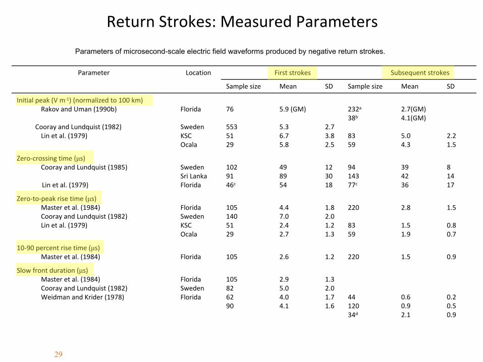