4.7 mechanism of littoral transport

4-103

4.7 Mechanism of Littoral Transport

4.7.1 Observation on Site Survey The coastal line in the study area is roughly divided into three parts based on topographic

characteristics: North Area from Khanom to Pak Phanang, Middle Area from Laem Talumphuk

of Nakhon Si Thammarat province to Pattani, and South Area from Laem Ta Chi of Pattani

province to Tak Bai at the southern extreme end of the study area (see Figure 4.7.1-1).

The results obtained about the mechanism of littoral drift in the study area is summarized as

follows: (North Area)

1. In the north part of the study area, Sichon to Tha Sala in Nakhon Si Thammarat province, the

predominant direction of littoral drift is southward.

2. Rate of littoral transport in this area is larger to the south.

3. Southern shoreline of Tha Sala channel is seriously eroded.

4. Southern limit of littoral transport in this area may be at Ban Sa Bua (2) village in Tha Sala

district.

5. Bottom materials in Pak Phanang Bay mainly composed of marine mud and, offshore area

from 17 km point along the Pak Phanang channel, is sand.

(Middle Area)

6. In the coastal area from Laem Talumphuk in Nakhon Si Thammarat province to Laem Son

On in Songkhla province, the predominant direction of littoral drift is northward.

7. From Ban Na Kot to Ban Nam Sap area in Nakhon Si Thammarat province erosion is taking

place.

8. In the middle part of the study area, Songkhla to Pattani, the predominant direction of littoral

drift is northward.

9. Rate of littoral transport in this area is a comparatively large amount.

10. Eroded areas in this area are situated in the northwest or west side of existing jetties, such as

Na Thap, Sakom, Thepha in Songkhla province and Bang Ra Pha, Tanyong Pao in Pattani

province.

11. Shoreline of Bang Ta Wa area in Pattani province is also seriously eroded even though no

jetty has been constructed.

12. Eastern limit of littoral transport in this area is at the most eastern groin in Bang Ta Wa near

the irrigation canal of the west of Ru Sa Mi Lae in Muan Pattani district.

13. Bottom materials in Pattani Bay are mainly composed of marine mud.

4-105

(South Area)

14. In the coastal area from Laem Ta Chi in Pattani province to Tak Bai in Narathiwat province,

the predominant direction of littoral drift is northward.

15. Rate of littoral transport in this area is rather large.

16. Eroded areas in this area are also situated in the west or northwest side of existing jetties,

such as Panare, Sai Buri in Pattani province and Narathiwat in Narathiwat province.

17. Coastal area of Tak Bai district in Narathiwat province located at the boundary with

Malaysia is one of the areas of the heaviest littoral drift in the study area.

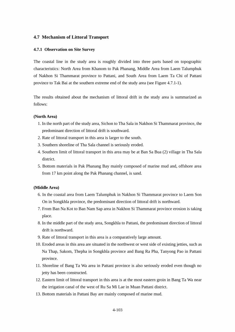
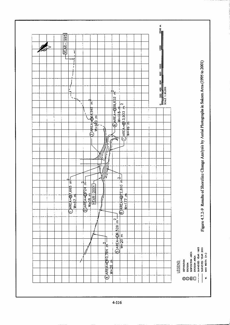
4.7.2 Analysis of Shoreline Changes by Aerial Photographs

Analysis of shoreline changes by using existing aerial photographs was carried out for

approximately 6 kilometers length along shorelines in Sichon, Tha Sala, Songkhla, Sakom and

Thepha areas.

Aerial photographs collected for the analysis are listed in Table 4.7.2-1.

Table 4.7.2-1 Aerial Photographs Collected for Analysis of Shoreline Changes

Area Latest Photograph

Date (Time) Previous Photographs

Date (Time) Construction

of Jetty Sichon February 2, 1995 (16h44m) April 28, 1975 (09h37m)

1997 – 1998

Tha Sala March 2, 1995 (16h39m) July 8, 1974 (10h05m) April 26, 1975 (09h37m)

1997 – 1998

Songkhla April 19, 1995 (08h00m) March 11, 1974 (11h13m) August 29, 1977 (15h29m)

1987 – 1992

Sakom April 9, 1995 (08h08m) April 28, 1973 (08h40m)

1998 – 1999

Thepha April 11, 1995 (09h09m) May 20, 1973 (09h47m) May 22, 1973 (09h59m)

1998 – 1999

Neither aerial photographs nor satellite images were available after jetties construction. Therefore,

field surveys for shoreline after jetties construction were carried out at every 500 meter intervals

along the shorelines in Sichon, Tha Sala, Songkhla, Sakom and Thepha areas in March 2001.

Results of the analysis of shoreline changes in each area are summarized in Tables 4.7.2-2 and

4.7.2-3, and shown in Figures 4.7.2-1 to 4.7.2-10.

4-106

Table 4.7.2-2 Results of Shoreline Change Analysis by Aerial Photographs

Coastal

Area

Area No. Deposition

Area (Max. Width) Erosion

Area (Max. Width) Remarks

No. 1 No. 2 No. 3 No. 4 No. 5 No. 6 No. 7 No. 8

227,881 m2 (140 m)

6,056 m2 (105 m) 17,635 m2 ( 53 m)

10,162 m2 ( 27 m)

21,632 m2 ( 53 m)

4,683 m2 ( 86 m)

2,053 m2 ( 35 m)

8,507 m2 ( 48 m)

Sum Net

283,367 m2

268,124 m2 15,243 m2

Sichon

Rate of Change

13,406 m2/year 2.23 m/year

1975 – 1995 (20 years)

Shoreline Length

6 km

No. 1 No. 2 No. 3 No. 4 No. 5 No. 6 No. 7

34,043 m2 ( 73 m)

10,285 m2 ( 40m)

8,818 m2 ( 23 m)

25,915 m2 ( 34 m) 4,211 m2 ( 14 m)

65,281 m2 ( 75 m) 38,374 m2 ( 42 m)

Sum Net

44,328 m2

142,599 m2

98,271 m2

Tha Sala

Rate of Change

4,680 m2/year 0.78 m/year

1974 – 1995 (21 years)

Shoreline Length

6 km

No. 1 No. 2 No. 3 No. 4 No. 5 No. 6 No. 7

341,609 m2 (189 m)

5,672 m2 ( 39m)

8,559 m2 ( 31 m)

69,377 m2 ( 92 m)

18,912 m2 ( 44 m)

19,849 m2 ( 29 m)

1,607 m2 ( 21 m)

Sum Net

425,217 m2

384,849 m2 40,368 m2

Songkhla

Rate of Change

18,326 m2/year 3.05 m/year

1974 – 1995 (21 years)

Shoreline Length

6 km

No. 1 No. 2 No. 3 No. 4 No. 5 No. 6 No. 7

81,388 m2 (120 m) 75,193 m2 (156 m)

205,820 m2 (320 m)

49,636 m2 ( 93 m)

161,242 m2 (123 m)

34,397 m2 ( 88 m) 7,212 m2 ( 35 m)

Sum Net

412,037 m2

209,186 m2 202,851 m2

Sakom

Rate of Change


1975 – 1995 (20 years)

Shoreline Length

6 km


197,288 m2 ( 88 m)

4,277 m2 ( 40 m)

17,714 m2 ( 50 m)

189,790 m2 (180 m)

42,838 m2 (100 m)

32,990 m2 ( 72 m) 23,852 m2 ( 23 m)

50,138 m2 (117 m)

Sum Net

409,069 m2

259,251 m2 149,818 m2

Thepha

Rate of Change

11,784 m2/year 1.96 m/year

1973 – 1995 (22 years)

Shoreline Length

6 km

4-107

Table 4.7.2-3 Results of Shoreline Change Analysis

Coastal

Area

Area No. Deposition

Area (Max. Width) Erosion

Area (Max. Width) Remarks

No. 1 No. 2 No. 3 No. 4 No. 5 No. 6 No. 7

21,272 m2 (124 m)

10,264 m2 ( 45 m) 3,156 m2 ( 20 m)

180,116 m2 (104 m)

11,001 m2 (121 m) 1,570 m2 ( 12 m)

812 m2 ( 17 m) Sum Net

34,692 m2

193,499 m2

158,807 m2

Sichon

Rate of Change

26,468 m2/year 6.62 m/year

1995 – 2001 (6 years)

Shoreline Length

4 km

No. 1 No. 2 No. 3 No. 4 No. 5 No. 6 No. 7

56,005 m2 ( 66 m)

37,135 m2 ( 80 m)

26,060 m2 ( 72 m)

6,395 m2 ( 15 m)

6,724 m2 ( 33 m) 19,804 m2 ( 85 m)

67,491 m2 ( 75 m)

Sum Net

119,200 m2

18,786 m2 100,414 m2

Tha Sala

Rate of Change


1995 – 2001 (6 years)

Shoreline Length

4.4 km

No. 1 No. 2

346,322 m2 (203 m)

63,092 m2 (119 m)

Sum Net

346,322 m2

283,230 m2 63,092 m2

Songkhla

Rate of Change

47,205 m2/year 11.80 m/year

1995 – 2001 (6 years)

Shoreline Length

4 km


7,665 m2 (57 m)

64,941 m2 (120 m)

72,810 m2 (177 m) 13,933 m2 ( 46 m)

724 m2 (18 m)

10,784 m2 (26 m) 9,528 m2 (20 m)

38,602 m2 (115 m) Sum Net

159,349 m2

99,711 m2 59,638 m2

Sakom

Rate of Change

16,619 m2/year 5.54 m/year

1995 – 2001 (6 years)

Shoreline Length

3 km

No. 1 No. 2 No. 3 No. 4 No. 5 No. 6

44,091 m2 ( 62 m)

368,644 m2 (500m)

2,744 m2 ( 38 m)

415 m2 ( 12 m)

12,083 m2 ( 82 m)

2,382 m2 ( 23 m)

Sum Net

415,479 m2

400,599 m2 14,880 m2

Thepha

Rate of Change

66,767 m2/year 11.13 m/year

1995 – 2001 (6 years)

Shoreline Length

6 km

4-118

4.7.3 Analysis of Shoreline Changes by N-Line Model

The analysis of shoreline changes using numerical methods was carried out to reproduce the

phenomena of littoral drift and to forecast the effect of littoral drift in the future in Sichon, Sakom

and Thepha areas.

The n-line model used for this study calculates longshore transport to each depth-line and

determines the amount of bathymetric changes in the area concerned.

1) Calculation of Waves

(a) Basic Equation

When the wave is irregular with direction spectrums, Karlsson has drawn an energy balance

equation as follows:

(Energy Conservation Equation)

0Q)DV( =−⋅∇+∂∂

(1)

Here,

θ∂

∂∂∂

∂∂

∂∂

=∇ ,f

,y

,x

(2)

D (x, y, f, θ, t) : energy density

V : speed of energy density

x, y : coordinates

f : frequency

θ : angle

Q : energy transfer

Follows will be obtained as an energy balance equation for an irregular wave, if refer to Q= 0 in

equation (2).

0)DV()DV(y

)DV(x yx =

θ∂∂

+∂∂

+∂∂

θ (3)

Here,

Ｖｘ＝Ｃｇcodθ ，ＤＶｙ＝Ｃｇsinθ

4-119

θ

∂∂

−θ∂∂

=θ cosyC

sinxC

CCg

V

Cg : group velocity , C : wave velocity.

Directional spectrum of irregular wave is expressed as a product of frequency spectrum and

direction function as follows;

Ｄ（ｆ，θ）＝Ｓ（ｆ）Ｇ（ｆ，θ） (4)

Here,

Ｄ（ｆ，θ）： directional spectrum

Ｓ（ｆ）： frequency spectrum

Ｇ（ｆ，θ）： directional function

Frequency spectrum expresses the distribution of energy density to frequency and can be obtained

by integrating direction spectrum.

2/n

2n)f(S −∫= Ｄ（ｆ，θ）ｄθ (5)

The distributed type of this frequency spectrum is standardized as follows;

Ｓ（ｆ）＝ａｆ-5 exp（-bf -4） (6)

(Bretschneider type)

44

2

T0288.1

b,TH

2572.0a == (7)

H and T : significant wave height and its period

Direction function expresses the distribution by the direction of energy density, and

Bretschneider’s function is shown as follows:

2cos)S('G),f(G S2

1

∂=θ (8)

Here,

1

S2maxmax

'1 d

2cos)S(G

−

θθ−

θ

∂

∫= (9)

G1' (S) is a standardization function for satisfying the lower equation which is a general definition

of directional function.

1d),f(Gnn =θθ∫ −

4-120

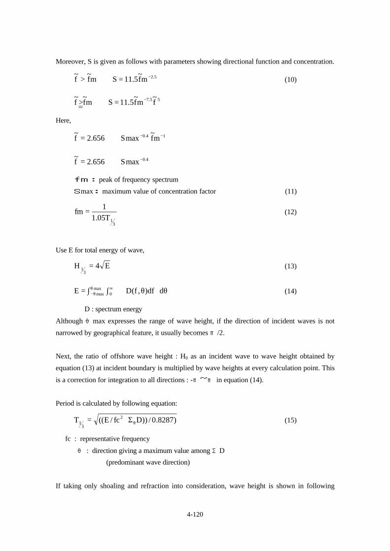
Moreover, S is given as follows with parameters showing directional function and concentration.

5.2mf~

5.11Smf~

f~ −=> (10)

55.7 f~

mf~

5.11Smf~

f~ −=>

Here,

14.0 mf~

maxS656.2f~ −−=

4.0maxS656.2f~ −=

ｆｍ： peak of frequency spectrum

Ｓmax： maximum value of concentration factor (11)

31T05.1

1fm = (12)

Use E for total energy of wave,

E4H3

1 = (13)

θ⋅θ∫∫= ∞θθ− ddf),f(DE 0max

max (14)

D : spectrum energy

Although θmax expresses the range of wave height, if the direction of incident waves is not

narrowed by geographical feature, it usually becomes π/2.

Next, the ratio of offshore wave height : H0 as an incident wave to wave height obtained by

equation (13) at incident boundary is multiplied by wave heights at every calculation point. This

is a correction for integration to all directions : -π～π in equation (14).

Period is calculated by following equation:

)8287.0/))Dfc/E((T 2

31 θΣ⋅= (15)

fc : representative frequency

θ : direction giving a maximum value among ΣD

(predominant wave direction)

If taking only shoaling and refraction into consideration, wave height is shown in following

4-121

equation:

Ｈ1/3＝ＫsiＨ0’ ：ｈ／Ｌ0≧0.2

＝min((β0Ｈ0’＋β1h)，βmaxＨ0’，ＫsＨ0’) ：ｈ／Ｌ0＜0.2 (16)

Here,

Ｈ0’=Ｈs※／Ｋsi

min( )： minimum value within ( )

H0' ： significant wave height

Ks ： shallow wave factor

Ksi ： shallow wave factor of small amplitude waves

Hs※ ： significant wave height, taking only shoaling and refraction into consideration

Shallow wave factor in equation (16) was calculated basing on nonlinear modification theory of

Sudo,

β0＝0.028（Ｈ0’／Ｌ0）-0.38 exp（20tan1.5θ）

β1＝0.52 exp（4.2tanθ）

βmax＝max（0.92，0.32（Ｈ0’／Ｌ0）-0.29 exp（2.4tanθ）） (17)

Here,

L0 ： wave length of offshore wave

tanθ ： bottom slope

(b) Calculation Conditions

The conditions used for calculation of wave refraction are as shown below.

① Wave Direction

Using the frequency distribution of winds in the northeast monsoon season : November to January

during 1980–2001, wave directions were decided as the highest frequency of N－E－S direction,

which is a direction from the sea side.

The most predominant wind directions at each station in and near the study area are shown in

Table 4.7.3-1.

4-122

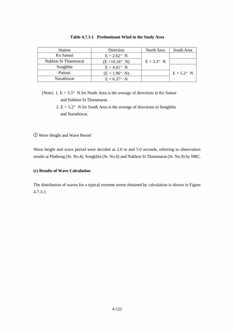
Table 4.7.3-1 Predominant Wind in the Study Area

Station Direction North Area South Area

Ko Samui E + 2.62°N Nakhon Si Thammarat (E +10.34°N) E + 3.3°N

Songkhla E + 4.01°N Pattani (E + 1.96°N) E + 5.2°N

Narathiwat E + 6.37°N

(Note) 1. E + 3.3°N for North Area is the average of directions in Ko Samui

and Nakhon Si Thammarat.

2. E + 5.2°N for South Area is the average of directions in Songkhla

and Narathiwat.

② Wave Height and Wave Period

Wave height and wave period were decided as 2.0 m and 5.0 seconds, referring to observation

results at Plathong (St. No.4), Songkhla (St. No.6) and Nakhon Si Thammarat (St. No.9) by NRC.

(c) Results of Wave Calculation

The distribution of waves for a typical extreme storm obtained by calculation is shown in Figure

4.7.3-1.

4-123

Figure 4.7.3-1 Wave Refraction Map in the Study Area

(offshore wave direction : E +3.3°& E +5.2°)

H0 = 2.0 m, T0 = 5.0 sec

Tak Bai

NARATHIWAT

PATTANI

SONGKHLA

650 700 750 800 850

700

750

800

850

Fig.

Wave Refraction Map(offshore wave direction : E+3.3-5.2)

H0=2m,T0=5s

PATTANI

SONGKHLA

SATHING RHRA

RANOT

HUA SAI

PAK PHANANG

THA SALA

SICHON

KHANOM

600 650 700 750 800

800

850

900

950

1000

1050

E+3.3°

E+5.2°

4-124

2) Analysis of Shoreline Changes

(a) Basic Equation of N-Line Model

① Basic Equation of Longshore Littoral Transport

The n-line model calculates longshore littoral transport to each depth-line and determines the

amount of bathymetric changes.

The longshore littoral transport rate : Q will be given by equation (1)

bb0

bbb2

b

cossinF

cossin)Cg(gH8f

Q

αα=

ααρ= (1)

Here,

ｆ： littoral transport factor

ρ ： seawater density

ｇ： gravity

Ｈb： breaking wave height

αb： breaking wave direction

(Cg)b： group velocity of breaker wave point

X-axis is taken in the direction of coast, and y-axis is taken in the direction of right-angle on

x-axis. When we assume that αb is fully small, equation (2) will be:

)yx

(tanFQ b0 ∂∂

−α= (2)

This equation is adapted for the area divided into “n” contours. Equation (3) can be gotten, we use

qk for littoral transport rate of the depth to k = 1,…, n and suppose that the same relation as

equation (2) is adapted between the distance among contour lines : yk and qk.

)xy

(tankFq k00k ∂

∂−α= (3)

Here,

Ｆ0k＝Ｆ0μk , Σμk＝1.

μk is a comparison constant which gives littoral transport for each water depth and is calculated

using equation (4) by giving a vertical distribution of longshore littoral transport rate :ξ(z).

dz)z(/dz)z(hr

hc

1zk

zkk ∫∫ ξξ=µ+

(4)

4-125

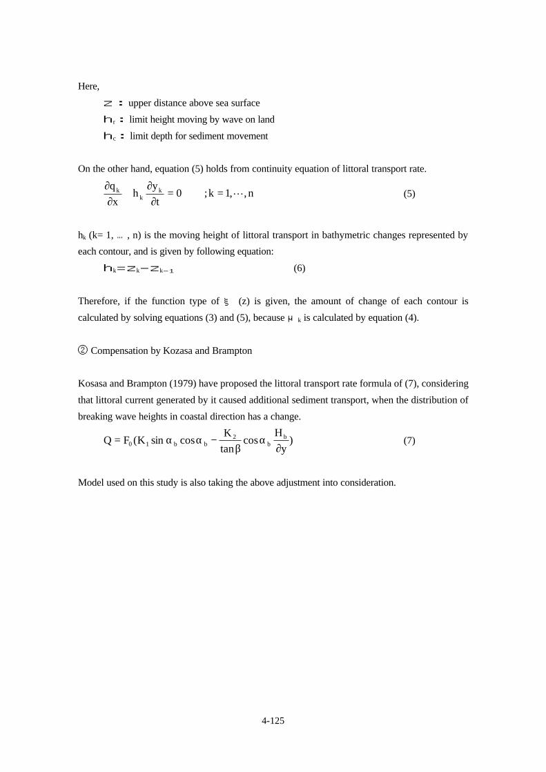
Here,

ｚ： upper distance above sea surface

ｈr ： limit height moving by wave on land

ｈc ： limit depth for sediment movement

On the other hand, equation (5) holds from continuity equation of littoral transport rate.

n,,1k;0t

yh

xq k

kk L==

∂∂

+∂

∂ (5)

hk (k= 1, …, n) is the moving height of littoral transport in bathymetric changes represented by

each contour, and is given by following equation:

ｈk＝ｚk－ｚk－１ (6)

Therefore, if the function type of ξ (z) is given, the amount of change of each contour is

calculated by solving equations (3) and (5), because μk is calculated by equation (4).

② Compensation by Kozasa and Brampton

Kosasa and Brampton (1979) have proposed the littoral transport rate formula of (7), considering

that littoral current generated by it caused additional sediment transport, when the distribution of

breaking wave heights in coastal direction has a change.

)y

Hcos

tanK

cossinK(FQ bb

2bb10 ∂

αβ

−αα= (7)

Model used on this study is also taking the above adjustment into consideration.

4-126

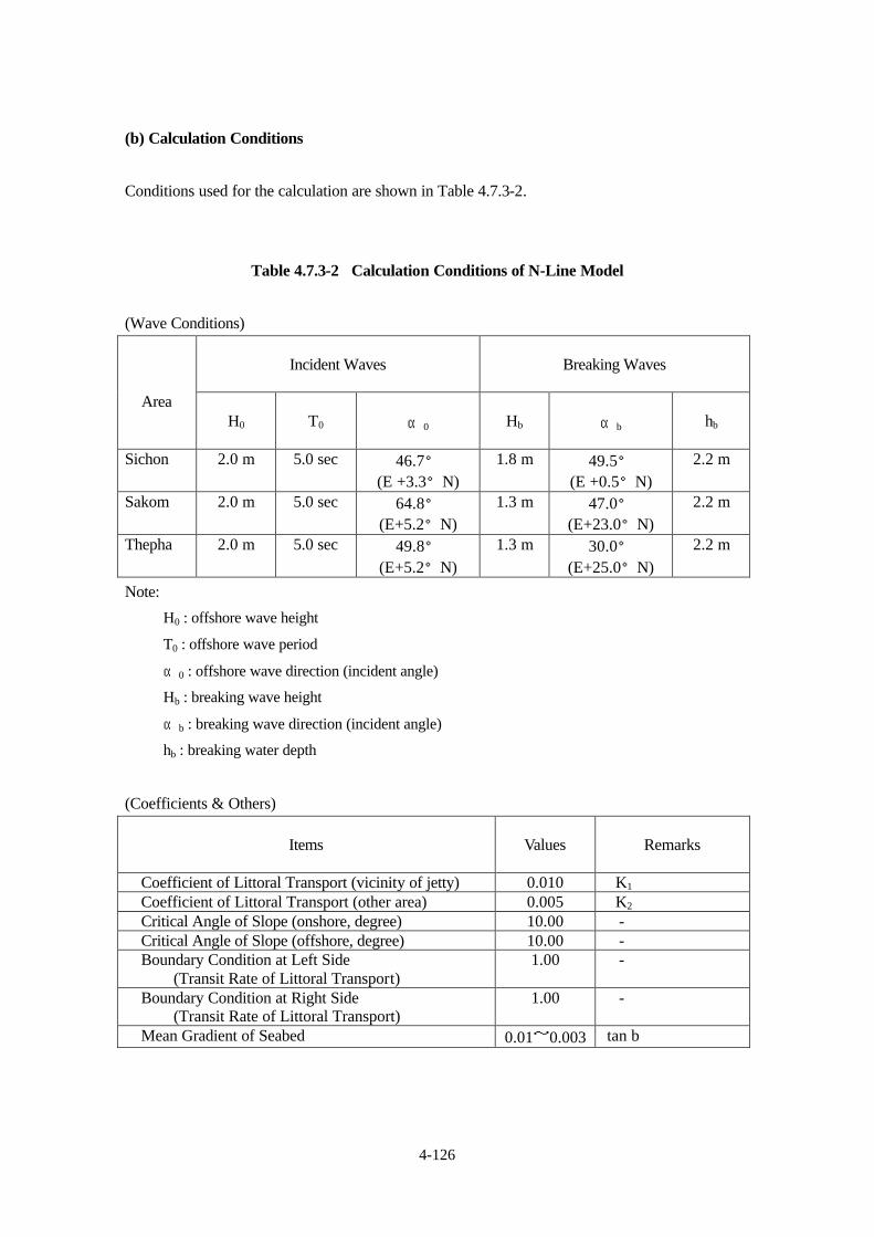
(b) Calculation Conditions

Conditions used for the calculation are shown in Table 4.7.3-2.

Table 4.7.3-2 Calculation Conditions of N-Line Model

(Wave Conditions)

Incident Waves

Breaking Waves

Area H0

T0

α0

Hb

αb

hb

Sichon 2.0 m 5.0 sec 46.7° (E +3.3°N)

1.8 m 49.5° (E +0.5°N)

2.2 m

Sakom 2.0 m 5.0 sec 64.8° (E+5.2°N)

1.3 m 47.0° (E+23.0°N)

2.2 m

Thepha 2.0 m 5.0 sec 49.8° (E+5.2°N)

1.3 m 30.0° (E+25.0°N)

2.2 m

Note:

H0 : offshore wave height

T0 : offshore wave period

α0 : offshore wave direction (incident angle)

Hb : breaking wave height

αb : breaking wave direction (incident angle)

hb : breaking water depth

(Coefficients & Others)

Items

Values

Remarks

Coefficient of Littoral Transport (vicinity of jetty) 0.010 K1 Coefficient of Littoral Transport (other area) 0.005 K2 Critical Angle of Slope (onshore, degree) 10.00 - Critical Angle of Slope (offshore, degree) 10.00 - Boundary Condition at Left Side

(Transit Rate of Littoral Transport) 1.00 -

Boundary Condition at Right Side (Transit Rate of Littoral Transport)

1.00 -

Mean Gradient of Seabed 0.01～0.003 tan b

4-127

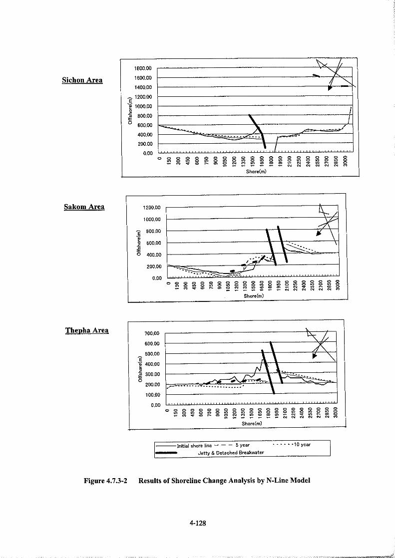
(c) Calculation Results

Shoreline changes after five and ten years forecast by n-line model are shown in Figure 4.7.3-2.

The initial shoreline in this figure means the state in 2001 and the shoreline means zero meter of

chart datum level.

Results show that the shoreline in the future will not change so much except in the vicinity of the

left side jetty in Sichon area.

In Sakom area, the deposition will increase on the right side of the jetties. On the left side of the

jetties, detached breakwaters show an effect and a large erosion area will appear after the detached

breakwaters.

The shoreline change in Thepha area is almost the same as that in Sakom area.

Rates of littoral transport in Sichon, Sakom and Thepha areas calculated by n-line model are

shown in Figure 4.7.3-3.

The amount of deposition and/or erosion at every calculation point, which is the difference of

littoral transport rates between adjoining points, is also shown in Figure 4.7.3-4.

Rates of littoral transport were calculated as about 2.5 x 104 m3/year, 1.1 x 105 m3/year and 1.0 x

105 m3/year in Sichon, Sakom and Thepha areas, respectively.

4.7 mechanism of littoral transport

Documents