448-2013: estimating censored price elasticities … 448-2013 estimating censored price elasticities...

Paper 448-2013

Estimating Censored Price Elasticities Using SAS/ETS®: Frequentistand Bayesian Approaches

Christian Macaro, Jan Chvosta, Kenneth Sanford, James LemieuxSAS Institute Inc.

ABSTRACT

The number of rooms rented by a hotel, spending by “loyalty card” customers, automobile purchases byhouseholds—these are just a few examples of variables that can best be described as “limited” variables.When limited (censored or truncated) variables are chosen as dependent variables, certain necessaryassumptions of linear regression are violated. This paper discusses the use of SAS/ETS® tools to analyzedata in which the dependent variable is limited. It presents several examples that use the classical approachand the Bayesian approach that was recently added to the QLIM procedure, emphasizing the advantagesand disadvantages that each approach provides.

INTRODUCTION

Economic theory suggests that as the price of a product or service rises, the demand for it falls, if all otherfactors are equal. This theory is often applied in the field of revenue management. As part of a company’soptimization strategy, revenue management analysts are often asked to build models that allow prices toinfluence the number of units sold and therefore affect the company’s revenue. A necessary componentof this effort is the development of price elasticities. Price elasticity measures how quantities respond tochanges in price. The analyst usually uses a data set that contains past prices and quantities, along withadditional explanatory variables, and applies regression techniques to estimate this historical relationship.Price elasticities are used in many revenue management applications. Sophisticated revenue managementsystems for clothing retailers, hotels, and airline and sports ticket agencies incorporate price elasticities intotheir optimization routines. Analysts must give special consideration to the statistical or, more precisely, theeconometric methods that they use to estimate these elasticities. Neglecting certain aspects of the data andthe model can severely bias the elasticity estimate and lead to nonoptimal policy recommendations. Amongthe important considerations is awareness of the possible values that the data might realize.

This paper focuses on hotel data. The maximum number of hotel rooms that can be occupied on a given dayis limited by the capacity of the hotel. This capacity is fixed over any reasonable period of time. Therefore,the maximum number of rooms that can be booked for any given day must be less than or equal to thecapacity of the hotel. This type of data is commonly referred to as censored data (Maddala 1983). In thecase of censored data, analysts must use special considerations to estimate price elasticities.

This paper presents a classic case of censoring and the econometric concerns that arise from ignoringcensoring. It then presents a real-life example of censoring in the hotel industry. Finally, the paper shows howto estimate the model by using the newest Bayesian estimation techniques that are available in SAS/ETS12.1.

ELASTICITY ESTIMATION

Suppose a management analyst is charged with estimating the price elasticity �p for a product or service.More formally, the price elasticity of demand is

�pD�Quantity.Price/=Quantity.Price/

�Price=Price

where Quantity(Price) is the dependent variable in the regression of quantity on price of the product andPrice is the price of the product. Based on this regression model, ordinary least squares (OLS) or some other

1

Statistics and Data AnalysisSAS Global Forum 2013

method of estimation can provide consistent estimates of the price elasticity if the error in the regression isnot correlated with included regressors and if the dependent variable is not censored. The problem for ahotelier (or for any analyst in a capacity-constrained industry) is far more complex. Specifically, the hotelieris limited by the number of rooms available. Therefore, the upper bound on the number of rooms violatesthe assumption of normality of the data and the assumptions of the classic normal regression model. Thisproblem of a censored distribution is relatively minor when the data rarely reach the threshold. However, forgoods whose capacity is highly constrained, such as tickets and hotel rooms, sellouts are fairly common.In these cases, the upper-censoring problem creates meaningful challenges for estimating the elasticity ofdemand.

This paper examines two upper-censoring cases. The first example simulates a typical censored regressionproblem with a fixed threshold, such that the bias in the elasticity is negative and causes the value of theelasticity to be smaller in absolute value than is accurate. This leads the analyst to conclude that consumersare less price sensitive than they have actually demonstrated themselves to be, which, in turn, leads to ahigher-than-optimal price being set. In the second example, a real data set is analyzed. These data arecharacterized by a non-fixed upper censoring that causes a positive bias in the elasticity estimation. Thisleads the analyst to conclude that consumers are more price sensitive than they have actually demonstratedthemselves to be. This result might suggest setting a lower-than-optimal price.

BIAS DUE TO CENSORING: A SIMULATED EXAMPLE

Econometric problems that are associated with the classic case of right censoring are prevalent in theliterature (Maddala 1983). To illustrate the bias that is associated with ignoring upper censoring, this examplegenerates data that have a coefficient on the price variable of –0.5 and have errors distributed normally. Itestimates price elasticities under two scenarios: OLS on the uncensored data and OLS on the censoreddata. Figure 1 shows the price elasticities of the two estimates. A large bias is associated with ignoring thecensoring. The magnitude of the bias in this case is approximately 30% in the downward direction. This isthe typical effect on the magnitude of the estimates that are affected by right censoring. Figure 1 graphicallypresents the magnitude of the bias.

2


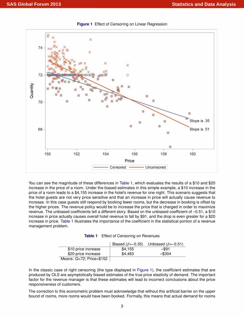
Figure 1 Effect of Censoring on Linear Regression

You can see the magnitude of these differences in Table 1, which evaluates the results of a $10 and $20increase in the price of a room. Under the biased estimates in this simple example, a $10 increase in theprice of a room leads to a $4,155 increase in the hotel’s revenue for one night. This scenario suggests thatthe hotel guests are not very price sensitive and that an increase in price will actually cause revenue toincrease. In this case guests still respond by booking fewer rooms, but the decrease in booking is offset bythe higher prices. The revenue policy would be to increase the price that is charged in order to maximizerevenue. The unbiased coefficients tell a different story. Based on the unbiased coefficient of –0.51, a $10increase in price actually causes overall hotel revenue to fall by $91, and the drop is even greater for a $20increase in price. Table 1 illustrates the importance of the coefficient in the statistical portion of a revenuemanagement problem.

Table 1 Effect of Censoring on Revenues

Biased (ˇ=–0.35) Unbiased (ˇ=–0.51)$10 price increase $4,155 –$91$20 price increase $4,483 –$304

Means: Q=72; Price=$152

In the classic case of right censoring (the type displayed in Figure 1), the coefficient estimates that areproduced by OLS are asymptotically biased estimates of the true price elasticity of demand. The importantfactor for the revenue manager is that these estimates will lead to incorrect conclusions about the priceresponsiveness of customers.

The correction to this econometric problem must acknowledge that without this artificial barrier on the upperbound of rooms, more rooms would have been booked. Formally, this means that actual demand for rooms

3


(Quantity) is observed when room occupancy is below capacity, but as the demand exceeds the upperbound (C �, a constant), only C � is observed instead of the true demand for the rooms. Econometrically, thisamounts to maximizing a modified log-likelihood function that takes censoring into consideration.

The next section shows the implications of ignoring censoring by using a more realistic example in the hotelindustry. It demonstrates how censoring might actually occur in practice and how accurately estimating priceresponsiveness leads to more accurate pricing recommendations.

BIAS DUE TO CENSORING: A REAL-DATA EXAMPLE

The following data were collected for four different hotel properties (A, B, C, D) over a period of one year:

• price of booking

• occupancy (the number of booked rooms)

• occupancy rate (the overall occupancy percentage of the hotel)

• date when occupancy occurred

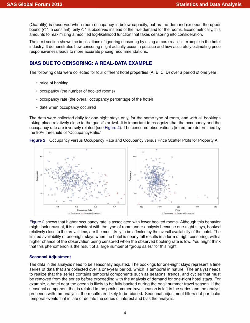
The data were collected daily for one-night stays only, for the same type of room, and with all bookingstaking place relatively close to the guest’s arrival. It is important to recognize that the occupancy and theoccupancy rate are inversely related (see Figure 2). The censored observations (in red) are determined bythe 90% threshold of “OccupancyRatio.”

Figure 2 Occupancy versus Occupancy Rate and Occupancy versus Price Scatter Plots for Property A

Figure 2 shows that higher occupancy rate is associated with fewer booked rooms. Although this behaviormight look unusual, it is consistent with the type of room under analysis because one-night stays, bookedrelatively close to the arrival time, are the most likely to be affected by the overall availability of the hotel. Thelimited availability of one-night stays when the hotel is nearly full results in a form of right censoring, with ahigher chance of the observation being censored when the observed booking rate is low. You might thinkthat this phenomenon is the result of a large number of "group sales" for this night.

Seasonal Adjustment

The data in the analysis need to be seasonally adjusted. The bookings for one-night stays represent a timeseries of data that are collected over a one-year period, which is temporal in nature. The analyst needsto realize that the series contains temporal components such as seasons, trends, and cycles that mustbe removed from the series before proceeding with the analysis of demand for one-night hotel stays. Forexample, a hotel near the ocean is likely to be fully booked during the peak summer travel season. If theseasonal component that is related to the peak summer travel season is left in the series and the analystproceeds with the analysis, the results are likely to be biased. Seasonal adjustment filters out particulartemporal events that inflate or deflate the series of interest and bias the analysis.

4


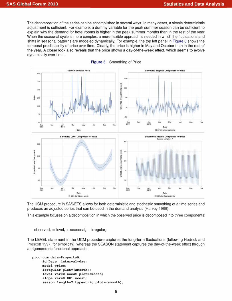
The decomposition of the series can be accomplished in several ways. In many cases, a simple deterministicadjustment is sufficient. For example, a dummy variable for the peak summer season can be sufficient toexplain why the demand for hotel rooms is higher in the peak summer months than in the rest of the year.When the seasonal cycle is more complex, a more flexible approach is needed in which the fluctuations andshifts in seasonal patterns are modeled dynamically. For example, the top left panel in Figure 3 shows thetemporal predictability of price over time. Clearly, the price is higher in May and October than in the rest ofthe year. A closer look also reveals that the price shows a day-of-the-week effect, which seems to evolvedynamically over time.

Figure 3 Smoothing of Price

The UCM procedure in SAS/ETS allows for both deterministic and stochastic smoothing of a time series andproduces an adjusted series that can be used in the demand analysis (Harvey 1989).

This example focuses on a decomposition in which the observed price is decomposed into three components:

observedt D levelt C seasonalt C irregulart

The LEVEL statement in the UCM procedure captures the long-term fluctuations (following Hodrick andPrescott 1997, for simplicity), whereas the SEASON statement captures the day-of-the-week effect througha trigonometric functional approach:

proc ucm data=PropertyA;id Date interval=day;model price;irregular plot=(smooth);level var=0 noest plot=smooth;slope var=0.001 noest;season length=7 type=trig plot=(smooth);

5


run;

Figure 3 shows the estimates of the three unobserved components. Notice that the irregular componentis centered around 0, whereas the level component retains the original magnitude of the series. Forinterpretational purposes, you can shift the irregular component back to the original magnitude of the seriesby adding a term that represents the mean of the series.

Ordinary Least Squares and Censored Linear Regression Analysis

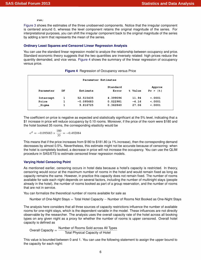
You can use the standard linear regression model to analyze the relationship between occupancy and price.Standard economic theory suggests that the two quantities are inversely related: high prices reduce thequantity demanded, and vice versa. Figure 4 shows the summary of the linear regression of occupancyversus price.

Figure 4 Regression of Occupancy versus Price

Parameter Estimates

Standard ApproxParameter DF Estimate Error t Value Pr > |t|

Intercept 1 52.515435 4.399096 11.94 <.0001Price 1 -0.095683 0.022981 -4.16 <.0001_Sigma 1 9.816725 0.362840 27.06 <.0001

The coefficient on price is negative as expected and statistically significant at the 5% level, indicating that a$1 increase in price will reduce occupancy by 0.10 rooms. Moreover, if the price of the room were $180 andthe hotel booked 35 rooms, the corresponding elasticity would be

�pD �0:095683 �

180

35D �0:492084

This means that if the price increases from $180 to $181.80 (a 1% increase), then the corresponding demanddecreases by almost 0.5%. Nevertheless, this estimate might not be accurate because of censoring: whenthe hotel is completely booked, a decrease in price will not increase the occupancy. You can use the QLIMprocedure in SAS/ETS to estimate censored linear regression models.

Varying Hotel Censoring Point

As mentioned earlier, censoring occurs in hotel data because a hotel’s capacity is restricted. In theory,censoring would occur at the maximum number of rooms in the hotel and would remain fixed as long ascapacity remains the same. However, in practice this capacity does not remain fixed. The number of roomsavailable for sale each night depends on several factors, including the number of multinight stays (peoplealready in the hotel), the number of rooms booked as part of a group reservation, and the number of roomsthat are not in service.

You can formalize the theoretical number of rooms available for sale as

Number of One-Night Stays D Total Hotel Capacity � Number of Rooms Not Booked as One-Night Stays

The analysis here considers that all three sources of capacity restrictions influence the number of availablerooms for one-night stays, which is the dependent variable in the model. These influences are not directlyobservable by the researcher. The analysis uses the overall capacity rate of the hotel across all bookingtypes on any given night as a proxy for whether the number of rooms is upper censored. Overall hotelcapacity is defined as

Overall Capacity DNumber of Rooms Sold across All Types

Total Physical Capacity of Hotel

This value is bounded between 0 and 1. You can use the following statement to assign the upper bound tothe capacity for each night:

6


proc qlim data=PropertyA;model Occupancy = Price / censored(lb=0 ub=up);run;

The CENSORED option enables you to introduce an upper-censoring series (“up”) to detect which data wereobserved at a full occupancy rate. The CENSORED option also enables you to set a physical lower bound at0: demand cannot be negative.

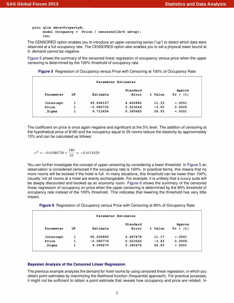
Figure 5 shows the summary of the censored linear regression of occupancy versus price when the uppercensoring is determined by the 100% threshold of occupancy rate.

Figure 5 Regression of Occupancy versus Price with Censoring at 100% of Occupancy Rate

Parameter Estimates


Intercept 1 49.896157 4.402882 11.33 <.0001Price 1 -0.080730 0.023046 -3.50 0.0005_Sigma 1 9.712454 0.360665 26.93 <.0001

The coefficient on price is once again negative and significant at the 5% level. The addition of censoring atthe hypothetical price of $180 and the occupancy equal to 35 rooms reduce the elasticity by approximately15% and can be calculated as follows:

�pD �0:0:080730 �

180

35D �0:4151829

You can further investigate the concept of upper censoring by considering a lower threshold. In Figure 5 anobservation is considered censored if the occupancy rate is 100%. In practical terms, this means that nomore rooms will be booked if the hotel is full. In many situations, this threshold can be lower than 100%.Usually, not all rooms at a hotel are evenly exchangeable. For example, it is unlikely that a luxury suite willbe deeply discounted and booked as an economy room. Figure 6 shows the summary of the censoredlinear regression of occupancy on price when the upper censoring is determined by the 90% threshold ofoccupancy rate instead of the 100% threshold. This indicates that lowering the threshold has very littleimpact.

Figure 6 Regression of Occupancy versus Price with Censoring at 90% of Occupancy Rate

Parameter Estimates


Intercept 1 50.230885 4.497878 11.17 <.0001Price 1 -0.080776 0.023562 -3.43 0.0006_Sigma 1 9.599270 0.360472 26.63 <.0001

Bayesian Analysis of the Censored Linear Regression

The previous example analyzes the demand for hotel rooms by using censored linear regression, in which youobtain point estimates by maximizing the likelihood function (frequentist approach). For practical purposes,it might not be sufficient to obtain a point estimate that reveals how occupancy and price are related. In

7


many situations, assessing the uncertainty can be just as important. From a hotel revenue managementperspective, questions such as the following are very important:

• What is the probability that the hotel will be completely booked at a given price per room?

• What is the price that will predict a sold-out hotel with 70% probability?

• What is the probability that the occupancy will remain the same if the price is increased by 5%?

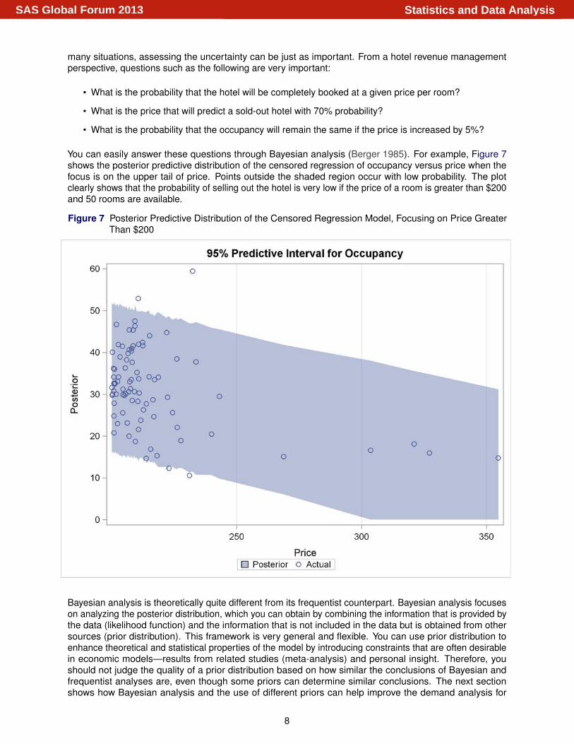
You can easily answer these questions through Bayesian analysis (Berger 1985). For example, Figure 7shows the posterior predictive distribution of the censored regression of occupancy versus price when thefocus is on the upper tail of price. Points outside the shaded region occur with low probability. The plotclearly shows that the probability of selling out the hotel is very low if the price of a room is greater than $200and 50 rooms are available.

Figure 7 Posterior Predictive Distribution of the Censored Regression Model, Focusing on Price GreaterThan $200

Bayesian analysis is theoretically quite different from its frequentist counterpart. Bayesian analysis focuseson analyzing the posterior distribution, which you can obtain by combining the information that is provided bythe data (likelihood function) and the information that is not included in the data but is obtained from othersources (prior distribution). This framework is very general and flexible. You can use prior distribution toenhance theoretical and statistical properties of the model by introducing constraints that are often desirablein economic models—results from related studies (meta-analysis) and personal insight. Therefore, youshould not judge the quality of a prior distribution based on how similar the conclusions of Bayesian andfrequentist analyses are, even though some priors can determine similar conclusions. The next sectionshows how Bayesian analysis and the use of different priors can help improve the demand analysis for

8


one-night hotel stays in which you observe a limited history for one property.

Analysis of Property B with Several Priors

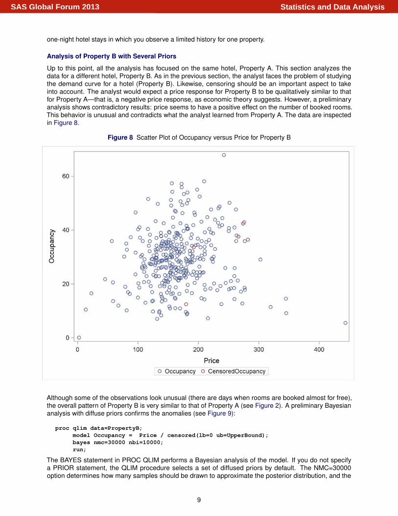
Up to this point, all the analysis has focused on the same hotel, Property A. This section analyzes thedata for a different hotel, Property B. As in the previous section, the analyst faces the problem of studyingthe demand curve for a hotel (Property B). Likewise, censoring should be an important aspect to takeinto account. The analyst would expect a price response for Property B to be qualitatively similar to thatfor Property A—that is, a negative price response, as economic theory suggests. However, a preliminaryanalysis shows contradictory results: price seems to have a positive effect on the number of booked rooms.This behavior is unusual and contradicts what the analyst learned from Property A. The data are inspectedin Figure 8.

Figure 8 Scatter Plot of Occupancy versus Price for Property B

Although some of the observations look unusual (there are days when rooms are booked almost for free),the overall pattern of Property B is very similar to that of Property A (see Figure 2). A preliminary Bayesiananalysis with diffuse priors confirms the anomalies (see Figure 9):

proc qlim data=PropertyB;model Occupancy = Price / censored(lb=0 ub=UpperBound);bayes nmc=30000 nbi=10000;run;

The BAYES statement in PROC QLIM performs a Bayesian analysis of the model. If you do not specifya PRIOR statement, the QLIM procedure selects a set of diffused priors by default. The NMC=30000option determines how many samples should be drawn to approximate the posterior distribution, and the

9


NBI=10000 option specifies how long the burn-in period should be (how many initial samples to discard sothat the posterior distribution can be approximated well).

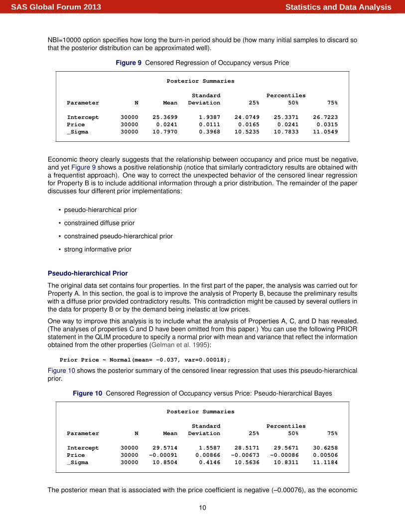
Figure 9 Censored Regression of Occupancy versus Price

Posterior Summaries

Standard PercentilesParameter N Mean Deviation 25% 50% 75%

Intercept 30000 25.3699 1.9387 24.0749 25.3371 26.7223Price 30000 0.0241 0.0111 0.0165 0.0241 0.0315_Sigma 30000 10.7970 0.3968 10.5235 10.7833 11.0549

Economic theory clearly suggests that the relationship between occupancy and price must be negative,and yet Figure 9 shows a positive relationship (notice that similarly contradictory results are obtained witha frequentist approach). One way to correct the unexpected behavior of the censored linear regressionfor Property B is to include additional information through a prior distribution. The remainder of the paperdiscusses four different prior implementations:

• pseudo-hierarchical prior

• constrained diffuse prior

• constrained pseudo-hierarchical prior

• strong informative prior

Pseudo-hierarchical Prior

The original data set contains four properties. In the first part of the paper, the analysis was carried out forProperty A. In this section, the goal is to improve the analysis of Property B, because the preliminary resultswith a diffuse prior provided contradictory results. This contradiction might be caused by several outliers inthe data for property B or by the demand being inelastic at low prices.

One way to improve this analysis is to include what the analysis of Properties A, C, and D has revealed.(The analyses of properties C and D have been omitted from this paper.) You can use the following PRIORstatement in the QLIM procedure to specify a normal prior with mean and variance that reflect the informationobtained from the other properties (Gelman et al. 1995):

Prior Price ~ Normal(mean= -0.037, var=0.00018);

Figure 10 shows the posterior summary of the censored linear regression that uses this pseudo-hierarchicalprior.

Figure 10 Censored Regression of Occupancy versus Price: Pseudo-hierarchical Bayes

Posterior Summaries

Standard PercentilesParameter N Mean Deviation 25% 50% 75%

Intercept 30000 29.5714 1.5587 28.5171 29.5671 30.6258Price 30000 -0.00091 0.00866 -0.00673 -0.00086 0.00506_Sigma 30000 10.8504 0.4146 10.5636 10.8311 11.1184

The posterior mean that is associated with the price coefficient is negative (–0.00076), as the economic

10


theory suggests. This improvement is the result of introducing information from the analysis of Properties A,C, and D. The idea of introducing extra-experimental information through a prior distribution is essential forBayesian analysis and, in many cases, can correct for anomalies in the data.

Constrained Diffuse Prior

Another way to ensure a negative posterior mean of the regression coefficient that is associated with price isto assume a uniform prior with an upper bound set at 0. This approach is justified by standard economictheory: demand is inversely related to price. You can use the following PRIOR statement in PROC QLIM toset such a prior distribution:

Prior Price ~ Uniform(max=0);

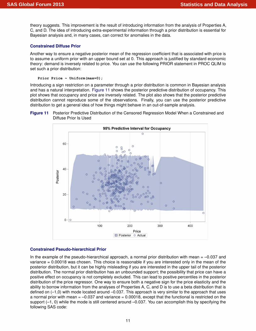
Introducing a sign restriction on a parameter through a prior distribution is common in Bayesian analysisand has a natural interpretation. Figure 11 shows the posterior predictive distribution of occupancy. Thisplot shows that occupancy and price are inversely related. The plot also shows that the posterior predictivedistribution cannot reproduce some of the observations. Finally, you can use the posterior predictivedistribution to get a general idea of how things might behave in an out-of-sample analysis.

Figure 11 Posterior Predictive Distribution of the Censored Regression Model When a Constrained andDiffuse Prior Is Used

Constrained Pseudo-hierarchical Prior

In the example of the pseudo-hierarchical approach, a normal prior distribution with mean = –0.037 andvariance = 0.00018 was chosen. This choice is reasonable if you are interested only in the mean of theposterior distribution, but it can be highly misleading if you are interested in the upper tail of the posteriordistribution. The normal prior distribution has an unbounded support; the possibility that price can have apositive effect on occupancy is not completely excluded. This can lead to positive percentiles in the posteriordistribution of the price regressor. One way to ensure both a negative sign for the price elasticity and theability to borrow information from the analyses of Properties A, C, and D is to use a beta distribution that isdefined on (–1,0) with mode located around –0.037. This approach is very similar to the approach that usesa normal prior with mean = –0.037 and variance = 0.00018, except that the functional is restricted on thesupport (–1, 0) while the mode is still centered around –0.037. You can accomplish this by specifying thefollowing SAS code:

11


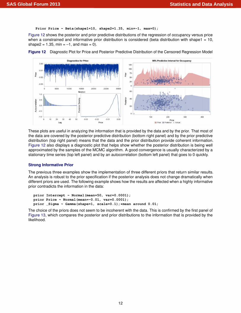
Prior Price ~ Beta(shape1=10, shape2=1.35, min=-1, max=0);

Figure 12 shows the posterior and prior predictive distributions of the regression of occupancy versus pricewhen a constrained and informative prior distribution is considered (beta distribution with shape1 = 10,shape2 = 1.35, min = –1, and max = 0).

Figure 12 Diagnostic Plot for Price and Posterior Predictive Distribution of the Censored Regression Model

These plots are useful in analyzing the information that is provided by the data and by the prior. That most ofthe data are covered by the posterior predictive distribution (bottom right panel) and by the prior predictivedistribution (top right panel) means that the data and the prior distribution provide coherent information.Figure 12 also displays a diagnostic plot that helps show whether the posterior distribution is being wellapproximated by the samples of the MCMC algorithm. A good convergence is usually characterized by astationary time series (top left panel) and by an autocorrelation (bottom left panel) that goes to 0 quickly.

Strong Informative Prior

The previous three examples show the implementation of three different priors that return similar results.An analysis is robust to the prior specification if the posterior analysis does not change dramatically whendifferent priors are used. The following example shows how the results are affected when a highly informativeprior contradicts the information in the data:

prior Intercept ~ Normal(mean=50, var=0.0001);prior Price ~ Normal(mean=-0.01, var=0.0001);prior _Sigma ~ Gamma(shape=1, scale=0.1);*mean around 0.01;

The choice of the priors does not seem to be incoherent with the data. This is confirmed by the first panel ofFigure 13, which compares the posterior and prior distributions to the information that is provided by thelikelihood.

12


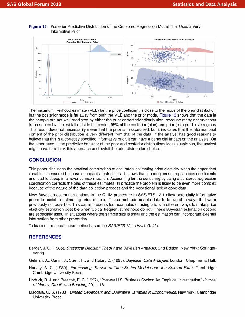
Figure 13 Posterior Predictive Distribution of the Censored Regression Model That Uses a VeryInformative Prior

The maximum likelihood estimate (MLE) for the price coefficient is close to the mode of the prior distribution,but the posterior mode is far away from both the MLE and the prior mode. Figure 13 shows that the data inthe sample are not well predicted by either the prior or posterior distribution, because many observations(represented by circles) fall outside the central 95% of the posterior (blue) and prior (red) predictive regions.This result does not necessarily mean that the prior is misspecified, but it indicates that the informationalcontent of the prior distribution is very different from that of the data. If the analyst has good reasons tobelieve that this is a correctly specified informative prior, it can have a beneficial impact on the analysis. Onthe other hand, if the predictive behavior of the prior and posterior distributions looks suspicious, the analystmight have to rethink this approach and revisit the prior distribution choice.

CONCLUSION

This paper discusses the practical complexities of accurately estimating price elasticity when the dependentvariable is censored because of capacity restrictions. It shows that ignoring censoring can bias coefficientsand lead to suboptimal revenue maximization. Accounting for the censoring by using a censored regressionspecification corrects the bias of these estimates. In practice the problem is likely to be even more complexbecause of the nature of the data collection process and the occasional lack of good data.

New Bayesian estimation options in the QLIM procedure in SAS/ETS 12.1 allow potentially informativepriors to assist in estimating price effects. These methods enable data to be used in ways that werepreviously not possible. This paper presents four examples of using priors in different ways to make priceelasticity estimation possible when typical frequentist methods do not. These Bayesian estimation optionsare especially useful in situations where the sample size is small and the estimation can incorporate externalinformation from other properties.

To learn more about these methods, see the SAS/ETS 12.1 User’s Guide.

REFERENCES

Berger, J. O. (1985), Statistical Decision Theory and Bayesian Analysis, 2nd Edition, New York: Springer-Verlag.

Gelman, A., Carlin, J., Stern, H., and Rubin, D. (1995), Bayesian Data Analysis, London: Chapman & Hall.

Harvey, A. C. (1989), Forecasting, Structural Time Series Models and the Kalman Filter, Cambridge:Cambridge University Press.

Hodrick, R. J. and Prescott, E. C. (1997), “Postwar U.S. Business Cycles: An Empirical Investigation,” Journalof Money, Credit, and Banking, 29, 1–16.

Maddala, G. S. (1983), Limited-Dependent and Qualitative Variables in Econometrics, New York: CambridgeUniversity Press.

13


ACKNOWLEDGMENTS

The authors are grateful to Anne Baxter and Ed Huddleston at SAS Institute Inc. for their valuable assistancein the preparation of this paper.

CONTACT INFORMATION

Your comments and questions are valued and encouraged. Contact the author:

Christian MacaroSAS Institute Inc.SAS Campus DriveCary, NC [email protected]

SAS and all other SAS Institute Inc. product or service names are registered trademarks or trademarks ofSAS Institute Inc. in the USA and other countries. ® indicates USA registration.

Other brand and product names are trademarks of their respective companies.

14


448-2013: estimating censored price elasticities … 448-2013 estimating censored price elasticities...

Documents