4 rotations - instituto nacional de matemática pura e...

4 Rotations

The space of rotations has great importance in Computer Graphics. Examples of appli-cations include animation of rigid bodies, linked hierarchies, as well as the specificationof external parameters for orientation and position of the virtual camera:

In this chapter, we are interested on two problems:

“to obtain good representations and parameterizations of the space of rota-tions.”

In general, a good representation leads to a good parameterization. The latter, in turn,leads to good interface solutions for the user to specify and to manipulate rotations in thecomputer:

Rotation −→ Representation −→ Parameterization −→ Specification

What is a good representation or a good parameterization as shown above? Currentliterature presents six methodologies to describe and to specify rotations in ComputerGraphics: Interpolation (e.g. keyframes in animation); Direct and inverse kinematics;Direct and inverse dynamics and Space-time optimization.

A good representation of the space of rotations should attend the requirements of theseseveral methodologies. Among them we can mention:

1. Capability of determining orientations of rigid bodies in space as a function of theparameters;

2. The possibility to calculate the parameters from a rotation;

3. The possibility to calculate the physical magnitudes of Kinematics and of theDynamics associated with a rigid body.

4. In particular, the previous item demands the possibility to (1) do calculations de-rived from the positions and orientations as a function of the parameters, (2) toobtain equations of several types (differential, integral, etc.) and (3) to solve thoseequations.

1

2 CHAPTER 4: ROTATIONS

5. Possibility to have a good control in the interpolation of rotations, by means of theinterpolation of the associated parameters;

6. The possibility to do operations among rotations either in the parameters or therepresentation space.

We begin our study with a brief discussion about rotations on the plane.

1 Rotations in the Euclidean Plane

The space of rotations in the plane is indicated by SO(2) and it is called two-dimensionalspecial orthogonal group. Given an orthonormal basis β = {b1,b2} of the plane, therotation R that carries the canonical basis {e1, e2} to basis β is defined by the angle θbetween vectors e1 and b1, as shown in Figure 1(a). The matrix of R is given by

R(θ) =(

cos θ − sin θsin θ cos θ

). (4.1)

Therefore, we have a natural parameterization of R : R → SO(2), R = R(θ). How-ever, the parameterization is not injective because R(θ) = R(θ + 2kπ). We can havebijectivity by restricting the domain to the interval [0, 2π).

Instead of using matrices, we can represent the space SO(2) using complex numbers.In fact, given an arbitrary point p = (x, y) of the plane, we identify p with the complexnumber x+ iy. We can then write p in its polar form,

p = reiθp = r cos θp + ri sin θp,

where r =√x2 + y2 is the norm of p, and θp = arctg(y/x) is the angle from p with

the x-axis (see Figure 1 (b)). When r = 1, we say the complex number is unit. In this

θ

e

e

b

b

(a)

θ

x

y

(b)

Figure 1. Rotation of the plane (a); complex number (b).

SECTION 1: ROTATIONS IN THE EUCLIDEAN PLANE 3

way, an unit complex number z can be written in the form

z = eiθz = cos θz + i sin θz.

Hence, the product of p by the unit complex z is given by

pz = zp = rei(θz+θp).

Therefore, pz is the point in the plane obtained by rotating p by an angle θz about theorigin.

Therefore, we define a biunivoc application ϕ : S1 → SO(2), representing a rotationof an angle θ by the complex unit number z = eiθ. More precisely, we associate thethe rotation ϕ(z) to the complex number z ∈ S1 such that ϕ(z).p = zp = pz. It iseasy to verify that ϕ(z).p = zp = pz. In other words, the product of complex numbersin S1 corresponds to the (composed) product of rotations. Therefore we can work withrotations in the plane using unit complex numbers.

The linear interpolation of two rotations z1 = R(θ1) = eiθ1 and z2 = R(θ2) = eiθ2

can be obtained for the complex number, in an elegant way,as follows

R(t) = ei[(1−t)θ1+tθ2], t ∈ [0, 1].

It is easy to verify that the above interpolation equation can still be written in a brieferalgebraic way:

R(t) = (z2z−11 )tz1, t ∈ [0, 1].

The representation of a rotation in the plane by a complex number allows obtaining aparameterization of the space SO(2) defining the exponential application exp: R→ S1,for

exp(t) = eit = cos t+ i sin t.

Geometrically, this application is defined in the straight tangent line to S1 in the point(0, 1). It applies each real number t in the extreme point of the arch length |t| going frompoint (0, 1) to point (cos t, sin t) in the circle (see Figure 2). Notice that the exponentialis biunivoc in the interval (−π, π)

In summary, the representation of rotations by complex numbers is very convenient,and it brings several advantages in relation to matrix representation. Amongst them, wecan mention:

• A 2 × 2 matrix (4 components) occupies more storage space of than a complexnumber (2 components).

• The number of operations to multiply two complex numbers (4 products) is smallerthan the number of operations to multiply a matrix by a vector (8 products).


exp(t)

t

t

0

Figure 2. Exponential application.

Finally, we do not obtain a good result using matrix representation to compute interpo-lation of rotations: the interpolated matrix

R(t) = (1− t)(

cos θ1 − sin θ1sin θ1 cos θ1

)+ t

(cos θ2 − sin θ2sin θ2 cos θ2

).

do not represent, in general, even a rotation in the plane.Those facts show the representation by complex numbers is superior to the represen-

tation of rotations by matrices. The study of the space of rotations in R3 is well morecomplex than the two-dimensional case seen above. However, we will see that the re-sults of this section admit a good amount of generalization by substituting the complexnumbers for another set with a similar algebraic structure: the Hamilton quaternions.

2 Rotations in the Euclidean Space

Let E = {e1, e2, e3} be the canonical basis of the Euclidean space R3 and F ={f1, f2, f3} an orthonormal basis. The change of basis T : R3 → R3, T (ei) = fi de-fines an orthogonal transformation. If the determinant of T is positive, then F has thesame orientation of E and the transformation T is said to be positive. The space of thepositive orthogonal transformations is indicated by SO(3), and it is called orthogonalspecial group of order 3.

A rigid body does not suffer deformations when moving in the space. Therefore, itspositioning is completely determined for a reference frame {O, f1, f1, f3} attached to it(local reference frame). The origin O of the reference frame supplies the position of therigid body, and the basis {f1, f1, f3} defines its orientation. Therefore, the orthogonaltransformations determine the orientation of a rigid body in space.

Our goal is to understand the space SO(3). We can state an important first topologicalresult one about this space:

“The space SO(3) is compact.”

SECTION 3: THE SPACE OF ROTATIONS 5

In fact, it is closed because it is a subset of matrices with determinant 1, and it is limitedonce the columns of a matrix in SO(3) have norm equal to 1.

We will look for a better understanding of the topology and of the geometry of thatspace to obtain good representations and parameterizations. An important result in thisdirection is given by

Theorem 1. If R is an element of SO(3), there is an orthonormal basis of R3 in whichthe matrix of R has the form 1 0 0

0 cos θ − sin θ0 sin θ cos θ

. (4.2)

Geometrically, the theorem affirms that a positive orthogonal transformation is givenby one rotation of an angle θ about an axis (the defined axis for the first vector of thebasis). The above theorem is known in Mechanics as Euler’s Theorem1:

“Every orientation is defined by a rotation about an axis.”

Euler’s Theorem extends for orthogonal transformations in Rn. A detailed discussioncan be found in (Lima, 1999). From now on we will refer to SO(3) as space of rota-tions.To understand geometrically the rotations of R3 and to look for tools for a correctmanipulation are well more difficult than one could imagine at first view. Let us see onesimple example to convince us.

Example 1. The set of rotations SO(3), with the usual operation of matrix multiplication,has a group structure. In fact, it is easy to verify that the product of positive orthogonaltransformations is orthogonal and positive as well. Therefore, if R1 and R2 are rotationsabout an r1 and r2 axes, respectively, the product R1R2 is also a rotation. Question:What is the rotation axis of the product?

3 The space of rotations

Previously, we saw that the space of rotations in the plane is naturally identified withthe circle S1, which is naturally embedded in the R2. In reality, this is the topologicalfact that allowed us to obtain a good representation of rotations in the plane. A questionappears in a natural way:

“Can we represent the space SO(3) by a surface S ⊂ R3?”

We will make a first intuitive attempt for answering the above question. From Euler’stheorem, a rotation is determined by an axis, which in turn is completely determined by

1Leonhard Euler (1707-1783), Swiss Mathematician.


a unit vector in R3. Therefore, the set of the axes is naturally identified with the unitsphere in R3:

S2 = {(x, y, z) ∈ R3;x2 + y2 + z2 = 1}.

Besides an axis, we also need a rotation angle, that is one more degree of freedom. Wetherefore see the space of rotations having dimension 3: two degrees of freedom to choosethe axis, and one more degree of freedom to choose the rotation angle about the axis 2.

The fact that space SO(3) has dimension 3 indicates some difficulty in its study. In fact,in the case of the plaen we saw that SO(2) has dimension 1 and it is naturally embeddedin R2. It is topological fact that the tridimensionality of SO(3), together with his fact itis compact, shows that it cannot be embedded in R3. This means that, topologically, therotations of the R3 space do not belong to R3 and we should look for one representationin spaces of larger dimension.

We begin our search with the matrix representation of SO(3).

3.1 Representation by matrices with linkage

We know that a rotation that takes the canonical basisE = {e1, e2, e3} of R3, in anotherpositive orthonormal basisF = {f1, f2, f3} becomes completely determined by the matrixf11 f12 f13

f21 f22 f23

f31 f32 f33

,

where T (ei) =∑3

j=1 fjifj .Therefore, in a first inspection, we can parameterize the space of orientations using

3 × 3 matrices. In this case, ee would have a representation naturally embedded in theR9 (9 degrees of freedom). However, it occurs that the columns of the above matrix arethe coordinates of the vectors fi that form an orthonormal basis. Therefore,

|fj |2 =3∑j=1

f2ij = 1, j = 1, 2, 3. (4.3)

and

〈fi, fj〉 =3∑i=1

fijfik = 0, j 6= k, j, k = 1, 2, 3. (4.4)

These six equations reduce the degrees of freedom of choosing the matrix of T from9 for 3. (In reality, we are defining the space of rotations implicitly in R9.)3 Working

2In an intuitive way, we have two degrees of freedom by pointing our arm in a direction in space, we stillhave a degree of freedom by rotating the arm longitudinally.

3Note we have here another demonstration that SO(3) has dimension 3.

SECTION 4: PARAMETERIZATION BY EULER’S ANGLES 7

with such matrix representation has always the problem of guaranteeing that the matricesunder consideration satisfy to the six linkage conditions from equations (4.3) and (4.4).That is a difficult problem and computationally costly.

We will continue with our search by describing a local parameterization of the spaceof rotations which is very used in the Mechanics, and it was discovered by LeonhardEuler.

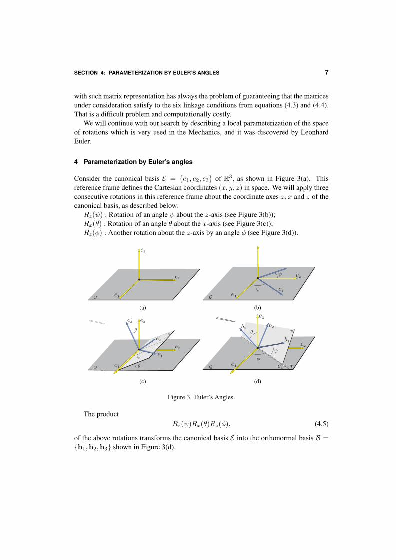
4 Parameterization by Euler’s angles

Consider the canonical basis E = {e1, e2, e3} of R3, as shown in Figure 3(a). Thisreference frame defines the Cartesian coordinates (x, y, z) in space. We will apply threeconsecutive rotations in this reference frame about the coordinate axes z, x and z of thecanonical basis, as described below:Rz(ψ) : Rotation of an angle ψ about the z-axis (see Figure 3(b));Rx(θ) : Rotation of an angle θ about the x-axis (see Figure 3(c));Rz(φ) : Another rotation about the z-axis by an angle φ (see Figure 3(d)).

e

Q

(a)

e

Qψ

ψ

(b)

θ

e

Q

ψ

θ

eP

(c)

θ

r

e

ψ

φ

P

Q

(d)

Figure 3. Euler’s Angles.

The productRz(ψ)Rx(θ)Rz(φ), (4.5)

of the above rotations transforms the canonical basis E into the orthonormal basis B ={b1,b2,b3} shown in Figure 3(d).


Now let us suppose the orthonormal reference frame B = {b1,b2,b3} is given apriori. Statement: ” the reference frame B can be obtained from the canonical basis Eby three consecutive rotations ”. In fact, as we showed in Figure 3(d), let P be the planegenerated by the vectors b1 and b2 of the basis B, and r the intersection straight linebetweenP with the plane z = 0 (r is called nodal straight line in Mechanics). Notice thatthe unit vector e3 ∧b3 points towards the direction of the nodal straight line. (In fact, e3

and b3 are normal to the planes z = 0 and P , respectively. Therefore, the cross producte3 ∧b3 should point towards the direction of the intersection straight line between thesetwo planes, which is the nodal straight line.) Let us also indicate by φ the angle betweenthe vector e1 and the nodal straight line.

Initially we do a rotationRe3(φ), of an angle φ about the axis e3, that takes the vectore1 into the vector e′1 = e3 ∧ b3. Soon afterwards, we apply the rotation Re3∧b3(θ),by an angle θ about the nodal straight line, which takes the vector e3 into the vector b3.Finally, we apply the rotationRb3(ψ), by an angle ψ about the vector b3 which takes thevector e′1 into the vector b1. Of course, this sequence of rotations

Re3(φ)Re3∧b3(θ)Rb3(ψ), (4.6)

transforms the canonical basis into the basis B.Notice that the transformation in (4.5) is equal to the one in (4.6) because both coincide

in the canonical basis E . However, they apply the rotations in inverse order and withdifferent axes. In the first case, the rotations are always done around the axes of theCartesian (global) system; In the second case, the rotations are applied consecutively inlocal coordinate systems (except for Re3(φ), of course).

We know that a rotation R in space is determined for the positive orthonormal basisB = {b1,b2,b3}. (The rotation is given by the linear transformation taking the canonicalbasis E = {e1, e2, e3} into the basisB). Therefore, we showed above the following result:

“A rotationR ∈ SO(3) can be obtained by three consecutive rotations aboutthe coordinate axes.”

This result is owed to Leonhard Euler, and the angles (φ, θ, ψ) are called Euler’sangles. They constitute a parameterization of the space SO(3). This parameterization isused broadly in the study of rigid bodies dynamics in R3.

4.1 Yaw, Pitch and Roll

In the previous section, we saw two different choices of parameterizations by Euler’sangles, with different rotation axes and order about them. The parameterization of SO(3)using Euler’s angles is broadly used in the Computer Graphics aiming at specifyingrotations. It is common to use names brought from aviation: yaw (deflection angle),

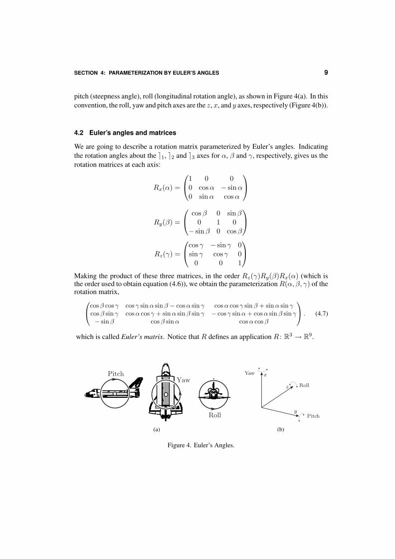
SECTION 4: PARAMETERIZATION BY EULER’S ANGLES 9

pitch (steepness angle), roll (longitudinal rotation angle), as shown in Figure 4(a). In thisconvention, the roll, yaw and pitch axes are the z, x, and y axes, respectively (Figure 4(b)).

4.2 Euler’s angles and matrices

We are going to describe a rotation matrix parameterized by Euler’s angles. Indicatingthe rotation angles about the e1, e2 and e3 axes for α, β and γ, respectively, gives us therotation matrices at each axis:

Rx(α) =

1 0 00 cosα − sinα0 sinα cosα

Ry(β) =

cosβ 0 sinβ0 1 0

− sinβ 0 cosβ

Rz(γ) =

cos γ − sin γ 0sin γ cos γ 0

0 0 1

Making the product of these three matrices, in the order Rz(γ)Ry(β)Rx(α) (which isthe order used to obtain equation (4.6)), we obtain the parameterizationR(α, β, γ) of therotation matrix,cosβ cos γ cos γ sinα sinβ − cosα sin γ cosα cos γ sinβ + sinα sin γ

cosβ sin γ cosα cos γ + sinα sinβ sin γ − cos γ sinα+ cosα sinβ sin γ− sinβ cosβ sinα cosα cosβ

. (4.7)

which is called Euler’s matrix. Notice that R defines an application R : R3 → R9.

Pitch

Roll

Yaw

(a)

y

z Roll

Pitch

Yaw x

(b)

Figure 4. Euler’s Angles.


4.3 Singularities and Euler’s angles

Euler’s angles do not constitute a global parameterization of the space of rotations. Thereason being the space SO(3) is compact, and therefore it cannot be parameterized byan open set of R3 (in the same way a sphere S2 ⊂ R3 does not admit a global parame-terization for an open subset in the plane). In this way, any attempt of extending Euler’sangles to cover the whole space of rotations leads to the creation of singularities in theparameterization. These singularities are regions in the domain of the parameterizationin which we do not have the three degrees of freedom in the rotation matrix (see the dis-cussion of singularity in the parameterization of the sphere in the chapter on coordinatesystems).

We can describe singularities of the parameterization for Euler’s angles by takingβ = π/2 in the parameterization R(α, β, γ) of equation (4.7). That is, doing a rotationof 90◦ about the y-axis (pitch), we obtain the parameterization

R(α,π

2, γ) =

0 cos γ sinα− cosα sin γ cosα cos γ + sinα sin γ 00 cosα cos γ + sinα sin γ cosα sin γ − cos γ sinα 0−1 0 0 0

=

0 sin(α− γ) cos(α− γ) 00 cos(α− γ) sin(α− γ) 0−1 0 0 0

.

We see that, despite having two degrees of freedom in the parameter space, we havejust one degree of freedom in the parametrization. This is because the parametrizedmatrix only depends on the difference of the angles. (This phenomenon is similar to thesingularity in the parameterization of the sphere that we saw in the chapter of coordinatesystem.)

It is easy to understand intuitively the singularities of the parameterization of SO(3)using Euler’s angles. In fact, the angles perform three consecutive and independentrotations in each one of the coordinate axes: first we rotate about z, then about y, andlater about x. The singularities happen as two axes of rotation point towards the samedirection. This is because the rotations about those two axes are dependent and thereforewe loose a degree of freedom.

The gimbal lock phenomenon

The problem of singularities of Euler’s angles manifests in practice. The phenomenon isknown in Aeronautical Engineering and Mechanical Engineering as gimbal lock 4.

4Gimbal is the given name to the mechanical assembly of equipments requiring a space orientation and,for that end, using Euler’s angles: for example, gyroscope, optic equipments

SECTION 5: INTERPOLATION OF ROTATIONS 11

Roll

Pitch

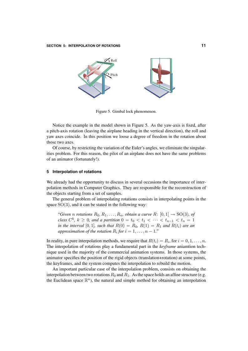
Figure 5. Gimbal lock phenomenon.

Notice the example in the model shown in Figure 5. As the yaw-axis is fixed, aftera pitch-axis rotation (leaving the airplane heading in the vertical direction), the roll andyaw axes coincide. In this position we loose a degree of freedom in the rotation aboutthose two axes.

Of course, by restricting the variation of the Euler’s angles, we eliminate the singular-ities problem. For this reason, the pilot of an airplane does not have the same problemsof an animator (fortunately!).

5 Interpolation of rotations

We already had the opportunity to discuss in several occasions the importance of inter-polation methods in Computer Graphics. They are responsible for the reconstruction ofthe objects starting from a set of samples.

The general problem of interpolating rotations consists in interpolating points in thespace SO(3), and it can be stated in the following way:

“Given n rotations R0, R1, . . . , Rn, obtain a curve R : [0, 1] → SO(3), ofclass Ck, k ≥ 0, and a partition 0 = t0 < t1 < · · · < tn−1 < tn = 1in the interval [0, 1], such that R(0) = R0, R(1) = R1 and R(ti) are anapproximation of the rotation Ri for i = 1, . . . , n− 1.”

In reality, in pure interpolation methods, we require thatR(ti) = Ri, for i = 0, 1, . . . , n.The interpolation of rotations play a fundamental part in the keyframe aniamtion tech-nique used in the majority of the commercial animation systems. In those systems, theanimator specifies the position of the rigid objects (translation+rotation) at some points,the keyframes, and the system computes the interpolation to rebuild the motion.

An important particular case of the interpolation problem, consists on obtaining theinterpolation between two rotationsR0 andR1. As the space holds an affine structure (e.g.the Euclidean space Rn), the natural and simple method for obtaining an interpolation


Figure 6. Moving a boomerang by interpolating Euler’s angles.

between two objectsR0 andR1 is a linear interpolation, defined asR(t) = (1− t)R0 +tR1, t ∈ [0, 1].

In the case R0 and R1 are matrices, then linear interpolation makes sense, becausethe space of matrices is a vector space. However, if R0 and R1 are rotation matrices, thematrix R(t) = (1− t)R0 + tR1, t ∈ [0, 1], in general does not represent a rotation. Thishappens because the space of rotations SO(3) is not a linear subspace of matrix space.(The problem here is similar to a linear interpolation between two points on a sphere: theresulting segment is not contained in the sphere.)

5.1 Interpolating Euler’s angles

When we have a parameterization ϕ : U ⊂ Rm → S of a space S, the interpolationproblem is reduced to interpolate in the parameters space U . In fact, to interpolate npoints p1, . . . ,pn ∈ S, we take the corresponding points ϕ−1(p1), . . . , ϕ−1(pn), in theparameters spaceU ⊂ Rn, and we obtain an interpolation curve c : [0, 1] : → Rm amongthose points. The desired interpolation curve is given by the composite ϕ◦c : [0, 1]→ S.Therefore, the interpolation problem is reduced to one in Rm, which is broadly coveredin the literature.

In particular, the above principle is applied to interpolate rotations using the pa-rameterization by Euler’s angles as shown in Figure 6. In this case, if we have tworotations R0 = R(α0, β0, γ0) and R1 = R(α1, β1, γ1), we obtain a curve c in the pa-rameters space, c(t) = (α(t), β(t), γ(t)), such that c(0) = (α(0), β(0), γ(0)) = R0 andc(1) = (α(1), β(1), γ(1)) = R1. The interpolating path in SO(3) is given by the com-posite R(t) = R(α(t)), R(β(t)), R(γ(t)), whereR = Rαβγ is the Euler matrix given inthe equation (4.7). (we can of course use this method to interpolate n rotations.)

The advantage of this method is that the interpolation itslef is done in the R3 space.In this way, we can interpolate an arbitrary number of rotations using the various pointinterpolation methods of interpolation described in the literature (e.g. Splines, Bezier,Hermite). This method is, of course, applicable to any other parameterization of the space

SECTION 6: PAUSE FOR COMMERCIALS 13

of rotations.The interpolation of Euler’s angles is the method used in the majority of keyframe

animation systems to specify the orientation of the objects and of the virtual camera. Thedisadvantages of this method are all those inherent to the parameterization method withEuler’s angles that we will discuss next.

6 Pause for commercials

The parameterization of the space of rotations using Euler’s angles is broadly used inthe area of Animation. A sequence of rotations with Euler’s angles is represented by athree-dimensional curve where each component represents a rotation angle in each axis.Therefore, the animators work by manipulating curves in the R3 space to modify path,speed, acceleration etc. In general, the editing is made over the projection of these curvesin the coordinate planes, an interface in which animators are already quite familiar with.

Another advantage of matrices, and in particular of Euler matrices, is that other pro-jective transformations are also represented by matrices, especially translation.

However, besides the problem of singularities (gimbal lock), discussed above, theparameterization for Euler’s angles has several other inconvenients.

Given a rotation matrix, we can have ambiguities in the solution of the inverse problem.What are the axis and rotation angle?

The representation for Euler’s angles has no unicity because it depends on the orderof the axes (anisotropy);

The parameterization defines a local coordinate system in the space of rotations; Inother words, we cannot describe all rotations using just an Euler coordinate system. Ofcourse, we can use several parameterizations to cover the SO(3) space; However, it isnot simple to perform a change of coordinates between two systems of Euler’s angles.

Finally, specifying rotations using Euler’s angles is difficult and not intuitive. Let ussee a practical example: hold a football ball, mark a point on it with a pen and rotate it toplace the marked point in the vertical position (north pole of the ball). Easy, right? Nowtry to solve the same problem with three successive rotations about the axes accordingto Euler’s parameterization. In the first solution, in an intuitive and natural way, we usedEuler’s Theorem, by doing a single rotation about an axis.

The above fact shows that we should look for a representation of SO(3) where eachrotation is represented by its axis, together with the rotation angle. To have this intuitiverepresentation mathematically efficient, we need to introduce a mathematical structurein space constituted by the elements ” axis + rotation angle ”. This will be our goal inthe remaining of this chapter.


7 Quaternions

Quaternions introduce an algebraic structure in the Euclidean space R4 similar to thestructure of the complex numbers in the R2 plane. This structure allows to obtain arepresentation of the space of rotations based on the ” axis+angle ”model to define arotation.

We denote as {1, i, j,k} the canonical basis of the space R4: 1 = (1, 0, 0, 0), i =(0, 1, 0, 0), j = (0, 0, 1, 0) and k = (0, 0, 0, 1). A point p = (w, x, y, z) ∈ R4 is thenwritten in the form p = w + xi + yj + zk. Amongst the four elements 1, i, j and k ofthe basis, we define a product according to the table below:

· 1 i j k1 1 i j ki i -1 k −jj j -k -1 ik k j -i -1

Table 1: Multiplication of the quaternions in the basis.

Notice that the product is not commutative. We extended the above product to obtainthe product pq between two arbitrary points of R4 requiring bilinearity. In other words,if p1,p2,q1,q2 ∈ R4, we have

(ap1 + p2)(bq1 + q2) = abp1q1 + ap1q2 + bp2q1 + p2q2.

The space R4, with the above multiplicative structure, is called quaternions spaceor simply quaternions. Quaternions were discovered by William Hamilton5 with thegoal of obtaining in the space the same relation between rotations and complex numbersthat exists in the plane. The operation of quaternion product is distributive, associative(tedious check), and, highlighting once again, not commutative.

The subspace R1 = {(x, 0, 0, 0);x ∈ R} is identified with the set of the real numbers,and it is called space of scalars; the subspace R i+R j+Rk = {(0, x, y, z);x, y, z ∈ R}is naturally identified with the Euclidean space R3 and it is called space of vectors orspace of pure quaternions. Given a quaternion u ∈ R4, u = w + xi + yj + zk, thenumber w is called real part of u and it is indicated by <(u); the vector xi + yj + zk,is called of vector part of u. If v = (x, y, z) ∈ R3 is a vector, we indicate by v theassociated pure quaternion: v = xi + yj + zk. In this way, every quaternion can bewritten in the form p = w + v, w ∈ R, v ∈ R3.

5Sir William Rowan Hamilton (1805-1865), Irish mathematician.

SECTION 7: QUATERNIONS 15

The conjugated of a quaternion u = w+ v is defined by u? = w− v. In other words,if u = w+xi+yj+zk, then u? = w−xi−yj−zk. The conjugation operation satisfiesthe properties (u?)? = u and (uv)? = u?v?. Of course, the real part of a quaternion uis equal to <(u) = (u + u?)/2.

The norm of a quaternion p = w + xi + yj + zk is equal to the norm of the vector(w, x, y, z) in the Euclidiano inner product of R4:

|p| =√〈p,p〉 =

√w2 + x2 + y2 + z2.

Of course if p = w + v then |p|2 = w2 + |v|2.Also, |p| = |p?|. The norm behaves well in relation to the quaternion product (verify):

|p1 p2| = |p1||p2|. (4.8)

If |p| = 1, we say p is a unit quaternion. Of course, the set of unit quaternions form theunit sphere S3 ⊂ R4,

S3 = {(w, x, y, z) ∈ R4;w2 + x2 + y2 + z2 = 1}.

Besides, for (4.8), the product of two unit quaternions is a unit quaternion. Therefore,S3 is a group, as seem as the set of unit quaternions. (Notice here the analogy with thecircle S1 ⊂ R2 that is a group formed by the complex numbers of norm 1.)

The multiplicative inverse of a quaternion u, is a quaternion u−1 such that uu−1 =u−1u = 1. An immediate calculation shows that every nonull quaternion u has onemultiplicative inverse given by

u−1 =u?

|u|2,

Notice if |u| = 1, then u−1 = u?.If q1 = a1 + v1 and q2 = a2 + v2, a direct calculation shows that the product of q1

and q2 is given by

q1q2 = a1a2 − 〈v1, v2〉+ a1v2 + a2v1 + v1 ∧ v2.

We are using the notation v1 ∧ v2 to indicate v1 ∧ v2. Therefore, if q1 and q2 are purequaternions, that is, a1 = a2 = 0, then

q1q2 = −〈v1, v2〉+ v1 ∧ v2.

Therefore, the quaternion product synthesizes two types of vector products in R3: thescalar and cross products (in a way this let us foresee the great potential of this operation).Notice if v is a pure quaternion, v ∧ v = 0, and by taking q1 = q2 = v in the previousequation, we obtain

v2 = −〈v,v〉 = −||v||2.


In particular, if v is a unit pure quaternion, we have v2 = −1.Every quaternion q = a + v can be written in the form a + bu, where |u| = 1 is a

unit quaternion. In fact, we can only take

u =v|v|, e b = |v|.

Observe that the representation of a quaternion in the form q = a+ bu, as |u| = 1, thatis, u is a pure unit quaternion, we have u2 = −1. Yet, in this representation, if q is unit,we have

1 = |q|2 = a2 + b2|u|2 = a2 + b2.

Therefore, there exists θ ∈ R such that a = cos θ and b = sin θ, and we can writeq = cos θ + sin θ u.

Notice the similarity of what we have obtained above with the complex numbers. Acomplex number has the form x+ iy with i2 = −1; Besides, every unit complex number,i.e. of norm 1, can be written in the form cos θ + i sin θ. The difference is that, unlikethe complex number i, the unit quaternion u, in the representation p = a+ bu, dependson the quaternion p.

The results here show that quaternions have algebraic properties similar to the onesin complex numbers, with exception for commutativity. Our final test is to try to extendthe result involving complex numbers and rotations of the plane to quaternions. This isthe subject of the next section.

7.1 Representation of rotations by quaternions

Given a unit quaternion q, we should define the transformation Rq : R4 → R4 placingRq(p) = pq. We have |Rq(p)| = |p||q| = |p|, therefore the transformation Rq isorthogonal. That is, multiplications for unit quaternions geometrically correspond torotations in R4 space. Now, a natural question comes into play:

“How to obtain a representation of SO(3) by quaternions?”

A first idea would be to associate, to each quaternion q ∈ R3, the transformation Rq.Unfortunately, in general, Rq /∈ SO(3), that is, the space of pure quaternions, naturallyidentified with R3, is not invariant for Rq. The representation of SO(3) by quaternionsis a little subtler as we will see.

Observe that the representation of a unit quaternion q in the form q = cos θ+sin θ u,with |u| = 1, shows this quaternion defines an angle θ and an axis u of the space. It isnatural to expect this quaternion to represent a rotation about the u-axis . We will showthis in fact happens and the angle of that rotation is 2θ.

Given a unit quaternion q, we define the transformation ϕq : R3 → R3, placing

ϕq(v) = qvq−1 = qvq?, v ∈ R3. (4.9)


We will demonstrate several properties soon afterwards of that transformation.the transformation ϕq is well defined. This means ϕq(v) ∈ R3. For that, it is enough

to show <(ϕq(v)) = 0:

<(qvq−1) = <(qvq?);= [qvq? + (qvq?)?]/2;= [qvq? + qv?q?]/2;= q[(v + v?)/2]q?;= q<(v)q? = <(v)qq? = <(v) = 0.

The transformation ϕq is linear. In fact,

ϕq(au + v) = q(au + v)q?

= qauq? + qvq?

= a(quq?) + (qvq?)= aϕq(u) + ϕq(v).

The transformation ϕq is orthogonal. In fact,

|ϕq(v)| = |qvq?| = |q||v||q?| = |v|.

The transformation ϕq is a rotation of R3. In fact, as we saw above, it is enough toshow ϕq is positive. In this case, notice for q = 1 ϕq = I , where I : R3 → R3 is theidentity transformation. As the space of unit quaternions is connected (because it is theunit sphere in R4), we conclude by a continuity argument that ϕq is positive for everyquaternion q. The axis of rotation of ϕq is the quaternion u. In fact, it is enough showthat ϕq(u) = u:

ϕq(u) = quq?

= (cos θ + u sin θ) u (cos θ − u sin θ)

= (cos θ)2u− (sin θ)2u3

= (cos θ)2u− (sin θ)2(−u)= u.

The angle of rotation of ϕq is 2θ. We will make a geometric demonstration of thisfact, by solving the following problem:

“Given a rotation R of an angle θ about an axis r, how can we obtain thequaternion q of the representation ϕq in R?”


O

P P

H V

Figure 7. Rotation of an angle θ about the axis defined by vector n

To answer the above question, consider Figure 7 showing the rotation R of point P byan angle β about the OH-axis. The image of point P is the point P ′ = R(P ).

Let us take the positive reference frame {u,v,n}, where u =−−→HP , v =

−−→HV and n

is the unit vector in the direction of the rotation axis. We also define the vectors

h =−−→OH, p =

−−→OP, p′ =

−−→OP ′, and u′ =

−−→HP ′.

with u ⊥ h, h ⊥ v and |v| = |u|. Having h as the orthogonal projection of p in thedirection n, we have h = 〈p,n〉n. It is also easy to verify that

p′ = h + u′

u = p− h = p− 〈p,n〉nu′ = cosβu + sinβ v,

and besides,

v = n ∧ u = n ∧ (p− h) = n ∧ (p− 〈p,n〉) = n ∧ p.

We then have

R(P ) =−−→OP ′ = h + u′

= 〈n,p〉n + cosβu + sinβv= 〈n,p〉n + cosβ(p− 〈p,n〉n) + sinβ n ∧ p

= cosβp + (1− cosβ)〈n,p〉n + sinβ n ∧ p.

(4.10)

We will now calculate R(P ) using the rotation ϕq in (4.9). In this case point P isrepresented by the pure quaternion, P = p, and q is the unit quaternion q = cos θ +


n sin θ. To simplify the calculations let us take c = cos θ and t = n sin θ, thereforeq = c+ t. We then have

R(P ) = ϕq(p) = qpq?

= (c+ t)(p)(c− t)

= (c+ t)(〈p, t〉 − p ∧ t + cp)

= c〈p, t〉 − 〈t,−p ∧ t〉 − c〈t, p〉++ t ∧ (−p ∧ t) + c(t ∧ p) + c(−p ∧ hatt + cp) + 〈p, hatt〉hatt)

= 〈hatt, p〉hatt− 〈hatt, hatt〉p + 2c(hatt ∧ p) + c2p + 〈p, hatt〉hatt)= (c2 − 〈hatt, hatt〉)p + 2〈p, hatt〉hatt + 2c(hatt ∧ p).

(4.11)Substituting the values of c = cos θ and t = n sin θ, in the expression of ϕq(p)

obtained in equation (??), we have

R(P ) = (cos2 θ − sin2 θ)p + 2 sin2 θ〈p, n〉n + 2 sin θ cos θ(n ∧ p)= cos 2θp + (1− cos 2θ)〈n, p〉n + sin 2θ(n ∧ p)).

Comparing this equation with (4.10) we see that ϕq(p) is a rotation of an angle 2θ aboutthe axis defined by the unit vector n.

The results demonstrated above can be summarized in

Theorem 2 (Representation of rotations for quaternions). A rotation of an angle 2θabout an axis defined by a unit vector n is represented by ϕq(v) = qvq−1, whereq = cos θ + n sin θ.

Therefore, we have a transformation ϕ : S3 → SO(3), ϕ(q) = ϕq, representing therotations in space for points of the unit sphere in R4. Following up, from the definitionof ϕq, we have ϕq = ϕ−q. Geometrically, this fact is obvious because a rotation of anangle θ about the n-axis is the same to a rotation of an angle 2π − θ about the −n-axis.Therefore, the transformation ϕq is not injective. However, it can be shown, without alot of difficulty, that

ϕq1 = ϕq2 ⇔ q1 = ±q2.

We left that demonstration for the exercises at the end of this chapter.The above result shows that only the antipode points of the sphere define the same

rotation. Therefore, the space SO(3) is identified naturally with the unit sphere S3 inR4 with the antipode points identified. We know this is the real projective space ofdimension 3, RP3. We will not use, however, this association between SO(3) and RP3.The important aspect of the above result is that space SO(3) of the rotations can berepresented by unit quaternions. Care should only be taken with antipode points of thesphere representing the same rotation.


An important fact in relation to the representation of rotations in SO(3) by quaternions,is the product operation is preserved, that is

ϕu1u2 = ϕu1ϕu2 .

The check is immediate: for every vector v ∈ R3 we have

ϕu1u2(v) = u1u2v(u1u2)−1 = u1u2vu−12 u−1

1 = u1ϕu2 v u−11 = ϕu1ϕu2(v).

This fact shows we can substitute the product of two rotation matrices by the product ofthe quaternions representing them. In particular, notice this result answers a question wehad in the beginning of the chapter:

“If rotations R1 and R2 have axes defined by the unit vectors u1 and u2,respectively, then the axis of the rotation product R1R2 is the product ofquaternions u1u2.”

7.2 Exponential and logarithm

Consider a vector v ∈ R3, v 6= 0. and let v = v/|v| be the pure unit quaternion obtainedfrom v by normalization. Using the notation θ = |v|, we have v = θv. Substituting theexpression v = θv in the Taylor series of the exponential function we obtain,

ev = eθv =∞∑n=0

(θv)n

n!.

An immediate calculation, taking into account v2 = −1, gives us

ev = eθv = cos θ + v sin θ = cos |v|+ v sin |v|.

We can define the exponential exp: R3 → S3 having

exp(v) =

{cos |v|+ sin |v|v, se v 6= 0;1 = (1, 0, 0, 0) se v = 0,

where v = |v|/|v|. We will also use the notation exp(v) = ev. Notice that if v is a unitquaternion, then v = cos θ + sin θu, with |u| = 1. As |θu| = θ, we have

eθu = cos θ + sin θu,

which is a similar expression to eiθ = cos θ + i sin θ for complex numbers.


Now we can define the logarithm function log : S3 → R3, as being the inverse of theexponential. Given q ∈ S3, q = cos θ + sin θu, |u| = 1, we have

log(q) = θu ∈ R3.

It is immediate verifying elog(q) = q.It is sometimes useful to have the definition of the exponential and of the logaríthm

explicitly showing the coordinates; If u = w + xi + yj + zk ∈ S3, we can write

log(w, x, y, z) = arccos(w)(x, y, z)√x2 + y2 + z2

=arccos(w)√x2 + y2 + z2

(x, y, z).

Similarly, if v = (x, y, z) ∈ R3, we have

exp(x, y, z) =

cos(√x2 + y2 + z2) + sin(

√x2+y2+z2)√x2+y2+z2

(x, y, z), se (x, y, z) 6= 0;

(1, 0, 0, 0) if (x, y, z) = 0.

Now we can define arbitrary potencies of unit quaternions extending in a natural waythe result for complex numbers: if q is a unit quaternion and t ∈ R, we have

qt = et log q = etθu = cos(θt) + sin(θt)u. (4.12)

Observe that the expression c(t) = qt (with t varying in the interval [0, 1]) defines acurve c : [0, 1]→ S3 that ties the point c(0) = 1 = (1, 0, 0, 0) (north pole of the sphereS3) to the point c(1) = q. We will give a geometric interpretation of this curve, and atthe same time of the exponential function. For that we needed some definitions.

A maximum circle of the sphere S3 is a circle of radius 1, in other words, a circlecontained in S3 that has maximum radius. A maximum circle is obtained by the inter-section of S3 with a subspace of dimension 2 in R4. A geodesic of S3 is a maximumcircle parameterized for a curve c : [0, 1] → S3 such that the speed |c′(t)| is constant.This implicates that the image of an uniform partition of the parameter space [0, 1] resultsin an uniform partition of the maximum circle. (The geodesics are the ” straight line ”of the sphere S3 when walking between two points on the sphere; The smallest path isalways along a geodesic).

Let us return to equation (4.12), from which, geometrically, the curve c(t) = qt

represents a family of rotations about the same u-axis with given angles by 2θt. In S3,these rotations represent an arch of maximum circle connecting the quaternion c(0) = 1 tothe quaternion c(1) = q. We left as an exercise at the end of the chapter the demonstrationthat

c′(t) =d

dtqt = qt log q.

Then it is easy to verify that the curve c(t) holds the following properties:


Figure 8. Exponential application.

1. c′(0) = θu;

2. |c′(t)| = |θ|;

3. c′′(t) = kc(t), where k < 0 is a constant.

Condition 3 above shows that c(t), in fact, describes an arch of maximum circle, andcondition 2 guarantees us that c(t) is a geodesic. In short, the curve c(t) is a geodesic inS3, that begins in point 1 and ends in point q. (Of course the maximum circle described byc(t) is determined by the intersection of S3 with the two-dimensional subspace generatedby vectors 1 and q.)

The previous result provide us with a geometric description of the following exponen-tial application exp: R3 → S3 (see Figure 8): identifying the space R3 with the tangentplane to the sphere S3 in the point 1 (north pole), exp(v) is the extreme point of the archthat begins in 1, in the direction v and has length |v|.

In particular, notice the exponential here defined coincides with the exponential de-fined in Differential Geometry for any surface of Rn with the induced metric.

Exponential parameterization of SO(3)

The result of the previous section shows that the exponential here defined naturally extendsthe exponential exp: R → S1 that we defined in the beginning of the chapter. In thiscase, the exponential allowed a parameterization of the space of rotations of the planefor a subset of R. In ours case also, the exponential exp: R3 → S3 naturally defines aparameterization of the space of rotations SO(3).

Given a vector v ∈ R3, we have exp(v) = cos |v| + sin |v|u, where u = u/|u|.Therefore, exp(v) is a unit quaternion representing a rotation about the u-axis (this is thesame axis of v), of an angle 2|v|. That is, the exponential is a parameterization capturingthe essence of parameterizing the space of rotations in the {axis + angle} space, as we


promised previously: the axis is modeled by a vector, and the angle is its length (less offactor 2).

As we are parameterizing SO(3) by R3, of course, the exponential holds singularities.Using the geometric interpretation of the exponential it is easy to conclude that the spheresof radius kπ, k = 1, 2, . . . are singularities regions of this parameterization. They arethe regions of R3 mapped in the north pole or in the south pole of the sphere S3. Thesesingularities can be avoided in practice: when v approaches the sphere of radius π, wehave a rotation of an angle θ = 2|v| close to 2π, we then change for a rotation of an angle2π − θ about the −v-axis that is equivalent and far away from the singularity.

Observing the definition of exponential parameterization attentively, we notice that wecan have a problem of numerical instability in the calculation of the unit vector u = v/|v|,when v → 0. This problem can be avoided. In fact, we have

ev = cos |v|+ sin |v|u

= cos |v|+ sin |v| v|v|

= cos |v|+ sin |v||v|

v.

Now we only need to observe that sin |v||v| → 1 when |v| → 0. In reality, for implemen-

tation purpose, we can substitute this function by an approximation given by its Taylorseries:

sin tt

= 1 +t2

3!+t4

5!+ · · ·+ t2(n−1)

(2n− 1)!+ · · ·

7.3 Interpolating quaternions

In this section we will cover the topic of interpolating rotations using the representation byquaternions. We will just study the case for two rotations. Let us consider two rotationsϕu and ϕv of angles θu and θv about unit axes u and v, respectively. These two rotationsare represented by unit quaternions as indicated below:

ϕu ←→ p = eθuu = cos θu + sin θuu

ϕv ←→ q = eθvv = cos θv + sin θvv

We then haveϕu(x) = pxp∗ e ϕv(x) = qxq∗.

Quaternions p and q define an arch of maximum circle in the sphere S3 (see Figure 9(a)).Due to the representation of rotations by unit quaternions, an interpolation betweenthe rotations ϕu and ϕv is simply a curve g : [0, 1] → S3 in the sphere S3 such thatg(0) = p and g(1) = q. That is, the interpolation of rotations is reduced to a problem ofinterpolating points in S3.


Linear Interpolation

As quaternions hold the usual linear structure of R4, we can do a linear interpolationbetween p and q. More precisely, we define the quaternion

a(t) = (1− t)p + tq,

and the interpolated rotation is given by ϕa(t) where

ϕa(t)(x) = a(t)xa(t)∗.

The problem of this method is that a(t) are not unit quaternions. In fact, geometricallythey form a ” rope ” of the maximum circle of the unit sphere S3 ⊂ R4 containing thequaternions p and q (see Figure 9(b)).

We can bypass this problem by doing a spherical radial interpolation, consisting oftaking the radial projection of a(t) on the unit sphere, as shown in Figure 9(b). That is,

a(t) =a(t)|a(t)|

=(1− t)p + tq|(1− t)p + tq|

.

This method works; However, we do not have an uniform sampling in the angles evenwhen the sampling is uniform in time. (That is, the projection is a maximum circle but itis not a geodesic.) This fact can be observed in Figure 9(c). In other words, the angularspeed is variable (it accelerates and decelerates.).

Geodesic interpolation

Our goal now is to correct the problem of spherical radial interpolation and to obtaina interpolation between two quaternions in which the interpolating curve has constantangular speed, that is, an uniform sampling in time generates an uniform sampling in theangles. As we know already, it is enough to do the interpolation along a geodesic of thesphere S3 tieing quaternions p to q. This method is called geodesic interpolation.

Previously, we saw that curve c(t) = bt is a geodesic tying the north pole 1 of thesphere to quaternion b. This provides a geodesic interpolation between rotations ϕ1 andϕb.

p q

(a)

p q

(b)

p q

(c)

Figure 9. Quaternion interpolation.


How to obtain a geodesic tieing p to q? A simple calculation shows the curve

g(t) = (qp)tp, t ∈ [0, 1], (4.13)

satisfies g(0) = p and g(1) = q. It remains to show g(t) is a geodesic. For this, observethat g(t) = Rp(c(t)) where c(t) = (qp)t and Rp is the transformation of S3 defined byRp(v) = vp. Now we know c(t) is a geodesic; On the other hand, the transformationRp is orthogonal, therefore preserving geodesics for being an isometry of the sphere.(In more geometric terms: a geodesic is a maximum circle and sphere rotations preservemaximum circles.)

In conclusion, equation (4.13) defines a geodesic interpolation between quaternionsp and q. This interpolation method is called spherical linear interpolation or, briefly,slerp.

Next, we will obtain an expression of geodesic interpolation which is very common inthe literature; It expresses the interpolation parameter in terms of angles in the maximumcircle tieing p to q. Let θ be the angle between quaternions p and q, that is, cos θ = 〈p,q〉(Figure 10(a)).

(a) (b)

Figure 10. Spherical linear Interpolation.

As we will work with angles of the maximum circle, our problem is reduced to aplanar one. (That is, we work in the plane of the maximum circle, defined by p, q andthe origin). Observing Figure 10(b), we have:

p = (cos(θ0), sin(θ0)),q = (cos(θ0 + θ), sin(θ0 + θ)).

Therefore, in terms of angles, the interpolation between p and q is given by

g(t) = (cos(θ0 + tθ), sin(θ0 + tθ)).


Now we should write this expression as function of quaternions p and q. That is achievedwith a simple calculation, using trigonometry (we will indicate a vector (x, y) in the plane

by a column matrix(xy

), due to space contraints):

g(t) =(

cos(θ0 + tθ)sin(θ0 + tθ)

)=(

cos(θ0) cos(tθ)− sin(θ0) sin(tθ)sin(θ0) cos(tθ) + cos(θ0) sin(tθ)

)=

(cos(θ0)[sin(θ) cos(tθ)−cos(θ) sin(tθ)]+[cos(θ0) cos(θ)−sin(θ0) sin(θ)] sin(tθ)

sin(θ)sin(θ0)[sin(θ) cos(tθ)−cos(θ) sin(tθ)]+[sin(θ0) cos(tθ)+cos(θ0) sin(θ)] sin(tθ)

sin(θ)

)

=

(cos(θ0) sin((1−t)θ)+cos(θ0+θ) sin(tθ)

sin(θ)sin(θ0) sin((1−t)θ)+sin(θ0+θ) sin(tθ)

sin(θ)

)

=(

cos(θ0)sin(θ0)

)sin((1− t)θ)

sin(θ)+(

cos(θ0 + θ)sin(θ0 + θ)

)sin tθsin(θ)

= psin((1− t)θ)

sin θ+ q

sin(tθ)sin θ

.

In short, we have

slerp(p,q, t) = psin((1− t)θ)

sin θ+ q

sin(tθ)sin θ

. (4.14)

7.4 Some afterthoughts

The representation of rotations by quaternions brings many advantages. Among themwe can enumerate:

1. Smaller storage space (a quaternion has four components and a matrix holds nine,or 16 in homogeneous coordinates).

2. We have a global parameterization, thus facilitating the interpolation of rotations(we interpolated in the unit sphere S3 ⊂ R4).

3. The interpolation of rotations is reduced to a problem of interpolating points in theunit sphere (unit quaternions).

4. The exponential parameterization translates the natural way we think about rota-tion: axis+angle.

5. The representation is intrinsic (i.e. it does not depend on coordinates)

SECTION 8: CONVERTING AMONG REPRESENTATIONS 27

6. Quaternion product can be implemented in a more efficient way than matrix prod-uct.

On this last item, notice that multiplication of two quaternions has 16 products, whilethe multiplication of matrices has 27 products. In reality, even more surprisingly, themultiplication of two quaternions can be obtained with only 8 products (see exercises).

A problem with using quaternions is that several existent geometry libraries are ingeneral designed to work with matrices, and in particular with Euler’s angles. Therefore,it is convenient to have the expressions to convert among the several representations (i.e.matrix, Euler’s angles, quaternions, exponential parameterizatione). We will cover thissubject in the next section.

8 Converting among representations

In this section we will study two types of conversions among representations: fromquaternions to matrix, and from Euler’s angles to quaternions. We already saw previouslythe conversion from Euler’s angles to matrices.

8.1 Quaternions and matrices

In this section we will find the rotation matrix represented by

ϕq(v) = qvq−1,

where q is a unit quaternion.Before, let us draw a parallel with complex numbers. There exists a relation between

the product of complex numbers and linear transformations. Let us associate, to eachcomplex number z = a+ bi, a linear transformation Lz : R2 → R2, defined by

Lz(x, y) = z(x+ iy) = (a+ bi)(x+ iy) = (ax− by, bx+ ay).

The transformation matrix of Lz is given by(a −bb a

),

which can be verified with a direct calculation. We will extend this result for quaternions.Initially, we observed that when a quaternion q = w1 + xi + yj + zk represents

a vector of R3 in homogeneous coordinates, the infinite coordinate is given by variablew. In Chapter 2 (Geometry) we took the coordinate of the point in the infinite as beingthe last coordinate. In this case, the vector corresponding to quaternion q is given by(x, y, z, w).


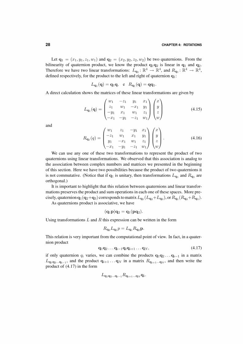
Let q1 = (x1, y1, z1, w1) and q2 = (x2, y2, z2, w2) be two quaternions. From thebilinearity of quaternion product, we know the product q1q2 is linear in q1 and q2.Therefore we have two linear transformations: Lq1 : R4 → R4, and Rq1 : R4 → R4,defined respectively, for the product to the left and right of quaternion q1:

Lq1(q) = q1q, e Rq1(q) = qq1.

A direct calculation shows the matrices of these linear transformations are given by

Lq1(q) =

w1 −z1 y1 x1

z1 w1 −x1 y1

−y1 x1 w1 z1−x1 −y1 −z1 w1

xyzw

(4.15)

and

Rq1(q) =

w1 z1 −y1 x1

−z1 w1 x1 y1

y1 −x1 w1 z1−x1 −y1 −z1 w1

xyzw

. (4.16)

We can use any one of these two transformations to represent the product of twoquaternions using linear transformations. We observed that this association is analog tothe association between complex numbers and matrices we presented in the beginningof this section. Here we have two possibilities because the product of two quaternions itis not commutative. (Notice that if q1 is unitary, then transformations Lq1 and Rq1 areorthogonal.)

It is important to highlight that this relation between quaternions and linear transfor-mations preserves the product and sum operations in each one of these spaces. More pre-cisely, quaternionq1(q2+q3) corresponds to matrixLq1(Lq2+Lq3), orRq1(Rq2+Rq3).

As quaternions product is associative, we have

(q1p)q2 = q1(pq2).

Using transformations L and R this expression can be written in the form

Rq2Lq1p = Lq1Rq2p.

This relation is very important from the computational point of view. In fact, in a quater-nion product

q1q2 . . .qi−1qiqi+1 . . .qN , (4.17)

if only quaternion qi varies, we can combine the products q1q2 . . .qi−1 in a matrixLq1q2...qi−1 , and the product qi+1 . . .qN in a matrix Rqi+1...qN , and then write theproduct of (4.17) in the form

Lq1q2...qi−1Rqi+1...qN qi.

SECTION 8: CONVERTING AMONG REPRESENTATIONS 29

We will now find the matrix inSO(3) corresponding to the rotation defined byϕq(v) =qvq−1. As q is unitary, we have q−1 = q?, and therefore it is proceeded that

ϕq(v) = L(q)R(q?)(v). (4.18)

If q = (x, y, z, w), then q? = (−x,−y,−z, w). Using the matrix of Lq1 in (4.15) withq1 = q and the matrix Rq1 in (4.16) with q1 = q?, and substituting in (4.18), we obtain

L(q)R(q∗) =

w −z y xz w −x y−y x w z−x −y −z w

w −z y −xz w −x −y−y x w −zx y z w

.

Doing the product, we obtain the matrixw2 + x2 − y2 − z2 2xy − 2wz 2xz + 2wy 0

2xy + 2wz w2 − x2 + y2 − z2 2yz − 2wx 02xz − 2wy 2yz + 2wx w2 − x2 − y2 + z2 0

0 0 0 |q|2

. (4.19)

(See exercise 3 for another form of writing this matrix.) As the quaternion q is unitary,we have

|q|2 = w2 + x2 + y2 + z2 = 1.

In Cartesian coordinates the above matrix can be written in the formw2 + x2 − y2 − z2 2xy + 2wz 2xz − 2wy2xy − 2wz w2 − x2 + y2 − z2 2yz + 2wx2xz + 2wy 2yz − 2wx w2 − x2 − y2 + z2

as well as,

2

12 − y

2 − z2 xy + wz xz − wyxy − wz 1

2 − x2 − z2 yz + wx

xz + wy yz − wx 12 − x

2 − y2

.

It is also important to solve the problem of finding the quaternion associated withmatrix L or R. We left this problem for the exercises at the end of the chapter.

8.2 Quaternions and Euler’s angles

Another important relation is to obtain the quaternion associated with a rotation usingEuler’s angles α β and γ. We have three rotations Rx(α), Ry(β), Rz(γ) of angles α, β,γ about axes (1, 0, 0), (0, 1, 0) and (0, 0, 1), respectively. Each one of these rotations isrepresented by ϕqx , ϕqy , and ϕqz , where


qx = cosα

2+ sin

α

2(1, 0, 0),

qy = cosβ

2+ sin

β

2(0, 1, 0),

qz = cosγ

2+ sin

γ

2(0, 0, 1).

The rotation in space is given byRz(γ)Ry(β)Rx(α), and it will be represented by thequaternion q = qzqyqx, obtained from the product of the three quaternions. Supposing

q = w + ix+ jy + kz,

and doing the calculations, we obtain

w = cosα

2cos

β

2sin

γ

2+ sin

α

2sin

β

2sin

γ

2

x = sinα

2cos

β

2cos

γ

2− cos

α

2sin

β

2sin

γ

2

y = cosα

2sin

β

2cos

γ

2+ sin

α

2cos

β

2sin

γ

2

z = cosα

2cos

β

2sin

γ

2+ sin

α

2sin

β

2cos

γ

2.

9 Comments and References

Hamilton’s goal on searching for quaternions consisted on discovering a multiplicationstructure, similar to the one of complex numbers, for the R3 and that could be used torepresent rotations in space. He ended up discovering such structure for the R4. Todayit is known this type of structure exists only in R2, R4 and R8.

Quaternions were introduced in Computer Graphics in the article (Shoemake, 1985).They were already used in the area of Robotics.

For more information about orthogonal transformations of Rn, and in particular, thedemonstration of Euler’s Theorem in its general form, we suggest (Lima, 1999).

9.1 Additional Topics

In this chapter we studied the special group SO(3) of rotations in space which consistsin just a part of the representation of rigid motions in space. The complete group, hasdimension 6 (three degrees of freedom for rotations and three for translations), and iscalled special Euclidean group, denoted by SE(3). An appropriate representation of thisgroup involves the screw theory and the study of the Lie Groups of matrices. Completematerial on these topics can be found in a good textbook in the area of Robotics.

SECTION 10: EXERCISES 31

Quaternions just represent the tip of the iceberg in the study of intrinsic operationsamong geometric objects, a topic covered in the area of Geometric Algebra.

An important topic that we did not cover is the problem of interpolating the n rotationsrepresented by quaternions. From what we covered, this problem is equivalent to the studyof interpolation curves (e.g. Bezier, Splines) in the sphere S3. Several works exist aboutit on the literature. This subject is also very important for the area of GIS (GeographicInformation Systems). The interpolation of rotations using the structure of Lie Groups ofmatrices is an interesting topic. (Alexa, 2002), for instance, describes the interpolationof linear transformations using results from Lie Groups of matrices.

10 Exercises

1. Demonstrate Chasles’ Theorems: ” Every positive rigid motion in R3 can be obtainedby a rotation about a r-axis, followed by a translation along r ” (this type of motion iscalled screw).

2. Describe a method to obtain the quaternion associated with matrix L orR (as definedin this chapter), in homogeneous coordinates.

3. If R : R3 → R3 is a rotation, show that R(u ∧ v) = R(u) ∧R(v).

4. Show there exists no multiplicative structure in R3 among the vectors, similar toquaternions (or to complex numbers). (Suggestion: use the transformation Lq or Rq

defined in the chapter, including the fact that a linear transformation in R3 has 1 realeingenvalue.)

5. If (rij) is a matrix of order 3 representing a rotation in R3, show that the Euler’sangles of the parameterization given by Rz(α)Ry(β)Rz(γ) are determined by:

α = arctg2(√r231 + r232, r33);

β = arctg2(r23

sinβ,r13

sinβ);

γ = arctg2(r32

sinβ,− r31

sinβ),

where arctg2(x, y) is the function arctg(x/y) using the signal of x and y to determinethe quadrant of the resulting angle.

6. Consider the following problem: ” to implement an interactive interface to rotate anobject of R3 about an axis, just using the mouse as input device.” Two solutions exist inthe literature for this problem: the Metaball and the virtual sphere.

a) Describe the model of these two solutions;


b) Compare the solutions and discuss the advantages and disadvantages of each one.

7. Show if a quaternion q commutes with every pure quaternion, then q is real. Usethis fact to show that

ϕq1 = ϕq2 ⇔ q1 = ±q2,

where ϕq is the representation of a rotation defined in (4.9).

8. If p = cos θ + v sin θ is a unit quaternion, and t ∈ R, show that qptq∗ = (qpq∗)t.

9. If q is a unit quaternion, and a, b ∈ R, show that:

qaqb = qa+b e (qa)b = qab.

10. The calculations below show that the product of quaternions is commutative:

pq = exp(log(pq))= exp[log(p) + log(q)]= exp[log(q) + log(p)]= exp(log(q)) exp(log(p)) = qp.

Where is the error?

11. Show that, in the case in which quaternion q is not unitary, the matrix (4.19) of thetransformation ϕq is given by

2|q|2

|q|22 − y

2 − z2 xy + wz xz − wy 0xy − wz |q|2

2 − x2 − z2 yz + wx 0

xz + wy yz − wx |q|22 − x

2 − y2 00 0 0 |q|2

2

.

12. Show thateθu = cos θ + u sin θ,

substituting the expression of θu in the series of potencies of the exponential function

ex =∞∑n=0

xn

n.

13. Let

R =

r11 r12 r13

r21 r22 r23

r31 r32 r33

SECTION 10: EXERCISES 33

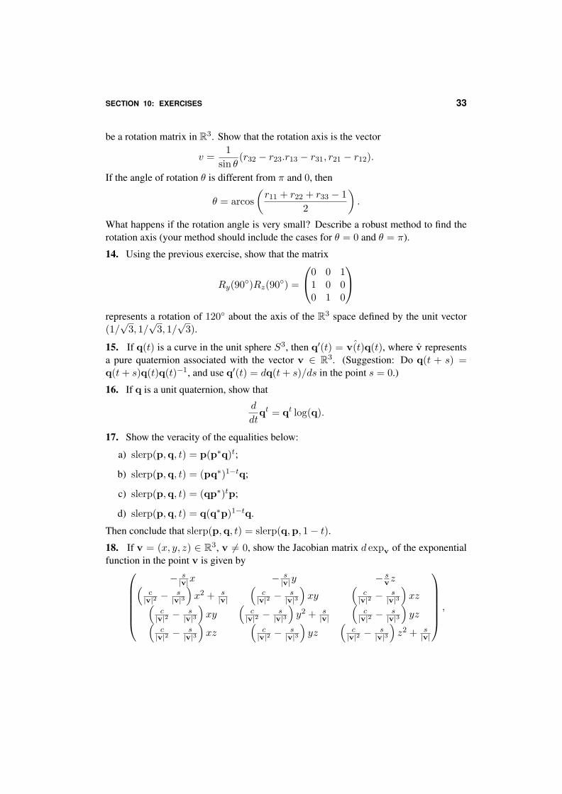
be a rotation matrix in R3. Show that the rotation axis is the vector

v =1

sin θ(r32 − r23.r13 − r31, r21 − r12).

If the angle of rotation θ is different from π and 0, then

θ = arcos(r11 + r22 + r33 − 1

2

).

What happens if the rotation angle is very small? Describe a robust method to find therotation axis (your method should include the cases for θ = 0 and θ = π).

14. Using the previous exercise, show that the matrix

Ry(90◦)Rz(90◦) =

0 0 11 0 00 1 0

represents a rotation of 120◦ about the axis of the R3 space defined by the unit vector(1/√

3, 1/√

3, 1/√

3).

15. If q(t) is a curve in the unit sphere S3, then q′(t) = ˆv(t)q(t), where v representsa pure quaternion associated with the vector v ∈ R3. (Suggestion: Do q(t + s) =q(t+ s)q(t)q(t)−1, and use q′(t) = dq(t+ s)/ds in the point s = 0.)

16. If q is a unit quaternion, show that

d

dtqt = qt log(q).

17. Show the veracity of the equalities below:

a) slerp(p,q, t) = p(p∗q)t;

b) slerp(p,q, t) = (pq∗)1−tq;

c) slerp(p,q, t) = (qp∗)tp;

d) slerp(p,q, t) = q(q∗p)1−tq.

Then conclude that slerp(p,q, t) = slerp(q,p, 1− t).18. If v = (x, y, z) ∈ R3, v 6= 0, show the Jacobian matrix d expv of the exponentialfunction in the point v is given by

− s|v|x − s

|v|y − svz(

c|v|2 −

s|v|3

)x2 + s

|v|

(c|v|2 −

s|v|3

)xy

(c|v|2 −

s|v|3

)xz(

c|v|2 −

s|v|3

)xy

(c|v|2 −

s|v|3

)y2 + s

|v|

(c|v|2 −

s|v|3

)yz(

c|v|2 −

s|v|3

)xz

(c|v|2 −

s|v|3

)yz

(c|v|2 −

s|v|3

)z2 + s

|v|

,


where s = sin |v| and c = cos |v|.

19. Show the Jacobian matrix of the exponential function at the origin v = (0, 0, 0) ∈R3, is given by the matrix

0 0 01 0 00 1 00 0 1

.

(Suggestion: use the expression of the previous exercise for v 6= 0, together with thedefinition of the derivative as a limit.)

20. This exercise shows that the multiplication of two quaternions can be made withonly 8 products instead of 16 products as would be expected. Given two quaterniosq1 = (x1, y1, z1, w1) and q2 = (x2, y2, z2, w2), do

a1 = (x1 − y1)(y2 − z2) a5 = (z1 − x1)(x2 − y2)a2 = (w1 + x1)(w2 + x2) a6 = (z1 + x1)(x2 + y2)a3 = (w1 − x1)(y2 + z2) a7 = (w1 + y1)(w2 − z2)a4 = (z1 + y1)(w2 − x2) a8 = (w1 − y1)(w2 + z2).

Define s = a6 + a7 + a8 and t = (a5 + s)/2. Show that

q1q2 = (a2 + t− s)1 + (a2 + t− s)i + (a3 + t− a8)j + (a4 + t− a7)k.

Bibliography

Alexa, Marc. 2002. Linear Combination of Transformations. ACM Transactions onGraphics, 21(3), 380–387.

Lima, Elon L. 1999. Álgebra Linear. (Terceira edição). Instituto de Matemática Pura eAplicada, Rio de Janeiro: Coleção Matemática Universitária.

Shoemake, K. 1985 (July). Animating Rotation with Quaternion Curve. Pages 245–254of: Computer Graphics (SIGGRAPH ’85 Proceedings), vol. 19.

Índice

Eulerangles of, 7

Euler’s angles, 7and quaternions, 29

geodesic, 21

interpolationgeodesic, 24radial spherical, 24

maximum circle, 21

parameterizationexponential, 22place, 10

quaternions, 4, 14and Euler’s angles, 29and matrices, 27and rotations, 16conjugated, 14

rotationand quaternions, 16Euler’s angles, 7in the space, 4matrix of Euler, 9on the plane, 2quaternions, 4representation by quaternions, 14straight line nodal, 7

35

36 INDEX

yaw, pitch and roll, 8

slerp, 24, 26

yaw, pitch and roll, 8

4 rotations - instituto nacional de matemática pura e...

Documents