4-escwa- vul indexcss.escwa.org.lb/sdpd/3639/pr-s3-4.pdf · socio-ecological systems without...

09/06/2015

1

Economic and Social Commission for Western Asia

Constructing a Vulnerability Index: Impact Chains,

Normalisation and Data Evaluation, Aggregation

and Weighting Methods, Statistical Methods for

Overcoming Data Gaps

Dony El Costa Contributing Expert, Water Resources Section,

Sustainable Development Policies Division,

ESCWA

Regional Workshop on Moving from Climate Change Impact

Assessment to Socio-Economic Vulnerability Assessment in the

Arab Region

Beirut, 8-10 June 2015

Page 2 © Copyright 2015 ESCWA. All rights reserved. No part of this presentation in all its property may be used or reproduced in any form without a written permission

How to Operationalize the IPCC AR 4 (2007)

Definition of Vulnerability

� Exposure refers to changes in climate parameters that might affect socio-ecological

systems.

� Sensitivity tells us about the status quo of the physical and natural environment of

the affected systems that makes them particularly susceptible to climate change.

� Exposure and sensitivity determine the potential impacts of climate change:

focused on the result if climate change took place unrestrictedly, impacting on

socio-ecological systems without further preparation

� Adaptive capacity is ‘‘the ability or potential of a system to respond successfully to

climate variability and change, and includes adjustments in both behaviour and in

resources and technologies’

� Vulnerability is a function of

the character, magnitude, and

rate of climate change and

variation to which a system is

exposed, its sensitivity, and its

adaptive capacity.

09/06/2015

2


How to Operationalize the IPCC AR 4 (2007)

Definition of Vulnerability

• Vulnerability is ‘‘the degree to which a system is susceptible to, and unable

to cope with, adverse effects of climate change, including climate

variability and extremes. Vulnerability is a function of the character,

magnitude, and rate of climate change and variation to which a system is

exposed, its sensitivity, and its adaptive capacity’’ (McCarthy et al., 2001; IPCC AR3,

2001)

� the defining

concepts

themselves are

vague and difficult

to make

operational

� lack of clarity on

how to combine

the defining

concepts

Hinkel (2011)


Recommended Steps for Constructing a

Composite Indicator

• Definition: A composite indicator is formed when individual indicators are

compiled into a single index, on the basis of an underlying model of the

multi-dimensional concept that is being measured. (OECD Glossary of

statistics)

� Step 1. Defining the phenomenon/ Developing a theoretical framework/ Conceptualizing the Composition and Structure

� Step 2. Selecting indicators� Step 3. Data pre-processing� Step 4. Normalisation of data� Step 5. Multivariate analysis/

Statistical Coherence� Step 6. Weighting and aggregation� Step 7. Robustness/ sensitivity/

Uncertainty analysis� Step 8. Back to the details

(indicators)� Step 9. Presentation and

dissemination

Theoretical

Methodological

/ Statistical

Index construction

flowchart

OECD (2008)Tate (2013)

09/06/2015

3


Composite Indicators: Pros and Cons

Pros Cons

� Can summarise complex, multi-dimensional realities with a view to supporting decision makers.

� Are easier to interpret than a battery of many separate indicators.

� Can assess progress of countries over time.

� Reduce the visible size of a set of indicators without dropping the underlying information base.

� Thus make it possible to include more information within the existing size limit.

� Place issues of country performance and progress at the centre of the policy arena.

� Facilitate communication with general public (i.e., citizens, media, etc.) and promote accountability.

� Help to construct/underpin narratives for lay and literate audiences.

� Enable users to compare complex dimensions effectively.

� May send misleading policy messages if poorly constructed or misinterpreted.

� May invite simplistic policy conclusions.

� May be misused, e.g., to support a desired policy, if the construction process is not transparent and/or lacks sound statistical or conceptual principles.

� The selection of indicators and weights could be the subject of political dispute.

� May disguise serious failings in some dimensions and increase the difficulty of identifying proper remedial action, if the construction process is not transparent.

� May lead to inappropriate policies if dimensions of performance that are difficult to measure are ignored.


RICCAR Vulnerability Assessment Nested Structure –

Sector/ Sub-sector/ Climate Change Impact

Thematic Clustering/

Theoretically derived

categorization of

indicators into

components,

dimensions, pillars

09/06/2015

4


Identifying Indicators from Impact Chains

� Developed to identify indicators in order to operationalise the vulnerability assessment for

each climate change impact

� outlines for each of the three components the key factors contributing to the vulnerability

� allows a better understanding of the cause-effect relationship between climate change and

its implications for a selected system

”Impact chain for “Change in

water availability


Normalisation and Evaluation of Data

� We deal with data of different scales of measurement (metric, ordinal, nominal), different value ranges and different units

� For metric data:� Different nature of indicators (positive vs. negative orientation towards the index)

� Asymmetric distribution, different variances, ranges of variation, and outliers

� data first need to be transformed into a unit-less score on a common scale, before aggregation

� For the integrated assessment of vulnerability in the Arab region:

� For the Exposure and Sensitivity components: a scale with a value range of 1 to 10 is applied, with the value 1 representing a low vulnerability and the value 10 representing a high vulnerability

� For the Adaptive Capacity Indicators: the value 1 represents a low adaptive capacity (high vulnerability) and the value 10 represents a high adaptive capacity (low vulnerability)

� Depending on the type of data, different techniques can be applied:� Min-Max Normalisation

� Evaluation of Indicators Using a Reference

� Evaluating Indicators Based on Expert Opinion

09/06/2015

5


Normalisation and Evaluation of Metric Data:

Min-Max Normalisation

Road density, Xi

(1)

Data Log-

transformed

Ln(Xi)

(2)

Normalised

values

(Ln(Xi)-(-0.7))/

(6.3–(-0.7))

(3)

Classes

(4)

Algeria 4.8 1.6 0.33 4

Bahrain 545.7 6.3 1.00 10

Djibouti 47.3 3.9 0.65 7

Egypt 13.2 2.6 0.47 5

Iraq 13.7 2.6 0.48 5

Jordan 9.6 2.3 0.43 5

Kuwait 8.1 2.1 0.40 5

Lebanon 39.3 3.7 0.63 7

Libya 66.7 4.2 0.70 8

Mauritania 4.7 1.6 0.33 4

Morocco 1.1 0.1 0.12 2

Palestine 13.1 2.6 0.47 5

Oman 77.8 4.4 0.72 8

Qatar 77.8 4.4 0.72 8

Saudi Arabia 78.6 4.4 0.73 8

Somalia 10.3 2.3 0.44 5

Sudan

(including South Sudan)3.5 1.2 0.28 3

Syrian Arab Republic 0.5 -0.7 0.00 1

Tunisia 37.7 3.6 0.62 7

United Arab Emirates 11.9 2.5 0.46 5

Yemen 4.9 1.6 0.33 4

• Indicator: Road density

• log-transformation

• In the Arab Countries, the

original values range from

0.5 km of road per 100

km2 of land area, to 545.7

km of road per 100 km2 of

land area.


Normalisation of data: overview of some methods for

metric data

Method Equation

1. Ranking )x(RankIt

qc

t

qc=

2. Standardization (or z-scores)

t

cqc

t

cqc

t

qct

qc

xxI

=

=−

=

σ

3. Re-scaling

)x(min)x(max

)x(minxI

00

0

t

qc

t

qc

t

qc

t

qct

qc

−

−

= .

4. Distance to reference country

0t

cqc

t

qct

qc

x

xI

=

= or 0

0

t

cqc

t

cqc

t

qct

qc

x

xxI

=

=−

=

5. Logarithmic transformation )xln(I t

qc

t

qc=

6. Categorical scales

...

60yx

80yx

100yx

t

qc

t

qc

t

qc

t

qc

t

qc

t

qc

else then percentile th- 35upperthe in if

else then percentile th-15 upperthe in if

else then percentile th-5 upperthe in if

=

=

=

OECD/JRC 2008

Normalisation Methods:

� Linear scales

� Ordinal scales

� Ratio scales

09/06/2015

6


Normalisation of data: overview of some

methods

7. Indicators above or below the mean

0Ip)1(xx)p1(

1Ip)1(xx

1Ip)1(xx

t

qc

t

cqc

t

qc

t

qc

t

cqc

t

qc

t

qc

t

cqc

t

qc

0

0

0

=+<<−

−=−<

=+>

=

=

=

then if

then if

then if

8. Cyclical indicators (OECD) ( )( )( )t

qct

t

qct

t

qct

t

qct

qc

xExE

xExI

−

−

=

9. Balance of opinions (EC) ( )∑

−

−=

eN

e

1t

qc

t

qce

e

t

qc xxsgnN

100I

10. Percentage of annual differences over consecutive years

t

qc

1t

qc

t

qct

qcx

xxI

−

−

=

Pro: simple, no outliers

Cons: p arbitrary, no absolute levels

Pro: minimize cycles

Cons: penalize irregular indic.

Pro: based on opinions

Cons: no absolute levels

Pro: no levels but changes

Cons: low levels are equal to high levelsOECD/JRC (2008)


Normalisation and Evaluation of Data: Evaluation

of Indicators Using a Reference

� Some data sets cannot be normalised in such a standardised way as this would not

adequately represent the meaning of an indicator value in regard to the relevant vulnerability

component.

� This meaning – again on a scale from 1 to 10 – needs to be assigned to each indicator value:

evaluation. For that purpose, a reference such as an existing and widely accepted index can

be used to allocate the indicator values into classes.

� Practical example:

� For the indicator Total Available Renewable Water Resources (TARWR) per capita the classes

to indicate the level of sensitivity could be based on the Falkenmark Indicator. The

Falkenmark Indicator proposes a threshold of 1,700m3 of available water resources per capita

per year for water stressed and 1000m3 per capita per year for water scarce-countries.

Falkenmark Index (m3 per capita) Value range TARWR

(m3 per capita)

Sensitivity Class

>1.700 – No stress n.a. 1 – low sensitivity

n.a. 2

n.a. 3

n.a. 4

>1.000 – 1.700 - Stress 1500 – 1750 5

1250 – 1500 6

>1000 – 1250 7

500 – 1.000 Scarcity 750 – 1000 8

500 – 750 9

< 500 – Absolute scarcity 0 – <500 10 – high sensitivity

09/06/2015

7


Normalisation and Evaluation of Data: Evaluating

Indicators Based on Expert Opinion

� when references or thresholds are not available

� Example in the context of the integrated vulnerability assessment of the Arab region: land use land cover “evaluation”, with the experts of the VA-WG. The experts evaluated the different classes of the Global Land Cover-SHARE data set, assigning the different classes provided in the data to the scale of ten

Sensitivity value / classGlobal Land Cover-SHARE

Identification NumberDescription

2 1 Artificial Surfaces

8 2 Cropland

5 3 Grassland

8 4 Tree Covered Areas

7 5 Shrubs Covered Areas

8 6 Herbaceous vegetation aquatic or regularly flooded)

5 7 Mangroves

5 8 Sparse vegetation

1 9 Baresoil

n.a 10 Snow and glaciers*

9 11 Water bodies

* The description for “snow and glaciers” in Gobal Land Cover-SHARE refers to permanent snow cover and glaciers. It was thus determined to be not applicable (n.a.) for the Arab region.


Metric Data Normalisation and Evaluation: Some

Practical Guidelines1) Data representation/ Transformation into non-dimensional scales: percentages, per capita, density functions

� percentage of elderly or the elderly count? Unemployment rates or the number of unemployed? Population counts or population densities?

� Two main representational methods are available: � 'absolute representations,‘ which use the variable counts; and � ‘relative composition‘ methods, where relative numbers are

computed so as to consider relative proportions of vulnerable populations� using absolute size greatly influenced by the ranks of total

population� absolute composition might be used if the purpose of the

index is to identify the number of vulnerable people, such as for evacuation planning

� combining both absolute and relative representations of variables, through averaging the absolute and relative normalised values, is possible

� don’t only relate to demographic-related indicators, but also most socio-economic and in some instances environmental indicators: � should we use the total amount of official development aid, the

official development aid per capita, or official development aid as percentage of government revenues?

� Should we use the number of scientific and technical journal articles or express this number per million population?

� Should we use the number of hospital beds or express this number per thousand population?

09/06/2015

8



Practical Guidelines

2) A statistical analysis of the original raw data is essential as it enables: � the identification of outliers

� Indicative of heavy tailed distribution, a mixture of two distributions, or errors

� distort the correlation structure and � become unintended benchmarks during normalization

� Particularly problematic in the case of min-max linear transformation

� Techniques to identify outliers: � Percentile rank� Skewness and kurtosis rule of thumb� Boxplot analyses� Leverage and influence analyses

� Need for scale transformation?� Imputation of missing values




� Missing values : imputation necessary to obtain a complete dataset� Case deletion/ Indicator deletion?

� Approaches:� introduce more than one indicator per pillar/ dimension/

component to complement each other

� data from the most recent year available: threshold?

� Hot-deck imputation/ Cold-deck imputation

� Unconditional sample mean/median/mode

� Regression imputation

� Imputation with MAR and MCAR assumptions� Expectation maximization

� Markov Chain Monte Carlo (MCMC) multiple imputation

� Measure the reliability of imputed values: sensitivity analysis

09/06/2015

9




3) Minimum and Maximum values choices

�Main considerations:� Closely linked to/ dependent on the outliers treatment step� Using regional or global minima and maxima?

� Is there a potential for the countries of the region with the highest scores to continue their progress on some indicators?

� Might well be the case for some indicators of the adaptive capacity dimension: technology indicators? governance indicators? educational attainment indicators?

� From a time series perspective� Panel normalisation/ annual normalisation� Fixed min and max values recommended: preserve the

rescaling factor and make the transformation stable through time




4) classification decisions for metric data:

� choice depends on data distribution:

� equal intervals classification;

� quantile classification;

� natural breaks (Jenks) classification;

� user defined classification;

� geometrical intervals classification;

� mean-standard deviation method;

� nested means method;

� maximum breaks classification

�most used: equal intervals classification, the quantiles classification,

and the user defined

09/06/2015

10



Practical Guidelines5) Directionality change/ data inversion: several approaches/ several levels:

� At the indicator level: different indicators have different directions of functional relationship with the construct being measured, compare:� a temperature increase and an increase in precipitation (Sensitivity

component)� Literacy rates, GDP/capita and refugees in percent of population,

disability prevalence data (Adaptive capacity component)� Data inversion during the normalisation phase necessary for the

indicators class numbers to indicate similar vulnerability states � Can be handled within the normalisation procedure for single

indicators: example of a (0-1) min-max re-scaling,

vs

� Inversion after the normalization and classification step: apply the (11-x) transformation




� data inversion: necessary at (almost) every aggregation level to take advantage of the partial compensability property of the geometric aggregation, � Low (high) values should indicate high (low) vulnerability states� This is in contrast to the classification convention of exposure and

sensitivity indicators

� The following equivalences/ correspondences should be kept in mind:� Low adaptive capacity - High Exposure/ Sensitivity - High

Vulnerability� High adaptive capacity - Low Exposure/ Sensitivity - Low

Vulnerability

� Similarly inversion is necessary � When combining Sub-sectors vulnerability indices into Sectoral

indices� When combining Sectoral vulnerability indices into an Overall

vulnerability index

09/06/2015

11


Aggregation Methods: The Linear Additive

Aggregation and the Arithmetic Aggregation

� There is a large variety of different aggregation techniques: compensatory and non-compensatory

� Additive aggregation is a weighted (or unweighted) linear combination of the normalized indicators.

� A special case is an arithmetic aggregation

Index value = ∑ wiX

i = (w

1 * X

1+ w

2 * X

2+ w

3 * X

3+ � + w

n * X

n)

n= number of indicatorsw

i= weight for indicator i, with 0 ≤ w

i ≤ 1 and ∑ w

i = 1

Xi= normalised value of indicator i

� main drawbacks in the context of in socio-economic vulnerability assessments � the preference independence condition, or the mutually preferential

independence of the different indicators, dimensions, or components: property of “no interaction“ can be problematic

� the property of full compensability� violates preferred invariance property to plausible transformations


Aggregation Methods: Geometric Aggregation

� The geometric aggregation, a nonlinear aggregation technique,

avoids these issues with interaction and compensability. It is the

product of normalized weighted (or unweighted) indicators and can be

calculated using the following formula:

Index value = π Xiwi= (X1)

w1 * (X2)

w2* (X3)

w3 *

�* (Xn)

wn

Where,

n= number of indicators

wi= weight for indicator i, with 0 ≤ wi ≤ 1 and ∑ wi = 1

Xi = normalised value of indicator i

� It has the property of partial compensability, meaning that a poor

performance in some indicators cannot be easily compensated for by

high values in other indicators

� countries with divergent normalized indicators are penalised

Intuition behind

Partial/ Full

compensability:

Arithmetic average of

1 and 9= (1+9)/2 = 5

Geometric average of

1 and 9= (1*9) 1/2 = 3

09/06/2015

12


Aggregation method in the Integrated

Vulnerability Assessment of the Arab Region

� For the integrated vulnerability assessment of the Arab region, a geometric aggregation approach was chosen. As previously noted, depending on the knowledge available, it can be used with or without assigned weights.

� There are several levels on which aggregation will be done in order to implement the integrated vulnerability assessment methodology.

� The aggregation methodology consists of a multi-level (nested) structure which incorporates three main architectural elements: components, dimensions, and indicators:� The three components are exposure, sensitivity, and adaptive capacity.� Exposure and sensitivity are aggregated to obtain an index for potential

impact, which is then combined with adaptive capacity to obtain a vulnerability index.

� The sensitivity and adaptive capacity components are further composed of several dimensions.

� Each dimension is in turn represented by several indicators.� This general structure can be simplified or elaborated upon according to the

theoretical and conceptual framework, and the specificities of the index design structure


RICCAR Vulnerability Assessment Nested Structure –

Sector/ Sub-sector/ Climate Change Impact

09/06/2015

13


Aggregation approach for the Adaptive Capacity

component

* Individual indicators are aggregated to obtain sub-indices. ** Individual indicators and sub-indices are aggregated to obtain an index for every dimension.*** The six dimensions are aggregated to calculate an index for the Adaptive capacity component.


Aggregation approach to the Infrastructure

dimension

The Infrastructure dimension aggregates eleven indicators that relate to five

pillars: energy, transport, health, water and sanitation supply, and environment.

09/06/2015

14


Weighting Methods

� Weighting schemes can have a significant effect on countries' vulnerability scores

� Can be assigned to 1) the indicators of each dimension; 2) the dimensions of each component; and 3) the three components of vulnerability.

� Statistical methods:� Advantages� Drawbacks

� Participatory methods, examples:� budget allocation process (BAP)� analytic hierarchy process (AHP): produces coherent and robust weights

based on a set of stated preferences of experts from rotating pair-wise comparison of priorities, and controls for internal consistency for priority assessment.

� When the relative importance of indicators is judged to be the roughly the same, or when to the trade-offs between indicators or dimensions are poorly understood so that the assignment of differential weights cannot be justified, equal weightings might be applied.

� Remarks regarding the use of equal weightings� distinction between the “targeted” or “ex ante”, and the “ex-post”

importance,


Introduction of weights

CIDimension i = (SE1 * SE3 *: * SEn)1/n

CIWeighted Dimension i = (SE1) w1 * (SE2)

w2 * (SE3) w3 * : * (SEn)

wn

CI Dimension i = (AC1 * Sub-Ind AC2 * AC3 * : * ACn)1/n

:

CI weighted Dimension i = AC1w1 * (Sub-IndAC2)

wSub-IndAC2 * AC3w3* : * ACn

wn

CI Adaptive Capacity= (CIDim1 * CIDim2 * CIDim3 * CIDim4 * CIDim5 * CIDim6)1/6

CI Weighted Adaptive Capacity =

(CIDim1)wDim1 * (CIDim2)

wDim2 * (CIDim3)wDim3 * (CIDim4)

wDim4 * (CIDim5)wDim5 *

(CIDim6)wDim6

09/06/2015

15


Aggregating the Components of Vulnerability

Vx = (PIx * ACx)1/2

or

Vx = (PIx)wPI * (ACx)

wAC

PIx = (EXx * SEx)1/2

or

PI Weighted = (EXx)wEX

* (SEx)wSE


Impacts of choices of operationalisation of the

IPCC AR4 (2007)

Definition 1: Sensitivity, exposure, and adaptive capacity are assumed to have an equal influence on vulnerability, Vx = ( EXx * SEx * ACx)

1/3

Since the potential impact is calculated by:(EXx * SEx)

1/2 = PIxVulnerability can also be calculated using the following formula:

Vx=(PIx2 * ACx)

1/3 = PIx2/3 * ACx

1/3

Definition 2: Potential impact and adaptive capacity have an equal influence on vulnerability, where Potential Impact is itself equally influenced by exposure and sensitivity.

In this case, Vx = (PIx * ACx)

1/2= PIx

1/2 * ACx

1/2

Hence, in this case wPI = wAC = ½.

09/06/2015

16


Overview of inversion and aggregation steps

towards the overall vulnerability

Component

(C)

Original Indicator Values:

EX + SE: high values =

high V

AC: mixed assessment1

Inverse Indicato

rs2

Aggregation to

vulnerability

components

Aggregation to PI

Output PI + AC

Aggregation to

V single

Output V single

Aggregation to V total

Output V total

EX EX-1 Inv EX-1

Geometric aggregation � InvEXC

(InvEXC * InvSEC)½ �PI_Inv

Inv (PI_Inv) � PI

Interpretation 1:

(InvPI * InvPI * AC)1/3 �InvV

Inv (InvV) � V single

(InvVA * InvVB) ½ �Inv V total

Inv (Inv V total)� V total

EX-2 Inv EX-2

EX-3 Inv EX-3

EX-x Inv E-xx

SE SE-1 Inv SE-1 Geometric aggregation � InvSEC

SE-2 Inv SE-2

SE-3 Inv SE-3Interpretation 2:

(InvPI * AC)1/2�InvV

Inv (InvV) � V single

(InvVA * InvVB) ½ �Inv V total

Inv (Inv V total)� V totalSE-x

AC AC-1Geometric aggregation � AC

� ACAC-2 Inv AC-2

AC-3

AC-x Inv AC-4

Notes:1 The inversion will only be necessary for those adaptive capacity indicators where high values represent high vulnerability, e.g., refugees or people with disability figures.2”Inv” refers to the inversion of the direction of some indicators or components through the 11 –x transformation, see Part I: Chapter 7.3.


Aggregating Vulnerability within Sectors

Sub-sector vulnerabilities can be aggregated to a sectoral vulnerability

using the geometric approach by applying the following formula:

VSector = (V1 * V2 * : * Vn)1/n

For example, in the sector Ecosystems and Biodiversity, the vulnerability

towards the climate change impacts ‘change in water availability on wetlands’

and ‘change in water availability on forests’ is assessed.

09/06/2015

17


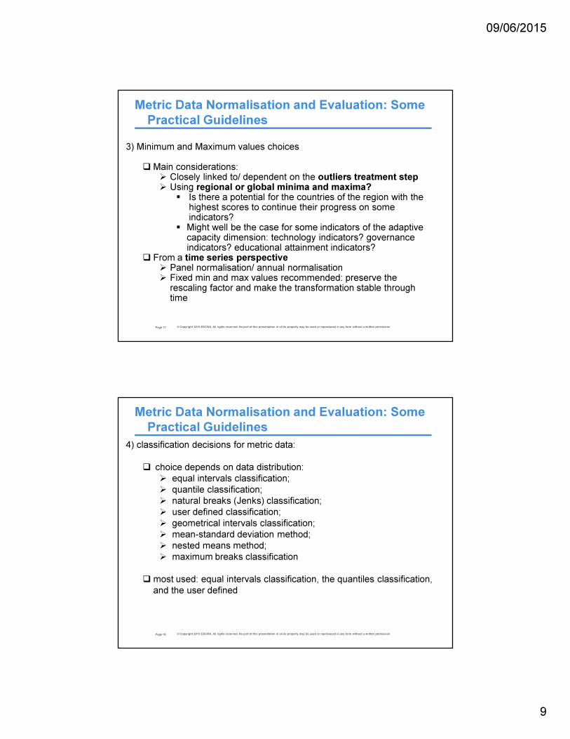
Aggregating Sectoral Vulnerabilities to Overall

Vulnerability

� The overall vulnerability of the Arab region –comprises several sectors.

� an aggregation of sectoralvulnerabilities is problematic when the vulnerability of one sector is in a direct cause-effect relationship with another sector

� We recommend aggregating only the sectoral vulnerabilities highlighted in the figure using the following formula: V

overall= (V

1 *V

2 *V

3)1/3

Economic and Social Commission for Western Asia

THANK YOU

Dony El Costa

Water Resources Section, Sustainable

Development Policies Division, ESCWA

[email protected];

[email protected]

4-escwa- vul indexcss.escwa.org.lb/sdpd/3639/pr-s3-4.pdf · socio-ecological systems without...

Documents