4–1

4 Coherence Selection: Phase Cycling and Gradient Pulses

A multiple-pulse NMR experiment is designed to manipulate the spins in a certain carefully defined way so as to produce a particular spectrum. However, a given pulse sequence usually can affect the spins in several different ways and as a result the final spectrum may contain resonances other than those intended when the experiment was designed. The presence of such resonances may result in extra crowding in the spectrum, they may obscure the wanted peaks and they may also lead to ambiguities of interpretation. It is thus all but essential to ensure that the responses seen in the spectrum are just those we intended to generate when the pulse sequence was designed. There are two principle ways in which this selection of required signals is achieved in practice. The first is the procedure known as phase cycling. In this the multiple-pulse experiment is repeated a number of times and for each repetition the phases of the radiofrequency pulses are varied through a carefully designed sequence. The free induction decays resulting from each repetition are then combined in such a way that the desired signals add up and the undesired signals cancel. The second procedure employs field gradient pulses. Such pulses are short periods during which the magnetic field is made deliberately inhomogeneous. During a gradient pulse, therefore, any coherences present dephase are apparently lost. However, the application of a subsequent pulsed field gradient can undo this dephasing and cause some of the coherences to refocus. By a careful choice of the gradient pulses within a pulse sequence it is possible to ensure that only the coherences giving rise to the wanted signals are refocused. Historically, in the development of multiple-pulse NMR, phase cycling has been the principle method used for selecting the desired outcome. Pulsed field gradients, although their utility had been known from the earliest days of NMR, have only relatively recently been seen as a practical alternative. Both methods can be described using the key concept of coherence order and by utilising the idea of a coherence transfer pathway. In this lecture we will start out by describing phase cycling, emphasising first its relation to the idea of difference spectroscopy and then moving on to describe the formal methods for writing and analysing phase cycles. The tools needed to describe selection with gradient pulses are quite similar to those used in phase cycling, and this will enable us to make rapid progress through this topic. There are, however, some key differences between the two methods, especially in regard to the sensitivity and other aspects of multi-dimensional NMR experiments.

4.2.1 Phase

In the simple vector picture of NMR the phase of a radiofrequency pulse determines the axis along which the magnetic field, B1, caused by the

4–2

oscillating radiofrequency current in the coil, appears. Viewed in the usual rotating frame (rotating at the frequency of the transmitter) this magnetic field is static and so it is simple to imagine its phase as the angle, β, between a reference axis and the vector representing B1. There is nothing to indicate which direction ought to be labelled x or y; all we know is that these directions are perpendicular to the static field and perpendicular to one another. So, provided we are consistent, we are free to decide arbitrarily where to put this reference axis. In common with most of the NMR community we will decide that the reference axis is along the x-axis of the rotating frame and that the phase of the pulse will be measured from x; thus a pulse with phase x has a phase angle, β, of zero. Similarly a pulse of phase y has a phase angle of 90° or π/2 radians. Modern spectrometers allow the phase of the pulse to be set to any desired value. The NMR signal, that is the free induction decay (FID), is recorded by measuring the voltage generated in a coil as it is cut by precessing transverse magnetization. Most spectrometers take this high-frequency signal and convert it to the audio-frequency range by subtracting a fixed reference frequency. Almost always this fixed reference frequency is the same as the transmitter frequency and the effect of this choice is to make it appear that the FID has been detected in the rotating frame. Thus the frequencies which appear in the detected FID are the offset or difference frequencies between the Larmor frequency and the rotating frame frequency. Like the pulse, the NMR receiver also has associated with it a phase. If we imagine at time zero that there is transverse magnetization along the x-axis (of the laboratory frame) and that a small coil is wound around the x-axis the voltage induced in the coil as the magnetization precesses is proportional to the x-component i.e. proportional to cos(ω0t). On the other hand, if the magnetization starts out along the –y axis the induced voltage is proportional to sin(ω0t), simply as this is the projection onto the x-axis as the magnetization vector rotates in the transverse plane. In mathematical terms the detected signal can be always be written cos(ω0t + φ), where φ is a phase angle. The magnetization starting out along x gives a signal with phase angle zero, whereas that starting along –y has a phase angle of –π/2. The NMR receiver can differentiate between the cosine and sine modulated parts of the signals by using two detectors fed with reference signals which are shifted in phase by 90° relative to one another. The detection process involves using a device called a mixer which essentially multiplies together (in an analogue circuit) the incoming and reference signals. The inputs to the mixers at the reference frequency, ωref, take the form of a cosine and a sine for the two detectors, as these signals have the required 90° phase shift between them. If the incoming signal is cos(ω0t + φ) the outputs of the two mixers are

( ) ( ) ( )[ ]( ) ( ) ( )[ ]

0

90

12

12

° + = + + + +

° + = + + − +

: cos cos cos cos –

: cos sin sin sin –

ω φ ω ω φ ω ω φ ω

ω φ ω ω φ ω ω φ ω

0 ref 0 ref 0 ref

0 ref 0 ref 0 ref

t t t t

t t t t

These outputs are filtered to remove the high frequency components (the first terms on the right) and the outputs from the 0° and 90° detectors

4–3

become the real and imaginary parts of a complex number. If we add a damping term and ignore the numerical factors, the detected (complex) signal is

( ) ( )[ ]( )( )

cos – sin – exp( )

exp – exp( ) exp( )

ω φ ω ω φ ω

ω ω φ

0 ref 0 ref

0 ref

i

- i i

+ − + −

≡ − −

t t Rt

t Rt

Fourier transformation of this signal gives a peak at the offset frequency, ω0 – ωref, and with phase φ. If φ is zero, then an absorption mode peak is expected, whereas if φ is π/2 a dispersion mode peak is expected; in general a line of mixed phase is seen. The detector system is thus able to determine not only the frequency at which the magnetization is precessing, but also its phase i.e. its position at time zero. In the above example the two reference signals sent to the two detectors were chosen deliberately so that magnetization with phase φ = 0 would result in an absorption mode signal. However, we could alter the phase of these reference signals to produce any phase we liked in the spectrum. If the reference signals were cos(ωreft + β) and sin(ωreft + β) the FID would be of the form

( ) ( )[ ]( )( )

cos – sin – exp( )

exp – exp( ( )) exp( )

ω φ ω β ω φ ω β

ω ω φ β

0 ref 0 ref

0 ref

i

- i i

+ − − + − −

≡ − − −

t t Rt

t Rt

Now we see that the line has phase (φ - β). The key point to note that as β is under our control we can alter the phase of the lines in the spectrum simply by altering the reference phase to the detector.

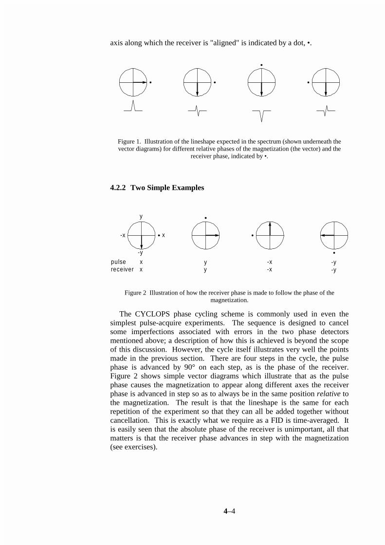
In modern NMR spectrometers the phase, β, of this reference is under the control of the pulse programmer. This receiver phase and the ability to alter it freely is a key part of phase cycling. The usual language in which the receiver phase is specified is to talk about "the receiver being aligned along x", by which it is meant that the receiver phase is set to a value such that if, at the start of the FID, there were solely magnetization along x the resulting spectrum would contain an absorption mode signal. Likewise, "aligning the receiver along –y" means that an absorption mode spectrum would result if the magnetization were solely along –y at the start of the FID. If the magnetization were aligned along x instead, such a receiver phase would result in a dispersion mode spectrum (β = π/2). Of course in practice we can always phase the spectrum to produce whatever lineshape we like, regardless of the setting of the receiver phase. Indeed the process of phasing the spectrum and altering the receiver phase are the same. However, as signals are often combined before Fourier transformation and phasing, the relative phase shifts that can be obtained by altering the receiver phase are important. Figure 1 shows, using the vector model, the relationship between the position of magnetization at the start of the FID, the receiver phase and the phase of the lineshape in the corresponding spectrum. In this diagram the

4–4

axis along which the receiver is "aligned" is indicated by a dot, •.

Figure 1. Illustration of the lineshape expected in the spectrum (shown underneath the vector diagrams) for different relative phases of the magnetization (the vector) and the

receiver phase, indicated by •.

4.2.2 Two Simple Examples

x

y

-x

-y

pulsereceiver

xx

yy

-x-x

-y-y

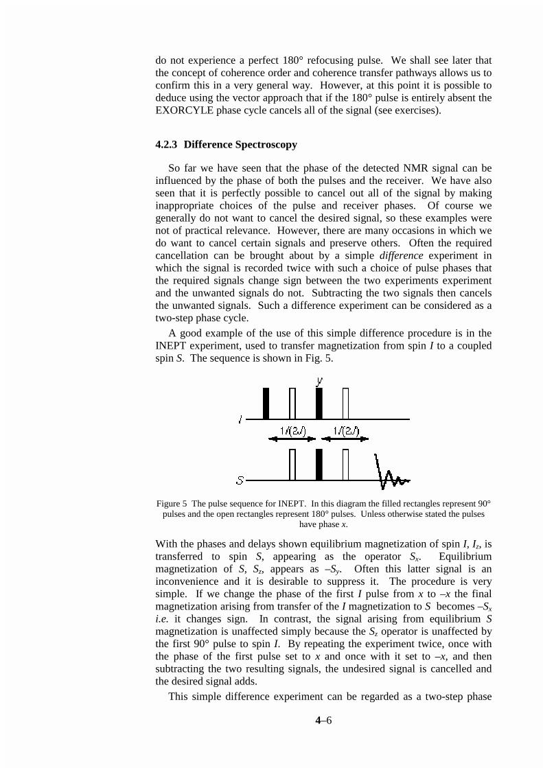
Figure 2 Illustration of how the receiver phase is made to follow the phase of the magnetization.

The CYCLOPS phase cycling scheme is commonly used in even the simplest pulse-acquire experiments. The sequence is designed to cancel some imperfections associated with errors in the two phase detectors mentioned above; a description of how this is achieved is beyond the scope of this discussion. However, the cycle itself illustrates very well the points made in the previous section. There are four steps in the cycle, the pulse phase is advanced by 90° on each step, as is the phase of the receiver. Figure 2 shows simple vector diagrams which illustrate that as the pulse phase causes the magnetization to appear along different axes the receiver phase is advanced in step so as to always be in the same position relative to the magnetization. The result is that the lineshape is the same for each repetition of the experiment so that they can all be added together without cancellation. This is exactly what we require as a FID is time-averaged. It is easily seen that the absolute phase of the receiver is unimportant, all that matters is that the receiver phase advances in step with the magnetization (see exercises).

4–5

x

y

-x

-y

Figure 3. Illustration of how failing to move the receiver phase in concert with the phase of the magnetization leads to signal cancellation; the sum of the spectra shown is zero.

Finally, Fig. 3 shows the result of "forgetting" to move the receiver phase; if the signals from all four steps are added together the signal cancels completely. Similar cancellation arises if the receiver phase is moved backwards i.e. x, –y, –x, y rather than x, y, –x, –y (see exercises).

Figure 4. The effect of altering the phase of the 180° pulse in a spin echo.

A second familiar phase cycle is EXORCYLE which is used in conjunction with 180° pulses used in spin echoes. Figure 4 shows a simple vector diagram which illustrates the effect on the final position of the vector when the phase of the 180° pulse is altered through the sequence x, y, –x, –y. It is seen that the magnetization refocuses along the y, –y, y and –y axes respectively as the 180° pulse goes through its sequence of phases. If the four signals were simply added together in the course of time averaging they would completely cancel one another. However, if the receiver phase is adjusted to follow the position of the refocused magnetization, i.e. to take the values y, –y, y, –y, each repetition will give the same lineshape and so the signals will add up. This is the EXORCYCLE sequence. As before, it does not matter if the receiver is actually aligned along the direction in which the magnetization refocuses, all that matters is that when the magnetization shifts by 180° the receiver should also shift by 180°. Thus the receiver phase could just as well have followed the sequence x, –x, x, –x. For brevity, and because of the way in which these phase cycles are encoded on spectrometers, it is usual to refer to the pulse and receiver phases using numbers with 0, 1, 2, 3 representing phases of 0°, 90°, 180° and 270° respectively (that is alignment with the x, y, –x and –y axes). So, the phases for EXORCYCLE can be written as 0 1 2 3 for the 180° pulse and 0 2 0 2 for the receiver. The EXORCYCLE sequence is designed to eliminate those signals which

4–6

do not experience a perfect 180° refocusing pulse. We shall see later that the concept of coherence order and coherence transfer pathways allows us to confirm this in a very general way. However, at this point it is possible to deduce using the vector approach that if the 180° pulse is entirely absent the EXORCYLE phase cycle cancels all of the signal (see exercises).

4.2.3 Difference Spectroscopy

So far we have seen that the phase of the detected NMR signal can be influenced by the phase of both the pulses and the receiver. We have also seen that it is perfectly possible to cancel out all of the signal by making inappropriate choices of the pulse and receiver phases. Of course we generally do not want to cancel the desired signal, so these examples were not of practical relevance. However, there are many occasions in which we do want to cancel certain signals and preserve others. Often the required cancellation can be brought about by a simple difference experiment in which the signal is recorded twice with such a choice of pulse phases that the required signals change sign between the two experiments experiment and the unwanted signals do not. Subtracting the two signals then cancels the unwanted signals. Such a difference experiment can be considered as a two-step phase cycle. A good example of the use of this simple difference procedure is in the INEPT experiment, used to transfer magnetization from spin I to a coupled spin S. The sequence is shown in Fig. 5.

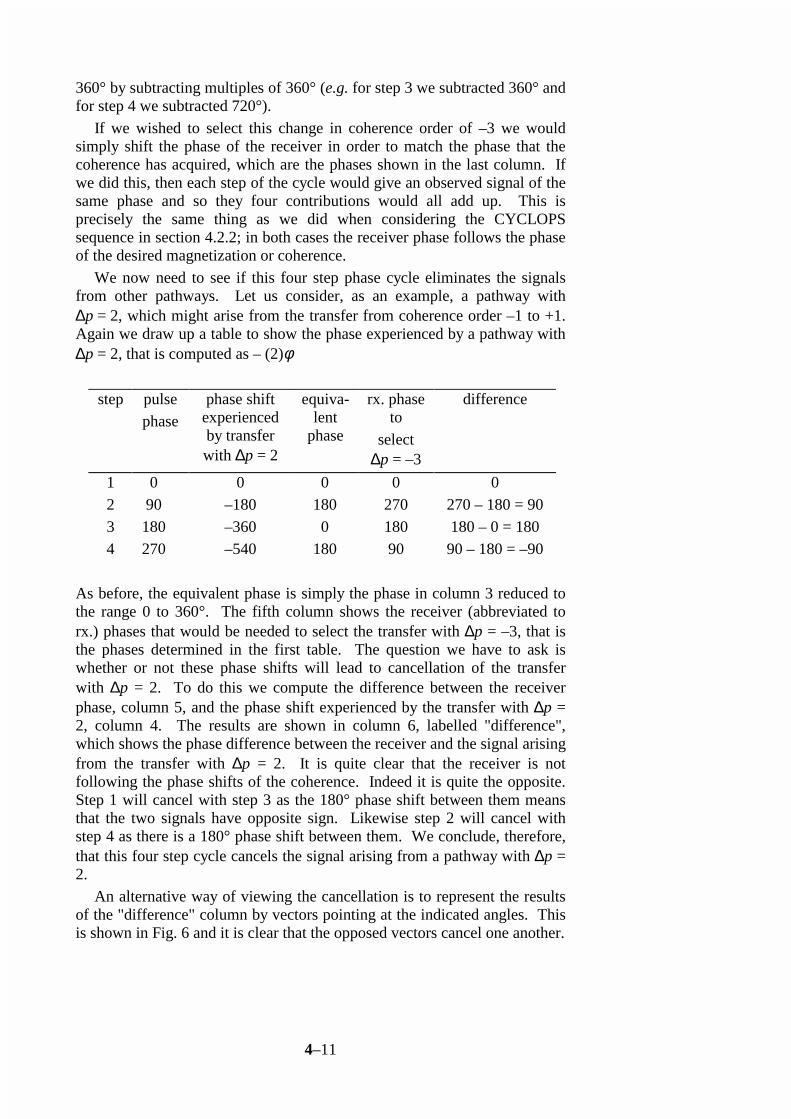
Figure 5 The pulse sequence for INEPT. In this diagram the filled rectangles represent 90° pulses and the open rectangles represent 180° pulses. Unless otherwise stated the pulses

have phase x.

With the phases and delays shown equilibrium magnetization of spin I, Iz, is transferred to spin S, appearing as the operator Sx. Equilibrium magnetization of S, Sz, appears as –Sy. Often this latter signal is an inconvenience and it is desirable to suppress it. The procedure is very simple. If we change the phase of the first I pulse from x to –x the final magnetization arising from transfer of the I magnetization to S becomes –Sx i.e. it changes sign. In contrast, the signal arising from equilibrium S magnetization is unaffected simply because the Sz operator is unaffected by the first 90° pulse to spin I. By repeating the experiment twice, once with the phase of the first pulse set to x and once with it set to –x, and then subtracting the two resulting signals, the undesired signal is cancelled and the desired signal adds. This simple difference experiment can be regarded as a two-step phase

4–7

cycle in which the first I pulse has phases 0 2 and the receiver follows with phases 0 2. The difference is achieved in the course of time averaging (i.e. as the time domain signals are accumulated from different scans) rather than by recording the signals separately and then subtracting them. It is easy to confirm that an alternative is to cycle the second I spin 90° pulse 0 2 along with a receiver phase of 0 2. However, cycling the S spin 90° pulse is not effective at separating the two sources of signal as they are affected in the same way by changing the phase of this pulse (see exercises). Difference spectroscopy reveals one of the key features of phase cycling: that is the need to identify a pulse whose phase affects differently the fate of the desired and undesired signals. Cycling the phase of this pulse can then be the basis of discrimination. In many experiments a simple cycle of 0 2 on a suitable pulse and the receiver is all that is required to select the desired signal. This is particularly the case in heteronuclear experiments, of which the INEPT sequence is the prototype. Indeed, even the phase cycling used in the most complex three- and four-dimensional experiments applied to labelled proteins is little more than this simple cycle repeated a number of times for different transfer steps.

4.2.4 Basic Concepts

Although we can make some progress in writing simple phase cycles by considering the vector picture, a more general framework is needed in order to cope with experiments which involve multiple quantum coherence and related phenomena. We also need a theory which enables us to predict the degree to which a phase cycle can discriminate against different classes of unwanted signals. A convenient and powerful way of doing both these things is to use the coherence transfer pathway approach.

4.2.4.1 Coherence Order

Coherences, of which transverse magnetization is one example, can be classified according to a coherence order, p, which is an integer taking values 0, ± 1, ± 2 ... Single quantum coherence has p = ± 1, double has p = ± 2 and so on; z-magnetization, "zz" terms and zero-quantum coherence have p = 0. This classification comes about by considering the way in which different coherences respond to a rotation about the z-axis. A coherence of

order p, represented by the density operator ( )σ p , evolves under a z-rotation of angle φ according to

( ) ( ) ( ) ( ) ( )exp exp exp− = −i i iφ σ φ φ σF F pzp

zp

[1]

where Fz is the operator for the total z-component of the spin angular momentum. In words, a coherence of order p experiences a phase shift of - pφ. Equation [1] is the definition of coherence order. As an example consider the pure double quantum operator for two coupled spins, 2I1xI2y + 2I1yI2x. This can be rewritten in terms of the raising and lowering operators for spin i, Ii

+ and I i− , defined as

4–8

I I I I I Ii ix iy i ix iy

+ = + = −i i–

to give ( )11 2 1 2i I I I I+ + − −− . The effect of a z-rotation on the raising and

lowering operators is, in the arrow notation,

( )I Ii

I

iiz± ± →φ φexp i .

Using this, the effect of a z-rotation on the term I I1 2+ + can be determined as

( ) ( ) ( )I I I I I II Iz z

1 2 1 2 1 21 2+ + + + + + → − → − −φ φφ φ φexp exp expi i i

Thus, as the coherence experiences a phase shift of –2φ the coherence is classified according to Eqn. [1] as having p = 2. It is easy to confirm that the term I I1 2

− − has p = −2. Thus the pure double quantum term, 2 21 2 1 2I I I Ix y y x+ , is an equal mixture of coherence orders +2 and –2.

As this example shows, it is possible to determine the order or orders of any state by writing it in terms of raising and lowering operators and then simply inspecting the number of raising and lowering operators in each term. A raising operator contributes +1 to the coherence order whereas a lowering operator contributes –1. A z-operator, Iiz, does not contribute to the overall order as it is invariant to z-rotations. Coherences involving heteronuclei can be assigned both an overall order and an order with respect to each nuclear species. For example the term I S1 1

+ − has an overall order of 0, is order +1 for the I spins and –1 for the S

spins. The term I I S z1 2 1+ + is overall of order 2, is order 2 for the I spins and

is order 0 for the S spins.

4.2.4.2 Phase Shifted Pulses

A radiofrequency pulse causes coherences to be transferred from one order to one or more different orders; it is this spreading out of the coherence which is responsible both for the richness of multiple-pulse NMR and for the need for phase cycling to select one transfer among many possibilities. An example of this spreading between coherence orders is the effect of a non-selective pulse on antiphase magnetization, such as 2I1xI2z, which corresponds to coherence orders ±1. Some of the coherence may be transferred into double- and zero-quantum coherence, some may be transferred into two-spin order and some will remain unaffected. The precise outcome depends on the phase and flip angle of the pulse, but in general we can see that there are many possibilities. If we consider just one coherence, of order p, and consider its transfer to a coherence of order p' by a radiofrequency pulse we can derive a very general result for the way in which the phase of the pulse affects the phase of the coherence. It is on this relationship that the phase cycling method is based.

4–9

We will write the initial state of order p as ( )σ p and represent the effect of the radiofrequency pulse causing the transfer by the unitary transformation U(φ)where φ is the phase of the pulse. The initial and final states are related by the usual transformation

( ) ( ) ( ) ( )U Up p0 0σ σ–1 = ′ + terms of other orders [2]

the other terms will be dropped as we are only interested in the transfer from p to p'. The transformation brought about by a radiofrequency pulse phase shifted by φ, U(φ), is related to that with the phase set to zero, U(0), by the rotation

( ) ( ) ( ) ( )U F U Fz zφ φ φ= −exp expi i0 [3]

Using this the effect of the phase shifted pulse on the initial state ( )σ p can

be written

( ) ( ) ( )( ) ( ) ( ) ( ) ( ) ( ) ( )

U U

F U F F U F

p

z zp

z z

φ σ φ

φ φ σ φ φ

–1

–exp exp exp exp

=

− −i i i i0 01

[4]

The central rotation of ( )σ p , ( ) ( ) ( )exp expi iφ σ φF Fzp

z− , can be replaced,

using Eqn. [1], by ( ) ( )exp i p pφ σ so that the right-hand side of Eqn. [4]

simplifies to

( ) ( ) ( ) ( ) ( ) ( )exp exp exp–1

i i ip F U U Fzp

zφ φ σ φ− 0 0

We now use Eqn. [2] to rewrite ( ) ( ) ( )U Up0 0σ –1 as ( )σ ′p thus giving

( ) ( ) ( ) ( )exp exp expi i ip F Fzp

zφ φ σ φ− ′

Once again we apply Eqn. [2] to determine the effect of the z-rotations on

the state ( )σ ′p, giving the final result

( ) ( ) ( ) ( ) ( )exp exp expi i ip p pp pφ φ σ φ σ− ′ = −′ ′∆ [5]

where the change is coherence order, ∆p, is defined as (p' − p). Returning to Eqn. [] we can now use Eqn. [5] to rewrite the right hand side and hence obtain the simple result

4–10

( ) ( ) ( ) ( ) ( )U U pp pφ σ φ φ σ–1exp= − ′i ∆ [6]

This relationship result tells us that if we consider a pulse which causes a change in coherence order of ∆p then altering the phase of that pulse by an angle φ will result in the coherence acquiring a phase label –∆p φ. In other words a particular change in coherence order acquires a phase label when the phase of the pulse causing that change is altered; the size of this label depends on the change in coherence order. It is this property which enables us to separate different changes in coherence order from one another by altering the phase of the pulse. Before seeing how this key relationship is used in practice there are two remarks to make. The first concerns the transformation U(φ). We have described this as being due to a radiofrequency pulse, but in fact any sequence of pulses and delays can be represented by such a transformation so our final result is general. Thus we can, for the purposes of analysing the effects of a pulse sequence, group one or more pulses and delays together and simply consider them as a single unit causing a transformation from one coherence order to another. The whole unit can be phase shifted by shifting the phase of all the pulses in the unit. We shall see some practical applications of this later on. The second comment to make concerns the phase which is acquired by the transferred coherence: this phase appears as a phase shift of the final observed signal, i.e. the position of the observed magnetization in the xy-plane at the start of acquisition. A particular coherence may undergo several transformations before it is observed finally , but at each stage these phase shifts are carried forward and so affect the final signal. Thus, although the coherence of order p' resulting from the transformation U may not itself be observable, any phase it acquires in the course of the transformation will ultimately be observed as a phase shift in the observed signal derived from this coherence.

4.2.4.3 Selection of a Single Pathway

To focus on the issue at hand let us consider the case of transferring from coherence order +2 to order –1. Such a transfer has ∆p = (–1 – (2) ) = –3. Let us imagine that the pulse causing this transformation is cycled around the four cardinal phases (x, y, –x, –y, i.e. 0°, 90°, 180°, 270°) and draw up a table of the phase shift that will be experienced by the transferred coherence. This is simply computed as – ∆p φ, in this case = – (–3)φ.

step pulse phase phase shift experienced by transfer with ∆p = –3

equivalent phase

1 0 0 0 2 90 270 270 3 180 540 180 4 270 810 90

The fourth column, labelled "equivalent phase", is just the phase shift experienced by the coherence, column three, reduced to be in the range 0 to

4–11

360° by subtracting multiples of 360° (e.g. for step 3 we subtracted 360° and for step 4 we subtracted 720°). If we wished to select this change in coherence order of –3 we would simply shift the phase of the receiver in order to match the phase that the coherence has acquired, which are the phases shown in the last column. If we did this, then each step of the cycle would give an observed signal of the same phase and so they four contributions would all add up. This is precisely the same thing as we did when considering the CYCLOPS sequence in section 4.2.2; in both cases the receiver phase follows the phase of the desired magnetization or coherence. We now need to see if this four step phase cycle eliminates the signals from other pathways. Let us consider, as an example, a pathway with ∆p = 2, which might arise from the transfer from coherence order –1 to +1. Again we draw up a table to show the phase experienced by a pathway with ∆p = 2, that is computed as – (2)φ

step pulse phase

phase shift experienced by transfer with ∆p = 2

equiva-lent

phase

rx. phase to

select ∆p = –3

difference

1 0 0 0 0 0 2 90 –180 180 270 270 – 180 = 90 3 180 –360 0 180 180 – 0 = 180 4 270 –540 180 90 90 – 180 = –90

As before, the equivalent phase is simply the phase in column 3 reduced to the range 0 to 360°. The fifth column shows the receiver (abbreviated to rx.) phases that would be needed to select the transfer with ∆p = –3, that is the phases determined in the first table. The question we have to ask is whether or not these phase shifts will lead to cancellation of the transfer with ∆p = 2. To do this we compute the difference between the receiver phase, column 5, and the phase shift experienced by the transfer with ∆p = 2, column 4. The results are shown in column 6, labelled "difference", which shows the phase difference between the receiver and the signal arising from the transfer with ∆p = 2. It is quite clear that the receiver is not following the phase shifts of the coherence. Indeed it is quite the opposite. Step 1 will cancel with step 3 as the 180° phase shift between them means that the two signals have opposite sign. Likewise step 2 will cancel with step 4 as there is a 180° phase shift between them. We conclude, therefore, that this four step cycle cancels the signal arising from a pathway with ∆p = 2. An alternative way of viewing the cancellation is to represent the results of the "difference" column by vectors pointing at the indicated angles. This is shown in Fig. 6 and it is clear that the opposed vectors cancel one another.

4–12

stepdifference 0° 90° 180° -90°

1 2 3 4

0°

Figure 6. A visualisation of the phases from the "difference" column.

Next we consider the coherence transfer with ∆p = +1. Again, we draw up the table and calculate the phase shifts experience by this transfer from – (+1)φ.

Step pulse phase

phase shift experienced by transfer

with ∆p = +1

equiva-lent

phase

rx. phase to

select ∆p = –3

difference

1 0 0 0 0 0 2 90 –90 270 270 270 – 270 = 0 3 180 –180 180 180 180 – 180 = 0 4 270 –270 90 90 90 – 90 = 0

Here we see quite different behaviour. The equivalent phases, that is the phase shifts experienced by the transfer with ∆p = 1, match exactly the receiver phase determined for ∆p = –3, thus the phases in the "difference" column are all zero. We conclude that the four step cycle selects transfers both with ∆p = –3 and +1. Some more work with tables such as these (see exercises) will reveal that this four step cycle suppresses contributions from changes in coherence order of –2, –1 and 0. It selects ∆p = –3 and 1. It also selects changes in coherence order of 5, 9, 13 and so on. This latter sequence is easy to understand. A pathway with ∆p = 1 experiences a phase shift of –90° when the pulse is shifted in phase by 90°; the equivalent phase is thus 270°. A pathway with ∆p = 5 would experience a phase shift of –5 × 90° = –450° which corresponds to an equivalent phase of 270°. Thus the phase shifts experienced for ∆p = 1 and 5 are identical and it is clear that a cycle which selects one will select the other. The same goes for the series ∆p = 9, 13 ...

The extension to negative values of ∆p is also easy to see. A pathway with ∆p = –3 experiences a phase shift of 270° when the pulse is shifted in phase by 90°. A transfer with ∆p = +1 experiences a phase of –90° which corresponds to an equivalent phase of 270°. Thus both pathways experience the same phase shifts and a cycle which selects one will select the other. The pattern is clear, this four step cycle will select a pathway with ∆p = −3, as it was designed to, and also it will select any pathway with ∆p = −3 + 4n where n = ±1, ±2, ±3 ...

4–13

4.2.4.4 General Rules

The discussion in the previous section can be generalised to the following: Consider a phase cycle in which the phase of a pulse takes N evenly spaced steps covering the range 0 to 2π radians i.e. the phases, φk, are 2πk/N where k = 0, 1, 2 ... (N – 1). To select a change in coherence order, ∆p, the receiver phase is set to –∆p × φk for each step and all the resulting signals are summed. This cycle will, in addition to selecting the specified change in coherence order, also select pathways with changes in coherence order ∆p ± nN where n = ±1, ±2 ..

The way in which phase cycling selects a series of values of ∆p which are related by a harmonic condition is closely related to the phenomenon of aliasing in Fourier transformation. Indeed, the whole process of phase cycling can be seen as the computation of a discrete Fourier transformation with respect to the pulse phase. The Fourier co-domains are phase and coherence order. The fact that a phase cycle inevitably selects more than one change in coherence order is not necessarily a problem. We may actually wish to select more than one pathway, and examples of this will be given below in relation to specific two-dimensional experiments. Even if we only require one value of ∆p we may be able to discount the values selected at the same time as being improbable or insignificant. In a system of m coupled spins one-half, the maximum order of coherence that can be generated is m, thus in a two spin system we need not worry about whether or not a phase cycle will discriminate between double quantum and six quantum coherences as the latter simply cannot be present. Even in more extended spin systems the likelihood of generating high-order coherences is rather small and so we may be able to discount them for all practical purposes. If a high level of discrimination between orders is needed, then the solution is simply to use a phase cycle which has more steps i.e. in which the phases move in smaller increments. For example a six step cycle will discriminate between ∆p = +2 and +6, whereas a four step cycle will find these to be identical.

4.2.4.5 Coherence Transfer Pathways

In multiple-pulse NMR it is important to specify the coherences which should be present at each stage of the sequence. This is conveniently done using a coherence transfer pathway (CTP) diagram. Figure 7 shows such a diagram for the DQF COSY sequence.

t1 t2

210

-1-2

4–14

Figure 7. The pulse sequence and coherence transfer pathway for DQF COSY.

The solid lines under the sequence represent the coherence orders required during each part of the sequence; as expected the pulses cause changes in coherence order. In this example we have more that one coherence order present in some of the time periods; this is a common feature. In addition we notice that the second pulse causes a transfer between orders ±1 and ±2, with all connections being present. Again, such a "fanning out" of the coherence transfer pathway is common in many experiments. There are a number of remarks to be made about the CTP diagram. Firstly, we should remember that this pathway is just the desired pathway and that it must be established separately that the pulse sequence and the spin system itself is capable of supporting the specified coherences. Thus the DQF COSY sequence could be applied, along with a suitable phase cycle to select the specified pathway, to uncoupled spins but we would not expect to see any peaks in the spectrum. Likewise, the sequence itself must be designed appropriately, the phase cycle cannot select something that the pulse sequence does not generate. The second point to note is that the coherence transfer pathway must start with p = 0, that is the coherence order which corresponds to equilibrium magnetization. In addition, the pathway has to end with |p| = 1 as it is only single quantum coherence that is observable. If one uses quadrature detection, that is the method described in section 4.2.1 in which effectively both the x and y components of the magnetization are measured, it turns out that one is observing either p = +1 or –1. The usual convention, which fits in with the normal convention for the sense of rotation, is to assume that we are detecting p = –1; we shall use this throughout. Finally, we note that only a limited number of possible coherence orders are shown - in this case just those between –2 and +2. As was discussed above we need to remember that the spin system may be capable of supporting higher orders of coherence and take this into account when designing the phase cycle.

4.2.4.6 Refocusing Pulses

180° pulses give rise to a rather special coherence transfer pathway: they simply change the sign of the coherence order. We can see how this arises by considering the effect of a 180° pulse to the operators Ii

+ and Ii−

I IiI

iix± →π #

The operator on the right simply has the opposite sign of coherence order to that on the left. The same will be true of all of the raising or lowering operators of the different spins present and affected by the 180° pulse; the result is also valid, to within a phase factor, for any phase of the pulse (see exercises). We can now derive the EXORCYLE phase cycle using this property. Consider a spin echo and the coherence transfer diagram shown in Fig. 8.

4–15

Figure 8. A spin echo and the corresponding CTP.

As discussed above, the CTP starts with coherence order 0 and ends with order –1. Since the 180° pulse simply swaps the sign of the coherence order, the order +1 must be present prior to the 180° pulse. Thus the 180° pulse is causing the transformation from +1 to –1, which is a ∆p of –2. A phase cycle of four steps is easy to draw up

step phase of 180° pulse

phase shift experienced by transfer with ∆p = –2

equivalent phase = rx. phase

1 0 0 0 2 90 180 180 3 180 360 0 4 270 540 180

The phase cycle is thus 0 1 2 3 for the 180° pulse and 0 2 0 2 for the receiver, which is just EXORCYCLE. As the cycle has four steps, the pathway with ∆p = +2 is also selected (shown dotted in Fig. 8). Although this pathway does not lead to an observable signal in this experiment its simultaneous selection in multiple pulse experiments where further pulses follow the spin echo is a useful feature. An eight step cycle can be used to select the refocusing of double quantum in which the transfer is from p = +2 to –2 (i.e. ∆p = –4) or vice versa (see exercises). A two step cycle, 0 2 for the 180° pulse and 0 0 for the receiver, will select all even values of ∆p (see exercises).

4.2.5 Lineshapes and Frequency Discrimination

The selection of a particular coherence transfer pathway is closely connected to two important aspects of multi-dimensional NMR experiments, that of frequency discrimination and lineshape selection. By frequency discrimination we mean the steps taken to ensure that the signs of the frequencies of the coherences evolving the indirectly detected domains can be determined. Typically this is done by using the States-Haberkorn-Ruben or TPPI methods. Lineshape selection is closely associated with frequency discrimination, and a particular frequency discrimination method results in a particular lineshape in the indirectly detected domains. It is clearly a priority to obtain the best lineshape possible, which generally means an absorption mode line. The issues are the same for two- and higher-dimensional spectra so we will consider just the simplest case. A typical two-dimensional experiment "works" by transferring a component of magnetization, say of spin i, present at the end of the evolution time, t1, through some mixing process to another spin, say j. The size of the transferred component varies as a function of t1; it is said to be

4–16

modulated in t1. If the modulation frequency is Ωi then the final steps of the two-dimensional experiment can be represented as

cos cosΩ Ωi ix i jxt I t I1 1

mixing → [7]

where we have assumed that the x-component is transferred. The signal is detected during t2 in the usual way, using the detection scheme (called quadrature detection) described in section 4.2.1. This results in a signal which can be considered as a complex quantity and can be written as

( )cos expΩ Ωi jt t1 2i

Such a signal is said to be amplitude modulated in t1. If we return to the mixing step sketched in Eqn. [7] we can reveal the underlying processes by re-writing the operators Iix in terms of the raising and lowering operators

[ ]12 1

12 1cos cosΩ Ωi i i i jxt I I t I+ −+ →mixing

[8]

The implication of this is that to obtain amplitude modulation coherence orders +1 and –1 must both contribute, and contribute equally, to the transferred signal. This is the condition for obtaining amplitude modulation, and phase cycles for two- and higher-dimensional experiments need to be written in such a way as to retain "symmetrical pathways" in t1. Once this has been achieved, frequency discrimination can be added by using one of the usual methods. It is possible to use a phase cycle to achieve frequency discrimination. One simply writes a cycle which selects one coherence order, i.e. p = +1, during t1. In effect what this achieves is the selection of transfer (mixing) from one operator, such as Ii

+ , rather than from the combination of Ii+ and

Ii− given in Eqn. [8]. Since under free evolution the operator Ii

+ simply

acquires a phase term, of the form of exp(i Ωi t1), the resulting signal is phase modulated in t1 and thus frequency discrimination is achieved. Such a procedure is called echo-/anti-echo selection, or P-/N-type selection. It is illustrated in the following section for the simple COSY experiment.

4.2.5.1 P- and N-Type COSY

t1 t2

10

-1

Figure 9. The pulse sequence for COSY with the CTP for the P-type spectrum shown as the solid line, and that for the N-type spectrum as a dashed line.

4–17

Figure 9 shows the simple COSY pulse sequence and two possible (and alternative) coherence transfer pathways. Both pathways start with p = 0 and end with p = –1, as described above. They differ, however, in the sign of the coherence order present during t1. In the first case (the solid line) the order present is p = –1, the same as present during acquisition. Such a spectrum will be frequency discriminated, as was described above, and a diagonal peak at a positive offset in F2 will also be at a positive offset in F1. In contrast, a spectrum recorded such that p = +1 is present during t1 (the dotted line) will have opposite offsets in the two dimensions. This arises because although the operators Ii

+ and Ii− both acquire a phase dependent

on the offset Ωi, the sign of this phase modulation is opposite. In the usual notation

( )I t Ii

t I

i i

i iz± ± →Ω

Ω1

1exp i

Selection of one of these pathways gives a signal which is phase modulated in both t1 and t2. Subsequent two-dimensional Fourier transformation will give a peak in the spectrum which has the phase-twist lineshape. This is not a suitable lineshape high-resolution work and thus this method of selection is not generally used in demanding applications. The spectrum in which the sign of the modulating frequencies, and hence the sign of the coherence order, is the same in t1 and t2 is called the P-type or anti-echo spectrum. Where these signs are opposite, one obtains the N-type or echo spectrum. The echo/anti-echo terminology arises because the pathway leading to the echo spectrum has ∆p = –2 for the last pulse, which is analogous to the spin echo and indeed this pulse does result in partial refocusing of inhomogeneous broadening. The phase cycles are simple to construct. We first note a short-cut in that the first pulse can only generate transverse magnetization from z-magnetization. It is quite impossible for it to generate multiple quantum coherence. Thus we can assume that the only p = ±1 are present during t1. Our attention is therefore focused on the last pulse. In the case of the N-type spectrum we need to select the pathway with ∆p = –2, and we have already devised a cycle to do this in section 4.2.4.6 - it is simply EXORCYCLE in which the last 90° pulse goes 0 1 2 3 and the receiver goes 0 2 0 2. To select the P-type spectrum the required pathway has ∆p = 0, for which the phase cycle is simply 0 1 2 3 on the final 90° pulse and 0 0 0 0 on the receiver, i.e. as ∆p = 0 the coherence pathway experiences no phase shifts. Of course the unwanted pathways will experience phase shifts and thus will be cancelled. If multiple quantum coherence is present during t1 of a two-dimensional experiment the same principles apply, although smaller steps will be needed in order to select the required pathways (see exercises).

4–18

4.2.6 The Tricks of the Trade

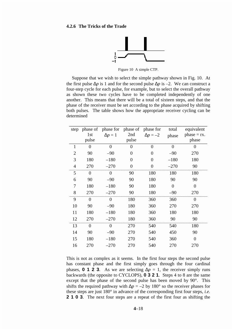
Figure 10 A simple CTP.

Suppose that we wish to select the simple pathway shown in Fig. 10. At the first pulse ∆p is 1 and for the second pulse ∆p is –2. We can construct a four-step cycle for each pulse, for example, but to select the overall pathway as shown these two cycles have to be completed independently of one another. This means that there will be a total of sixteen steps, and that the phase of the receiver must be set according to the phase acquired by shifting both pulses. The table shows how the appropriate receiver cycling can be determined

step phase of 1st

pulse

phase for ∆p = 1

phase of 2nd

pulse

phase for ∆p = –2

total phase

equivalent phase = rx.

phase

1 0 0 0 0 0 0 2 90 –90 0 0 –90 270 3 180 –180 0 0 –180 180 4 270 –270 0 0 –270 90

5 0 0 90 180 180 180 6 90 –90 90 180 90 90 7 180 –180 90 180 0 0 8 270 –270 90 180 –90 270

9 0 0 180 360 360 0 10 90 –90 180 360 270 270 11 180 –180 180 360 180 180 12 270 –270 180 360 90 90

13 0 0 270 540 540 180 14 90 –90 270 540 450 90 15 180 –180 270 540 360 0 16 270 –270 270 540 270 270

This is not as complex as it seems. In the first four steps the second pulse has constant phase and the first simply goes through the four cardinal phases, 0 1 2 3. As we are selecting ∆p = 1, the receiver simply runs backwards (the opposite to CYCLOPS), 0 3 2 1. Steps 4 to 8 are the same except that the phase of the second pulse has been moved by 90°. This shifts the required pathway with ∆p = –2 by 180° so the receiver phases for these steps are just 180° in advance of the corresponding first four steps, i.e. 2 1 0 3. The next four steps are a repeat of the first four as shifting the

4–19

phase of the second pulse by 180° results in a complete rotation of the coherence and so there is no net effect. The final four steps are the same as the second four, except that the second pulse is shifted by 270°. The key to devising these sequences is to simply work out the two four-step cycles independently and the merge them together rather than trying to work on the whole cycle. One writes down the first four steps, and then duplicates this four times as the second pulse is shifted. You should get the same steps, in a different sequence, if you shift the phase of the second pulse in the first four steps (see exercises). We can see that the total size of a phase cycle grows at an alarming rate. With only four phases for each pulse the number of steps grows as 4l where l is the number of pulses in the sequence. A prospect of a 64 step phase cycle for simple experiments like NOESY and DQF COSY is a daunting one. We may not wish to repeat each t1 increment 64 times, although of course if the spectrum were weak we may end up doing this anyway simply to improve the signal-to-noise ratio. The "trick" to learn is that you need not phase cycle each pulse. For various reasons there are shortcuts which can be used to reduce the number of pulses which need to be cycled. To find out what these shortcuts are you need to understand how the pulse sequence works and what all the pulses do. Sometimes, we can make shortcuts by ignoring certain possibilities, on the grounds that there are unlikely and that if they do occur they will sufficiently rare to be tolerable. We will illustrate all of these points with reference to the DQF COSY pulse sequence, shown in Fig. 7 along with its coherence transfer diagram. We have already noted the need to retain the p = ±1 pathways during t1 in order to be able to compute an absorption mode spectrum. Note also that the coherence orders ±1 in t1 are each connected to p = ±2 during the double quantum filter delay and that both of these double quantum levels are connected to p = –1 which is observed. A detailed analysis of this sequence will show that in general all of these pathways are present and equally likely.

4.2.6.1 The First Pulse

We have already commented on this in relation to the COSY experiment. Starting from equilibrium magnetization, Iiz, a simple pulse can generate only transverse magnetization with coherence orders ±1. Thus it is not necessary to cycle this first pulse to select the pathway shown in Fig. 7. We note here for completeness that the first pulse, if it is imperfect, may leave some magnetization along the z-axis and thus the fate of this magnetization needs to be considered in relation to the rest of the pulse sequence. This residual z-magnetization is present during t1 as coherence order zero. We will return to this in section 4.2.6.4.

4.2.6.2 Grouping Pulses Together

In section 4.2.4.2 we noted that the phase shift of a particular pathway by – ∆p φ applied for the case where the transfer was brought about by a single pulse or by a group of pulses (and delays) whose phases are moved together. Essentially we are regarding the group of pulses as a single entity and may

4–20

phase cycle it in such a way as to select a particular value of ∆p. It is important to realise, however, that the selection will simply be for a particular change in coherence order brought about by the whole group of pulses. The phase cycle will not select for what coherence transfers take place in the group. The idea of grouping pulses together thus has to be used carefully as it may lead to ambiguities. In the DQF COSY sequence we have already noted that the pathways ∆p = ±1 are inherently selected by the first pulse, so we should create no ambiguity by simply grouping the first two pulses together and cycling them as a unit to select the overall pathway ∆p = ±2. Such a move will retain the symmetrical pathways required during t1 and the complex series of transfers brought about by the second pulse are selected inherently. If we use a four-step cycle to select ∆p = +2, we will also select –2 at the same time, which is just what we require. The cycle is devised in the usual way

step phase of first two pulses

phase for ∆p = +2

phase for ∆p = –2

equivalent phase = rx. phase

1 0 0 0 0 2 90 –180 180 180 3 180 –360 360 0 4 270 –540 540 180

The equivalent phase is the same for both pathways, ∆p = ±2. The overall phase cycle is thus for the first two pulses to go 0 1 2 3, the third pulse to remain fixed and the receiver to go 0 2 0 2. We shall see in the next section that this is sufficient to select the required pathway.

The four-step cycle also selects ∆p = ±6, so there is the possibility of signals arising due to filtration through six-quantum coherence. In normal spin systems the amount of such high order coherences that can be generated is usually very small so that in practice we can discount this possibility. Finally, we need to consider z-magnetization which may be left over after an imperfect initial 90° pulse or which arises due to relaxation during t1. If signals are derived from such magnetization they give rise to peaks at F1 = 0 in the spectrum simply because magnetization does not precess during t1 and so has no frequency label; such peaks are called axial peaks. z-Magnetization present at the end of t1 will be turned to the transverse plane by the second 90° pulse, generating coherences ±1 as before. The second pulse is being cycled 0 1 2 3 along with the receiver going 0 2 0 2; such a cycle suppresses the pathway ∆p = ±1 and so axial peaks are suppressed.

4.2.6.3 The Last Pulse

The final pulse in a sequence has some special features which may be exploited when trying to reduce a phase cycle to its minimum. This pulse may cause transfer to many different orders of coherence but only one of these, that with p = –1, is observable. Thus, if we have already selected, in

4–21

an unambiguous way, a particular set of coherence orders present just before the last pulse, no further cycling of this pulse is needed. The fact that we can only observe p = –1 will "naturally" select what we want. The DQF COSY phase cycle proposed in the previous section achieves this result in that it selects p = ±2 just before the last pulse. No further cycling is required, therefore. We can view this property of the final pulse in a different way. Looking at the DQF COSY sequence we see that the two required pathways to be brought about by the final pulse have ∆p= –3 and +1. As the only detectable signal has p = –1, the selection of these two pathways will guarantee that the only contributors to the observed signal will be from coherences with orders p = ±2 present just before this pulse. Cycling just the last pulse will thus achieve all that we require. In section 4.2.6 we have already devised a phase cycle to select ∆p = +1, the pulse goes 0 1 2 3 and the receiver goes 0 3 2 1. As this is a four-step cycle we see immediately that ∆p = –3 is also selected, which is what is required. Other, higher order pathways are selected, such as ∆p = +5 or –7; these can most probably be ignored safely. Finally we ought to consider the fate of any z-magnetization present at the end of t1. This is turned to coherence orders ±1 by the second pulse and so for it to be observable (i.e. p = –1) during acquisition it must undergo a transfer by the last pulse of ∆p = 0 or –2. Both of these are blocked by the phase cycle, so axial peaks are suppressed. We now have two alternative four step cycles for DQF COSY; in section 4.2.6.5, we will show that despite their different origins they are more or less the same.

4.2.6.4 Axial Peak Suppression

Sometimes we want to write a phase cycle in which there is an added explicit step to suppress axial peaks. In principle and strictly according to theory this is not always necessary as the magnetization that leads to axial peaks is often suppressed by the phase cycle used for coherence selection. A simple two step phase cycle suffices for this suppression. The first pulse is supposed to result in the pathway ∆p = ±1 and such a pathway is selected, along with others, using the two step cycle in which the pulse goes 0 2 and the receiver goes 0 2 also. Any magnetization which arrives at the receiver but which has not experienced the phase shift from the first pulse will be cancelled. The cycle thus eliminates all peaks in the spectrum, such as axial peaks, which do not arise from the first pulse. Of course this two-step cycle does not select exclusively ∆p = ±1, but most importantly it does reject ∆p = 0 which is one likely source of axial peaks.

4.2.6.5 Shifting the Whole Sequence

If we group all of the pulses in the sequence together and regard them as a unit they simply achieve the transformation from equilibrium magnetization, p = 0, to observable magnetization, p = –1. They could be cycled as a group to select this pathway with ∆p = –1, that is the pulses going 0 1 2 3 and the receiver going 0 1 2 3. This is of course the

4–22

CYCLOPS phase cycle. If time permits we sometimes add CYCLOPS-style cycling of all of the pulses in the sequence so as to suppress some artefacts associated with imperfections in the receiver. Adding such cycling does, of course, extend the phase cycle by a factor of four. This idea of shifting all of the pulses in the sequence has other applications. Consider the DQF COSY phase cycle proposed in section 4.2.6.3:

step 1st pulse 2nd pulse 3rd pulse receiver

1 0 0 0 0 2 0 0 90 270 3 0 0 180 180 4 0 0 270 90

Suppose we decide, for some reason, that we do not want to shift the receiver phase, but want to keep it fixed at phase zero. If we add 90° to the phase of all the pulses in step 2, then we will need also to add 90° to the receiver as the overall transformation is ∆p = –1; this puts the receiver phase at 0°. In the same way we can add 180° to all the pulses and the receiver for step 3 and 270° for step 4. Once all the phases are reduced to the usual range of 0 to 360° we have

step 1st pulse 2nd pulse 3rd pulse receiver

1 0 0 0 0 2 90 90 180 0 3 180 180 0 0 4 270 270 180 0

The result looks rather strange, as we seem to be shifting the phase of all of the pulses at the same time. However, we know that, in a formal way, it is exactly the same cycle as was devised in section 4.2.6.3 By writing it in this way, however, the way in which the cycle works is rather obscured. In the case of DQF COSY there is probably no reason for adopting this procedure. However, a case where it might be useful is when a phase cycle calls for phase shifts of other than multiples of 90° for the receiver. Some spectrometers allow fine resolution phase shifting of the pulse phase, but only allow 90° steps for the receiver. In such cases the required phase shifts of the received can be generated in effect by moving the phase of all the pulses until the receiver phases are at multiples of 90° (see exercises). We can play one last trick with the phase cycle given in the table. As the third pulse is required to achieve the transformation ∆p = –3 or +1 we can alter its phase by 180° and compensate for this by shifting the receiver by 180° also. We apply this trick to the phase of the third pulse for steps 2 and 4 to give the cycle

4–23

step 1st pulse 2nd pulse 3rd pulse receiver

1 0 0 0 0 2 90 90 0 180 3 180 180 0 0 4 270 270 0 180

This is just the cycle proposed in section 4.2.6.2. We have then three different phase cycles, each of which, despite looking rather different achieves the same result.

4.2.7 More Examples

4.2.7.1 Homonuclear Experiments

t1 t2

210

-1-2

Figure 11 The pulse sequence and CTP for double-quantum spectroscopy.

Double Quantum Spectroscopy: A simple sequence for double quantum spectroscopy is shown in Fig. 11; note the retention of both pathways with p = ±1 during the initial spin echo and with p = ±2 during t1. There are a number of possible phase cycles for this experiment and, not surprisingly, they are essentially the same as those for DQF COSY. If we regard the first three pulses as a unit, then they are required to achieve the overall transformation ∆p = ±2, which is the same as that for the first two pulses in the DQF COSY sequence. Thus the same cycle can be used with these three pulses going 0 1 2 3 and the receiver going 0 2 0 2. Alternatively the final pulse can be cycled 0 1 2 3 with the receiver going 0 3 2 1, as in section 4.2.6.3. Both of these phase cycles can be extended by EXORCYCLE phase cycling of the 180° pulse, resulting in a total of 16 steps (see exercises).

t1 t2

10

-1

m ix

Figure 12. The pulse sequence and CTP for NOESY.

NOESY: The sequence is shown in Fig. 12. Again it can be viewed in two ways. If we group the first two pulses together they are required to achieve

4–24

the transformation ∆p = 0 and this leads to a four step cycle in which the pulses go 0 1 2 3 and the receiver remains fixed as 0 0 0 0. In this experiment axial peaks arise due to z-magnetization recovering during the mixing time, and this cycle will not suppress these contributions as there is no suppression of the pathway ∆p = –1 caused by the last pulse. Thus we need to add axial peak suppression, which is conveniently done by adding the simple cycle 0 2 on the first pulse and the receiver. The final 8 step cycle is 1st pulse: 0 1 2 3 2 3 0 1, 2nd pulse: 0 1 2 3 0 1 2 3, 3rd pulse fixed, receiver: 0 0 0 0 2 2 2 2.

An alternative is to cycle the last pulse to select the pathway ∆p = –1, giving the cycle 0 1 2 3 for the pulse and 0 1 2 3 for the receiver. Once again, this does not discriminate against z-magnetization which recovers during the mixing time, so a two step phase cycle to select axial peaks needs to be added (see exercises).

4.2.7.2 Heteronuclear Experiments

The phase cycling for most heteronuclear experiments tends to be rather trivial in that the usual requirement is simply to select that component which has been transferred from one nucleus to another. We have already seen in section 4.2.3 that this simply boils down to a 0 2 phase cycle on a pulse accompanied by the same on the receiver i.e. a difference experiment. The choice of which pulse to cycle depends more on practical problems associated with difference spectroscopy than with any fundamental theoretical considerations. HMQC: The pulse sequence for HMQC is given in Fig. 13, along with a coherence transfer pathway. We have written a separate pathway for the two nuclear species, thus the heteronuclear multiple quantum coherence which gives the sequence its name appears as a combination of pI = ±1 and pS = ±1. Again, all symmetrical pathways are retained in order to give optimum sensitivity and pure phase lineshapes.

t1

t2

10

-1

10

-1

∆∆I

S

p I

p S

Figure 13. The pulse sequence and CTP for HMQC. Separate pathways are shown for the I and S spins.

The essential result we need to achieve in this sequence is to suppress the signals arising from I spins which are not coupled to S spins. This is

4–25

achieved by cycling the phase of a pulse which affects the phase of the required coherence and which does not affect that of the unwanted coherence. The obvious targets are the two S spin 90° pulses, each of which is required to give the transformation ∆pS = ±1. A two step cycle with either of these pulses going 0 2 and the receiver doing the same will select this pathway and, by difference, suppress any I spin magnetization which has not been passed into multiple quantum coherence. It is also common to add EXORCYCLE phase cycling to the I spin 180° pulse, giving a cycle with eight steps overall. Axial peaks should be suppressed by the two step cycle of one of the S spin 90° pulses. It is clear that for heteronuclear experiments the coherence transfer pathway approach is not really necessary.

4.2.8 Conclusions

We have seen that phase cycling is a relatively straightforward method of selecting a particular coherence transfer pathway. Even at a theoretical level the method sometimes fails when we are trying to select a complex pathway, particularly one in which we are trying to select may parallel pathways (see exercises); it may not be possible to write a phase cycle which selects the required pathway. In practice phase cycling suffers from two major problems. The first is that the need to complete the cycle imposes a minimum time on the experiment. In two- and higher-dimensional experiments this minimum time can become excessively long, far longer than would be needed to achieve the desired signal-to-noise ratio. In such cases the only way of reducing the experiment time is to record fewer increments of the indirect times which has the undesirable consequence of reducing the limiting resolution in these dimensions. The second problem is that phase cycling always relies on recording all possible contributions and then cancelling out the unwanted ones by combining subsequent signals. If the spectrum has high dynamic range, or if spectrometer stability is a problem, this cancellation is less than perfect. The result is unwanted signals appearing in the spectrum and t1-noise in two-dimensional spectra. These problems become acute when dealing with proton detected heteronuclear experiments on natural abundance samples, or in trying to record spectra with intense solvent resonances. Both of these problems are alleviated to a large extent by moving to an alternative method of selection, the use of field gradient pulses which are the subject of the next section. However, this alternative method is not without its own difficulties and it is by no means a universal panacea. Neither phase cycling nor field gradient pulses can discriminate between z-magnetization and homonuclear zero-quantum coherence, both of which have coherence order zero. There are methods which can be used to suppress the contribution from zero-quantum coherence; these are all based on the fact that this coherence acquires a phase during a delay or period of spin-locking. There thus exists the possibility of cancellation or dephasing. Further details can be found in section 4.3.7.1.

4–26

4.3.1 Introduction

Field gradient pulses can be used to select particular coherence transfer pathways and, as we shall see, selection using gradients offers some advantages when compared to selection using phase cycling. During a pulsed field gradient the applied magnetic field is made deliberately spatially inhomogeneous for a short time. As a result, transverse magnetization and other coherences dephase across the sample and are apparently lost. However, this loss can be reversed by the application of a subsequent gradient which undoes the dephasing process thus restoring the magnetization or coherence. The crucial property of the dephasing process is that it proceeds at a different rate for different coherences. For example, double-quantum coherence dephases twice as fast as single-quantum coherence. Thus, by applying gradient pulses of different strengths or durations it is possible to refocus coherences which have, for example, been changed from single- to double-quantum by a radiofrequency pulse. Gradient pulses are introduced into the pulse sequence in such a way that only the wanted signals are observed in each experiment. Thus, in contrast to phase cycling, there is no reliance on subtraction of unwanted signals, and it can thus be expected that the level of t1-noise will be much reduced. Again in contrast to phase cycling, no repetitions of the experiment are needed, enabling the overall duration of the experiment to be set strictly in accord with the required resolution and signal-to-noise ratio. The properties of gradient pulses and the way in which they can be used to select coherence transfer pathways have been known since the earliest days of multiple-pulse NMR. However, their wide application in the past has been limited by technical problems which made it difficult to use such pulses in high-resolution NMR. The problem is that switching on the gradient pulse induces currents in any nearby conductors, such as the probe can and magnet bore tube. These induced currents, called eddy currents, themselves generate magnetic fields which perturb the NMR spectrum. Typically, the eddy currents are large enough to disrupt severely the spectrum and can last many hundreds of milliseconds. It is thus impossible to observe a high-resolution spectrum immediately after the application of a gradient pulse. Similar problems have beset NMR imaging experiments and have led to the development of shielded gradient coils which do not produce significant magnetic fields outside the sample volume and thus minimise the generation of eddy currents. The use of this technology in high-resolution NMR probes has made it possible to observe spectra within tens of microseconds of applying a gradient pulse. With such apparatus, the use of field gradient pulses in high resolution NMR is quite straightforward, a fact first realised and demonstrated by Hurd whose work has pioneered this whole area.

4–27

4.3.2 Selection with Gradient Pulses

4.3.2.1 Dephasing Caused by Gradients

A field gradient pulse is a period during which the B0 field is made spatially inhomogeneous; for example an extra coil can be introduced into the sample probe and a current passed through the coil in order to produce a field which varies linearly in the z-direction. We can imagine the sample being divided into thin discs which, as a consequence of the gradient, all experience different magnetic fields and thus have different Larmor frequencies. At the beginning of the gradient pulse the vectors representing transverse magnetization in all these discs are aligned, but after some time each vector has precessed through a different angle because of the variation in Larmor frequency. After sufficient time the vectors are disposed in such a way that the net magnetization of the sample (obtained by adding together all the vectors) is zero. The gradient pulse is said to have dephased the magnetization. It is most convenient to view this dephasing process as being due to the generation by the gradient pulse of a spatially dependent phase. Suppose that the magnetic field produced by the gradient pulse, Bg, varies linearly along the z-axis according to

B Gzg =

[9]

where G is the gradient strength expressed in, for example, T⋅m–1 or G⋅cm–

1; the origin of the z-axis is taken to be in the centre of the sample. At any particular position in the sample the Larmor frequency, ωL(z), depends on the applied magnetic field, B0, and Bg

( ) ( )ω γ γL 0 g 0= + = +B B B Gz

, [10]

where γ is the gyromagnetic ratio. After the gradient has been applied for time t, the phase at any position in the sample, Φ(z), is given by

( ) ( )Φ z B Gz t= +γ 0 . The first part of this phase is just that due to the usual

Larmor precession in the absence of a field gradient. Since this is constant across the sample it will be ignored from now on (which is formally the same result as viewing the magnetization in a frame of reference rotating at γB0). The remaining term γGzt is the spatially dependent phase induced by the gradient pulse. We imagine applying a gradient pulse to pure x-magnetization, giving the following evolution at any particular position in the sample

I Gzt I Gzt Ix

GztI

x yzγ γ γ → +cos( ) sin( ) . [11]

The total x-magnetization in the sample, Mx, is found by adding up the magnetization from each of the thin discs, which is equivalent to the integral

4–28

M tr

Gzt zx

r

r

( ) cos( )max

max

max

=−

∫1

1

2

1

2

γ d [12]

where it has been assumed that the sample extends over a region ± 12 rmax.

Evaluating the integral gives an expression for the decay of x-magnetization during a gradient pulse

M tGr t

Gr tx ( )sin( )max

max

=2

12

γ

γ . [13]

-0.5

0

0.5

1

0 10 20 30 40 50

Mx

γGrmaxt

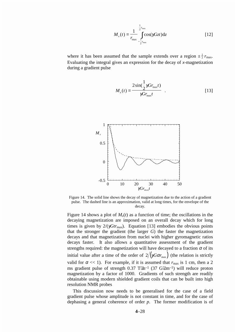
Figure 14. The solid line shows the decay of magnetization due to the action of a gradient pulse. The dashed line is an approximation, valid at long times, for the envelope of the

decay.

Figure 14 shows a plot of Mx(t) as a function of time; the oscillations in the decaying magnetization are imposed on an overall decay which for long times is given by 2/(γGtrmax). Equation [13] embodies the obvious points that the stronger the gradient (the larger G) the faster the magnetization decays and that magnetization from nuclei with higher gyromagnetic ratios decays faster. It also allows a quantitative assessment of the gradient strengths required: the magnetization will have decayed to a fraction α of its

initial value after a time of the order of ( )2 γ αG rmax (the relation is strictly

valid for α << 1). For example, if it is assumed that rmax is 1 cm, then a 2 ms gradient pulse of strength 0.37 T⋅m–1 (37 G⋅cm–1) will reduce proton magnetization by a factor of 1000. Gradients of such strength are readily obtainable using modern shielded gradient coils that can be built into high resolution NMR probes This discussion now needs to be generalised for the case of a field gradient pulse whose amplitude is not constant in time, and for the case of dephasing a general coherence of order p. The former modification is of

4–29

importance as for instrumental reasons the amplitude envelope of the gradient is often shaped to a smooth function. In general after applying a gradient pulse of duration τ the spatially dependent phase, Φ(r,τ) is given by

Φ( , ) ( )r sp B rgτ γ τ= [14]

The proportionality to the coherence order comes about due to the fact that the phase acquired as a result of a z-rotation of a coherence of order p through an angle φ is pφ, (see Eqn. [1] in section 4.2.4.1). In Eqn. [14] s is a shape factor: if the envelope of the gradient pulse is defined by the

function A(t), where A t( ) ≤ 1, s is defined as the area under A(t)

s = 1τ

A t( )0

τ

∫ dt

. [15]

The shape factor takes a particular value for a certain shape of gradient, regardless of its duration. A gradient applied in the opposite sense, that is with the magnetic field decreasing as the z-coordinate increases rather than vice versa, is described by reversing the sign of s. The overall amplitude of the gradient is encoded within Bg. In the case that the coherence involves more than one nuclear species, Eqn. [14] is modified to take account of the different gyromagnetic ratio for each spin, γi, and the (possibly) different order of coherence with respect to each nuclear species, pi:

Φ( , ) ( )r sB r pg i ii

τ τ γ= ∑ . [16]

From now on we take the dependence of Φ on r and t, and of Bg on r as being implicit, and will not write these explicitly.

4.3.2.2 Selection by Refocusing

The method by which a particular coherence transfer pathway is selected using field gradients is illustrated in Fig.15 (a).

4–30

RF

(a)

g τ 1 τ 2

p1

p2

RF

(b)

g τ 1 τ 2

p 12

0–1–2

τ 3 τ 4

Figure 15 Pulse sequences and associated coherence transfer pathways illustrating coherence selection using gradients. The radiofrequency pulses are given on the line

marked RF, solid rectangles indicate 90° pulses and open rectangles indicate 180° pulses; the pulse phase is x unless otherwise specified. Gradient pulses are indicated by the

rectangles on the line marked g.

The first gradient pulse encodes a spatially dependent phase, Φ1 and the second a phase Φ2 where

Φ Φ1 1 1 1 2 2 2 2= =s p B s p Bg,1 g,2andτ τ

. [17]

After the second gradient the net phase is (Φ1 + Φ2). To select the pathway involving transfer from coherence order p1 to coherence order p2, this net phase should be zero; in other words the dephasing induced by the first gradient pulse is undone by the second. The condition (Φ1 + Φ2) = 0 can be rearranged to

s B

s B

p

p1 1

2 2

2

1

g,1

g,2

ττ

=–

. [18]

For example, if p1 = +2 and p2 = – 1, refocusing can be achieved by making the second gradient either twice as long (τ2 = 2 τ1), or twice as strong (Bg,2 = 2 Bg,1) as the first; this assumes that the two gradients have identical shape factors. Other pathways remain dephased; for example, assuming that we have chosen to make the second gradient twice as strong and the same duration as the first, a pathway with p1 = +3 to p2 = –1 experiences a net phase

Φ Φ1 2 1 2 1 13+ = =sB sp B sBg,1 g,2 g,1τ τ τ–

. [19]

Provided that this spatially dependent phase is sufficiently large, according the criteria set out in the previous section, the coherence arising from this pathway remains dephased and is not observed. To refocus a pathway in which there is no sign change in the coherence orders, for example, p1 = – 2 to p2 = – 1, the second gradient needs to be applied in the opposite sense to the first; in terms of Eqn. [18] this is expressed by having s2 = – s1.

4–31

The procedure can easily be extended to select a more complex coherence transfer pathway by applying further gradient pulses as the coherence is transferred by further pulses, as illustrated in Fig. 15 (b). The condition for refocusing is again that the net phase acquired by the required pathway be zero, which can be written formally as

s p Bi i i

ig,iτ∑ = 0

. [20]

With more than two gradients there are many ways in which a given pathway can be selected. For example, the second gradient may be used to refocus the first part of the required pathway, leaving the third and fourth to refocus another part. Alternatively, the pathway may be consistently dephased and the magnetization only refocused by the final gradient, just before acquisition. At this point it is useful to contrast the selection achieved using gradient pulses with that achieved using phase cycling. From Eqn. [18] it is clear that a particular pair of gradient pulses selects a particular ratio of coherence orders; in the above example any two coherence orders in the ratio –2 : 1 or 2 : – 1 will be refocused. This selection according to ratio is in contrast to the case of phase cycling in which a phase cycle consisting of N steps of 2π /N radians selects a particular change in coherence order ∆p = p2 – p1, and further pathways which have ∆p = (p2 – p1) ± mN, where m = 0, 1, 2 ... It is straightforward to devise a series of gradient pulses which will select a single coherence transfer pathway. It cannot be assumed, however, that such a sequence of gradient pulses will reject all other pathways i.e. leave coherence from all other pathways dephased at the end of the sequence. Such assurance can only be given be analysing the fate of all other possible coherence transfer pathways under the particular gradient sequence proposed. In complex pulse sequences there may also be several different ways in which gradient pulses can be included in order to achieve selection of the desired pathway. Assessing which of these alternatives is the best, in the light of the requirement of suppression of unwanted pathways and the effects of pulse imperfections may be a complex task. In this section it has been shown that a single coherence transfer pathway can be selected with the aid of gradient pulses. However, it is not unusual to want to select two or more pathways simultaneously. A good example of this is the double-quantum filter pulse sequence element shown in Fig. 16 (a).

12

0–1–2

RF

p

(a)

g

(b)

RF RF

(c)

g

12

0–1–2

12

0–1–2

4–32

Figure 16 Pulse sequences and pathways for double-quantum filters.

The ideal pathway, shown in (a), preserves coherence orders p = ± 2 during the inter-pulse delay. It can be shown that the first 90° pulse generates equal amounts of coherence orders + 2 and – 2, and these contribute equally to the final observable signal. Gradients can be used to select the pathway – 2 to – 1 or + 2 to – 1, shown in (b) and (c) respectively. However, no combination of gradients can be found which will select simultaneously both of these pathways. In contrast, it is easy to devise a phase cycle which selects both of these pathways (section 4.2.6.2). Thus, selection with gradients will in this case result in a loss of half of the available signal when compared to an experiment of equal length which uses selection by phase cycling. Such a loss in signal is, unfortunately, a very common feature when gradients are used for pathway selection. Coherence order zero, comprising z-magnetization, zz terms and homonuclear zero-quantum coherence, does not accrue any phase during a gradient pulse. Thus it can be separated from all other orders simply by applying a single gradient. In a sense, however, this is not a gradient selection process; rather it is a simply suppression of all other coherences. In contrast to experiments where selection is achieved, there is no inherent sensitivity loss. The simplest experimental arrangement generates a gradient in which the magnetic field varies in the z direction, however it is also possible to generate gradients in which the field varies along x or y. Clearly, the spatially dependent phase generated by a gradient applied in one direction cannot be refocused by a gradient applied in a different direction. In sequences where more than one pair of gradients are used, it may be convenient to apply further gradients in different directions to the first pair, so as to avoid the possibility of accidentally refocusing unwanted coherence transfer pathways. Likewise, a gradient which is used to destroy all magnetization and coherences can be applied in a different direction to gradients subsequently used for pathway selection.

4.3.2.3 Spin Echoes

Refocusing pulses play an important role in multiple-pulse NMR experiments and so the interaction between such pulses and field gradient pulses will be explored in some detail. A perfect refocusing pulse achieves two effects. Firstly, it changes the sign of the order of any coherences present, p → – p. Secondly, z-magnetization is inverted Iz → – Iz. A perfect 180° pulse, applied about any axis, is an example of such a refocusing pulse. An imperfect refocusing pulse will cause transfers to other coherence orders than – p, and may generate transverse magnetization from any z-magnetization present. We start out the discussion by considering the refocusing of coherences.

4–33

RF

p

(a)

g

(c)δ δ

ττ

–p

RF

(b)

g

δ δ

ττ

g

δ δ

ττ

I

S

RF

(d)

g ττ

τ z

+10

–1p

RF

(e)

g τ

RF

(f)

g

τ/2τ/2

τ

Figure 17 Spin echoes and related sequences. In heteronuclear experiments the radiofrequency pulses applied to the I and S spins are indicated on the lines so marked

The effect of an imperfect refocusing pulse can be considered by factoring the sample into a part which experiences perfect refocusing and a part which does not. The refocused part can be selected by placing a gradient pulse on either side of the refocusing pulse, as shown in Fig. 17 (a). The net phase at the end of such a sequence is

( )Φ Ω Ω2τ δ γ τ δ γ τ= + + +( ) ( ') 'p psp B sp Bg g [21]

where Ω(p) is the frequency with which coherence of order p evolves in the absence of a gradient; note that Ω(–p) = – Ω(p). This net phase is zero if, and only if, p' = – p. With sufficiently strong gradients all other pathways remain dephased and the gradient sequence has thus selected the perfectly refocused component. In addition, any transverse magnetization created by an imperfect refocusing pulse is also dephased. As is expected for a spin echo, the underlying evolution of the coherence (as would occur in the absence of a gradient) for the entire time 2δ is also refocused. If a refocusing pulse is used in its second context, that of inversion of z magnetization, the considerations are somewhat different. Formally, we could regard the problem as selecting the pathway p = 0 → p' = 0, in which case any combination of gradients would be suitable. However, in practice a gradient combination should be used which gives the maximum dephasing effect to other coherences. Assuming that the refocusing pulse still changes the sign of the larger fraction of the coherences in the sample, the greatest dephasing is obtained when the second gradient is applied in the opposite sense to the first, as is shown in Fig. 17 (b). In heteronuclear experiments a refocusing pulse is often used to remove the effects of the heteronuclear coupling over a period. The role of such a

4–34

pulse when applied to spins S is simply to invert the sign of any operator products involving Sz; in other words to act as an inversion pulse for S. This function is selected using the gradient sequence shown in Fig. 17 (c), which in analogous to (b). Of course, any coherences on the spins I will be dephased by the first gradient, but these coherences will be rephased by the second gradient as it is applied in the opposite sense. The net effect is that the I spin shift evolves for 2δ, but the IS coupling is refocused. If a refocusing pulse is perfect, the inclusion of gradient pulses as shown in Fig. 17 (a) - (c) does not reduce the size of the ultimately observed signal. This is in contrast to most other situations in which selection with gradients results in an inherent loss of signal. However, if the refocusing pulse is imperfect there will be a loss of signal reflecting that part of the sample which does not experience a perfect refocusing pulse.

4.3.2.4 Phase Errors

In the selection process the spatially dependent phase created by a gradient pulse is subsequently refocused by a second gradient pulse. However, the underlying evolution due to chemical shifts (offsets) and couplings is not refocused, and phase errors will accumulate due to the evolution of these terms. Since gradient pulses are typically of a few milliseconds duration, these phase errors are far from insignificant.

12

0–1–2

RF

g τ 1 τ 2

t1 t2

p

Figure 18. A DQF COSY sequence with gradient selection.

In multi-dimensional NMR the uncompensated evolution of offsets during gradient pulses has disastrous effects on the spectra. This is illustrated here for the double-quantum filtered COSY pulse sequence using the gradient pulses shown in Fig. 18. It will be assumed that only the indicated pathway survives and so the spatially dependent part of the evolution due to the gradients will be ignored. Thus, for a two spin system, coherence order of + 2 present during the filter evolves as follows during the first gradient pulse

( )( )I I I I iI Iz z

1 2 1 2 1 2 11 1 1 2 1 2

+ ++

+ + → +Ω Ω Ω Ωτ τ τexp – , [22]

where Ω1 and Ω2 are the offsets of spins 1 and 2, respectively. After the

4–35

final 90° pulse and the second gradient the observable terms on spin 1 are

( )( )[ ]i

x z y zi I I I I2 1 2 1 1 2 1 2 1 2 1 22 2exp – cos sinΩ Ω Ω Ω+ +τ τ τ [23]

where it has been assumed that τ2 is sufficiently short that evolution of the coupling can be ignored. It is clearly seen from Eqn. [23] that, due to the evolution during τ2, the multiplet observed in the F2 dimension will be a mixture of dispersion and absorption anti-phase contributions. In addition, the exponential term gives an overall phase shift due to the evolution during τ1. The phase correction needed to restore this multiplet to absorption depends on both the frequency in F2 and the double-quantum frequency during the first gradient. Thus, no single linear frequency dependent phase correction could phase correct a spectrum containing many multiplets. The need to control these phase errors is plain. The general way to minimise these problems is to associate each gradient pulse with a refocusing pulse as shown in Fig. 17 (e) and (f). Using the results from the previous section it is easily seen that sequence (e) generates a net phase of spγBgτ; (f) gives the same result with a sign change. The desired effect of refocusing the evolution due to the offset and not that due to the gradient has been achieved. In sequence (f) the gradient is split into two halves by the refocusing pulse, and in order to avoid the second gradient refocusing the effect of the first, the two gradients have to be applied in opposite senses. Of these two options (f) is the most time efficient as the gradient is applied for the entire duration, whereas option (e) lengthens the experiment by doubling the time needed for each gradient; if relaxation is rapid, option (f) is the method of choice. As was explained in the previous section, if the refocusing pulse is imperfect coherences undergoing transfers other than the required p → – p should be dephased by (f). However, sequence (e) will dephase the results of only some of these unwanted coherence transfers. In many pulse sequences there are periods during which the evolution of offsets is refocused. The evolution of offsets during a gradient pulse placed within such a period will therefore also be refocused, making it unnecessary to include extra refocusing pulses. Likewise, a gradient may be placed during a "constant time" evolution period of a multi-dimensional pulse sequence without introducing phase errors in the corresponding dimension; the gradient simply becomes part of the constant time period. This approach is especially useful in the constant time three- and four-dimensional experiments used to record spectra of nitrogen-15, carbon-13 labelled proteins.

4.3.3 Lineshapes in Multi-Dimensional Spectra

The use of gradient pulses during the incremented time of a multi-dimensional NMR experiment has profound effects on the lineshapes in the resulting spectrum . To illustrate this we will discuss the simple COSY experiment and restrict ourselves to a single spin with offset Ω. The principles remain the same for more complex experiments.

4–36

10

–1

RF

p

10

–1

RF

g

(a) (b) t1 t2 t1 t2

p

Figure 19. Pulse sequences for COSY, with and without gradient selection.

Figure 19 (a) shows the basic COSY pulse sequence; a simple analysis of this sequence for a one line spectrum gives the observed signal Sc(t1,t2) as

( ) ( ) ( ) ( )S t t t t T i t t Tc 1 2 1 1 2 2 2 2, cos exp – / exp exp – /= Ω Ω [24]

where T2 is the (assumed) transverse relaxation time of the spin and quadrature detection in t2 is also assumed. The crucial feature of this signal is that it is cosine modulated in t1 and since cos(Ωt1) = cos(–Ωt1), the modulation of the signal in t1 is invariant to the sign of the offset, Ω. As a result the spectrum is said to lack frequency discrimination in the F1 dimension. Since the receiver reference is normally placed in the middle of the spectrum, resonances will have both positive and negative offsets, but these are not distinguished in the F1 dimension leading to a confused and overlapped spectrum. All methods of achieving frequency discrimination are based on recording a separate signal, Ss, which is sine modulated in t1. In the COSY experiment this signal is achieved simply by changing the phase of the first pulse by 90°, giving

( ) ( ) ( ) ( )S t t t t T i t t Ts 1 2 1 1 2 2 2 2, sin exp – / exp exp – /= Ω Ω . [25]

The way in which Sc and Ss are used to generate a frequency discriminated spectrum is as follows. The real and imaginary parts of the Fourier transform of this exponentially damped signal are lines with the absorption and dispersion lorentzian lineshapes, denoted A(ω) and D(ω) respectively

( ) ( )[ ] ( ) ( )F exp exp – /± = +± ±i t t T A iDΩ 2 2 2 ω ω [26]

( )

( )( ) ( )

( )where ,AT

TD

T

T± ±=+

=+

ωω

ωωω

22

22

22

2221 1

ΩΩΩ , [27]

4–37

and F[S(t)] denotes the Fourier transform of S(t). Thus the transforms with respect to t2 of Sc and Ss are

( ) ( )[ ] ( ) ( ) ( ) S t S t t t t T A iDc c1 2 1 2 1 1 2 2 2, , cos exp – /ω ω ω= F2 = ++ +Ω [28]

( ) ( )[ ] ( ) ( ) ( ) S t S t t t t T A iDs s1 2 1 2 1 1 2 2 2, , sin exp – /ω ω ω= F2 = ++ +Ω .[29]

The real part of Sc(t1,ω2) is combined with i times the real part of Ss(t1,ω2) to yield the signal S(t1,ω2) whose transform is the required spectrum

( ) ( )[ ] ( )[ ]( ) ( ) ( )

S t S t i S t

i t t T A

1 2 1 2 1 2

1 1 2 2

, Re , Re ,

exp exp – /

ω ω ω

ω

= +

= +

c s

Ω [30]

( ) ( )[ ] ( ) ( ) ( )S S t A iD Aω ω ω ω ω ω1 2 1 2 1 1 2, ,= F1 = ++ + + . [31]

The real part of S(ω1,ω2) is a spectrum with the favourable double absorption lineshape, A+(ω1)A+(ω2). In addition, inspection of Eqn. [30] shows that the spectrum is frequency discriminated as the modulation in t1 is sensitive to the sign of Ω. This process of forming an absorption mode, frequency discriminated spectrum is just that due to States, Haberkorn and Ruben (SHR). A closely related process, knows as the Marion-Wüthrich or TPPI method, achieves the same result by incrementing the phase of the first pulse by 90° each time that t1 is incremented. It can be shown that provided the increment of t1 is half that in the SHR method, an identical frequency discriminated double absorption spectrum results. There are two possible ways, shown in Fig. 19 (b), of using gradients in the COSY sequence. Either coherence level + 1 is selected during t1, leading to the echo or N-type spectrum, or level – 1 is selected leading to the anti-echo or P-type spectrum. As has been pointed out, it is not possible to select simultaneously both of these pathways. The time domain signals for the P- and N-type pathways are

( ) ( ) ( ) ( )S t t i t t T i t t TP ( , ) exp exp exp exp1 212 1 1 2 2 2 2= − −Ω Ω [32]

( ) ( ) ( ) ( )S t t i t t T i t t TN ( , ) exp exp exp exp1 212 1 1 2 2 2 2= − − −Ω Ω [33]

In each case the resulting spectrum is expected to be frequency discriminated due to the complex exponential modulation in t1; the factor of

4–38

one half arises because the magnetization generated at the start of t1 is an equal mixture of coherence orders + 1 and – 1, only one of which is refocused by the final field gradient. The use of gradient pulses has resulted in frequency discrimination without any further data processing or without the need to acquire further data sets with phase shifted pulses. This is a consequence of selecting just one coherence level during t1. Double Fourier transformation of SP and SN gives the spectra

( ) ( ) ( ) ( ) ( ) ( ) ( ) ( ) ( )

S A A D D

A D D A

P

i

ω ω ω ω ω ω

ω ω ω ω

1 212 1 2 1 2

2 1 2 1 2

, = −

+ +

+ + + +

+ + + + [34]

( ) ( ) ( ) ( ) ( ) ( ) ( ) ( ) ( )

S A A D D

A D D A

N

i

ω ω ω ω ω ω

ω ω ω ω

1 212 1 2 1 2

2 1 2 1 2

, = −

+ +

− + − +

− + − + [35]

4–39

Figure 20 Experimental spectra showing how P-type and an axis-reversed N-type spectrum, each of which has the phase-twist lineshape, can be added together to give an absorption

mode spectrum.

In each case the real part of the spectrum has the phase-twist lineshape,

( ) ( ) ( ) ( ) A A D D± + ± +−ω ω ω ω1 2 1 2 , which is an inextricable mixture of

absorption and dispersion. This lineshape is very undesirable in high

4–40

resolution NMR both because it is broad and because it has positive and negative parts. Unless further steps are taken, applying a gradient during t1 will always result in a phase-twist lineshape. When gradients have been applied during t1 an absorption mode spectrum can be recovered by repeating the experiment twice, once to give the P-type and once to give the N-type spectrum. Figure 20 shows typical P- and N-type spectra recorded using gradient pulse selection. If the F1 axis of the N-type spectrum is reversed the result is identical to the P-type spectrum except that the dispersive part of the phase twist is in the opposite sense. Adding the axis-reversed N-type and P-type spectra together cancels the dispersive parts of the phase twist, leaving a peak with a double absorption lineshape.

This process is conveniently carried out in the following way. The data from the P- and N-type spectra are transformed with respect to t2 to give

S t i t t T A iDP ( , ) exp( ) exp( / ) ( ) ( )1 2 1 1 2 2 2

1

2ω ω ω= − ++ +Ω [36]

S t i t t T A iDN ( , ) exp( ) exp( / ) ( ) ( )1 2 1 1 2 2 2

1

2ω ω ω= − − ++ +Ω [37]

These are combined to give the new signal S+(t1,ω2) according to

S t S t S t

i t t T AP N

+ ∗

+

= += −

( , ) ( , ) ( , )

exp( ) exp( / ) ( )1 2 1 2 1

1 1 2 2

ω ω ωωΩ

[38]

Taking the complex conjugate of the time domain signal is equivalent to reversing the corresponding frequency axis in the frequency domain. Finally, Fourier transformation with respect to t1 yields, in the real part, the required double absorption lineshape

S A iD A++ + += +( , ) ( ) ( ) ( )ω ω ω ω ω1 2 1 1 2 . [39]

If the software available is not capable of the manipulations described above, the cosine and sine modulated data sets needed for conventional SHR type processing can be generated by manipulating the P- and N-type time domain data in the following way. The P- and N-type data sets are stored separately; adding them together produces a cosine modulated data set, whereas subtracting them from one another produces a sine modulated data set. These statements can be demonstrated by considering the sum and difference of the functions SP(t1,t2) and SN(t1,t2) (Eqns. [32] and [33] respectively) together with the well known identities 2 cosθ = exp(iθ) + exp(–iθ) and 2i sinθ = exp(iθ) – exp(–iθ). In the presence of significant inhomogeneous broadening P- and N-type spectra have different lineshapes. The most convenient way to understand

4–41

this is to imagine that the sample is divided into small compartments, in each of which the B0 field is sufficiently homogeneous that the natural linewidth dominates. Each compartment contributes a phase-twist line to the spectrum, at a frequency determined by the precise value of the B0 field in that compartment. These phase-twist lines from different compartments will overlap with one another and may cancel or reinforce, depending on how they are distributed. In the N-type spectrum the phase-twists lines are so arranged that they reinforce one another, giving, in the limit of a wide distribution of frequencies, a largely positive ridge-like lineshape. In contrast, in the P-type spectrum the phase-twists are aligned in such a way that they cancel one another. In the limit of a wide distribution, the cancellation is all but complete. This strong asymmetry has led some to conclude that frequency discrimination methods based on combining P- and N-type spectra would be rendered ineffective by the presence of inhomogeneous broadening. However, this view is mistaken as the following argument reveals. Each compartment gives a P- and an N-type spectra with identical peak heights. Thus, when the spectra are combined, these individual phase-twists add together in precisely the way required, cancelling the dispersion contributions. The observed spectrum is the sum of these individual spectra, thus the dispersive contributions are removed from it as well.

4.3.4 Sensitivity

The use of gradients for coherence selection has consequences for the signal-to-noise ratio of the resulting spectrum when it is compared to a similar spectrum recorded using phase cycling. Most of the differences between the sensitivity of the gradient and phase cycled experiments come about because a gradient is only capable of selecting one coherence order at a particular point in the sequence. In contrast, it is often possible to select more than one coherence order when phase cycling is used (see section 4.3.2.2). If a gradient is used to suppress all coherences other than p = 0, i.e. it is used simply to remove all coherences, leaving just z-magnetization or zz terms, there is no inherent loss of sensitivity when compared to a corresponding phase cycled experiment. If, however, the gradient is used to select a particular order of coherence the signal which is subsequently refocused will almost always be half the intensity of that which can be observed in a phase cycled experiment. This factor comes about simply because it is likely that the phase cycled experiment will be able to retain two symmetrical pathways, whereas the gradient selection method will only be able to refocuse one of these. The foregoing discussion applies to the case of a selection gradient placed in a fixed delay of a pulse sequence. The matter is quite different if the gradient is placed within the incrementable time of a multi-dimensional experiment, e.g. in t1 of a two-dimensional experiment. To understand the effect that such a gradient has on the sensitivity of the experiment it is necessary to be rather careful in making the comparison between the gradient selected and phase cycled experiments. In the case of the latter experiments we need to include the SHR or TPPI method in order to achieve frequency discrimination with absorption mode lineshapes. If a gradient is

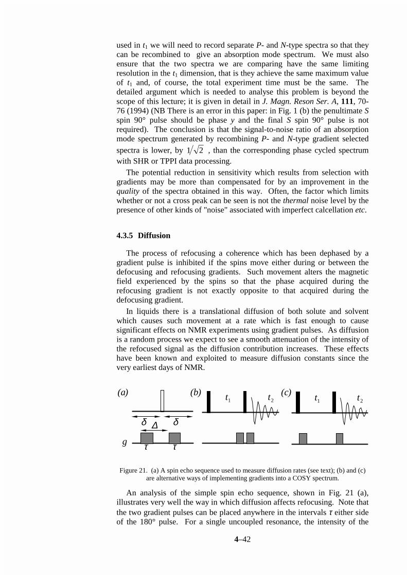
4–42

used in t1 we will need to record separate P- and N-type spectra so that they can be recombined to give an absorption mode spectrum. We must also ensure that the two spectra we are comparing have the same limiting resolution in the t1 dimension, that is they achieve the same maximum value of t1 and, of course, the total experiment time must be the same. The detailed argument which is needed to analyse this problem is beyond the scope of this lecture; it is given in detail in J. Magn. Reson Ser. A, 111, 70-76 (1994) (NB There is an error in this paper: in Fig. 1 (b) the penultimate S spin 90° pulse should be phase y and the final S spin 90° pulse is not required). The conclusion is that the signal-to-noise ratio of an absorption mode spectrum generated by recombining P- and N-type gradient selected

spectra is lower, by 1 2 , than the corresponding phase cycled spectrum with SHR or TPPI data processing. The potential reduction in sensitivity which results from selection with gradients may be more than compensated for by an improvement in the quality of the spectra obtained in this way. Often, the factor which limits whether or not a cross peak can be seen is not the thermal noise level by the presence of other kinds of "noise" associated with imperfect calcellation etc.

4.3.5 Diffusion

The process of refocusing a coherence which has been dephased by a gradient pulse is inhibited if the spins move either during or between the defocusing and refocusing gradients. Such movement alters the magnetic field experienced by the spins so that the phase acquired during the refocusing gradient is not exactly opposite to that acquired during the defocusing gradient. In liquids there is a translational diffusion of both solute and solvent which causes such movement at a rate which is fast enough to cause significant effects on NMR experiments using gradient pulses. As diffusion is a random process we expect to see a smooth attenuation of the intensity of the refocused signal as the diffusion contribution increases. These effects have been known and exploited to measure diffusion constants since the very earliest days of NMR.

(a)

g

δ δ ∆

(b) t1 t2

(c) t1 t2

τ τ

Figure 21. (a) A spin echo sequence used to measure diffusion rates (see text); (b) and (c) are alternative ways of implementing gradients into a COSY spectrum.

An analysis of the simple spin echo sequence, shown in Fig. 21 (a), illustrates very well the way in which diffusion affects refocusing. Note that the two gradient pulses can be placed anywhere in the intervals τ either side of the 180° pulse. For a single uncoupled resonance, the intensity of the

4–43

observed signal, S, expressed as a fraction of the signal intensity in the absence of a gradient, S0 is given by

S

SG D

0

2 2 2

3= − −

exp γ ττ

∆ [40]

where D is the diffusion constant, ∆ is the time between the start of the two gradient pulses and τ is the duration of the gradient pulses; relaxation has been ignored. For a given pair of gradient pulses it is diffusion during the interval between the two pulses, ∆, which determines the attenuation of the echo. The gradients are used to label the magnetization with a spatially dependent phase, and then to refocus it. The stronger the gradient the more rapidly the phase varies across the sample and thus the more rapidly the echo will be attenuated. This is the physical interpretation of the term γ2G2τ2 in Eqn. [40]. Diffusion constants generally decrease as the molecular mass increases. A small molecule, such as water, will diffuse up to twenty times faster than a protein with molecular weight 20,000. Table 1 shows the loss in intensity due to diffusion for typical gradient pulse pair of 2 ms duration and of strength 10 G⋅cm–1 for a small, medium and large sized molecule; data is given for ∆ = 2 ms and ∆ = 100 ms. It is seen that even for the most rapidly diffusing molecules the loss of intensity is rather small for ∆ = 2 ms, but becomes significant for longer delays. For large molecules, the effect is small in all cases.

Table I : Fraction of Transverse Magnetization Refocused

After a Spin Echo with Gradient Refocusinga

∆/msb small moleculec medium sized moleculed

macro moleculee

2 0.99 1.00 1.00 100 0.55 0.88 0.97

a Calculated for the pulse sequence of Fig. 21 (a) for two gradients of

strength

10 G⋅cm–1 and duration, τ, 2 ms; relaxation is ignored.

b As defined in Fig. 21 (a).

c Diffusion constant, D, taken as that for water, which is 2.1 × 10–9 m2 s–1 at

ambient temperatures.

d Diffusion constant taken as 0.46 × 10–9 m2 s–1.

e Diffusion constant taken as 0.12 × 10–9 m2 s–1.

4–44

4.3.5.1 Minimisation of Diffusion Losses

The foregoing discussion makes it clear that in order to minimise intensity losses due to diffusion the product of the strength and durations of the gradient pulses, G2τ2, should be kept as small as is consistent with achieving the required level of suppression. In addition, a gradient pulse pair should be separated by the shortest time within the limits imposed by the pulse sequence. This condition applies to gradient pairs the first of which is responsible for dephasing, and the second for rephasing. Once the coherence is rephased the time that elapses before further gradient pairs is irrelevant from the point of view of diffusion losses. In two-dimensional NMR diffusion can lead to line broadening in the F1 dimension if t1 intervenes between a gradient pair. Consider the two alternative pulse sequences for recording a simple N-type COSY spectrum shown in Fig. 21 (b) and (c). In (b) the gradient pair are separated by the very short time of the final pulse, thus keeping the diffusion induced losses to an absolute minimum. In (c) the two gradients are separated by the incrementable time t1; as this increases the losses due to diffusion will also increase resulting in an extra decay of the signal in t1. The extra line broadening due to this decay can be estimated from Eqn. [40], with ∆ = t1, as γ2G2τ2D/π Hz. For a pair of 2 ms gradients of strength 10 G⋅cm–1 this amounts This effect by which diffusion causes an extra line broadening in the F1 dimension is usually described as diffusion weighting. Generally it is possible to avoid this effect by careful placing of the gradients. For example, the sequences in Fig. 21 (b) and (c) are in every other respect equivalent, thus there is no reason not to chose (b). It should be emphasised that diffusion weighting occurs only when t1 intervenes between the dephasing and refocusing gradients.

4.3.6 Some Examples of Experiments Using Gradients

4.3.6.1 General Remarks

Reference has already been made to the two general advantages of using gradient pulses for coherence selection, namely the possibility of a general improvement in the quality of spectra and the removal of the requirement of completing a phase cycle for each increment of a multi-dimensional experiment. In the case of recording spectra of proteins and similar molecules a number of particular advantages can be expected. The first of these relates to heteronuclear correlation experiments which form the heart of many two- and higher-dimensional experiments. In such experiments there is a need to suppress both the water resonance and the signals due to protons not coupled to a heteronucleus (nitrogen-15 or carbon-13, typically); selection with gradients will give improve greatly the suppression of both these types of signals. Finally, we note that the dynamic range of the free induction decay recorded after gradient selection will be much lower than in an equivalent phase cycled experiment, allowing best use to be made of the resolution of the digitiser. As has been discussed above, special care needs to be taken in

4–45

experiments which use gradient selection if absorption mode spectra are to be obtained. For demanding applications where spectral resolution and sensitivity is at a premium, it is vital to record absorption mode spectra. This is especially the case in the indirectly detected domains of two- and higher-dimensional spectra. In the following sections the use of gradient selection in several different experiments will be described. The gradient pulses used in these sequences will be denoted G1, G2 etc. where Gi implies a gradient of duration τi, strength Bg,i and shape factor si. There is always the choice of altering the duration, strength or, conceivably, shape factor in order to establish refocusing. Thus, for brevity we shall from now on write the spatially dependent phase produced by gradient Gi acting on coherence of order p as pGi in the homonuclear or γ j j i

j

p G∑ in the heteronuclear case.

4.3.6.2 Double Quantum Filtered COSY

12

0–1–2

RF

g

t1 t2

p

G2G1

Figure 22. Pulse sequence for recording absorption mode DQF COSY spectra.

The sequence of Fig. 22 is suitable for recording absorption mode DQF COSY spectrum. Here, no gradient is applied during t1, thus retaining symmetrical pathways and the phase errors which accumulate during the double quantum period are refocused by an extra 180° pulse; the refocusing condition is G2 = 2 G1. Frequency discrimination in the F1 dimension is achieved by the SHR or TPPI procedures. Multiple quantum filters through higher orders can be implemented in the same manner. In this experiment data acquisition is started immediately after the final radiofrequency pulse so as to avoid phase errors which would accumulate during the second gradient pulse. Of course, the signal only rephases towards the end of the final gradient, so there is little signal to be observed. However, the crucial point is that, as the magnetization is all in antiphase at the start of t2, the signal grows from zero at a rate determined by the size the couplings on the spectrum. Provided that the gradient pulse is much shorter that 1/J, where J is a typical proton-proton coupling constant, the part of the signal missed during the gradient pulse is not significant and the spectrum is not perturbed. Acquiring the data in this way avoids the need for an extra

4–46

180° pulse to refocus the phase errors that would accumulate during the second gradient. If it is more convenient, an alternative procedure is to start to acquire the data after the final gradient, and then to right shift the free induction decay, bringing in zeroes from the left, by a time equal to the duration of the gradient.

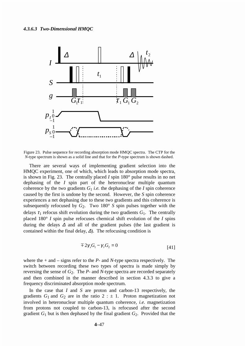
4–47

4.3.6.3 Two-Dimensional HMQC

g

I

S t1

t2∆ ∆

τ 1 τ 1G1 G1 G2

10

–1 pI

10

–1 pS

Figure 23. Pulse sequence for recording absorption mode HMQC spectra. The CTP for the N-type spectrum is shown as a solid line and that for the P-type spectrum is shown dashed.

There are several ways of implementing gradient selection into the HMQC experiment, one of which, which leads to absorption mode spectra, is shown in Fig. 23. The centrally placed I spin 180° pulse results in no net dephasing of the I spin part of the heteronuclear multiple quantum coherence by the two gradients G1 i.e. the dephasing of the I spin coherence caused by the first is undone by the second. However, the S spin coherence experiences a net dephasing due to these two gradients and this coherence is subsequently refocused by G2. Two 180° S spin pulses together with the delays τ1 refocus shift evolution during the two gradients G1. The centrally placed 180° I spin pulse refocuses chemical shift evolution of the I spins during the delays ∆ and all of the gradient pulses (the last gradient is contained within the final delay, ∆). The refocusing condition is

2 01 2γ γs IG G− = [41]

where the + and – signs refer to the P- and N-type spectra respectively. The switch between recording these two types of spectra is made simply by reversing the sense of G2. The P- and N-type spectra are recorded separately and then combined in the manner described in section 4.3.3 to give a frequency discriminated absorption mode spectrum. In the case that I and S are proton and carbon-13 respectively, the gradients G1 and G2 are in the ratio 2 : ± 1. Proton magnetization not involved in heteronuclear multiple quantum coherence, i.e. magnetization from protons not coupled to carbon-13, is refocused after the second gradient G1 but is then dephased by the final gradient G2. Provided that the

4–48

gradient is strong enough these unwanted signals, and the t1-noise associated with them, will be suppressed.

4–49

4.3.6.4 Two-Dimensional HSQC

(a)

(b)

g

I

S t1

t2∆ ∆ ∆∆

y

a

I

S t1

t2∆ ∆ ∆∆

τ 110

–1 pI

10

–1 pS

G1 G2

Figure 24. Pulse sequences for recording absorption mode HSQC spectra: (a) is the usual sequence, see text for a description of the significance of point a; (b) gives P- or N-type

spectra which can be recombined to give an absorption mode spectrum.

The basic pulse sequence for the HSQC experiment is shown in Fig. 24 (a). For a coupled two spin system the transfer can be described as proceeding via the spin ordered state 2IzSz which exists at point a in the sequence. In the absence of significant relaxation magnetization from uncoupled I spins is present at this point as Iy. Thus, a field gradient applied at point a will dephase the unwanted magnetization and leave the wanted term unaffected. The main practical difficulty with this approach is that the uncoupled magnetization is only along y at point a provided all of the pulses are perfect; if the pulses are imperfect there will be some z magnetization present which will not be eliminated by the gradient. In the case of observing proton - carbon-13 or proton - nitrogen-15 HSQC spectra from natural abundance samples, the magnetization from uncoupled protons is very much larger than the wanted magnetization, so even very small imperfections in the pulses can give rise to unacceptably large residual signals. However, for globally labelled samples the degree of suppression has been shown to be sufficient, especially if some minimal phase cycling or other procedures are used in addition. Indeed, such an approach has been

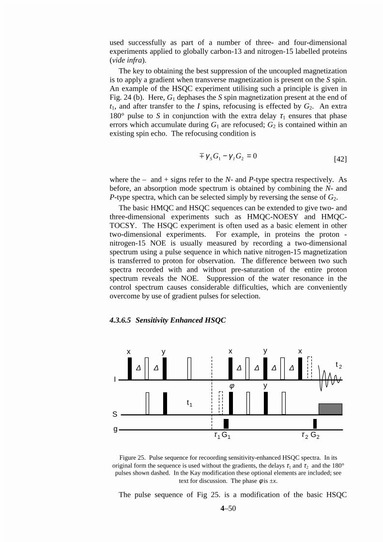
4–50

used successfully as part of a number of three- and four-dimensional experiments applied to globally carbon-13 and nitrogen-15 labelled proteins (vide infra). The key to obtaining the best suppression of the uncoupled magnetization is to apply a gradient when transverse magnetization is present on the S spin. An example of the HSQC experiment utilising such a principle is given in Fig. 24 (b). Here, G1 dephases the S spin magnetization present at the end of t1, and after transfer to the I spins, refocusing is effected by G2. An extra 180° pulse to S in conjunction with the extra delay τ1 ensures that phase errors which accumulate during G1 are refocused; G2 is contained within an existing spin echo. The refocusing condition is

γ γS IG G1 2 0− = [42]

where the – and + signs refer to the N- and P-type spectra respectively. As before, an absorption mode spectrum is obtained by combining the N- and P-type spectra, which can be selected simply by reversing the sense of G2. The basic HMQC and HSQC sequences can be extended to give two- and three-dimensional experiments such as HMQC-NOESY and HMQC-TOCSY. The HSQC experiment is often used as a basic element in other two-dimensional experiments. For example, in proteins the proton - nitrogen-15 NOE is usually measured by recording a two-dimensional spectrum using a pulse sequence in which native nitrogen-15 magnetization is transferred to proton for observation. The difference between two such spectra recorded with and without pre-saturation of the entire proton spectrum reveals the NOE. Suppression of the water resonance in the control spectrum causes considerable difficulties, which are conveniently overcome by use of gradient pulses for selection.

4.3.6.5 Sensitivity Enhanced HSQC

G1 G2τ1

∆ ∆ ∆ ∆ ∆ ∆

x y x y

t1

t 2

g

x

I

S

τ 2

φ y

Figure 25. Pulse sequence for recoording sensitivity-enhanced HSQC spectra. In its original form the sequence is used without the gradients, the delays τ1 and τ2 and the 180° pulses shown dashed. In the Kay modification these optional elements are included; see

text for discussion. The phase φ is ±x.

The pulse sequence of Fig 25. is a modification of the basic HSQC

4–51

sequence which, when compared to that sequence, gives a signal-to-noise

ratio which is higher by a factor of 2 . The sequence achieves this by transferring to the I spins both the x and the y components of the S spin magnetization present at the end of t1. The conventional HSQC experiment only transfers one of these components and so results in a weaker signal overall. The way in which this sequence works can be determined by a quick analysis using product operators; we shall assume that the delay ∆ is set to 1/(4J). At the end of t1 the x component of the magnetization, 2IzSx, is transferred by the first pair of 90° pulses to heteronuclear multiple quantum, 2IySx. The subsequent spin echo refocuses this term and then the next pair of 90° pulses transfers the coherence to anti-phase on the I spins: 2IySz. This anti-phase term evolves into in-phase along x, Ix, during the final spin echo. The final pulse has no effect on this state. Thus the x component is transferred from S to I. At the end of t1 the y component of the magnetization, 2IzSy, is transferred by the first pair of 90° pulses to the anti-phase state, 2IySz. This re-phases during the subsequent spin echo to the in-phase state Ix. The next 90° pulse to I rotates this to Iz where it remains for the rest of the sequence until the final I spin 90° pulse which turns it to the observable, Iy. Note that the x-component is transferred to Ix and the y-component to Iy i.e. there is a 90° phase shift in the observed signal. If one component (for example the x-component) present at the end of t1 is transferred the resulting modulation in t1 is one of amplitude, for example varying as cos(ΩSt1). The perpendicular component (y) will also be amplitude modulated, but as it is 90° out of phase with the x-component the modulation is of the form sin(ΩSt1). In the sensitivity-enhanced experiment both of these components are transferred, and what is more the transferred signals appear along perpendicular axes. The overall result of this is that the observed signal is phase modulated with respect to t1. Formally the observed signal varies as cos(ΩSt1) + i sin(ΩSt1) = exp(iΩSt1), where the complex i in the combination accounts for the phase shift between the two observed signals. The first S spin 90° pulse after t1 does not affect the x component of the magnetization, but does affect the y-component. If the phase of this pulse is altered from x to –x, therefore, the sign of the transferred y-component will be altered whereas the transferred x-component is unaffected. Thus, by changing the phase of this pulse the observed modulation can be altered to cos(ΩSt1) – i sin(ΩSt1) = exp(–iΩSt1). In effect the experiment allows us to record phase modulated data and to choose if the phase modulation is of the form that will lead to a P-type spectrum or an N-type spectrum. These two spectra can be combined together in precisely the manner described in section 4.3.3 to give an absorption mode spectrum; this is essentially the data processing proposed for this sensitivity-enhanced experiment. If we consider the coherence transfer pathway brought about by this sensitivity-enhanced sequence we conclude that, as the data is phase modulated, a single coherence order must have been selected in during t1. If the phase of the S spin pulse is chose such that P-type data is obtained then we conclude that the coherence order selected in t1 is –1 whereas if N-type

4–52

data is obtained the coherence order selected is +1. We could add gradient pulses to select either of these two pathways; suitable modifications are shown in the sequence shown in Fig. 25. The relative sense of the two gradients will determine which of the P- or N-type modulation is selected. The key point is, then, that as the original experiment selects inherently just one out of the two pathways the addition of gradient selection, which can only select one pathway at a time, will not result in any loss of signal. Thus, the sensitivity-enhanced experiment with gradient selection gives, in theory, identical signal-to-noise ratio as obtained without gradients. This is a rather unusual as, as we have seen, coherence selection with gradients usually leads to a loss in signal. The detailed argument concerning the sensitivity of these experiments can be found elsewhere (see section 4.3.4 and reference quoted there). In summary we conclude that the sensitivity-enhanced experiment, with or without gradients, has a signal-to-noise ratio which is greater by a factor of

2 than that of the equivalent phase cycled experiment. Compared to a gradient experiment in which separate P- and N-type spectra are recorded the signal-to-noise ratio is enhanced by a factor of 2. The sequence of pulses used to transfer both the components of magnetization can be added to many heteronuclear experiments, thus giving the benefits of both improved sensitivity and, if required, gradient selection. The resulting sequences are, however, considerably longer than the originals so there is the possibility that the potential sensitivity gain will be reduced as a consequence of losing signal due to relaxation.

4.3.6.6 Three-Dimensional HN(CO)CA

t2

y

t3

H

N

C'

g

Cα

SL

decouple

t1

2

G2

G3 G4 G5 G1

G2

G3

G4

G5

Figure 26. An HN(CO)CA experiment with gradients.

Figure 26 shows a pulse sequence used by Bax and Pochapsky to record constant time three-dimensional HN(CO)CA spectra of globally labelled

4–53

proteins.63 In this sequence, gradients are used in several different roles. The gradient G1 is used to dephase magnetization from protons not coupled to nitrogen-15, as was described above in connection with the HSQC experiment (section 4.3.6.4 and Fig. 24 (a)). As was described above, this kind of gradient selection fails in the presence of pulse imperfections. However, in this case the use of a period of spin locking prior to the second proton 90° pulse, combined with the fact that the sample is globally labelled in both nitrogen-15 and carbon-13, results in a degree of suppression that is more than adequate. The two gradients G2 combine to select only that magnetization which has been refocused by the second 180° nitrogen pulse. Likewise the two gradients G3 select magnetization which is correctly refocused by the 180° pulse to the carbonyl carbons placed in the centre of t2. In addition, these gradients dephase any nitrogen magnetization present. The two gradients G4 serve to eliminate any magnetization which is created by the second to last proton 180° pulse, and the final pair of gradients G5, like G2 and G3, select the proton magnetization which is correctly refocused by the final proton 180° pulse. These uses of gradient pulses in conjunction with different types of spin echoes have been described in the section above. The polarity of the various gradient pulses is chosen so as to maximise the dephasing of uncoupled proton magnetization, and hence give the best suppression. The most important feature of this pulse sequence is that the gradients are applied either when the required magnetization is along z or as part of refocusing schemes using 180° pulses. Thus, in contrast with all of the experiments described in this section, there is no loss of signal associated with the use of gradients. In addition, as no gradients are associated with the evolution times, absorption mode spectra are obtained without further manipulation of the data.

4.3.6.7 Four-Dimensional HCANNH

Boucher et al. have described a four-dimensional HCANNH experiment, used for recording spectra of globally nitrogen-15, carbon-13 labelled proteins, which combines gradient selection with limited phase cycling. The sequence is shown in Fig. 27. A single pair of gradients is used to select the final nitrogen to proton transfer step and a two step phase cycle of the first 90° pulse to Cα is used to select the transfer from Cα to N. A period of spin locking of the proton signal just prior to the first transfer to Cα is used to improve the water suppression. The 13Cα and 15N shifts are monitored during constant time periods, and the gradient G1 is included in the second of these. As has been described above, placing a gradient in a constant time period does not give rise to any extra phase errors due to the evolution of offsets during the gradient. The refocusing gradient G2 is placed within an existing spin echo. The refocusing condition is

± − =γ γN HG G1 2 0 , [43]

4–54

H

N

C'

g

Cα

dcpl.

G2 G1

t4SLdecouple

decouple

T1 + 12 t3 T1 – 1

2 t3

12 t1

12 t1τ

T – 12 t2 T + 1

2 t2

φ

Figure 27. The HCANNH experiment with one step of gradient selection.

where γN and γH are the gyromagnetic ratios of nitrogen-15 and proton respectively; the change between P- and N-type data is made simply by reversing the sense of one of the gradients. Absorption mode spectra in the F1 and F2 domains are obtained using the SHR-TPPI method. Separate P- and N-type data sets are recorded and then combined in the manner described above so as to give absorption mode lineshapes in F3. The

experiment thus shows a signal-to-noise ratio which is 2 poorer than an equivalent phase cycled experiment.

4.3.7 Zero-Quantum Dephasing and Purge Pulses

Both z-magnetization and homonuclear zero-quantum coherence have coherence order 0, and thus neither are dephased by the application of a gradient pulse. Selection of coherence order zero is achieved simply by applying a gradient pulse which is long enough to dephase all other coherences; no refocusing is used. In the vast majority of experiments it is the z-magnetization which is required and the zero-quantum coherence that is selected at the same time is something of a nuisance. A number of methods have been developed to suppress contributions to the spectrum from zero-quantum coherence. Most of these utilise the property that zero-quantum coherence evolves in time, whereas z-magnetization does not. Thus if several experiments in which the zero-quantum has been allowed to evolve for different times are co-added, cancellation of zero-quantum contributions to the spectrum will occur. Like phase cycling, such a method is time consuming and relies on a difference procedure; it is thus subject to the same criticisms as can be levelled at phase cycling. However, it has been shown that if a field gradient is combined with a period of spin-locking the coherences which give rise to these zero-quantum coherences can be dephased. Such a process is conveniently considered as a modified purging pulse.

4–55

4.3.7.1 Purging Pulses

A purging pulse consists of a relatively long period of spin-locking, taken here to be applied along the x-axis. Magnetization not aligned along x will precess about the spin-locking field and, because this field is inevitably inhomogeneous, such magnetization will dephase. The effect is thus to purge all magnetization except that aligned along x. However, in a coupled spin system certain anti-phase states aligned perpendicular to the spin-lock axis are also preserved. For a two spin system (with spins k and l), the operators preserved under spin-locking are Ikx, Ilx and the anti-phase state 2 2I I I Iky lz kz ly− . Thus, in a coupled spin system, the purging effect of the

spin-locking pulse is less than perfect. The reason why these anti-phase terms are preserved can best be seen by transforming to a tilted co-ordinate system whose z-axis is aligned with the effective field seen by each spin. For the case of a strong B1 field placed close to resonance the effective field seen by each spin is along x, and so the operators are transformed to the tilted frame simply by rotating them by –90° about y

Ikx–π

2Iky → IkzT I lx

–π2Ily → Ilz

T [44]

2 2 2 22

I I I I I I I Iky lz kz ly

I I

ky lx kx lyky ly− → −

− +π / ( ) T T T T . [45]

Operators in the tilted frame are denoted with a superscript T. In this frame the x-magnetization has become z, and as this is parallel with the effective field, it clearly does not dephase. The anti-phase magnetization along y has become 2 2I I I Iky lx kx ly

T T T T− , which is recognised as zero-quantum coherence in

the tilted frame. Like zero-quantum coherence in the normal frame, this coherence does not dephase in a strong spin-locking field. There is thus a connection between the inability of a field gradient to dephase zero-quantum coherence and the preservation of certain anti-phase terms during a purging pulse. Zero-quantum coherence in the tilted frame evolves with time at a frequency, ΩZQ

T , given by

Ω Ω ΩZQT = + − +( ) ( )k l

212 2

12ω ω [46]

where Ωi is the offset from the transmitter of spin i and ω1 is the B1 field strength. If a field gradient is applied during the spin-locking period the zero quantum frequency is modified to

Ω Ω ΩZQT

g g( ) ( ( ) ) ( ( ) )r B r B rk l= + + − + +γ ϖ γ ϖ12

12 . [47]

4–56

This frequency can, under certain circumstances, become spatially dependent and thus the zero-quantum coherence in the tilted frame will dephase. This is in contrast to the case of zero-quantum coherence in the laboratory frame which is not dephased by a gradient pulse. The principles of this dephasing procedure are discussed in detail elsewhere (J. Magn. Reson. Ser. A 105, 167-183 (1993) ). Here, we note the following features. (a) The optimum dephasing is obtained when the extra offset induced by the gradient at the edges of the sample, γBg(rmax), is of the order of ω1. (b) The rate of dephasing is proportional to the zero-quantum frequency in the absence of a gradient, Ωk – Ωl. (c) The gradient must be switched on and off adiabatically. (d) The zero-quantum coherences may also be dephased using the inherent inhomogeneity of the radio-frequency field produced by typical NMR probes, but in such a case the optimum dephasing rate is obtained by spin locking off-resonance so that tan–1 ω1/Ωk,l B1 field can be accelerated by the use of special composite pulse sequences.

RF

(a)

t1 t2

DIPSI

g

RF

(b) t1 t2

g

τ m

xy

G1

G2

G1

G1

Figure 28 Pulse sequences employing zero-quantum dephasing by a combination of spin-locking and a B0 gradient pulse: (a) for TOCSY and (b) for NOESY.

The combination of spin-locking with a gradient pulse allows the implementation of essentially perfect purging pulses. Such a pulse could be used in a two-dimensional TOCSY experiment whose pulse sequence is shown in Fig. 28 (a). The period of isotropic mixing transfers in-phase magnetization (say along x) between coupled spins, giving rise to cross-peaks which are absorptive and in-phase in both dimensions. However, the mixing sequence also both transfers and generates anti-phase magnetization along y, which gives rise to undesirable dispersive anti-phase contributions in the spectrum. In the sequence of Fig. 24 (a) these anti-phase contributions are eliminated by the use of a purging pulse as described here. Of course, at the same time all magnetization other than x is also eliminated, giving a near perfect TOCSY spectrum without the need for phase cycling or other difference measures.

4–57

These purging pulses can be used to generate pure z-magnetization without contamination from zero-quantum coherence by following them with a 90°(y) pulse, as is shown in the NOESY sequence in Fig. 28 (b). Zero-quantum coherences present during the mixing time of a NOESY experiment give rise to troublesome dispersive contributions in the spectra, which can be eliminated by the use of this sequence.

4.3.8 Conclusions

Pulsed-field gradients appear to offer a solution to many of the difficulties associated with phase cycling, in particular they promise higher quality spectra and the freedom to chose the experiment time solely on the basis of the required resolution and sensitivity are attractive features. However, these improvements are not unconditional. When gradient selection is used, attention has to be paid to their effect on sensitivity and lineshapes, and dealing with these issues usually results in a more complex pulse sequence. Indeed it seems that the potential loss in sensitivity when using gradient selection is the most serious drawback of such experiments. Nevertheless, in a significant number of cases the potential gains, seen in the broadest sense, seem to outweigh the losses.

Coherence Order, Coherence Transfer Pathways and Phase Cycling

G. Bodenhausen, H. Kogler and R. R. Ernst, J. Magn. Reson. 58, 370 (1984).

A. D. Bain, J. Magn. Reson. 56, 418 (1984).

R. R. Ernst, G. Bodenhausen and A. Wokaun, Principles of Nuclear Magnetic Resonance in One and Two Dimensions (Oxford University Press, Oxford, 1987).

J. Keeler, Multinuclear Magnetic Resonance in Liquids and Solids - Chemical Applications edited by P. Granger and R. K. Harris (Kluwer, Dordrecht, 1990)

Phase Sensitive Two-Dimensional NMR

J. Keeler and D. Neuhaus, J. Magn. Reson. 63, 454-472 (1985).

D. J. States, R. A. Haberkorn and D. J. Ruben, J. Magn. Reson. 48, 286 (1982).

D. Marion and K. Wüthrich, Biochem. Biophys. Res. Commun. 113, 967 (1983).

Sensitivity of Two-Dimensional NMR

M. H. Levitt, G. Bodenhausen and R. R. Ernst, J. Magn. Reson. 58, 462 (1984).

Original Gradient Experiments

A. A. Maudsley, A. Wokaun and R. R. Ernst, Chem. Phys. Lett. 55, 9-14 (1978).

4–58

R. E. Hurd, J. Magn. Reson. 87, 422-428 (1990).

Review of Gradient Methods (September 1993)

J. Keeler in Methods in Enzymology, Volume 239 part C, edited by T. L. James and N. J. Oppenheimer. Academic Press, San Diego, 1994.

Sensitivity-Enhanced Methods

J. Cavanagh and M. Rance, J. Magn. Reson. 88, 72-85 (1990).

A. G. Palmer III, J. Cavanagh, P. E. Wright and M. Rance, J. Magn. Reson. 93, 151-170 (1991).

L. E. Kay, P. Keifer and T. Saarinen, J. Am. Chem. Soc. 114, 10663-10665 (1992).