3D Seismic Imaging on Massively Parallel Computers 1

David E. Womble, Curtis C. Ober, and Ron Oldfield

Applied and Numerical Mathematics Department

Sandia National Laboratories

m z F % V i L b Albuquerque, NM 87185-1110, U.S.A.

Voice phone: (505) 845-7471, Fax phone: (505) 845-7442

dewombl@cs.sandia.gov (email) JAN 3 t 1997

Summary The ability to image complex geologies such as salt domes in the Gulf of Mexico and thrusts in moun-

tainous regions is a key to reducing the risk and cost associated with oil and gas exploration. Imaging these

structures, however, is computationally expensive. Datasets can be terabytes in size, and the processing

time required for the multiple iterations needed to produce a velocity model can take months, even with

the massively parallel computers available today. Some algorithms, such as 3D, finite-difference, prestack,

depth migration remain beyond the capacity of production seismic processing. Massively parallel processors

(MPPs) and algorithms research are the tools that will enable this project to provide new seismic processing

capabilities to the oil and gas industry. The goals of this work are to

develop finite-difference algorithms for 3D, prestack, depth migration;

0 develop efficient computational approaches for seismic imaging and for processing terabyte datasets

on massively parallel computers;

0 develop a modular, portable, seismic imaging code.

In our work, we have investigated the imaging capabilities of a range of finite-difference imaging algo-

rithms; we have investigated the potential parallelism of these algorithms and developed efficient parallel

versions of several key computational kernels; and we have designed and tested several approaches to handling

This work was supported by the United States Department of Energy (DOE) under Contract DEAC04-94AL85000 and

by DOE’S Mathematics, Information and Computational Sciences Program. Sandia National Laboratories is a multiprogram

laboratory operated by Sandia Corporation, a Lodcheed Martin Company.

DISCLAIMER

This report was prepared as an account of work sponsored by an agency of the United States Government. Neither the United States Government nor any agency thereof, nor any of their employees, make any warranty, express or implied, or assumes any legal liabili- ty or respors'bility for the accuracy, completeness, or usefulness of any information, appa- ratus, product, or process disclosed, or represents that its use would not infringe privately owned rights. Reference herein to any specific commercial product, prows, or service by trade name, trademark, mandkturer, or otherwke does not necessarily constitute or imply its endorsement, recommendab 'on, or favoring by the United States Government or any agency thereof. The views and opinions of authors expressed he&n do not n-r- ily state or &ect those of the United States Government or any agency thereof.

DXSCLAIMER

Portions of this document may be illegible in electronic image products. Images are produced from the best available original document.

Sandra Labs 1420 002

the massive amount of I/O.

We have incorporated this algorithmic work into a 3D, finite-difference, prestack, depth migration code

called Salvo. Salvo has been validated for a range of problems, including the SEG/EAEG overthrust model,

SEG/EAEG salt model and real data from a Gulf of Mexico survey.

Salvo runs efficiently on several MPP platforms, including the Cray T3D and T3E, the Intel Paragon

and the IBM SP2. It also runs on several symmetric multiprocessor (SMP) platforms including the SGI Power Challenge and DEC AlphaServer and on a network of workstations. Salvo has a JAVA interface for

remote processing and viewing output.

In this paper, we will discuss the design of Salvo, focusing on the communication structure and design of the 1/0 subsystem. We will also discuss the performance of Salvo for a range of MPP and SMP platforms.

1. Introductioa A key to reducing the risks and costs of associated with oil and gas exploration is

the fast, accurate imagingof complex geologies. Prestack depth migration generally yields the most accurate

images, and one approach to this is to solve the scalar wave equation using finite differences. As part of an

ongoing Advanced Computational Technologies Initative (ACTI) project, a finite-difference, 3-D prestack,

depth-migration code for a range of platforms has been developed. The goal of this work is to demonstrate that massively parallel computers (thousands of processors) can be used efficiently for seismic imaging, and

that sufficient computing power exists (or soon will exist) to make finitdifference, prestack, depth migration practical for oil and gas exploration.

Several problems have been addressed to obtain an efficient code. These include efficient I/O, efficient

parallel tridiagonal solves, and high singlenode performance. Furtherniore, portability considerations have

restricted the code to the use of high-level programming languages and interprocessor communications using MPI.

Efficient 1/0 is one of the problems that have been addressed. The initial input to our seismic imaging

code is a sequence of seismic traces, which are scattered across all the raid systems in the 1/0 subsystem and

may or may not be in any particular order. The traces must be read, Fourier transform& and redistributed

to the appropriate processors for computation. In Salvo, the input is performed by a subset of the nodes, while the remaining nodes perform the pre-computations in the background.

A second problem that has been addressed is the efficient use of thousands of processors. There are a

couple types of parallelism available in a finitedifference solution of the wave equation for seismic imaging. The first and most obvious is frequency parallelism; however, this limits the available parallelism to hundreds

of processors and restricts the size of problem that can be solved in-core. Spatial parallelism addresses both

of these problems, but introduces another issue. Specifically, an alternating direction implicit (ADI) method

2

(or a variant) is typically used for the solution at each depth level, which means that tridiagonal solves must

be parallelized. Parallelizing individual tridiagonal solves is difficult, so the problem has been handled by

pipelining many tridiagonal solves.

The remainder of this paper describes in more detail the seismic imaging algorithms, the computational

problem and implementation used in Salvo and presents some numerical results.

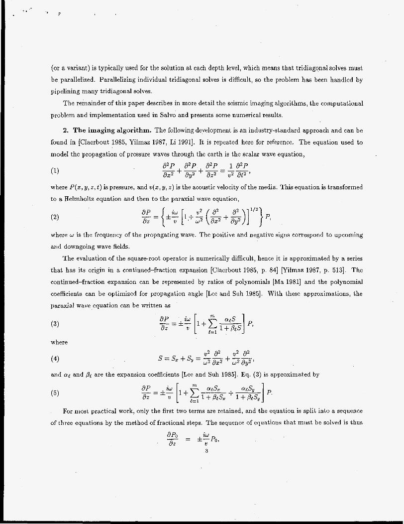
2. The imaging algorithm. The following development is an industry-standard approach and can be

found in [Claerbout 1985, Yilmaz 1987, Li 19911. It is repeated here for reference. The equation used to

model the propagation of pressure waves through the earth is the scalar wave equation,

d2P d2P d2P 1 d2P 8x2 ay2 8x2 v2 at2 ' -+- +---- -

where P(z, y, z , t) is pressure, and v(x, y, z ) is the acoustic velocity of the media. This equation is transformed

to a Helmholtz equation and then to the paraxial wave equation,

(1)

where w is the frequency of the propagating wave. The positive and negative signs correspond to upcoming

and downgoing wave fields.

The evaluation of the square-root operator is numerically difficult, hence it is approximated by a series

that has its origin in a continued-fraction expansion [Claerbout 1985, p. 841 [Yilmaz 1987, p. 5131. The

continued-fraction expansion can be represented by ratios of polynomials [Ma 19811 and the polynomial

coefficients can be optimized for propagation angle [Lee and Suh 19851. With these approximations, the

paraxial wave equation can be written as

(3)

where

(4) v2 8 2 v2 a 2 s=s,+s ---+--

w2 dy2 ' - w2 ax2

and a! and ,Be are the expansion coefficients [Lee and Suh 19851. Eq. (3) is approximated by

(5)

For most practical work, only the first two terms are retained, and the equation is split into a sequence

of three equations by the method of fractional steps. The sequence of equations that must be solved is thus

i W dPo 82 V

= &-Po, -

3

To obtain an image that is reasonably accurate for wave propagating at angles up to 6 5 O , we use a1 = 0.478242

and / 3 ~ = 0.376370. Other approximations are obtained by choosing different values for a and /3 and/or by

retaining more terms in (3) pilmaz 19871.

There are many sources of error introduced by solving the sequence of equations (6) instead of Eq. (2).

Several filters have been introduced to correct the errors (or a subset of the errors). One of these was

introduced in [Li 19911, in an attempt to correct all the errors after a transformation into Fourier space. The

primary computational operation in the Li filter is the FFT and the correction involves assumptions about

boundary conditions and the velocity model. Another filter was introduced in [Graves and Clayton 19901

in an aktempt to correct the error introduced by the approximations used to derive Eq. (5). The primary

computational operation in this filter is the solution of a tridiagonal linear system.

Tbe boundary conditions must be chosen so that no waves are reflected back into the domain. Several

possible absorbing boundary conditions are given in [Clayton and Engquist 19801. The best of these is the

boundary condition

(7)

where

a = l

b = { 1, left boundaries

e = { 2 - 2/&, left boundaries

- 1, right boundaries

2/& - 2, right boundaries

In phase-space, this is a hyperbola fit to the circle of the wave equation. The use of first order differences

in the boundary conditions maintains the tridiagonal structure of the resulting linear system. Salvo also

includes absorbing boundary conditions based on a Pad6 approximation [Xu 19961.

3. The computational problem. A seismic image can be computed using the equations above by

the following high-level algorithm.

4

Begin migration

Read source and receiver traces measured on the surface

Transform traces to frequency domain using an FFT

For each depth level

Read velocity

For each frequency being migrated

Migrate source and receiver traces one depth level

End for

Combine source and receiver data to create an image

Write image

End for

End migration

The computational “problem” to a large extent is based on the volume of data to be processed, Le., the

size of the problem. A typical marine seismic survey consists of between 10,000 and 100,000 shots. For each

shot, there are between 1500 and 3500 receiver traces, and receiver traces typically contain 2500 samples.

Thus, the input dataset can contain over 10 megabytes of data for each shot and over 1 terabyte bytes)

of data for the whole survey. The specific numbers for land surveys are different, but the survey dataset can

still be very large.

A typical processing grid for finite-difference, prestack migration is 500 x 200 x 1000 points, and up

to 1000 frequencies are migrated for both shot and receiver fields for a total of 2 x 10” grid points in the

(z, y, z , u ) comutational domain.

It is clear that a lot of data must be read, processed and written. In the following sections, we examine

issues related to 1/0 and processing speed. The discussion below is based on our implementation of finite-

difference, prestack, depth migration in a code called Salvo.

4. I/O. 1/0 is a large part of seismic imaging and some effort must be made to do it efficiently. There

are two parts to the 1/0 problem in finite-difference migration, the initial input in which data is read and

transformed to the frequency domain for processing, and the read (velocity)-write (image) pair that occurs

at every depth step. (Additional 1/0 is required if the computations do not fit in the computers main

memory, but we do not examine that issue here.) We describe our approach to both parts below, but there

are several general principles that should be adhered to in all cases.

The amount of 1/0 should be minimized. 5

0 interprocessor communication resulting from 1/0 should be minimized.

0 The 1/0 bandwidth should be maximized.

0 1/0 and computation should be overlapped.

The time required to read the initial seismic data, read the velocity models and write the images can be

substantial. In Salvo, the effect of the “I/O bottleneck” is mitigated by performing preliminary computations

and data redistribution using nodes not directly involved in the I/O.

The trace dataset is distributed across many disks to increase the total disk-to-memory bandwidth. A subset of the available nodes is assigned to handle the I/O. Each of these 1/0 nodes is assigned to handle

1/0 firom one file system.

The remaining nodes, termed compute nodes, can complete computations and communications nec-

essary before the migration can begin. Each compute node is assigned an 1/0 node, and performs the

pre-computations on the data read by its 1/0 node. Currently the pre-computation comprises fast Fourier

transfbrms (FFTs), but other computations could also be performed. If we assign a sufficient number of

compute nodes to each 1/0 node, the time to read a block of seismic data will be greater than the time

required to compute the FFTs and distribute the frequencies to the correct nodes for later computations.

Thus, the computation time will be hidden behind the 1/0 time.

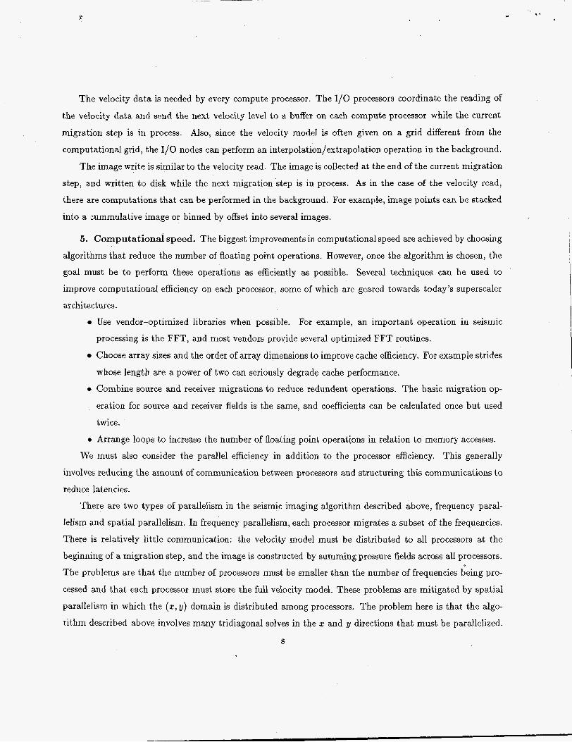
A model of the 1/0 and pre-computations and communications can be developed to determine the proper

balance between 1/0 nodes and compute nodes. The 1/0 node begins by reading a block of data from a disk

and distributing this data to a set of compute nodes. The time required for this operation is approximately

where (P is the disk bandwidth, b is the blocksize, a is communication latency, ,B is the time to communicate

one byCe, and c is the number of compute nodes.

After completing an FFT, the compute node must distribute each frequency to the processor assigned

to perform the seismic migration for that x and y location and frequency. The time to evenly distribute the

frequencies of one trace is approximated by

Pw [ a + P (31 i where p,,, is the number of nodes at a specific x and y location, that is, the number of nodes in the frequency

decomposition, n is the number of words in a frequency trace, g is the size of one word of data (g = 8 for

single precision, complex numbers). The total time required to FFT the traces and redistribute frequencies

6

a 50

P) 45-

z ' 40- Copt -

- 0 10 20 30 40 5 0 6 0 7 0

Frequency Nodes (Pw)

FIG. 1. The graph shows Copt as a function o f p w . Circles correspond t o actual runs in which 1/0 nodes had no idle time;

squares correspond t o actual Tuns in which I /O node weTe idle f o r part of the run.

for b / ( c n g ) traces, ( L e . , the number of traces which one compute node processes) is approximately

where T is the time to compute an FFT. T is machine and library dependent, and because T can be measured

easily on most platforms, it is not further decomposed into computational rates.

To determine the minimum number of compute nodes for each 1/0 node, C o p t , the time required to read

and distribute a block of data must be equal to or greater than the time required to FFT the time traces

and redistribute frequencies. This yields

-6 (a + P) + + (8) , Copt = 2cY

where

All of the variables in the expression for copt, except p,, are either machine constants or defined by the

problem size. Figure 1 shows the C o p t as a function of p , and points indicating several "real" runs. We

see that the model does a good job of predicting whether the run time is dominated by disk reads or by

computation and com'munication.

An 1/0 partition is also maintained during the computational phase to handle reading the velocity data

and writing the image data. Here, the computations are expected to be the bottleneck, and 1/0 is expected

to occur in the background; however, the basic principle of the 1/0 partition remains the same. 7

The velocity data is needed by every compute processor. The I/O processors coordinate the reading of

the velocity data and send the next velocity level to a buffer on each compute processor while the current

migrat,ion step is in process. Also, since the velocity model is often given on a grid different from the

computational grid, the 1/0 nodes can perform an interpolation/extrapolation operation in the background.

The image write is similar to the velocity read. The image is collected at the end of the current migration

step, and written to disk while the next migration step is in process. As in the case of the velocity read,

there axe computations that can be performed in the background. For example, image points can be stacked

into a cummulative image or binned by offset into several images.

5. Computational speed. The biggest improvements in computational speed are achieved by choosing

algorithms that reduce the number of floating point operations. However, once the algorithm is chosen, the

goal must be to perform these operations as efficiently as possible. Several techniques can be used to

improve computational efficiency on each processor, some of which are geared towards today’s superscaler

architectures.

Use vendor-optimized libraries when possible. For example, an important operation in seismic

processing is the FFT, and most vendors provide several optimized FFT routines.

Choose array sizes and the order of array dimensions to improve cache efficiency. For example strides

whose length are a power of two can seriously degrade cache performance.

0 Combine source and receiver migrations to reduce redundent operations. The basic migration op-

eration for source and receiver fields is the same, and coefficients can be calculated once but used

twice.

0 Arrange loops to increase the number of floating point operations in relation to memory accesses.

We must also consider the parallel efficiency in addition to the processor efficiency. This generally

involves reducing the amount of communication between processors and structuring this communications to

reduce latencies.

There are two types of parallelism in the seismic imaging algorithm described above, frequency paral-

lelism and spatial parallelism. In frequency parallelism, each processor migrates a subset of the frequencies.

There is relatively little communication: the velocity model must be distributed to all processors at the

beginning of a migration step, and the image is constructed by summing pressure fields across all processors.

The problems are that the number of processors must be smaller than the number of frequencies being pro-

cessed and that each processor must store the full velocity model. These problems are mitigated by spatial

parallelism in which the (c, y) domain is distributed among processors. The problem here is that the algo-

rithm described above involves many tridiagonal solves in the c and y directions that must be parallelized.

8

i ..

We have taken advantage of both types of parallelism, and our solution to the problem of tridiagonal solves

is described below.

It is difficult to parallelize the solution of a single tridiagonal system, but this difficulty is offset because

there are many such systems. Salvo takes advantage of this by setting up a pipeline. That is, in the first

stage of the pipeline, processor one starts a tridiagonal solve. In the second stage of the pipeline, processor

two continues the first tridiagonal solve, while processor one starts a second tridiagonal solve. This process

continues until all processors are busy.

In the implementation of a pipeline, there are two sources of parallel inefficiency. The first is communi-

cation between processors. This communication time is dominated by the message latency since very small

amounts of data must be transferred. This can be offset by grouping several tridiagonal solves into each

stage of the pipeline.

The second source of parallel inefficiency is processor idle time associated with the pipeline being filled

or emptied. This is dominated by the computation time of each pipeline stage. It can be reduced by reducing

the computation time, but it is increased by grouping several tridiagonal solves in each stage of the pipeline.

The total parallel overhead can be minimized by choosing the number of tridiagonal solves that are

grouped into each stage of the pipeline. The optimal number of tridiagonal solves to group is based on the

following model. The communication time is approximated by

Q Tcomm = N (26 -t 24P) ,

where N is the total number of tridiagonal solves, b is the number to be grouped into each stage of the

pipeline, a is the communication latency, and ,B is time to communicate one byte. The pipeline idle time is

approximated by

where W is the total number of floating point operations required at each grid point, n is the number of

points in each stage of the pipeline, p is the number of processors in the pipeline, and y is the computational

time required for one floating point operation.

The value of b that minimizes the total overhead, bmin is computed by summing T,,,, and Tpipe, and

minimizing. This yields

W n 2 N a y + 2 4 p P Yi2 bmin = ( We have found this model to be quite accurate, and all results presented later in this paper use this

value of bmin. 9

6. Results. To validate Salvo, several tests were performed to ensure accurate imaging of reflecting

layers. The problems selected for the test cases include a simple impulse response from a hemispherical

reflector, the ARCO-French Model [French 19741, the Marmousi model, the SEG/EAEG 3D overthrust

model [Aminzadeh e t ai. 19941, the SEG/EAEG 3D salt model, and real data.

As an example of a Salvo migration, we show the 3D SEG/EAEG salt model. This is a synthetic

model with synthetic receiver data available through the SEG internet home page at http://www.seg.com.

Figure 2(a) shows a corner-cut view of the model. The grayscale colormap indicates the speed of sound in

a region; the lighter a region, the higher the speed. The white region is the salt dome. Figure 2(b) shows

the same corner-cut view of the image produced by Salvo. The image is 600 x 600 x 210. It is a stack of 45 shots, each processed on a 200 x 200 x 210 grid with a surface grid fully populated with receivers. For this

image AZ = Ay = Az = 20 meters. The receiver traces contain 626 samples with At = 0.004 seconds, and

511 frequencies were migrated. Some additional postprocessing of the images has been performed by ARC0

and Oryx Energy Company.

To test the computational performance of Salvo, the sample impulse problem was run on the Intel

Paragon. The spatial size of the impulse problem has been adjusted so that each processor has approximately

a 101 x 101 spatial grid. Sixty-four frequencies have been retained for the solution independent of how many

frequency processors were used.

Timings for the sample impulse run are shown in Table 1. From these numbers, we can make a few

statements about the parallelism of the migration routine. First, the spatial parallelism is very efficient

as soon as the pipeline is fully utilized (after 3 x 3 x 1 processor mesh). However there is a penalty for

introducing the pipeline in each direction, which is about 10% for each (Le . , 1 x 1 x 1 at 100% to 91% for

2 x 1 x 1, and to 81% for 2 x 2 x 1). The origins of this “overhead” is still under investigation.

Second, the frequency parallelism is very efficient, staying in the upper 90’s for most of the problems.

This is expected, since frequency parallelism requires little communication during the solve. The primary

communications are a broadcast of velocity data at the beginning of each depth step and a summation to

produce an image at the end of each depth step.

For an additional timing figure, we ran a 2000 x 2000 x 1000 impulse problem with 140 frequencies on a

1,792-node Intel Paragon. Each node processed a 250 x 250, 2-y subdomain with 5 frequencies. The total

run time was 7 hrs., 51 mins, which corresponds to a computational rate of 22 Mflops/second/node.

7. Conclusions. In this paper, an implementation of a wave-equation-based, finite-difference, prestack,

depth migration code for MPP computers has been presented. The results of several test runs were presented

to show the accuracy of the code. Also, timing results and performance models have been presented to show

10

(b)

FIG. 2. A corner-cut view of the SEG/EAEG 30 salt model and ihe same corner cut view of the Salvo image produced

b y processing 45 shots.

that the code can be tuned to run efficiently on MPP computers.

[Aminzadeh et al. 19941

[ B u n k s 19951

[Claerbout 19851

REFERENCES

Aminzadeh, F.; N. Burkhard; L. Nicoletis; F. Rocca; K. Wyatt. 1994. “SEG/EAEG 3-D Modeling Project: 2nd Update.” Leading Edge. September, 949-952.

Bunks, C. 1995. “Effective Filtering of Artifacts for Implicit Finite-Difference Paraxial Wave

Equation Migration.” Geophysical Prospecting, vol. 43: 203-220.

Claerbout, J. F. 1985. Imaging the Earth’s Interior. Blackwell Scientific Publications,

Boston.

11

. ...

I p , x p , x pw I Runtime (sec.) Efficiency (%) I l x l x l

2 x l x 1

2 X 2 X 1

3 x 3 ~ 1

4 x 4 ~ 1

5 x 5 ~ 1

6 x 6 ~ 1

7 x 7 ~ 1

8 x 8 ~ 1

Spatial Parallelism

84.1

92.4

103.2

108.7

108.9

112.2

114.8

115.6

116.2

100.0

91.0

81.5

77.4

77.2

75.0

73.3

72.8

72.4

l x l x l

1 x l x 2

1 x 1 ~ 4

1 x 1 ~ 8

1 x 1 ~ 1 6

1 x 1 ~ 3 2

1 x 1 ~ 6 4

Frequency Parallelism

84.1 100.0

42.21 99.6

21.19 99.2

10.63 98.9

5.35 98.2

2.71 97.0

1.40 93.8 TABLE 1

Timings f o r a sample impulse problem f o r spatial, frequency, and mixed parallelism on the Intel Paragon. Single processor times an: estimated. All other times are measured.

[Clayton and Engquist 19801

[Fletcher 19881

French 1974]

[Graves and Clayton 19901

[Lee and S m h 19851

Clayton, R. and B. Engquist. 1980 “Absorbing Boundary Conditions for Wave-Equation

Migration,” Geophysics, vol. 45, 895-904.

Fletcher, C. 1988 Computational Techniques for Fluid Dynamics Vol. I. Springer-Verlag,

Berlin.

French, W. S. 1974. “Two-Dimensional and Three-Dimensional Migration of Model-

Experiment Reflection Profiles.” Geophysics, vol. 39, 265-277.

Graves, R. and R. Clayton. 1990. “Modeling Acoustic Waves with Paraxial Extrapolators.”

Geophysics, vol. 55,306-319.

Lee, M. W. and S. Y . Suh. 1985. “Optimization of One-way Wave Equations.” Geophysics, VOI. 50, 1634-1637.

Li, Z. 1991. “Compensating Finite-Difference Errors in 3-D Migration and Modeling.” Geo- physics, V O ~ . 56, 1650-1660.

12

Ma, Z. 1981 “Finite-Difference Migration with Higher Order Approximation.” In 1981 Joint

Mtg. Chinese Geophys. Soc. a n d Society of Exploration Geophysicists, Society of Ex-

ploration Geophysicists.

xu, L. 1996 Working Notes on Absorbing Bozlndary Conditions f o r Prestack Depth Migra-

tion.

Yilmaz, 0. 1987. Seismic Data Processing, Investigations in Geophysics No. 2. P.O. Box

702740, Tulsa, OK 74170-2740: Society of Exploration Geophysicists.

[Ma 19811

[Xu 19961

pilmaz 19871

13