3d mhd coronal oscillations about a magnetic null … charpit’s method and a runge-kutta numerical...

arX

iv:0

712.

1731

v1 [

astr

o-ph

] 1

1 D

ec 2

007

Solar PhysicsDOI: 10.1007/•••••-•••-•••-••••-•

3D MHD Coronal Oscillations About a Magnetic

Null Point: Application of WKB Theory

J.A. McLaughlin · J.S.L. Ferguson · A.W.Hood

Received 27 September 2007; accepted 4 December 2007

c© Springer ••••

Abstract This paper is a demonstration of how the WKB approximation can beused to help solve the linearised 3D MHD equations. Using Charpit’s Method and aRunge-Kutta numerical scheme, we have demonstrated this technique for a potential3D magnetic null point, B = (x, ǫy − (ǫ+ 1) z). Under our cold plasma assumption,we have considered two types of wave propagation: fast magnetoacoustic and Alfvénwaves. We find that the fast magnetoacoustic wave experiences refraction towards themagnetic null point, and that the effect of this refraction depends upon the Alfvénspeed profile. The wave, and thus the wave energy, accumulates at the null point.We have found that current build up is exponential and the exponent is dependentupon ǫ. Thus, for the fast wave there is preferential heating at the null point. Forthe Alfvén wave, we find that the wave propagates along the fieldlines. For an Alfvénwave generated along the fan-plane, the wave accumulates along the spine. For anAlfvén wave generated across the spine, the value of ǫ determines where the waveaccumulation will occur: fan-plane (ǫ = 1), along the x−axis (0 < ǫ < 1) or alongthe y−axis (ǫ > 1). We have shown analytically that currents build up exponentially,leading to preferential heating in these areas. The work described here highlights theimportance of understanding the magnetic topology of the coronal magnetic field forthe location of wave heating.

Keywords: Magnetohydrodynamics; Waves, Propagation; Magnetic fields, Models;Heating, Coronal

1. Introduction

The WKB approximation is an asymptotic approximation technique which can beused when a system contains a large parameter (see e.g. Bender and Orszag, 1978).Hence, the WKB method can be used in a system where a wave propagates through abackground medium which varies on some spatial scale which is much longer than thewavelength of the wave. The SOHO and TRACE satellites have recently observedMHD wave motions in the corona, i.e. fast and slow magnetoacoustic waves and

School of Mathematics and Statistics, University of StAndrews, St Andrews, Fife, KY16 9SS, UK email:[email protected]

http://arxiv.org/abs/0712.1731v1

J.A. McLaughlin et al.

Alfvén waves (see reviews by Nakariakov and Verwichte, 2005; De Moortel, 2005;2006). The coronal magnetic field plays a fundamental role in their propagation andto begin to understand this inhomogeneous magnetised environment, it is useful tolook at the structure (topology) of the magnetic field itself. Potential-field extrapo-lations of the coronal magnetic field can be made from photospheric magnetograms.Such extrapolations show the existence of an important feature of the topology: null

points. Null points are points in the field where the magnetic field, and hence theAlfvén speed, is zero. Detailed investigations of the coronal magnetic field, using suchpotential field calculations, can be found in Beveridge, Priest, and Brown (2002) andBrown and Priest (2001).

McLaughlin and Hood (2004) found that for a single 2D null point, the fastmagnetoacoustic wave was attracted to the null and the wave energy accumulatedthere. In addition, they found that the Alfvén wave energy accumulated along theseparatrices of the topology. They solved the 2D linearised MHD equations numer-ically and compared the results with a WKB approximation: the agreement wasexcellent. From their work and other examples (e.g. Galsgaard, Priest, and Titov,2003; McLaughlin and Hood, 2005; 2006a; Khomenko and Collados, 2006) it hasbeen clearly demonstrated that the WKB approximation can provide a vital linkbetween analytical and numerical work, and often provides the critical insight tounderstanding the physical results. This paper demonstrates the methodology ofhow to apply the WKB approximation in linear 3D MHD. We believe that withthe vast amount of 3D modelling currently being undertaken, applying this WKBtechnique to 3D will be very useful and beneficial to modellers in the near future.

The work undertaken by Galsgaard, Priest, and Titov (2003) deserves specialmention here. They performed numerical experiments on the effect of twisting thespine of a 3D null point, and described the resultant wave propagation towardsthe null. They found that when the fieldlines around the spine are perturbed in arotationally symmetric manner, a twist wave (essentially an Alfvén wave) propagatestowards the null along the fieldlines. Whilst this Alfvén wave spreads out as the nullis approached, a fast-mode wave focuses on the null and wraps around it. Theyconcluded that the driving of the fast wave was likely to come from a non-linearcoupling to the Alfvén wave (Nakariakov, Roberts, and Murawski, 1997). They alsocompare their results with a WKB approximation and find that, for the β = 0 fastwave, the wavefront wraps around the null point as it contracts towards it. Theyperform their WKB approximation in cylindrical polar coordinates and thus theirresultant equations are two-dimensional (since a simple 3D null point is essentially2D in cylindrical coordinates). In contrast, we solve the WKB equations for threeCartesian components, and thus we can solve for more general disturbances and moregeneral boundary conditions. This also allows us to concentrate on the transientfeatures that are not always apparent when only cylindrically symmetric solutionsare permitted.

More recently, Pontin and Galsgaard (2007) and Pontin, Bhattacharjee, and Gals-gaard (2007) have performed numerical simulations in which the spine and fan ofa 3D null point are subject to rotational and shear perturbations. They found thatrotations of the fan plane lead to current sheets in the location of the spine androtations about the spine lead to current sheets in the fan. In addition, shearingperturbations lead to 3D localised current sheets focused at the null point itself.This general behaviour is in good agreement with the work presented in this paper,

McLaughlin3DWKB.tex; 29/05/2018; 3:13; p.2

Application of WKB Theory to 3D MHD

i.e. current accumulation at certain parts of the topology. However, the primary mo-tivation in Pontin and Galsgaard (2007) and Pontin, Bhattacharjee, and Galsgaard(2007) was to investigate current-sheet formation and reconnection rates, whereasthe techniques described in this paper focus on MHD wave-mode propagation andinterpretation.

The propagation of fast magnetoacoustic waves in an inhomogeneous coronalplasma has been investigated by Nakariakov and Roberts (1995), who showed howthe waves are refracted into regions of low Alfvén speed. In the case of null points,the Alfvén speed actually drops to zero.

The paper has the following outline: In Section 2, the basic equations are de-scribed. Section 3 details the 3D WKB approximation utilised in this paper. Theresults for the fast wave and Alfvén waves are shown in Section 4 and 5. Theconclusions and discussion are presented in Section 7. There are four appendiceswhich complement the results in the main text.

2. Basic Equations

The usual resistive, adiabatic MHD equations for a plasma in the solar corona areused:

ρ∂v

∂t+ ρ (v · ∇)v = −∇p+ j×B+ ρg , (1)

∂B

∂t= ∇× (v×B) + η∇2

B , (2)

∂ρ

∂t+∇ · (ρv) = 0 , (3)

∂p

∂t+ v · ∇p = −γp∇.v , (4)

µ j = ∇×B , (5)

where v is the plasma velocity, ρ is the mass density, p is the gas pressure, B isthe magnetic induction (usually called the magnetic field), j is the electric current,g is gravitational acceleration, γ is the ratio of specified heats, η is the magneticdiffusivity and µ is the magnetic permeability.

2.1. Basic Equilibrium

We choose a 3D magnetic null point for our equilibrium field, of the form:

B0 =B

L(x, ǫy,− (ǫ+ 1) z) , (6)

where B is a characteristic field strength, L is the length scale for magnetic fieldvariations and the parameter ǫ is related to the predominate direction of alignmentof the fieldlines in the fan plane. Parnell et al. (1996) investigated and classified thedifferent types of linear magnetic null points that can exist (our ǫ parameter is calledp in their work). Topologically, this 3D null consists of two key parts: the z−axisrepresents a special, isolated fieldline called the spine which approaches the null fromabove and below (Priest and Titov, 1996) and the xy−plane through z = 0 is known



Figure 1. Left : Proper radial null point, described by B = (x, y,−2z), i.e. ǫ = 1. Right :Improper radial null point, described by B = (x, 1

2y,− 3

2z), i.e. ǫ = 1

2. Note for ǫ = 1

2, the

field lines rapidly curve such that they run parallel to the x−axis along y = 0. In both figures,the z−axis indicates the spine and the xy−plane at z = 0 denotes the fan. The red fieldlineshave been tracked from the z = 1 plane, the blue from z = −1.

as the fan and consists of a surface of fieldlines spreading out radially from the null.Figure 1 shows two examples of 3D null points: ǫ = 1 (left) and ǫ = 1/2 (right).Titov and Hornig (2000) have investigated the steady state structures of magneticnull points.

Equation (6) is the general expression for the linear field about a potential mag-netic null point (Parnell et al., 1996: Section IV). In this paper, we only considerǫ ≥ 0 and so all nulls we describe are positive nulls, i.e. the spine points into the nulland the field lines in the fan are directed away. In addition, all potential nulls aredesignated radial, i.e. there is no spiral motions in the fan-plane. In general, thereare three cases to consider:

• ǫ = 1: describes a proper null (Figure 1: Left). This magnetic null has cylindricalsymmetry about the spine axis.

• ǫ > 0, ǫ 6= 1: describes an improper null (Figure 1: Right). Field lines rapidlycurve such that they run parallel to the x−axis if 0 < ǫ < 1 and parallel to they−axis if ǫ > 1.

• ǫ = 0: equation (6) reduces to the X-point potential field in the xz−plane andforms a null line along the y−axis through x = z = 0. MHD wave propagationin this 2D configuration has been studied extensively by McLaughlin and Hood(2004; 2005; 2006a).

2.2. Assumptions and Simplifications

In this paper, the linearised MHD equations are used to study the nature of wavepropagation near the null point. Using subscripts of 0 for equilibrium quantities and1 for perturbed quantities, Equations (1) – (5) become:

ρ0∂v1

∂t= −∇p1 + j0 ×B1 + j1 ×B0 + ρ1g , (7)



∂B1

∂t= ∇× (v1 ×B0) + η∇2

B1 , (8)

∂ρ1∂t

+ ∇ · (ρ0v1) = 0 , (9)

∂p1∂t

+ v1.∇p0 = −γp0∇ · v1 , (10)

µ j1 = ∇×B1 . (11)

We now consider several simplifications to our system. We will only be consideringa potential equilibrium magnetic field (∇×B0 = 0) in an ideal system (η = 0). Wewill also assume the equilibrium gas density (ρ0) is uniform. A spatial variation in ρ0can cause phase mixing (Heyvaerts and Priest, 1983; De Moortel et al., 1999; Hood,Brooks, and Wright, 2002). In addition, we ignore the effect of gravity on the system(i.e. we set g = 0). Finally, in this paper we assume a cold plasma, i.e. cs =√

γp0/ρ0 = 0.We will not discuss Equation (9) further as it can be solved once we know v1. In

fact, under the assumptions of linearisation and no gravity, it has no influence on themomentum equation and so in effect the plasma is arbitrarily compressible (Craigand Watson, 1992).

We now non-dimensionalise the above equations as follows: let v1 = v̄v∗1 , B0 =

BB∗0, B1 = BB∗

1, x = Lx∗, z = Lz∗, ∇ = 1L∇

∗ and t = t̄t∗, where we let ∗ denotea dimensionless quantity and v̄, B, L, and t̄ are constants with the dimensions ofthe variable that they are scaling. In addition, ρ0 and p0 are constants as theseequilibrium quantities are uniform (i.e. ρ∗0 = p∗0 = 1). We then set B/

√µρ0 = v̄ and

v̄ = L/t̄ (setting v̄ as a constant background Alfvén speed). Under these scalings,t∗ = 1 (for example) refers to t = t̄ = L/v̄; i.e. the (background) Alfvén time takento travel a distance L. For the rest of this paper, we drop the star indices; the factthat they are now non-dimensionalised is understood.

These non-dimensionalised equations can be combined to form one single equa-tion:

∂2

∂t2v1 = {∇ × [∇× (v1 ×B0)]} ×B0 . (12)

3. WKB Approximation

In this paper, we will be looking for WKB solutions of the form:

v = aeiφ(x,y,z,t) (13)

where a is a constant. In addition, we define ω = φt as the frequency and k = ∇φ =(φx, φy , φz) = (p, q, r) as the wavevector. φ, and its derivatives, are considered to bethe large parameters in our system.

One of the difficulties associated with 3D MHD wave propagation is distinguishingbetween the three different wave types, i.e. between the fast and slow magnetoacous-tic waves and the Alfvén wave. To aid us in our interpretation, we now define a newcoordinate system: (B0,k,B0×k), where k is our wavevector as defined above. Thiscoordinate system fully describes all three directions in space when B0 and k are notparallel to each other, i.e. k 6= λB0, where λ is some constant of proportionality. In



the work below, we will proceed assuming k 6= λB0. The scenario where k = λB0 islooked at in Appendix A. In fact, the work described below is also valid for k = λB0

with the consequence that the solution is degenerate, i.e. the waves recovered areidentical and cannot be distinguished.

We now substitute v = aeiφ(x,y,z,t) into Equation (12) and make the WKBapproximation such that φ ≫ 1. Taking the dot product with B0, k and B0 × k

gives three velocity components which, in matrix form, are:

ω2 0 0

(B0 · k) |k|2 ω2 − |B0|2 |k|2 0

0 0 ω2 − (B0 · k)2

v ·B0

v · kv ·B0 × k

=

000

The matrix of these three coupled Equations must have zero determinant so as notto have a trivial solution. Thus, taking the determinant gives:

F (φ, ω, t,B0,k) =(

ω2 − 0)(

ω2 − |B0|2 |k|2)(

ω2 − (B0 · k)2)

= 0 , (14)

where F is a first-order, non-linear PDE. Equation (14) has two solutions, corre-sponding to two different MHD wave types (in general three, but the slow wave hasvanished under the cold plasma approximation). The two solutions correspond tothe fast magnetoacoustic wave and to the Alfvén wave.

In Sections 4 and 5, we will examine each of these wave solutions in detail for the3D magnetic null point configuration described by Equation (6) for both ǫ = 1/2and ǫ = 1. However, it should be noted that the technique described above is validfor any 3D magnetic configuration. The case where the two roots of Equation (14)are the same is examined in Appendix A.

4. Fast Wave

Let us first consider the fast wave solution, and hence we assume ω2 6= (B0 · k)2.Thus, Equation (14) simplifies to:

F (φ, ω, t,B0,k) = ω2 − |B0|2 |k|2

= ω2 −(

x2 + ǫ2y2 + (ǫ+ 1)2 z2)(

p2 + q2 + r2)

= 0 (15)

We can now use Charpit’s Method (see e.g. Evans, Blackledge, and Yardley, 1999) tosolve this first-order PDE, where we assume our variables depend upon some inde-pendent parameter s in characteristic space. Charpit’s Method replaces a first-orderPDE with a set of characteristics that are a system of ODEs. Charpit’s Equationstake the form:

dφ

ds=

(

ω∂

∂ω+ k · ∂

∂k

)

F ,dt

ds=

∂

∂ωF ,

dx

ds=

∂

∂kF ,

dω

ds= −

(

∂

∂t+ ω

∂

∂φ

)

F ,dk

ds= −

(

∂

∂x+ k

∂

∂φ

)

F ,

where, as previously defined, k = (p, q, r) and x = (x, y, z). In general, the coupledEquations have to be solved numerically, but analytical solutions have been found in



2D (McLaughlin and Hood, 2004). These ODEs are subject to the initial conditionsφ = φ0(s = 0), x = x0(s = 0), y = y0(s = 0), z = z0(s = 0), t = t0(s = 0),p = p0(s = 0), q = q0(s = 0), r = r0(s = 0), and ω = ω0(s = 0) and, in thefollowing work, are solved numerically using a fourth-order Runge-Kutta method.

In addition, note that there are no boundary conditions in the usual sense: thevariables are solved using Charpit’s Method (essentially the method of character-istics) and the resulting characteristics are only dependent upon initial position(x0, y0, z0, t0) and distance travelled along the characteristic; s. Thus, there areno computational boundaries and no boundary conditions (only initial conditions).In this paper, we have chosen to illustrate our results in the domain −1 ≤ x ≤ 1,−1 ≤ y ≤ 1, −1 ≤ z ≤ 1, and this choice is arbitrary. That the WKB solutionsare independent of boundary conditions is actually an advantage over traditionalnumerical simulations; where the choice of boundary conditions can play a significantrole.

For the fast wave (Equation 15) Charpit’s Equations are:

dφ

ds= 0 ,

dt

ds= ω ,

dx

ds= −pA ,

dy

ds= −qA ,

dz

ds= −rA

dω

ds= 0 ,

dp

ds= xB ,

dq

ds= ǫ2yB ,

dr

ds= (ǫ+ 1)2 zB (16)

where A = x2 + ǫ2y2 + (ǫ+ 1)2 z2 and B = p2 + q2 + r2.From these Equations, we note that φ = constant = φ0 and ω = constant = ω0,

i.e. constant frequency. In addition, t = ωs + t0, where we arbitrarily set t0 = 0,which correponds to the leading edge of the wave pulse starting at t = 0 when s = 0.We can also construct the integral:

d

ds(xp+ yq + zr) = 0 ⇒ xp+ yq + zr = constant = x0p0 + y0q0 + z0r0 (17)

However, we are unable to find a second conserved quantity.

4.1. Planar fast wave starting at z0 = 1

We now solve Equation (16) subject to the initial conditions:

φ0 = 0 , ω0 = 2π , −1 ≤ x0 ≤ 1 , −1 ≤ y0 ≤ 1 , z0 = 1 ,

p0 = 0 , q0 = 0 , r0 = ω0/

√

x20 + ǫ2y20 + (ǫ+ 1)2 z20 , (18)

where we have arbitrarily chosen ω0 = 2π and φ0 = 0. These initial conditionscorrespond to a planar fast wave being sent towards the null point from our upperboundary (along z = z0).

Let us initially consider ǫ = 1 (corresponding to Figure 1: Left). In Figure 2, wehave plotted surfaces of constant φ, which can be thought of as defining the positionof the wavefront, at various times. Since t = ωs, these correspond to different valuesof the parameter s, which quantifies distance travelled along the characteristic curve.We can clearly see that the fast wave experiences a refraction effect towards the nullpoint, i.e. propagation towards regions of lower Alfvén speed. A similar refraction



Figure 2. (ǫ = 1) Surfaces of constant φ at four values of t, showing the behaviour of the(initially planar) wavefront that starts at −1 ≤ x ≤ 1, −1 ≤ y < 0 and z = 1 (blue) and−1 ≤ x ≤ 1, 0 ≤ y ≤ 1 and z = 1 (red). The (arbitrary) colouring has been added to aid thereader in tracking the wave behaviour. This figure is also available as an mpg animation.

effect was also seen in the 2D case (McLaughlin and Hood, 2004; 2006a). Thus, thefast wave is deformed from its initial planar profile. The wave, and hence all thewave energy, eventually accumulate at the null point.

We can also use our WKB solution to plot the ray paths of individual fluidelements from the initial wave. In Figure 3, we can see the ray paths for fluid elementsthat begin at four different starting points in the z0 = 1 plane. These four ray pathsare typical of the behaviour of the fast wave fluid elements (more examples can beseen in the associated mpg movie). We can clearly see the refraction effect wrappingthe fast wave fluid elements around the null point.

Note that the magnitude of the refraction effect is the same for each fluid elementthat starts at the same radius from z = z0. Thus, the xy−plane projections arealways straight lines. This is because the Alfvén speed is the same for elementsstarting at the same radius from z = z0, i.e. vA(x0, y0, z0) =

√

x20 + y20 + 4z20 , andthe behaviour of the fast wave is entirely dominated by the Alfvén speed profile. Forǫ = 1, isosurfaces of Alfvén speed form prolate spheroids (parallel to the spine).

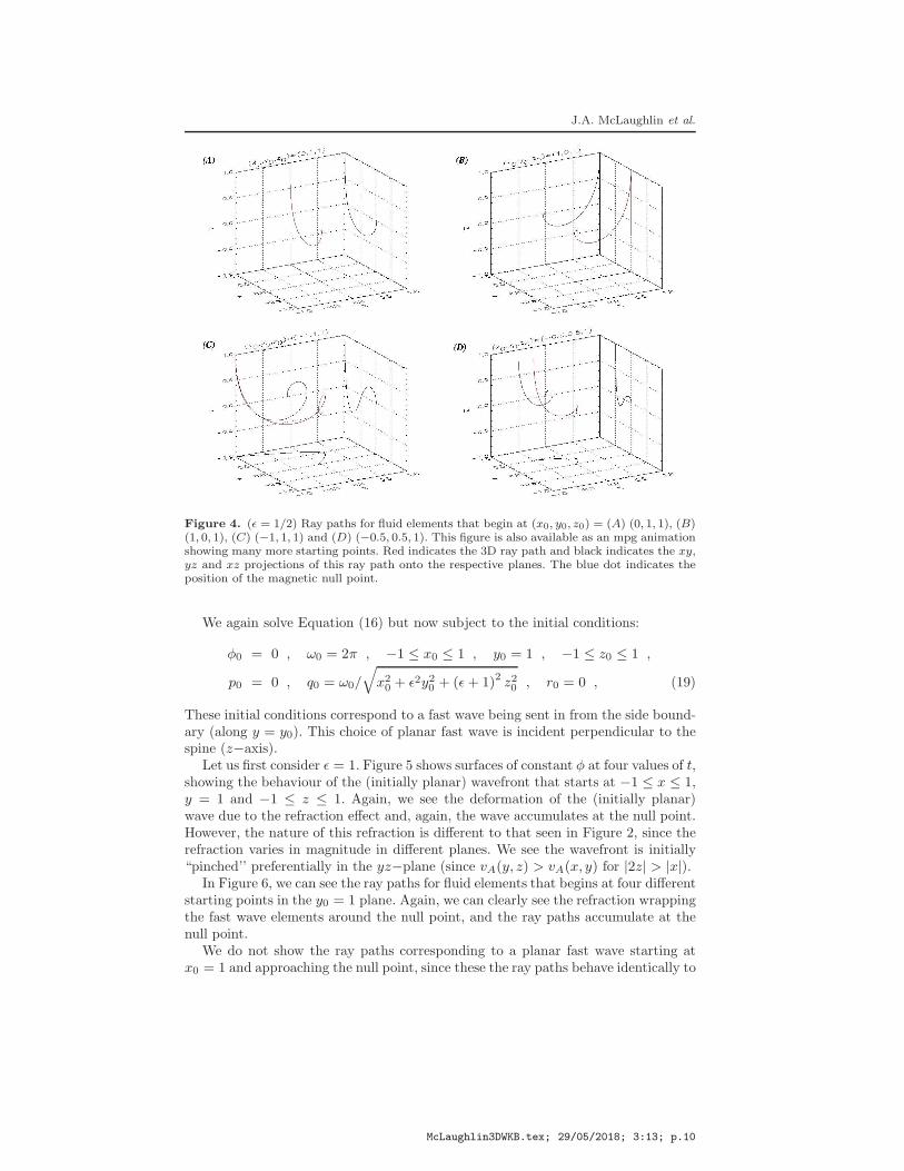
Let us now extend our study to improper null points. In Figure 4, we can seethe ray paths for fluid elements that begin at the same four starting points as inFigure 3, but now for the magnetic field configuration seen in Figure 1: Right, i.eǫ = 1/2. The first thing to note is that the refraction effect still occurs in thisconfiguration, as expected, and that the fluid elements still eventually accumulateat the null point. However, the individual ray paths are different to those for ǫ = 1.



Figure 3. (ǫ = 1) Ray paths for fluid elements that begin at (x0, y0, z0) = (A) (0, 1, 1), (B)(1, 0, 1), (C) (−1, 1, 1) and (D) (−0.5, 0.5, 1). This figure is also available as an mpg animationshowing all −1 ≤ x0 ≤ 1, z0 = 1 along y = −1 and y = 1, and all −1 ≤ y0 ≤ 1, z0 = 1 alongx = −1 and x = 1. Here, red indicates the 3D ray path and black indicates the xy, yz and xzprojections of this ray path onto the respective planes. The blue dot indicates the position ofthe magnetic null point.

Comparing panels 4A and 4B with 3A and 3B, we see that along x = 0 or y = 0,the ray paths are very similar. However, the distance travelled by the fluid elementis actually different in the ǫ = 1/2 simulation since the Alfvén speeds, and hencethe magnitude of the refraction, has changed. In fact, the refraction is weaker alongy = 0 (since for |B| = x2 + ǫ2y2 + (ǫ+ 1)2 z2, |B|ǫ=1 > |B|ǫ=1/2 along y = 0) andso the fluid element travels a longer distance than the equivalent ǫ = 1 fluid element.Along x = 0, the effect is more complicated, with |B|ǫ=1 > |B|ǫ=1/2 only true for

|z| > |y|.The differences in the ray paths are much more obvious when comparing panels

4C and 4D with 3C and 3D. For ǫ = 1/2, we see that the ray paths are now“corkscrew’’ spirals. This is because the Alfvén speed profile is now varying in threedirections, whereas for ǫ = 1 the Alfvén speed essentially varies in two directions:r =

√

x2 + y2 and z. Thus, the xy−plane projections are no longer straight lines.For ǫ = 1/2, isosurfaces of Alfvén speed form scalene ellipsoids.

4.2. Planar fast wave starting at y0 = 1



Figure 4. (ǫ = 1/2) Ray paths for fluid elements that begin at (x0, y0, z0) = (A) (0, 1, 1), (B)(1, 0, 1), (C) (−1, 1, 1) and (D) (−0.5, 0.5, 1). This figure is also available as an mpg animationshowing many more starting points. Red indicates the 3D ray path and black indicates the xy,yz and xz projections of this ray path onto the respective planes. The blue dot indicates theposition of the magnetic null point.

We again solve Equation (16) but now subject to the initial conditions:

φ0 = 0 , ω0 = 2π , −1 ≤ x0 ≤ 1 , y0 = 1 , −1 ≤ z0 ≤ 1 ,

p0 = 0 , q0 = ω0/

√

x20 + ǫ2y20 + (ǫ+ 1)2 z20 , r0 = 0 , (19)

These initial conditions correspond to a fast wave being sent in from the side bound-ary (along y = y0). This choice of planar fast wave is incident perpendicular to thespine (z−axis).

Let us first consider ǫ = 1. Figure 5 shows surfaces of constant φ at four values of t,showing the behaviour of the (initially planar) wavefront that starts at −1 ≤ x ≤ 1,y = 1 and −1 ≤ z ≤ 1. Again, we see the deformation of the (initially planar)wave due to the refraction effect and, again, the wave accumulates at the null point.However, the nature of this refraction is different to that seen in Figure 2, since therefraction varies in magnitude in different planes. We see the wavefront is initially“pinched’’ preferentially in the yz−plane (since vA(y, z) > vA(x, y) for |2z| > |x|).

In Figure 6, we can see the ray paths for fluid elements that begins at four differentstarting points in the y0 = 1 plane. Again, we can clearly see the refraction wrappingthe fast wave elements around the null point, and the ray paths accumulate at thenull point.

We do not show the ray paths corresponding to a planar fast wave starting atx0 = 1 and approaching the null point, since these the ray paths behave identically to



Figure 5. (ǫ = 1) Surfaces of constant φ at four values of t, showing the behaviour of the(initially planar) wavefront that starts at −1 ≤ x ≤ 1, y = 1 and −1 ≤ z < 0 (blue) and−1 ≤ x ≤ 1, y = 1 and 0 ≤ z ≤ 1 (red). The (arbitrary) colouring has been added to aid thereader in tracking the wave behaviour. The yellow dot indicates the position of the magneticnull point.

those in Figure 6 under the transformation (x, y) → (−y, x) (for ǫ = 1 configuration).The ray paths corresponding to a planar fast wave starting at y0 = 1 and startingat x0 = 1 in the ǫ = 1/2 magnetic configuration can be found in Figures 11 and 12in Appendix B.

Thus, Sections 4.1 and 4.2 have shown that the fast wave experiences a refractioneffect in the neighbourhood of a 3D magnetic null point and that in all of thesecases, the main result is the same: the ray paths accumulate at the null point. Ofcourse, the actual paths taken vary depending upon initial conditions and choice ofǫ. Hence, we conclude that the fast wave, and thus the fast-wave energy, eventuallyaccumulate at the 3D null point for all ǫ and all initial conditions that generate awave approaching the null.

Finally, it should be noted that the behaviour of the fast wave is entirely domi-nated by the Alfvén-speed profile, and since the magnetic field drops to zero at thenull point, the wave will never actually reach there. However, there is still currentaccumulation and hence non-ideal effects may be able to extract the wave energy ina finite time. This is investigated in the next section.

4.3. Current build up

From Section 3, we know that for the fast wave v · B0 = 0 and v · (B0 × k) = 0.This gives us two Equations for the three velocity variables:

xvx + ǫyvy − (ǫ+ 1) zvz = 0 ,

[ǫyr + (ǫ+ 1) zq] vx − [xr + (ǫ+ 1) zp] vy + [xq − ǫyp] vz = 0 .

Thus, we can express two of the velocity components in terms of the third.



Figure 6. (ǫ = 1) Ray paths for fluid elements that begin at (x0, y0, z0) = (A) (0, 1, 1), (B)(−1, 1, 0), (C) (−1, 1, 1) and (D) (−0.5, 1, 0.5). This figure is also available as an mpg animationshowing many more starting points. Red indicates the 3D ray path and black indicates the xy,yz and xz projections of this ray path onto the respective planes. The blue dot indicates theposition of the magnetic null point.

Recall from Section 2 that the perturbed electric current is given by j1 = ∇×B1.

Thus,

∂

∂tB1 = ∇× (v ×B0) ⇒ −ωB1 = k× (v×B0) ,

⇒ j1 = ik×B1 = −ik× [k× (v×B0)] /ω = i |k|2 (v×B0) /ω ,

where we have made use of v · (B0 × k) = 0. From Equation (15), we can substitute

for |k|2 to obtain:

j1 = iω (v ×B0) /|B0|2

= iω[− (ǫ+ 1) zvy − ǫyvz, (ǫ+ 1) zvx + xvz , ǫyvx − xvy]

x2 + ǫ2y2 + (ǫ+ 1)2 z2,

⇒ |j1| = ω |v| / |B0| , (20)

where we have used v ·B0 = 0 to simplify |v ×B0|. Thus, since |v| is bounded (from

our assumed form of v seen in Equation 13) we can see that the current associated

with the fast wave will grow ∼ 1/ |B0|. Equivalent behaviour was found for the fast

wave in the 2D case (McLaughlin and Hood, 2004), i.e. ǫ = 0.



Moreover, we can place limits on the magnitude of the current build up. FromEquation (37) in Appendix C, we can place limits on |j1| such that:

ω |v|(ǫ+ 1)R0

eαǫ2t/ω0 ≤ |j1| ≤

ω |v|ǫ R0

eα(ǫ+1)2t/ω0 , (21)

where R20 = x20+ y20 + z20 and α = x0p0+ y0q0+ z0r0 (see Appendix C) and we have

assumed 0 ≤ ǫ ≤ 1. Thus, we can see that the current build up is bounded by twoexponentially growing functions.

We now demonstrate this current build up for two particular cases. Firstly, con-sider a planar fast wave starting at z0 = 1 (Section 4.1). Here, we can solve Charpit’sEquations for the fast wave (Equation 16) analytically for the initial conditionsp0 = q0 = x0 = y0 = 0, i.e. along x = y = 0 which is the path along which weexpect the maximum current build up to occur. Under these conditions, Equation(16) reduces to:

x = 0 , y = 0 ,dz

ds= − (ǫ+ 1)2 rz2 , p = 0 , q = 0 ,

dr

ds= (ǫ+ 1)2 zr2 ,

where we have used initial conditions (18). We also note that our conserved quantity(Equation 17) states zr = z0r0 = ω0/ (ǫ+ 1). Thus:

z = z0e−(ǫ+1)ω0s = z0e

−(ǫ+1)t , r = r0e(ǫ+1)ω0s =

ω0

(ǫ+ 1) z0e(ǫ+1)t . (22)

As mentioned previously, the Alfvén speed drops to zero at the null point, indicat-ing that the wave will never actually reach there, but the length scales (this can bethought of as the distance between the leading and trailing edges of the wave pulse)rapidly decrease, indicating that the current (and all other gradients) will increase.As an illustration, consider the wavefront as it propagates down the z−axis alongx = y = 0. From Equation (22), the leading edge of the wave pulse is located at

a position z = z0e−(ǫ+1)t, when the wave is initally at z = z0. If the trailing edge

of the wave pulse leaves z = z0 at t = t1 then the location of the trailing edge ofthe wave pulse at a later time is z2 = z0e

−(ǫ+1)(t−t1). Thus, the distance between

the leading and trailing edges of the wave is δz = z0e−(ǫ+1)t

(

e(ǫ+1)t1 − 1)

and this

decreases with time, suggesting that all gradients will increase exponentially.We can also find analytical solutions for the velocity and polarisation of the fast

wave. v ·B0 = 0 along x = y = 0 implies vz = 0, and hence using Equation (22) weobtain:

k =(

0, 0, r0e(ǫ+1)t

)

, v = (vx, vy, 0) eiφ0 .

Using these forms in Equation (20) gives:

j1 = − iω0

(ǫ+ 1) z(−vy, vx, 0) e

iφ0 = − iω0

(ǫ+ 1) z0e(ǫ+1)t (vy,−vx, 0) e

iφ0 , (23)

where we have substituted for z from Equation (22). Thus, along the z−axis current

builds up exponentially: |j1| ∼ z−1 ∼ e(ǫ+1)t. Comparing to Equation (21) we seethat this exponent is the same as that of our theoretical maximum current build up



Figure 7. (ǫ = 1) Surfaces of constant φ at four values of t, showing the behaviour of the(initially planar) wavefront that starts at −0.25 ≤ x ≤ 0.25, −0.25 ≤ y < 0, z0 = 1 (blue) and−0.25 ≤ x ≤ 0.25, 0 ≤ y ≤ 0.25, z0 = 1 (red). The (arbitrary) colouring has been added toaid the reader in tracking the wave behaviour.

(under these initial conditions α = ω0/ (ǫ+ 1)). The coefficient is slightly smallerthan our theoretical maximum, but this is most likely because the limits we assumedfor Equation (35) (see Appendix C) were not very strong.

Secondly, for a planar fast wave starting at y = y0 (Section 4.2), we can performthe same analysis along x = z = 0. Using the appropriate initial conditions (Equation19) and following the same analysis as above, we obtain:

y = y0e−ǫt , v = (vx, 0, vz) e

iφ0 , k =(

0, q0eǫt, 0

)

⇒ j1 = − iω0

ǫy0eǫt (vz , 0,−vx) e

iφ0 .

Hence, we have exponential current build up: |j1| ∼ y−1 ∼ eǫt. Again, this exponen-tial build up is within our theoretical limits (Equation 21).

5. Alfvén Wave

We now consider the second root to Equation (14) which corresponds to the Alfvén

wave. Hence, we assume ω2 6= |B0|2 |k|2 and simplify Equation (14) to:

F (φ, x, y, z, p, q, r) = ω2 − (B0 · k)2

= ω2 − (xp+ ǫyq − (ǫ+ 1) zr)2 = 0 . (24)



Figure 8. (ǫ = 1) Left : Ray paths for fluid elements that begin at points −0.25 ≤ x0 ≤ 0.25along y0 = 0, z0 = 1 (indicated in black), and −0.25 ≤ y ≤ 0.25 along x0 = 0, z0 = 1(indicated in red) after a time t = π/2. The ray path from x0 = y0 = 0 is indicated in greenand corresponds to the spine fieldline. Right : Projection of ray paths onto the xy−plane (redindicates y > 0, blue y < 0 and green y = 0.

Charpit’s Equations relevant to Equation (24) are:

dφ

ds= 0 ,

dt

ds= ω ,

dx

ds= −xξ ,

dy

ds= −ǫyξ ,

dz

ds= (ǫ+ 1) zξ ,

dω

ds= 0 ,

dp

ds= pξ ,

dq

ds= ǫqξ ,

dr

ds= − (ǫ+ 1) rξ , (25)

where ξ = xp + ǫyq − (ǫ+ 1) zr. Thus, we can see that φ = constant = φ0 andω = constant = ω0. In addition, t = ωs, where we have set t = 0 at s = 0.

5.1. Planar Alfvén Wave starting at z0 = 1

We now solve Equation (25) as before, subject to the initial conditions:

φ0 = 0 , ω0 = 2π , −1 ≤ x0 ≤ 1 , −1 ≤ y0 ≤ 1 , z0 = 1 ,

p0 = 0 , q0 = 0 , r0 = ω0/[(ǫ+ 1) z0] , (26)

where we have (arbitrarily) chosen ω0 = 2π and φ0 = 0. This corresponds to aplanar Alfvén wave initially at z = z0.

We can see the behaviour of the Alfvén wavefront in Figure 7 (we have plottedsurfaces of constant φ as in Section 4.1). We have also only plotted the wavefrontsoriginating from −0.25 ≤ x0, y0 ≤ 0.25 so as to better illustrate the wavefrontevolution. We can clearly see that the initially planar wavefront expands (in thexy−plane) as it approaches the null point, and keeps its original shape (i.e. planarand no rotation). The Alfvén wave eventually accumulates along the fan plane, andnever enters the z < 0 domain.

In Figure 8: Left, we can see the ray paths for fluid elements that begin at points−0.25 ≤ x0 ≤ 0.25, y0 = 0, z0 = 1 and −0.25 ≤ y0 ≤ 0.25, x0 = 0, z0 = 2, after atime t = π/2. Here, we see that the fluid elements travel along and are confined tothe fieldlines they start on, i.e. the Alfvén wave spreads out following the fieldlines.



Figure 9. (ǫ = 1) Surfaces of constant φ at four values of t, showing the behaviour of the(initially planar) wavefront that starts at −1 ≤ x0 ≤ 1, y0 = 1 and −0.5 ≤ z0 < 0 (blue) and−1 ≤ x0 ≤ 1, y0 = 1 and 0 ≤ z0 ≤ 0.5 (red). The (arbitrary) colouring has been added to aidthe reader in tracking the wave behaviour. The green dot indicates the position of the magneticnull point. We have imposed maximum and minimum values of unity in the z−direction, purelyfor illustrative purposes.

This explains the expansion of the wavefront seen in Figure 7. A similar effect wasseen in the 2D case (McLaughlin and Hood, 2004). As noted for the wavefront, allthe elements have travelled a different distance along their respective fieldlines butstill form a planar wave. This is explained in section 6.

5.2. Planar Alfvén Wave starting at y0 = 1

We again solve Equation (24) but now subject to the initial conditions:

φ0 = 0 , ω0 = 2π , −1 ≤ x0 ≤ 1 , y0 = 1 , −1 ≤ z0 ≤ 1 ,

p0 = 0 , q0 = ω0/ (ǫy0) , r0 = 0 . (27)

This corresponds to an Alfvén wave being sent in from the side boundary (alongy = y0).

We can see the behaviour of the Alfvén wavefront in Figure 9 (surfaces of constantφ). We have plotted the wavefronts starting at −1 ≤ x0 ≤ 1, y0 = 1 and −0.5 ≤z0 ≤ 0.5 in order to more clearly show the Alfvén wave propagation. We can see thatthe (initially rectangular) wavefront expands in the z−direction but is also squeezedin the x−direction as it approaches the null (i.e. as y decreases). We have imposedmaximum and minimum values of unity in the z−direction, purely for illustrativepurposes. The Alfvén wave, and hence the wave energy, eventually accumulates alongthe spine. Again, the wave remains planar as it propagates.

In Figure 10: Left, we can see the ray paths for fluid elements that begin at points−1 ≤ x0 ≤ 1, y0 = 1 and at z = −0.25, 0, 0.25 after time t = 2π, where we have



Figure 10. (ǫ = 1) Left : Ray paths for fluid elements that begin at points −1 ≤ x0 ≤ 1,y0 = 1 and z0 = ±0.25 (indicated in red) and z0 = 0 indicated in black) after time t = 2π. Wehave imposed maximum and minimum values of unity in the z−direction, purely for illustrativepurposes. Right : Ray paths for fluid elements that begin at points −1 ≤ z0 ≤ 1 in the yz−planealong x = 0 (blue indicates starting points of −1 ≤ z0 ≤ 1 in divisions of 0.1, red indicatesz0 = ±0.25, black indicates z0 = 0). We have also plotted y → −y to aid the comparisonbetween the left and right figures.

imposed maximum and minimum values of unity in the z−direction (again purelyfor illustrative purposes). The ray paths in the fan plane all focus towards the null,which is expected as they follow the fan-fieldlines. In contrast, the fluid elements onfieldlines above and below the fan plane propagate away from the null point, but aresimply following their respectively fieldlines. This is also clearly seen in Figure 10:Right, which shows various ray paths in the yz−plane along x = 0. This behaviourexplains the narrowing and stretching effect seen in Figure 9: the Alfvén wave crossesthe fan plane in this scenario and thus travels along the radially converging fanplane fieldlines. Meanwhile, the stretching effect comes from the diverging fieldlinesthe wave initially crosses. This work highlights the importance of understanding themagnetic topology of a system.

6. Analytical Solution for Alfvén wave

We can also solve Charpit’s Equations for the Alfvén wave (25) analytically. Firstly,let us consider a planar wave starting at z = z0. Using the appropriate initialconditions (Equation 26), we find:

dξ

ds=

d

ds(xp+ ǫyq − (ǫ+ 1) zr) = 0

⇒ ξ = x0p0 + ǫy0q0 − (ǫ+ 1) z0r0 = −ω0 (28)

where ξ = xp + ǫyq − (ǫ+ 1) zr as before, and where the values of x0, p0, y0, q0,z0, r0 and the sign of ω0 are taken from Equation (26). Thus, Equation (25) can besolved analytically:

p = p0e−t , q = q0e

−ǫt , r = r0e(ǫ+1)t ,

x = x0et , y = y0e

ǫt , z = z0e−(ǫ+1)t . (29)



where t = ω0s. This solution is valid for all ǫ. For ǫ = 0, we recover the 2D solutionof McLaughlin and Hood (2004).

From these Equations we can see why an initially planar wave remains planar: ifp and q are initially zero (p0 = q0 = 0) they remain zero for all time. In addition,z is independent of starting position x0 and y0. Thus, after a given time, differentelements have travelled different distances along their respective fieldlines, but allhave the same z, i.e. all remain planar if originally planar. In addition, it can beshown that the volume occupied by the Alfvén wave pulse is conserved (AppendixD).

Consider a circular wavefront at z = z0, such that x20 + y20 = r2, where r is somechosen radius. Let x1, y1, z1 represent the position of the wavefront after some timet. Thus, the change in length scales (δx) can be represented as:

δx = (x0 − x1) et , δy = (y0 − y1) e

ǫt , δz = (z0 − z1) e−(ǫ+1)t .

Thus, the wave eventually accumulates along the fan plane, i.e. δx → ∞, δy → ∞,δz → 0. Furthermore, the circular wavefront evolves as:

x20 + y20 = r2 ⇒(

x

et

)2

+(

y

eǫt

)2

= r2 ,

i.e. the circle becomes an ellipse (with semimajor-axis in the direction of x if 0 <ǫ < 1, y if ǫ > 1 and remains circular for ǫ = 1). Thus, the wave only accumulatesover the whole fan plane for ǫ = 1 and instead accumulates along a preferential axisfor ǫ 6= 1.

Charpit’s Equations (Equation 25) can also be solved using the initial condi-tions for a planar wave starting at y = y0, i.e. Equation (27). Following the sametechniques above, we see that the length scales evolve as:

δx = (x0 − x1) e−t , δy = (y0 − y1) e

−ǫt , δz = (z0 − z1) e(ǫ+1)t .

In this case, the wave eventually accumulates along the spine, i.e. δx → 0, δy → 0,δz → ∞, for all values of ǫ. As before, an initially circular wavefront becomeselliptical for 0 < ǫ 6= 1, and evolves according to:

x20 + z20 = r2 ⇒(

x

e−t

)2

+(

z

e(ǫ+1)t

)2

= r2 .

6.1. Wavevector and Velocity

From Section 3, we know that for the Alfvén wave v · B0 = 0, v · k = 0 andv · (B0 × k) 6= 0. Consider a planar wave starting at z = z0, using Equation (29) weobtain:

vxx0et + vyǫy0e

ǫt − vz (ǫ+ 1) z0e−(ǫ+1)t = 0

vxp0e−t + vyq0e

−ǫt + vzr0e(ǫ+1)t = 0

Using the initial conditions from Equation (26), p0 = q0 = 0 and so vz = 0. Thus:

k =(

0, 0, r0e(ǫ+1)t

)

, v = vy

(

− y0x0

e(ǫ−1)t, 1, 0

)

eiφ0 . (30)



Thus, the angle between vx and vy changes with time. There is one special case:for ǫ = 1, we have vx/vy = −y/x = − tan θ. Recall in cylindrical coordinatesvx = vr cos θ − vθ sin θ, vy = vr sin θ + vθ cos θ, and so we must have vr = 0 andvθ 6= 0. Hence, for ǫ = 1 we have circular rotation of the fieldlines.

Similarly, for a planar Alfvén wave starting at y = y0 (Equation 27) and usingthe same derivation as above, we obtain:

k =(

0, q0eǫt, 0

)

, v = vz

(

(ǫ+ 1)z0x0

e(ǫ+2)t, 0, 1

)

eiφ0 .

Finally, for a planar Alfvén wave starting at x = x0, we obtain:

k =(

p0et, 0, 0

)

, v = vz

(

0,ǫ+ 1

ǫ

z0y0

e(2ǫ+1)t, 1

)

eiφ0 .

These velocity and polarisation solutions will be used in the next section.

6.2. Current build up

Recall from Section 2 that the perturbed electric current is given by j1 = ∇×B1.Now that we have an analytic solution for v we can solve Equation (8) for B1. Hence,j1 can be found:

∂

∂tB1 = ∇× (v ×B0) ⇒ −ω0B1 = k× (v ×B0) = (B0 · k)v − (k · v)B0 ,

⇒ j1 = ik×B1 = −i (k× v) (B0 · k) /ω0 ,

where we have made use of v · k = 0. Let us first consider a planar wave starting atz = z0. Using the forms of v and k from Equation (30) gives:

j1 = −i (k× v) ξ/ω0 = − iω0

(ǫ+ 1)x0z0vy

(

x0e(ǫ+1)t, y0e

2ǫt, 0)

eiφ0 , (31)

where ξ = B0 · k = −ω0 and ω0 = (ǫ+ 1) z0r0 from Equation (28).Thus, we have an exponential build up of jx and jy in our system. For ǫ = 0, this

reduces to jx ∼ et as found by McLaughlin and Hood (2004). We also see that thecurrent build up is the fan-plane.

Similarly, for a planar Alfvén wave starting at y = y0, we obtain:

j1 = − iω0

ǫx0y0vz

(

x0eǫt, 0,− (ǫ+ 1) z0e

2(ǫ+1)t)

eiφ0 , (32)

where ξ = B0 · k = ω0 and ω0 = ǫy0q0 (from Equation 27).Finally, for a planar wave starting at x = x0, we obtain:

j1 = − iω0

ǫx0y0vz

(

0,−ǫy0eǫt, (ǫ+ 1) z0e

2(ǫ+1)t)

eiφ0 , (33)

where ξ = B0 · k = ω0 and ω0 = x0p0. For ǫ = 1, Equation (33) is the same asEquation (32) under the transformation (x, y) → (−y, x). We can see that for bothEquations (32) and (33), the current build up is predominately along the spine.



7. Conclusion

We have demonstrated how the WKB approximation can be used to help solve thelinearised MHD Equations. Using Charpit’s Method and a Runge-Kutta numericalscheme, we have demonstrated this technique for a general 3D potential magneticnull point (parameter ǫ). Under the assumptions of ideal and cold plasma, we haveconsidered two types of wave propagation: fast magnetoacoustic and Alfvénic.

For the fast magnetoacoustic wave, we find that the wave experiences a refractioneffect towards the magnetic null point. The magnitude of the refraction is differentfor fluid elements approaching the null from various directions and is governed by theAlfvén speed profile, v2A = x2 + ǫ2y2 + (ǫ+ 1)2 z2 (in non-dimensionalised variables)and it is this different dependence on x, y and z that lead to different strengthrefraction effects. However, for all ǫ the main result holds: the fast wave accumulatesat the null point.

In both Sections 4.1 and 4.2, the fast wave, and thus the wave energy, accumulatesat the null point. The fast wave cannot cross the null because the Alfvén speed thereis zero. Thus, the length scales between the leading and trailing edges of wave pulseswill decrease indicating that the current (and all other gradients) will increase. InSection 4.3, we calculated theoretical limits of the current build up and found that itwas bounded by two exponentially growing functions. Moreover, it was shown thatfor a fast wave starting at z = z0, |j1| ∼ z−1 ∼ e(ǫ+1)t, and for fast wave startingat y = y0: |j1| ∼ y−1 ∼ eǫt. Hence, no matter how small the value of the resistivityis, if we include the dissipative term then eventually the η∇2B1 term in Equation(8) will become non-negligible and dissipation will become important. In addition,since j1 grows exponentially in time, diffusion terms will become important in a time∼log η; as found by Craig and Watson (1992) and Craig and McClymont (1993). Thismeans that linear wave dissipation will be very efficient. Thus, we deduce that 3Dnull points will be the locations of wave energy deposition and preferential heating.

We find that the Alfvén wave propagates along the fieldlines, and that an Alfvénwave fluid element is confined to the fieldline it starts on. For the Alfvén waveapproaching the null point from above (planar wave starting at z = z0) the waveaccumulates along the fan plane. For an Alfvén wave approaching from the side(propagation initially perpendicular to the spine) the wave accumulates along thespine. This behaviour is in good agreement with the results of Pontin and Galsgaard(2007) and Pontin, Bhattacharjee, and Galsgaard (2007), but the method we presenthere clearly illustrate why this occurs, e.g. by following the ray paths in Section 5.2,it is clear why an Alfvén wave generated crossing the fan plane must accumulatealong the spine.

Furthermore, we found an analytical solution for the Alfvén wave. From this wewere able to show that the Alfvén wave rotates the fieldlines, the volume occupied bythe wave pulse is conserved and that the associated currents build up exponentially.For a wave starting at z = z0, the currents build up along the fan plane, and jxand jy grow as e(ǫ+1)t and e2ǫt, respectively. Thus, resistive effects will eventuallybecome non-negligible in a time ∼ log η . For a wave starting at z = z0, the valueof ǫ determines where the preferential heating will occur: fan-plane (ǫ = 1), alongthe x−axis (0 < ǫ < 1) or along the y−axis (ǫ > 1). In contrast, an Alfvén wavestarting at x = x0 or y = y0 will lead to preferential heating along the spine.

All of the work described here highlights the importance of understanding themagnetic topology of a system, specifically the location of the spines and fans for



a 3D null point. It is at these areas where preferential heating will occur, i.e. these

areas are where the wave energy accumulates. In addition, it is of note that for both

the fast and Alfvén waves, current builds up exponentially and thus diffusion terms

will become important in a time that depends on log η. This is all in good agreement

with the 2D work of McLaughlin & Hood (2004; 2005; 2006a).

It is also useful to make an order of magnitude estimate for the quantities pre-

sented here, in order to gain a better understanding of the physical conclusions. Let

us consider our ǫ = 1 system to have characteristic length L = 10Mm, B = 10G,

ρ0 = 10−12kgm−3, µ = 4π×10−7Hm−1 and η = 1m2s−1. This gives a characteristic

speed of v̄ = 892 km s−1, a characteristic time t̄ = L/v̄ = 11.2 seconds, frequency

ω0 = 2π/t̄ = 0.56Hz, wavelength λ = v̄/ω0 = 1.59Mm and j̄ = B/µL = 8×10−5A.

Thus, for the planar fast wave starting at z0 = L and considering the behaviour along

x = y = 0, we find that after a time t = 1 second, we have built up a current of

0.3mA (Equation 23). We can also estimate the time it takes for resistive effects to

become important. We assume ∂B/∂t ≈ η∇2B ⇒ ωB ≈ ηB/(δz)2, where δz is the

distance between the leading edge and trailing edge of our wave pulse, and we take

δz = λ, where the form of z is given by Equation (22). We find that resistive effects

become non-negligible in a time t ≈ log(

ωλ2/

η)/4 = 7 seconds. For comparison,

after t = 7 seconds, our wave has built up a current of 0.87mA and has travelled

a distance of 7.13Mm. The Alfvén wave is degenerate with the fast wave along the

spine and so has the same estimates as above (under identical conditions).

The 3D WKB technique described in this project can also be easily applied to

other magnetic configurations, e.g. 3D dipole, and we hope that this paper has

illustrated the potential of the technique. In addition, it is possible to extend the

work by dropping the cold plasma assumption. This will lead to a third root of

Equation (14) which will correspond to the behaviour of the slow magnetoacoustic

wave.

We conclude this paper with some caveats concerning the method presented here,

i.e. if modellers wish to compare their work with a WKB approximation, it is es-

sentialy to know the limitations of such a method. Firstly, in linear 3D MHD, we

would expect a coupling between the fast and Alfvén wave types due to the geometry.

However, under the WKB approximation presented here, the wave sees the field as

locally uniform and so there is no coupling between the wave types. To include the

coupling, one needs to include the next terms in the approximation, i.e. the work

presented here only deals with the first-order terms of the WKB approximation.

Secondly, note that the work here is only strictly valid for high-frequency waves,

since we took φ and hence ω = φt to be a large parameter in the system. The

extension to low frequency waves is considered in Weinberg (1962).

Finally, the WKB approximation becomes degenerate at the points vA = cs,

i.e. regions where the Alfvén speed and sound speed are equal. Thus, the WKB

method in the form presented here cannot be used to investigate mode conversion

(e.g. see McLaughlin and Hood, 2006b) and, as mentioned above, the next terms

in the approximation are needed. Alternatively, work is underway to overcome this

degeneracy using the method developed by Cairns and Lashmore-Davies (1983) to

match WKB solutions across the mode conversion layer (layer where vA = cs). The

results of such work in 1D can be found in McDougall and Hood (2007).



Appendix

A. k parallel to B0

In this appendix, we address the scenario k = λB0 in which the vectors of our three-dimensional coordinate system (B0,k,B0 × k) are no longer linearly independent.To do this we consider the following Equation:

∂2

∂t2v1 = c2s∇ (∇ · v1) + {∇ × [∇× (v1 ×B0)]} ×B0 , (34)

which is derived in the same way as Equation (12) but without assuming a coldplasma. Under cs = 0, Equation (34) reduces to Equation (12). Thus, assumingk = λB0 and applying the WKB approximation (Equation 13) to Equation (34)gives:

ω2v = c2s (k · v)k+ {k× [k× (v×B0)]} ×

B0

µρ0

= c2s (k · v)k+ (k ·B0)2 v

µρ0− (k ·B0) (v ·B0)

k

µρ0

− (k ·B0) (k · v) B0

µρ0+ (k · v) |B0|2

k

µρ0

= c2sλ2 (B0 · v)B0 + λ2 |B0|2

µρ0|B0|2 v− λ2 |B0|2

µρ0(v ·B0)B0

− λ2 |B0|2µρ0

(B0 · v)B0 + λ2 (B0 · v)|B0|2µρ0

B0

= c2sλ2 (B0 · v)B0 + λ2v2A |B0|2 v − λ2v2A (v ·B0)B0

where v2A =|B0|

2

µρ0and we have explicitly included µ and ρ0. Thus, for v parallel to

B0, i.e. v = αB0, we have:

ω2αB0 = c2sλ2α |B0|2 B0 + λ2v2A |B0|2 αB0 − λ2v2Aα |B0|2 B0

⇒ ω2 = c2s |k|2

So the longitudinal oscillations (since v ‖ B0 ‖ k) propagate at the sound speed,i.e. this is the dispersion relation for slow waves.

For v perpendicular to B0 (v ·B0 = 0), i.e. transverse oscillations, we have:

ω2v⊥ = λ2v2A |B0|2 v⊥ ⇒ ω2 = v2A |k|2

This is the dispersion relation for a transverse and incompressional Alfvén wave (i.e.

k ‖ B0 ⊥ v). However, it is also the dispersion relation for the fast magnetoacousticwave propagating in the direction of the magnetic field. Thus, we cannot distinguishbetween these two wave types in this specific scenario.

It is also worth noting that even though the coordinate system we considered inSection 3 is not linearly independent when B0 ‖ k, the result, Equation (14), stillholds. Under the assumption k = λB0, Equation (14) simplifies to:

F (φ, x, y, z, p, q, r) =(

ω − v2A |k|2)2

= 0



Figure 11. (ǫ = 1/2) Ray paths for fluid elements that begin at (x0, y0, z0) = (A) (0, 1, 1), (B)(−1, 1, 0), (C) (−1, 1, 1) and (D) (−0.5, 1, 0.5). This figure is also available as an mpg animationshowing many more starting points. Red indicates the 3D ray path and black indicates the xy,yz and xz projections of this ray path onto the respective planes. The blue dot indicates theposition of the magnetic null point.

So we have a double root and the solution is degenerate, i.e. it is impossible todistinguish the waves under these conditions (in agreement with the work above).

B. (ǫ = 1/2) Planar fast wave starting at y0 = 1 and x0 = 1

The ray paths corresponding to a planar fast wave starting at y0 = 1 and startingat x0 = 1 in the ǫ = 1/2 magnetic configuration can be found in Figures 11 and12. Recall that the fast wave cannot cross the null because the Alfvén speed there iszero.

C. Limits on fast wave current build up

Define R2 = x2+y2+z2 and assume 0 ≤ ǫ ≤ 1. Recall |B0|2 = x2+ǫ2y2+(ǫ+ 1)2 z2.

This can be bounded above by (ǫ+ 1)2R2, since 1 ≤ (ǫ+ 1)2 and ǫ2 ≤ (ǫ+ 1)2.Hence, using a similar lower bound, we have:

ǫ2R2 ≤ |B0|2 ≤ (ǫ+ 1)2 R2 , (35)



Figure 12. (ǫ = 1/2) Ray paths for fluid elements corresponding to a fast wave starting atx0 = 1. We have made the transformation (x, y) → (−y, x) in order to more easily comparewith Figure 11. Thus, this figure shows ray paths that begin at (y0, x0, z0) = (A) (0, 1, 1),(B) (−1, 1, 0), (C) (−1, 1, 1) and (D) (−0.5, 1, 0.5). This figure is also available as an mpganimation in the electronic edition of Solar Physics, showing many more starting points. Redindicates the 3D ray path and black indicates the xy, yz and xz projections of this ray pathonto the respective planes. The blue dot indicates the position of the magnetic null point.

These limits can also be understood physically: Recall that constant values of |B0|2defines an ellipsoid. Since we assume 0 ≤ ǫ ≤ 1, the largest distance from the centreto any edge of the ellipsoid is (ǫ+ 1)R, and the smallest distance is ǫR. Thus,physically we have encased our ellipsoid inside two spheres of radii ǫR and (ǫ+ 1)R.

From Equation (16) we have:

d

dsR2 = 2x

dx

ds+ 2y

dy

ds+ 2z

dz

ds

= −2 (xp+ yq + zr) |B0|2 = −2 (x0p0 + y0q0 + z0r0) |B0|2 ,

where we have used the conserved quantity from Equation (17). Define α = x0p0 +y0q0 + z0r0. Thus, from Equation (35) we have the inequality:

−2α (ǫ+ 1)2R2 ≤ d

dsR2 ≤ −2αǫ2R2 ,

We can integrate and invert this inequality to obtain:

R20e

−2α(ǫ+1)2s ≤ R2 ≤ R20e

−2αǫ2s ⇒ 1

R20

e2αǫ2s ≤ 1

R2≤ 1

R20

e2α(ǫ+1)2s (36)



where R0 is a constant that depends upon starting position: R20 = x20 + y20 + z20 .

Hence, inverting Equation (35) and combining it with Equation (36) gives:

1

(ǫ+ 1)2R20

e2αǫ2s ≤ 1

(ǫ+ 1)2 R2≤ 1

|B0|2≤ 1

ǫ2R2≤ 1

ǫ2R20

e2α(ǫ+1)2s .

Finally, we recall t = ω0s and thus:

1

(ǫ+ 1)2R20

e2αǫ2t/ω0 ≤ 1

|B0|2≤ 1

ǫ2R20

e2α(ǫ+1)2t/ω0 . (37)

D. Volume

Assume we generate an initially rectangular wave pulse of volume V0 = (x1 − x2)×(y1 − y2) × (z1 − z2), where x1, x2, y1, y2, z1 and z2 define the starting points atthe edges of our domain. The wave will evolve according to Equation (29) and thus,after travelling distance s along the characteristic curve, will occupy a volume:

Vend = (x1eωs − x2e

ωs)× (y1eǫωs − y2e

ǫωs)×(

z1e−(ǫ+1)ωs − z2e

−(ǫ+1)ωs)

= (x1 − x2)× (y1 − y2)× (z1 − z2) = V0

Thus, volume is conserved for an Alfvén wave in this system.

Acknowledgements JSLF acknowledges financial assistance from a Cormack Vacation Re-

search Scholarship awarded by the Royal Society of Edinburgh. JAM wishes to thank the

Royal Astronomical Society for awarding him a RAS grant to travel to the SOHO19 conference

(where this work was first presented). JAM also acknowledges financial assistance from the St

Andrews STFC Rolling Grant and from the Leverhulme Trust. JAM wishes to thank Jesse

Andries, Ineke De Moortel, and Jaume Terradas for insightful discussions. AWH and JAM also

wish to thank Clare Parnell for helpful suggestions regarding this paper.

References

Bender, C.M., Orszag, S.A.: 1978, Advanced Mathematical Methods for Scientists and

Engineers, McGraw-Hill, Singapore.Beveridge, C., Priest, E.R., Brown, D.S. : 2002, Solar Phys. 209, 333-347.Brown, D.S., Priest, E.R.: 2001, Astron. Astrophys. 367, 339-346.Cairns, R.A., Lashmore-Davies, C.N: 1983, Phys. Fluids 26, 1268-1274.Craig, I.J., Watson, P.G.: 1992, Astrophys. J. 393, 385-395.Craig, I.J., McClymont, A.N.: 1993, Astrophys. J. 405, 207-215.De Moortel, I., Hood, A.W., Ireland, J., Arber, T.D.: 1999, Astron. Astrophys. 346, 641-651.De Moortel, I.: 2005 Phil. Trans. Roy. Soc. A 363, 2743-2760.De Moortel, I.: 2006 Phil. Trans. Roy. Soc. A 364, 461-472Evans, G., Blackledge, J., Yardley, P.: 1999, Analytical Methods for Partial Differential

Equations, Springer, London.Galsgaard, K., Priest, E.R., Titov, V.S.: 2003, J. Geophys. Res. 108, 1-12.Heyvaerts, J., Priest, E.R.: 1983, Astron. Astrophys. 117, 220-234.Khomenko, E.V., Collados, M.: 2006, Astrophys. J. 653, 739-755.Hood, A.W., Brooks, S.J., Wright, A.N.: 2002, Proc. Roy. Soc A458, 2307-2325.McDougall, A.M.D., Hood, A.W.: 2007, Solar Phys. in press.



McLaughlin, J.A., Hood, A.W.: 2004, Astron. Astrophys. 420, 1129-1140.McLaughlin, J.A., Hood, A.W.: 2005, Astron. Astrophys. 435, 313-325.McLaughlin, J.A., Hood, A.W.: 2006a, Astron. Astrophys. 452, 603-613.McLaughlin, J.A., Hood, A.W.: 2006b, Astron. Astrophys. 459, 641-649.Nakariakov, V.M., Roberts, B.: 1995, Solar Phys. 159, 399-402.Nakariakov, V.M., Roberts, B., Murawski, K.: 1997, Solar Phys. 75, 93-105.Nakariakov, V.M., Verwichte, E.: 2005, Living Reviews in Solar Physics 2, http://www.

livingreviews.org/lrsp-2005-3 (cited August 2007)Parnell, C.E., Smith, J.M. Neukirch, T., Priest, E.R.: 1996, Phys. Plasmas 3, 759-770.Pontin, D.I., Galsgaard, K.: 2007, J. Geophys. Res. 112, 3103-3116.Pontin, D.I., Bhattacharjee, A., Galsgaard, K.: 2007, Phys. Plasmas 14, 2106-2119.Priest, E.R., Titov, V.S.: 1996, Phil. Trans. Roy. Soc. 354, 2951-2992.Titov, V.S., Hornig, G.: 2000, Phys. Plasmas 7, 3350-3542.Weinberg, S.: 1962, Phys. Rev. 6, 1899–1909.


3d mhd coronal oscillations about a magnetic null … charpit’s method and a runge-kutta numerical...

Documents