ORIGINAL PAPER

3D geomechanical modeling and estimating the compactionand subsidence of Fahlian reservoir formation(X-field in SW of Iran)

Ali Ranjbar1 & Hossein Hassani2 & Kourosh Shahriar3

Received: 14 August 2016 /Accepted: 14 February 2017 /Published online: 3 March 2017# The Author(s) 2017. This article is published with open access at Springerlink.com

Abstract A geomechanical model can reveal the mechan-ical behavior of rocks and be used to manage the reservoirprograms in a better mode. Fluid pressure will be reducedduring hydrocarbon production from a reservoir. This re-duction of pressure will increase the effective stress due tooverburden sediments and will cause porous media com-paction and surface subsidence. In some oil fields, thecompacting reservoir can support oil and gas production.However, the phenomena can also cause the loss of wellsand reduced production and also cause irreparable damageto the surface structures and affect the surrounding envi-ronment. For a detailed study of the geomechanical be-havior of a hydrocarbon field, a 3D numerical model todescribe the reservoir geomechanical characteristics is es-sential. During this study, using available data and infor-mation, a coupled fluid flow-geomechanic model ofFahlian reservoir formation in X-field in SW of Iran wasconstructed to estimate the amount of land subsidence.According to the prepared model, in this field, the maxi-mum amount of the vertical stress is 110 MPa and themaximum amount of the horizontal stress is 94 MPa. Atlast, this model is used for the prediction of reservoircompaction and subsidence of the surface. The maximumvalue of estimated ground subsidence in the study equals

to 29 mm. It is considered that according to the obtainedvalues of horizontal and vertical movement in the wall ofdifferent wells, those movements are not problematic forcasing and well production and also the surroundingenvironment.

Keywords Mechanical earth model . Coupled fluidflow-geomechanicmodel . Surface subsidence . Hydrocarbonreservoir compaction

Introduction

Reservoir compaction is usually dealt with surface subsi-dence or operational problems. Some well-known casesinclude the Willmington field in California and theEkofisk field in the North Sea. Depletion of theWillmington field caused a subsidence bowl reaching amaximum depth of 9 m (Mayuga 1970; Kovach 1974).The sea floor under the Ekofisk platform sank by 1984in excess of 3.5 m, and the platform had to be extended(jacked up) at a cost of US $1 billion (Sulak 1991).Compaction is present in many other North Sea chalkreservoirs such as Ekofisk, Valhall, Dan, Tyra, andGorm. Another example is the Groningen gas field inthe Northern part of the Netherlands in which the faultreactivation resulted in the seismic activity, well failureand casing deformations (Houtenbos 2000). Recent explo-ration activity tends to discover more and more deepwaterBsoft^ reservoirs (e.g., in the Gulf of Mexico) and high-temperature/high-pressure reservoirs, where compaction isoften an important issue (Settari 2002).

Compaction of the reservoir itself, besides providingthe additional drive energy for production (in some casesamounting 50 to 80% of total energy), has important

* Hossein Hassanihhassani@aut.ac.ir

1 Department of Petroleum Engineering, Amirkabir University ofTechnology, Tehran, Iran

2 Mine Exploration Engineering, Amirkabir University of Technology,Tehran, Iran

3 Mining and Rock Mechanics, Amirkabir University of Technology,Tehran, Iran

Arab J Geosci (2017) 10: 116DOI 10.1007/s12517-017-2906-3

consequences both inside and outside the reservoir. Themost obvious of them is the surface/seafloor deformation(i.e., subsidence), which causes the loss of wells and re-duced production and also causes irreparable damage tothe surface structures and the surrounding environment.From an engineering perspective, an inaccurate estimateof the compaction effect can lead to over- or underestima-tion of reserves, even in the gas reservoirs (Settari 2002).

In this paper, the process of making a coupled fluidflow-geomechanic model of Fahlian reservoir formationby using available data and information has been pro-posed. After that, the model is used to estimate thegeomechanical parameters such as effective stress andthe amount of land subsidence in the X-oil field.

Study area

X-field is located in the south-east of Iran. This field isan N-E oriented anticline. X-field is 23 km long and9 km wide. Fahlian is the main reservoir formation of

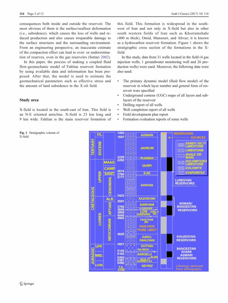
this field. This formation is widespread in the south-west of Iran and not only in X-field but also in othersouth western fields of Iran such as Khorramshahr(400 m thick), Omid, Mansouri, and Ahvaz; it is knownas a hydrocarbon reservoir formation. Figure 1 shows thestratigraphic cross section of the formations in the X-field.

In this study, data from 31 wells located in the field (4 gasinjection wells, 1 groundwater monitoring well and 26 pro-duction wells) were used. Moreover, the following data werealso used:

& The primary dynamic model (fluid flow model) of thereservoir in which layer number and general form of res-ervoir were specified

& Underground contour (UGC) maps of all layers and sub-layers of the reservoir

& Drilling report of all wells& Well completion report of all wells& Field development plan report& Formation evaluation reports of some wells

Fig. 1 Stratigraphic column ofX-field

116 Page 2 of 12 Arab J Geosci (2017) 10: 116

& Routine and Special Core Analysis data (porosity, perme-ability, fluid saturation, relative permeability, compress-ibility of rock)

& Pore pressure distribution data in the entire reservoir

Static modeling

Based on the pat te rn dis t r ibut ion of impor tantpetrophysical parameters, and also the availability of un-derground contour maps for 27 horizons of the reservoir,static model was made. The generated gridding systemincludes 38 cells along the x-axis and 83 cells along they-axis. Y-axis with an azimuth of 5° has been rotated dueto getting parallel to elongation major axis of fold. In themiddle section of the field, in which changes in all pa-rameters are more important, cell size has been decreasedrelative to adjacent cells (with proportion of 0.5). Themiddle cell size is considered 250 × 250 m. In other partsof the region, in which discretization is less important,cells are grouped for a decreasing number of cells and

the edge effect. Dimensions of this group are 250 × 300or 1000 × 1000 m. The designed networking system forthe field is illustrated in Figs. 2 and 3. Finally, the reser-voir construction model is generated with 267,260(83 × 115 × 28) cells. According to the field data, thereis no fault in this part of the field.

3D modeling of reservoir characteristics

For modeling the properties such as effective porosity,absolute permeability, water saturation, and so on, welllogging data related to those properties in all wells, whichwere calibrated using core data, are used. It is necessaryto note that effective porosity and permeability of eachwell were gained using core tests data. Actually, in thisstudy, these data were available in the corrected mode.

The Sequential Gaussian Simulation (SGS) method isused for 3D reservoir characteristics modeling. For anextensive review of other geostatistic methods, see deAlmeida (2010). Actually, among different methods forpropagating properties in three dimensions, we choosethis method because this Variogram-based method is su-perior to other methods in geoestatistic simulation of thereservoir rock properties.

Geomechanical modeling

At the beginning of 3D geomechanical modeling, one-dimensional mechanical earth models (1D MEM) were

Fig. 2 Reservoir gridding system (x- and y-axes) Fig. 3 Reservoir gridding system (x- and z-axes)

Arab J Geosci (2017) 10: 116 Page 3 of 12 116

built for 10 wells located in the field and then, the men-tioned models were used in Finite element code in orderto build the 3D geomechanical model. After that, to ex-amine the influence of the production/injection-inducedpressure changes, the three-dimensional finite differencereservoir simulations were input into three-dimensionalfinite element geomechanical simulations (Teatini et al.2014).

1D geomechanical model

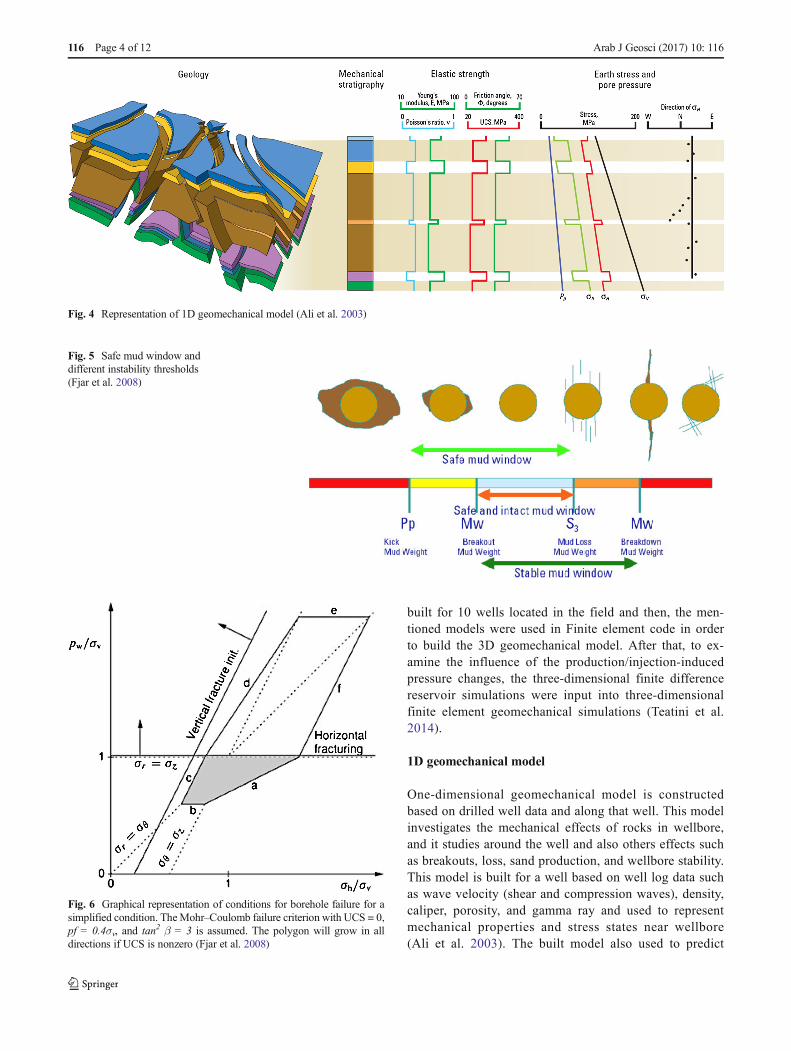
One-dimensional geomechanical model is constructedbased on drilled well data and along that well. This modelinvestigates the mechanical effects of rocks in wellbore,and it studies around the well and also others effects suchas breakouts, loss, sand production, and wellbore stability.This model is built for a well based on well log data suchas wave velocity (shear and compression waves), density,caliper, porosity, and gamma ray and used to representmechanical properties and stress states near wellbore(Ali et al. 2003). The built model also used to predict

Fig. 4 Representation of 1D geomechanical model (Ali et al. 2003)

Fig. 5 Safe mud window anddifferent instability thresholds(Fjar et al. 2008)

Fig. 6 Graphical representation of conditions for borehole failure for asimplified condition. TheMohr–Coulomb failure criterion with UCS = 0,pf = 0.4σv, and tan2 β = 3 is assumed. The polygon will grow in alldirections if UCS is nonzero (Fjar et al. 2008)

116 Page 4 of 12 Arab J Geosci (2017) 10: 116

optimal mud weight window, stability of future wells, andwell trajectories (Himmerlberg and Eckert 2013). Amongthe parameters that are represented include elastic param-eters (young, bulk and shear modulus, Poisson’s ratio),strength parameters (UCS,1 tensile strength, internal fric-tion angel, cohesion), stresses (vertical, maximum andminimum horizontal stresses), and pore pressure. An ex-ample of a 1D geomechanical model is shown in Fig. 4.

In this study, data from shear and compressional wave ve-locity and also rock mechanical tests were used to determineelastic parameters such as Young, shear and bulk modulus,Poisson ratio, cohesion, angle of internal friction, and

unconfined compressive strength (UCS) for reservoir forma-tion of Fahlian. Then, for stress condition analysis, due to thelack of stress measurement in the studied area, stress conditionwas determined based on theories and assumptions related towells. Lithostatic pressure (vertical stress) is the pressurewhich is applied by the upper layers and their weights to thelower ones. Overburden pressure in the depth of z is deter-mined using the equation below:

P zð Þ ¼ P0 þ g∫z0ρ zð Þdz ð1Þ

In which, ρ(z) is the density of overburden rocks in thedepth of z, and g is the earth acceleration. P0 is the basepressure (like pressure on the surface) (D.zobak 2007). The1 Unconfined Compressive Strength

Fig. 7 a Conditions of mainstresses, b stability thresholdlimits of well according to Fjarequations, and c an example ofappropriate fitting of designedgeomechanical model and FMIdata (well no. 10)

Arab J Geosci (2017) 10: 116 Page 5 of 12 116

c Well#10b Well#5

d

a Well#6

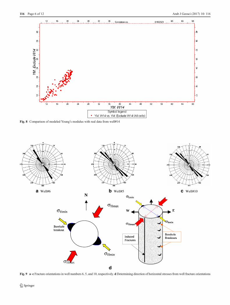
Fig. 9 a–c Fracture orientations in well numbers 6, 5, and 10, respectively. dDetermining direction of horizontal stresses fromwell fracture orientations

Fig. 8 Comparison of modeled Young’s modulus with real data from well#14

116 Page 6 of 12 Arab J Geosci (2017) 10: 116

vertical stress profile is specified based on the density of layers(Fig. 7). Knowing about the stress regime ruling, the studiedarea is very important; therefore, appropriate and accurateequations can be chosen and accurate interpretations can bepresented (Herwanger 2014). Overall, accurate information isnot available about the stress regime ruling the Fahlian reser-voir area; thus, different proportions of horizontal over vertical

stress are considered, and according to information obtainedfrom drilling, the best value was selected.

Stress condition analysis

As the most conventional condition, the regime of the area hasbeen considered as normal and horizontal stress was calculat-ed based on the following equation:

K0 ¼ σ0

h

σ0v¼ σh−Pp

σv−Ppð2Þ

σ0h ¼ kσ0

v ¼ ϑ1−ϑ

σv ð3Þ

where k is the ratio between horizontal and vertical stresses,Pp is the pore pressure, and ϑ is the Poisson ratio (D.zobak2007). In order to evaluate the resulted stress state, instabilitythreshold (usually called: kick, breakout, loss, and breakdown) should be calculated, and applied mud weight shouldbe compared with those thresholds (Fig. 5).

Among those thresholds, breakout is related to the shearfailure around the borehole. Amethod for the determination ofshear failure around boreholes was outlined by Fjar et al.(2008), which was based on the work by Guenot andSantarelli (1988). This method proposes a set of criteria,which forms a polygon (Fig. 6). This method is also appliedin the current study.

Applying the abovementioned method for different ratio ofhorizontal to vertical stress led to various results. It seems thatchoosing the exact ratio between horizontal and vertical stressis essential for the determination of possible failure around theborehole for different mud weights. Comparing the results withthe drilling report can be used as a validation method for pro-posed stress regime. As mentioned before, there is not anystress measurement records in the area. In order to study thedifferent possible stress states, different failure thresholds werecalculated for a range of ratios of horizontal to vertical stresses.According to drilling reports and image logs, noticeable fail-ures and instabilities of the ratio of horizontal to vertical stresswere assumed to be 0.6, stress regime should be normal, andvertical wells should be the most stable ones. After that, we candetermine the proportion of strains along the x- and y-axis usingEq. 2 and the maximum horizontal stress based on Eq. 3.

σh ¼ ϑ1−ϑ

σv þ 1−2ϑ1−ϑ

αPp þ E

1−ϑ2 εx þϑE

1−ϑ2 εy ð4Þ

σH ¼ ϑ1−ϑ

σv þ 1−2ϑ1−ϑ

αPp þ E

1−ϑ2 εy þϑE

1−ϑ2 εx ð5Þ

In which, Pp is the pore pressure and ϑ is the Poisson’s ratio(D.zobak 2007).

So, we have one-dimensional geomechanical model foreach well (Fig. 7 shows this model for well #10 of field).

Fig. 10 Geomechanical model networking for iterative combinedsimulation

Fig. 11 Iteratively coupling strategy between fluid flow andgeomechanical models

Arab J Geosci (2017) 10: 116 Page 7 of 12 116

3D geomechanical parameters model

Geomechanical parameters modeling such as Poisson’sratio, Young, shear and bulk modulus, and also uncon-fined compressive strength should be carried out for 3D

geomechanical modeling (Ouellet et al. 2011). As de-scribed in B1D geomechanical model^ section, we made1D mechanical earth model for 10 wells. Similar to 3Dporosity and permeability modeling, the sequentialGaussian simulation method is also used for modeling

Fig. 12 Oil production rate from Darkhovin field

Fig. 13 Cumulative value of oil production in Darkhovin field

116 Page 8 of 12 Arab J Geosci (2017) 10: 116

of the mentioned parameters in 3D space. That is whyfor each parameter, variography is carried out separatelyand also appropriate distribution functions have beenspecified for them.

In this study, the 3D geomechanical model has beenbuilt based on data from 10 wells. An example of thiscomparison between the modeled Young’s modulus andreal data in well no. 14 is presented in Fig. 8. It isnecessary to note that according to the direction of frac-tures in field wells, the minimum horizontal stress direc-tion is considered at NW-SE (Fig. 9).

Iteratively coupled fluid flow and geomechanics

Field production scenario

According to the available reports from X-field, twophases have been considered for oil production andgas injection in the development of the field. In the firstphase, wells no. 1 to 11 started producing oil from thereservoir from December 31, 2003, to December 31,2006.After that, the second phase of production withgas injection was initiated. In the second phase, gasinjection to the reservoir by wells no. 19, 21, 23, and23 was initiated. In that phase, oil was produced fromother wells except for well no. 28 which was a moni-toring well for the groundwater aquifer.

3D model preparation

After running the reservoir fluid flow simulation, theoutput related to the reservoir model was used as a textfile input for the geomechanic code, and then the codewas run for geomechanical stress and strain analysis. Inthe second coded application, which handles stress anal-ysis and subsidence estimation of the ground, reservoirgridding cells were considered greater than the primarystate for preventing edge effect on geomechanical sim-ulation (Ouellet et al. 2011). Therefore, reservoir net-working in three directions of x, y, and z has beenincreased 1.5 times (Fig. 10).

Likewise, in the geomechanical model, gridding cellshave been continued from the top of the model to theground surface (which considers flat here) and from thebottom of the model to the basement which isuncompressible.

Boundary conditions and stresses

The four lateral edges of the geomechanical model werefree to displace in all directions. The bottom of the modelwas fixed, whereas the top (i.e., earth surface) was free todisplace in all directions. The prescribed tectonic stressstate around reservoir has a significant impact on thenumerical results because of the non-linearity of the ma-terial models. Vertical stress due to gravitational loading

Fig. 14 Average reservoir pressure

Arab J Geosci (2017) 10: 116 Page 9 of 12 116

was calculated directly from the bulk density of the over-lying materials with initial pore pressures in the differentstratigraphic layers calculated as described, and also thetwo horizontal (principal) effective stresses, which areoriented parallel to the model boundaries, were previous-ly computed at each node.

Coupled model results

Fluid flow simulation in the field has been considered intwo phases, and the model execution time interval is1 month. The considered simulation running time is40 years. Thus, the last model execution time will beDecember 2043. According to the selected iterative ap-proach for the combined simulation of the geomechanicalmodel and fluid flow model, December 31, 2005, 2025,and 2043 have been considered for the geomechanicalanalysis of surface subsidence estimation. Actually, inthe mentioned dates, output of the reservoir simulationmodel will be imported to the geomechanical model asan input data, and after some analyses, geomechanicaloutputs, which are a new amount of reservoir permeabilityand porosity, will again be imported to the reservoir sim-ulation model for calculating the new pore pressure in thenext time step and also fluid flow continuation. Figure 11schematically shows linking geomechanical model andfluid flow model for iteratively coupled simulation.

Figures 12 and 13 show the field oil production rateand its cumulative value, respectively. In Fig. 14, theaverage pore pressure changes of the field are presentedover 40 years.

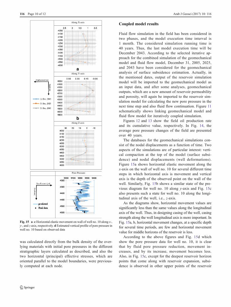
The databases for the geomechanical simulations con-sist of the nodal displacements as a function of time. Twoaspects of the simulations are of particular interest: verti-cal compaction at the top of the model (surface subsi-dence) and nodal displacements (well deformations).Figure 15a shows horizontal elastic movement along thex-axis on the wall of well no. 10 for several different timesteps in which horizontal axis is movement and verticalaxis is the depth of the observed point on the wall of thewell. Similarly, Fig. 15b shows a similar state of the pre-vious diagram for well no. 10 along y-axis and Fig. 15calso presents such a state for well no. 10 along the longi-tudinal axis of the well, i.e., z-axis.

As the diagrams show, horizontal movement values aresignificantly less than the same values along the longitudinalaxis of the well. Thus, in designing casing of the well, casingstrength along the well longitudinal axis is more important. InFig. 15a, b, horizontal movement changes, at a specific depthfor several time periods, are few and horizontal movementvalue for middle horizons of the reservoir is less.

According to the above figures and Fig. 15d whichshow the pore pressure data for well no. 10, it is clearthat by fluid pore pressure reduction, movement in-creases, and by its increase, movement becomes less.Also, in Fig. 15c, except for the deepest reservoir horizonpoints that come along with reservoir expansion, subsi-dence is observed in other upper points of the reservoir

Along X-axis

aAlong Y-axis

bAlong Z-axis

erusserPeroP

Fig. 15 a–cHorizontal elastic movement on wall of well no. 10 along x-,y-, and z-axis, respectively. d Estimated vertical profile of pore pressure inwell no. 10 based on observed data

116 Page 10 of 12 Arab J Geosci (2017) 10: 116

which is due to gas injection in the lower layers of thereservoir.

Figure 16 shows the cross section of the maximum groundsurface subsidence at the top of the reservoir in which subsi-dence value has increased by approaching the top of the res-ervoir and vice versa. Figure 17 also shows a similar state forthe longitudinal profile of the maximum ground surface sub-sidence. It is observed that ground subsidence in the study isinsignificant and maximum value equals 29 mm. The reasonconsidered can be gas injection scenario beside oil productionfrom the reservoir because gas injection can somewhat pre-vent reservoir compactness and ground subsidence. It is con-sidered that according to the obtained values of horizontaland vertical movement in the wall of different wells, thosemovements are not problematic for casing and well produc-tion and also the surrounding environment.

Conclusions

Three-dimensional finite element mechanical simulationsreveal the evolution of the subsurface stress and

displacement fields in the reservoir and overburden,and show how local production and injection patternsaffect their spatial and temporal variation. In this study,the geomechanical simulations are performed for Fahlianreservoir formation in one of the oil fields in SW ofIran. Magnitude and direction of the stress field werecalculated based on available data such as geological,geomechanical, geophysical, and reservoir engineering data.According to the constructed model, the maximum amount ofvertical and horizontal stresses is 110 and 94MPa, respective-ly. However, the 3D Sequential Gaussian Simulation (SGS)method is used for 3D reservoir characteristics modeling. Thismethod shows about 90% correlation between real data andmodel data of rock mechanics parameters such as shear oryoung modulus. From iteratively coupled fluid flow-geomechanics provided, model observed that ground subsi-dence in the study is insignificant and the maximum valueequals 29 mm. The reason considered can be the gas injectionscenario beside oil production from the reservoir because gasinjection can somewhat mitigate reservoir compaction andsurface subsidence. According to the obtained values of hor-izontal and vertical displacement in the wall of different wells,

Fig. 16 Cross section ofmaximum ground subsidence iny = 977,200

Fig. 17 Longitudinal profile ofmaximum ground subsidence inx = 1,814,000

Arab J Geosci (2017) 10: 116 Page 11 of 12 116

those are not problematic for casing and well production andalso the surrounding environment.

Open Access This article is distributed under the terms of the CreativeCommons At t r ibut ion 4 .0 In te rna t ional License (h t tp : / /creativecommons.org/licenses/by/4.0/), which permits unrestricted use,distribution, and reproduction in any medium, provided you give appro-priate credit to the original author(s) and the source, provide a link to theCreative Commons license, and indicate if changes were made.

References

Ali AHA, Brown T, DelgadoR, Lee D, PlumbD, Smirnov N,Marsden R,Prado-Velarde E, Ramsey L, Spooner D (2003) Watching rockschange—mechanical earth modeling. Oilfield Review 15(1):22–39

D.zobak M (2007) Reservoir geomechanics. Cambridge University pressde Almeida JA (2010) Stochastic simulation methods for characterization

of lithoclasses in carbonate reservoirs. Earth Sci Rev 101(3):250–270

Fjar E, Holt RM, Raaen A, Risnes R, Horsrud P (2008) Petroleum relatedrock mechanics, Elsevier

Guenot A, Santarelli F (1988) Borehole stability: a new challenge for anold problem. The 29th US Symposium on Rock Mechanics(USRMS), American Rock Mechanics Association

Herwanger J (2014) Seismic geomechanics: how to build and calibrategeomechanical models using 3D and 4D seismic data. EducationDays Stavanger 2014

Himmerlberg N, Eckert A (2013) Wellbore Trajectory Planning forComplex Stress States. 47th US Rock Mechanics/GeomechanicsSymposium, American Rock Mechanics Association

Houtenbos A (2000) The quantification of subsidence due to gas-extraction in the Netherlands. Land Subsidence, proceedings of theIAHS Sixth International Symposium On Land Subsidence(SISOLS)

Kovach RL (1974) Source mechanisms for Wilmington oil field,California, subsidence earthquakes. Bull Seismol Soc Am 64(3–1):699–711

Mayuga M (1970) Geology and development of California’s giant–Wilmington oil field

Ouellet A, Bérard T, Desroches J, Frykman P, Welsh P, Minton J,Pamukcu Y, Hurter S, Schmidt-Hattenberger C (2011) Reservoirgeomechanics for assessing containment in CO 2 storage: a casestudy at Ketzin, Germany. Energy Procedia 4:3298–3305

Settari A (2002) Reservoir compaction. J Pet Technol 54(08):62–69Sulak R (1991) Ekofisk field: the first 20 years. J Pet Technol 43(10):1,

265–261,271Teatini P, Castelletto N, Gambolati G (2014) 3D geomechanical modeling

for CO 2 geological storage in faulted formations. A case study in anoffshore northern Adriatic reservoir, Italy. International Journal ofGreenhouse Gas Control 22:63–76

116 Page 12 of 12 Arab J Geosci (2017) 10: 116