3d axon structure extraction and analysis in confocal

3D Axon Structure Extractionand Analysis in Confocal

Fluorescence Microscopy ImagesThe Harvard community has made this

article openly available. Please share howthis access benefits you. Your story matters

Citation Zhang, Yong, Xiaobo Zhou, Ju Lu, Jeff Lichtman, Donald Adjeroh, andStephen T. C. Wong. 2008. 3D axon structure extraction and analysisin confocal fluorescence microscopy images. Neural Computation20(8): 1899-1927.

Published Version doi:10.1162/neco.2008.05-07-519

Citable link http://nrs.harvard.edu/urn-3:HUL.InstRepos:12006790

Terms of Use This article was downloaded from Harvard University’s DASHrepository, and is made available under the terms and conditionsapplicable to Other Posted Material, as set forth at http://nrs.harvard.edu/urn-3:HUL.InstRepos:dash.current.terms-of-use#LAA

http://osc.hul.harvard.edu/dash/open-access-feedback?handle=&title=3D%20Axon%20Structure%20Extraction%20and%20Analysis%20in%20Confocal%20Fluorescence%20Microscopy%20Images&community=1/1&collection=1/2&owningCollection1/2&harvardAuthors=91a90f498235c600e1708486e0063247&departmentMolecular%20and%20Cellular%20Biology

http://nrs.harvard.edu/urn-3:HUL.InstRepos:12006790

http://nrs.harvard.edu/urn-3:HUL.InstRepos:dash.current.terms-of-use#LAA



ARTICLE Communicated by Sebastian Seung

3D Axon Structure Extraction and Analysis in ConfocalFluorescence Microscopy Images

Yong [email protected] [email protected] of Biomedical Informatics, Department of Radiology, The Methodist HospitalResearch Institute, Weill Cornell Medical College, Houston, TX 77030, U.S.A.

Ju [email protected] [email protected] of Molecular and Cellular Biology, Harvard University, Cambridge, MA02138, U.S.A.

Donald [email protected] Department of Computer Science and Electrical Engineering, West VirginiaUniversity, Morgantown, WV 26506, U.S.A.

Stephen T. C. [email protected] of Biomedical Informatics, Department of Radiology, Methodist HospitalResearch Institute, Weill Cornell Medical College, Houston, TX 77030, U.S.A.

The morphological properties of axons, such as their branching patternsand oriented structures, are of great interest for biologists in the studyof the synaptic connectivity of neurons. In these studies, researchers usetriple immunofluorescent confocal microscopy to record morphologicalchanges of neuronal processes. Three-dimensional (3D) microscopy im-age analysis is then required to extract morphological features of theneuronal structures. In this article, we propose a highly automated 3Dcenterline extraction tool to assist in this task. For this project, the mostdifficult part is that some axons are overlapping such that the boundariesdistinguishing them are barely visible. Our approach combines a 3D dy-namic programming (DP) technique and marker-controlled watershed al-gorithm to solve this problem. The approach consists of tracking and up-dating along the navigation directions of multiple axons simultaneously.The experimental results show that the proposed method can rapidly andaccurately extract multiple axon centerlines and can handle complicatedaxon structures such as cross-over sections and overlapping objects.

Neural Computation 20, 1899–1927 (2008) C© 2008 Massachusetts Institute of Technology

1900 Y. Zhang et al.

1 Introduction

The morphological properties of axons, such as their branching patternsand oriented structures, are of great interest to biologists who study thesynaptic connectivity of neurons. As an example, the orientation of mo-tor axons is critical in understanding synapse elimination in a developingmuscle (Keller-Peck et al., 2001). At neuromuscular junctions of developingmammals, the axonal branches of several motor neurons compete with eachother, which may result in withdrawal of all branches but one (Kasthuri &Lichtman, 2003). The 3D image reconstruction technique has been widelyused to visualize the geometrical features and topological characteristics of3D tubular biological objects to help in understanding how the morpho-logical properties of axons change during the development of the neuronalsystem.

Digital fluorescent microscopy technique offers tremendous value to lo-calize, identify, and characterize cells and molecules in brain slides andother tissues, as well as in live animals. Accordingly, microscopy imagingand image analysis would be a powerful combination that allows scientistsand researchers to gather objective, quantitative, and reproducible informa-tion, thereby obtaining stronger statistical evidence faster and with fewerexperiments. Today the bottleneck in realizing this work flow is the fullyautomated analysis of large volumes of axon images. However, it still re-mains difficult to design a fully automated image analysis algorithm dueto the limitations of computing techniques and the complexity of 3D neu-ronal images. The Vidisector (Coleman, Garvey, Young, & Simon, 1977;Garvey, Young, Simon, & Coleman, 1973) and the automatic neuron-tracingsystem (Capowski, 1989) represent early research work on the 3D neu-rite tracing problem. These methods have not been widely used due totheir poor tracing performance and frustrating use. Cohen, Roysam, andTurner (1994) proposed a tracing algorithm for 3D confocal fluorescencemicroscopy images using segmentation and skeleton extraction algorithm.He et al. (2003) extended the work of Cohen et al. using an improved skele-tonization algorithm. They combined an automatic method with semiau-tomatic and manual tracing in an interactive way in case the dendriticfragments were missed by the automatic process. Al-Kofahi et al. (2002)and Lin et al. (2005) proposed methods that are superior in terms of speedand accuracy to the work of He et al. and Cohen et al. for tracing neuritestructures by automatic seed point detection and adaptive tracing tem-plates of variable sizes. Other 3D neuron structure analysis algorithmswere based on vectorization (Can, Shen, Turner, Tanenbaum, & Roysam,1999; Andreas, Gerald, Bernd, & Werner, 1998; Shen, Roysam, Stewart,Turner, & Tanenbaum, 2001; F. Xu, Lewis, Chad, & Wheal, 1998). Thesemethods modeled the dendritic structure as cylinders, and the tracing wasconducted along these cylinders. Recently, Cai et al. (2006) proposed amethod based on repulsive snake model to extract 3D axon structures. They

Automated Extraction and Analysis of 3D Axonal Structure 1901

extended the gradient vector flow (GVF) model using repulsive force amongmultiple objects. In their method, users needed to define initial bound-aries and centerline points from the first slice. Their method performedpoorly at locations where the axons changed shape irregularly or whenthe boundaries of the axons were blurred, common cases in the test axonimages.

Many available software tools, such as NeuronJ (Meijering et al., 2004),Reconstruct (Fiala, 2006), and Imaris (Bitplane, 2006), can extract the center-lines of neuron segments in a semiautomatic manner. For instance, NeuronJcan accurately extract the centerlines of the line structures in the z-projected2D image, requiring that users manually select the starting and endingpoints. Reconstruct (Fiala, 2006), a software tool that can extract the center-lines from a 3D image volume, also requires users to manually segmentdifferent objects if they are attached or overlapped. Imaris, a commer-cial software package working interactively with the users, still requiresthat users estimate the orientation and branching patterns of the 3D ob-jects. These software tools require intensive manual segmentation of hugeamounts of 3D image data, a painstaking task that can lead to fatigue-relatedbias.

A fully automated 3D extraction and morphometry of tubelike structuresusually requires a huge amount of processing time due to the complexityand dimensionality of the 3D space. The performance is somewhat mod-erate, especially with the presence of sheetlike structures and spherelikeshapes in 3D image volumes. Sometimes researchers are interested only inparticular tubelike structures on or near a particular area, so a completeextraction of all the tubelike structures is not necessary. Another importantobservation is that it is sometimes difficult for users to select the start-ing point and the ending point for a line structure in 3D space, especiallywhen this 3D line structure is interwoven with a multitude of other 3Dline structures (see the sample images in Figure 1). We have developed asemiautomated tool to facilitate manual extraction and measurement oftubelike neuron structures from 3D image volumes. This tool is some-what similar to the 2D tracking tool proposed in Meijering et al. (2004),but for the analysis of 3D line structures in 3D image volumes. Withthis tool, users need only to interactively select an initial point for oneline structure, and then this line structure can be automatically extractedand labeled for further usage. The ending points of the 3D objects aredetected automatically by the algorithm, and thus users need not selectthese points manually. The axon geometry such as curvature and lengthcan also be measured automatically to further reduce tedious manualmeasurement process. Section 2 describes our proposed algorithm for 3Daxon structure extraction using DP and marker-controlled watershed seg-mentation. The experimental results and comparisons are presented insection 3. Section 4 concludes the article and discusses potential futurework.


Figure 1: (a) The projection view (maximum intensity projection, or MIP) ofa sample 3D axon image volume. (b) An example on how the 3D axon imagevolume is formed. The 3D axon image volume consists of a series of imagesobtained by imaging the 3D axon objects along the z-direction and projectingonto the x-y plane. Each slice contains a number of 3D axon objects projectedonto the x-y plane, as shown in the figure.

2 Method for 3D Centerline Extraction

2.1 Test Images. To record morphological changes of neuronal pro-cesses, images are acquired from neonatal mice using laser scanning im-munofluorescent confocal microscopes (Olympus Flouview FV500 and

http://www.mitpressjournals.org/action/showImage?doi=10.1162/neco.2008.05-07-519&iName=master.img-000.jpg&w=305&h=357


Bio-Rad 1024). The motor neurons expressed yellow fluorescent proteins(YFP) uniformly inside each cell. The YFP was excited with a 488 nm lineof argon laser using an X60 (1.4NA) oil objective and detected with a 520 to550 nm bandpass emission filter. Figure 1a shows the projection view (max-imum intensity projection, MIP) of one sample 3D axon image volume.Three-dimensional volumes of images of fluorescently labeled processesare obtained using a confocal microscope. Figure 1b shows an example onhow the 3D volume is formed. The left image is a 3D projection view on thex-z plan. The 3D axon image volume consists of a series of images that areobtained by imaging 3D axon objects along the z-direction and projectingonto the x-y plane. Each slice contains a number of 3D axon objects pro-jected onto the x-y plane, as shown in Figure 1. The 3D axon image containsa number of axons that are interwoven, either attached or detached, andmay go across others in the 3D space.

2.2 Image Preprocessing. In the digital imaging process, noise and ar-tifacts are frequently introduced in images, so preprocessing is usually anecessary step to remove noise and undesirable features before any furtheranalysis of images. In this project, a two-step method is used to enhancethe image quality and highlight the desired line structures. In the first step,we apply intensity adjustment to all pixels in the image. Analysis of thehistograms from the test images indicates that most images have their 8-bitintensity values in the range [0, 127]. We map the intensity values to fill theentire intensity range [0, 255] to improve image contrast.

In the second step, we apply gray-scale mathematical morphologicaltransforms to the image volume to further highlight axon objects. The mor-phological transforms are widely used in detecting convex objects in digitalimages (Meyer, 1979). The top-hat transform of an image I is

I → Itop : I − maxR

{min

R{I }} (2.1)

where Itop is top-hat transformed image and R is a structuring elementchosen to be larger than the potential convex objects in the image I . We ap-ply decomposition using periodic lines (Adams, 1993) as follows. A disk-shaped flat structuring element with a radius of 3 is used to generate adisk-shaped structuring element. Another important morphological trans-form, bottom-hat transform, can be defined in a similar way. The top-hattransform keeps the convex objects, and the bottom-hat transform containsgap areas between the objects. The contrast of the objects is maximized byadding together the top-hat transformed image and the original image andthen subtracting the bottom-hat transformed image,

J = I + Itop − Ibot, (2.2)


Figure 2: Image quality comparison for two slices using image preprocessing.For each example, the image on the top is the original slice, and the image atthe bottom is the enhanced slice.

where Ibot is the bottom-hat transformed image. Figure 2 compares theimage quality of two sample slices before and after the preprocessing.

2.3 Centerline Extraction in 3D Axon Images. We have discussed thedynamic programming (DP) technique for 2D centerline extraction in Zhanget al. (2007). Dynamic programming (Bellman & Dreyfus, 1962) is an opti-mization procedure designed to efficiently search for the global optimumof an energy function. In the field of computer vision, dynamic program-ming has been widely used to optimize the continuous problem and to findstable and convergent solutions for the variational problems (Amini, Wey-mouth, & Jain, 1990). Many boundary detection algorithms (Geiger, Gupta,Costa, & Vlontzos, 1995; Mortensen, Morse, Barrett, & Udupa, 1992) usedynamic programming as the shortest or minimum cost path graph search-ing method. The DP technique is able to extract centerlines accurately andsmoothly if both starting and ending points are specified. However, directuse of conventional DP technique is not suitable for the problem of extract-ing centerlines in 3D axon image volumes. First, given the complexity anddimensionality of a 3D image volume, it is usually difficult for users toselect the correct pair of starting-ending points. Second, due to the limita-tion of imaging resolution, some axon objects are seen overlapping (i.e., theboundaries separating them are barely visible from the slices), even thoughin reality they belong to different axon structures. If the DP search is ap-plied on such image data, it will follow the path that leads to the strongestarea, which may result in missing axon objects. Third, the DP technique iscomputationally expensive if the search is for all the optimal paths for eachvoxel in the 3D image volume.

To solve these problems, we combine the DP searching technique withmarker-controlled watershed segmentation. Our proposed method is basedon the following assumptions: (1) each axon has one, and only one, brightarea on each slice, that is, each axon goes through each slice only once;(2) the axons change directions smoothly along their navigations; (3) all the



axons start at the first slice, that is, no new axons appear during the rest ofthe slices in the 3D image volume. The satisfaction of these assumptionscan be easily observed from many 3D axon images. We consider it as ourfuture work if the 3D axon images have more complicated structures thatdo not meet the above assumptions.

Our proposed method can be briefly described as follows. The userselects a set of seed points (the center points of the search regions, alsocalled starting points), one point for each axon object, from the first slice ofthe image volume. The extraction starts from these seed points: from eachseed point, instead of searching for all the optimal paths for the entire 3-Dvolume, we dynamically search for optimal paths for the candidate pointswithin a small search region on the current slice. The search region is definedas a 10 × 10 neighborhood centered at the point estimated from the previousseed point. A cost value is calculated for each candidate point based on itsoptimal path; the point with the minimum cost value and the estimatedpoint are used as the marker, and the watershed method is applied tosegment different axon objects on the current 2D slice. The centroids ofthe segmented regions are used as the detected centerline points if certainpredefined conditions are satisfied. New searching is applied starting fromthe detected centerline points until the last slice. We provide details of themethod in the following sections.

2.3.1 Optimal Path Searching and Cost Value Calculation. In conventionalDP, searching for the optimal path involves all the neighborhoods of thecurrent point. In this project, we have assumed that axons change directionssmoothly and enter each slice only once. Thus, we can ignore the previousslice and examine only the points on the following slice. We further reducethe computation by considering only a set of neighboring points within asmall region centered at the estimated seed point. We call this region thesearch region, denoted as S. In this work, the small region has a size of 10 × 10.The size of the search region is estimated based on manual examination ofthe axon objects. That is, 10 × 10 is large enough to cover the area occupiedby one axon and where it may move on to the next slice (it can be enlargedfor applications with larger objects than ours). In general, if there are k seedpoints (that is, k axons), then there are k such small regions, and the searchregion consists of k regions: S = ⋃k

i=1 si , where si , i = 1, . . . k represents theith small 10 × 10 region.

As mentioned in section 2.3, the seed points on the first slice are manuallyselected by the user. The seed points on the other slices are estimated fromthe centerline points and tracking vector detected on the previous slice. Letq i−1 and q i represent the centerline points on the slice (i − 1) and slice (i),respectively, and �Vi−1,i represent the linking directional vector from q i−1 toq i . Then the seed points bi+1 on the slice (i + 1) are estimated as the pointsobtained by tracking from q i along the directional vector �Vi−1,i to the slice(i + 1).


Figure 3 illustrates how seed points and DP searched points are estimatedfor overlapping axon objects as well as a single axon object. The dashed ar-row lines represent the directional vectors that link the two centerline pointson the previous two slices. The points obtained by searching from the cen-terline points on the previous slice along the dashed directional vectors tothe current slice are used as the estimated seed points. The solid arrow linesrepresent the directional vectors that link the two centerline points on theprevious slice and on the current slice, which could be seen as “corrected”directional vectors for the current slice. The dashed square regions repre-sent the search regions centered at the estimated seed points. It can be seenthat these search regions are large enough to cover the axon objects.

We also illustrate the case of overlapping multiple axon objects. In thissituation, the search regions of such axon objects will have a significantoverlap. Thus, the DP search may result in a possible miss of axon objects.To address this problem, we propose marker-controlled watershed segmen-tation to distinguish overlapping axon objects. Thus, the DP searched pointscan be adjusted to the correct centerline points.

A special case is for the second slice. Since there is no linking directionalvector from the previous slice, we use the directional vector that is parallelto the z-axis to estimate the seed points on the second slice. Later in thisarticle, we show that the estimated seed points are also used as part of themarkers (see section 2.3.2).

Searching for the optimal path consists of two steps. In the first step,every point in the image volume is assigned a similarity measurement to3D line structures using the 3D line filtering method. Previous research inmodeling multidimensional line structure is exemplified by the work ofSteger et al. and Sato et al. (Haralick, Watson, & Laffey, 1983; Koller, Gerig,Szekely, & Dettwiler, 1995; Lorenz, Carlsen, Buzug, Fassnacht, & Weese,1997; Sato, Araki, Hanayama, Naito, & Tamura, 1998; Sato, Nakajima et al.,1998; Steger, 1996, 1998). In this project, the 3D line filtering is achieved byusing the Hessian matrix, a descriptor that is widely used to describe thesecond-order structures of local intensity variations around each point inthe 3D space. The Hessian matrix for a pixel p at location (x, y, z) in a 3Dimage volume I is defined as

∇2 I (p) =

Ixx(p) Ixy(p) Ixz(p)

Iyx(p) Iyy(p) Iyz(p)

Izx(p) Izy(p) Izz(p)

, (2.3)

where Ixx (p) represents the partial second-order derivative of the image atpoint p along the x direction and Iyz (p) is the partial second-order deriva-tives of the image along the y and z directions, and so on. The eigenvalues of∇2 I (p) are used to define a similarity that evaluates how close a point is to a3D line structure. Figure 4 shows the geometric relationship between three


Figure 3: Selection of marker points for (a) single axon object and (b) twoattaching axon objects. The solid arrow lines represent true tracking vectorsbetween two adjacent slices. The dashed lines represent the vectors used by thecurrent slice to estimate marker points from the previous slice. This point, DPsearched point, and the line linking them define the marker used in watershedsegmentation. Notice that since the two axon objects may be very close to eachother, the DP tracking may find centerline points that are very close or even thesame for different axon objects. This will lead to missing axons. When marker-controlled watershed segmentation is used, different axons can be distinguishedto ensure correct extraction.



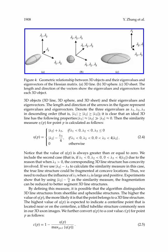
Figure 4: Geometric relationship between 3D objects and their eigenvalues andeigenvectors of the Hessian matrix. (a) 3D line. (b) 3D sphere. (c) 3D sheet. Thelength and direction of the vectors show the eigenvalues and eigenvectors foreach 3D object.

3D objects (3D line, 3D sphere, and 3D sheet) and their eigenvalues andeigenvectors. The length and direction of the arrows in the figure representeigenvalues and eigenvectors. Denote the three eigenvalues as λ1, λ2, λ3

in descending order (that is, |λ1| ≥ |λ2| ≥ |λ3|); it is clear that an ideal 3Dline has the following properties:|λ1| ≈ |λ2| � |λ3| ≈ 0. Then the similaritymeasure η (p) for point p is calculated as follows:

η(p) =

|λ2| + λ3, if λ1 < 0, λ2 < 0, λ3 ≤ 0

|λ2| − λ3

4, if λ1 < 0, λ2 < 0, 0 < λ3 < 4|λ2| .

0 otherwise

(2.4)

Notice that the value of η(p) is always greater than or equal to zero. Weinclude the second case (that is, if λ1 < 0, λ2 < 0, 0 < λ3 < 4|λ2|) due to thereason that when λ3 > 0, the corresponding 3D line structure has concavityinvolved. If we use |λ2| − λ3 to calculate the similarity measure in this case,the true line structure could be fragmented at concave locations. Thus, weneed to reduce the influence of λ3 when λ3 is large and positive. Experimentsshow that by using |λ2| − λ3

4 as the similarity measure, the fragmentationcan be reduced to better segment 3D line structures.

By defining this measure, it is possible that the algorithm distinguishes3D line structures from sheetlike and spherelike structures. The higher thevalue of η(p), the more likely it is that the point belongs to a 3D line structure.The highest value of η(p) is expected to indicate a centerline point that islocated near or on the centerline, a filled tubelike structure commonly seenin our 3D axon images. We further convert η(p) to a cost value c(p) for pointp as follows:

c(p) = 1 − η(p)maxp∈I {η(p)} . (2.5)



The value of c(p) decreases if the point goes near the centerline of the 3Dline structure, and it is minimized on the centerline.

In the second step, we search for an optimal path for each point withinthe search region on the current slice to the centerline points on the previousslice. The searching method is similar to the DP technique for 2D centerlineextraction, as described in Zhang et al. (2007). The difference is that thesearching is applied on the 3D space, and we search for the optimal pathsfor multiple axons simultaneously, not one by one. Only two slices areinvolved in the search. Thus, the processing time is significantly reduced.The cost of linking from point p to point q in the 3D space is determinedby the gradient directions of the two points. Let �dp denote the unit vectorof the gradient direction at p and �np the unit vector perpendicular to �dp.Then:

�dp = [ux(p), uy(p), uz(p)]

�np =

[uz(p), uy(p), ux(p)], if ux(p) = 0 and uy(p) = 0,[ux(p)uz(p)

uxy(p),

uy(p)uz(p)uxy(p)

,−uxy(p)]

, otherwise(2.6)

where ux(p), uy(p), uz(p) represent the unit vectors along x, y, z directionsof p, respectively. �np is obtained by rotating �dp 90 degrees counterclockwiseon the x-y plane and dividing uz (p) into two components along the x and y

directions, respectively. uxy(p) =√

u2x(p) + u2

y(p). The linking cost betweenp and q is

d(p, q ) = 23π

[cos−1 ( �np • �vpq

) + cos−1 ( �vpq • �nq)]

, (2.7)

where �vpq is the normalized bidirectional link between p and q :

�vpq =

�q − �p‖�p − �q‖; if �np • (�q − �p) ≥ 0

�p − �q‖�p − �q‖; if �np • (�q − �p) < 0

, (2.8)

where �p = [px, py, pz] and �q = [qx, qy, qz] are the vectors of the two points(p, q ) represented by their coordinates. �vpq is calculated such that the dif-ference between �p and the linking direction is minimized. The linking costbetween p and q , if calculated by formula 2.7, yields a high value if the twopoints have significantly different gradient directions or the bidirectionallink between them is significantly different from either of the two gradientdirections. The coefficient 2

3πis used to normalize the linking cost d(p, q ). It


is obtained from the fact that (1) the minimum possible angle between �vpq

and �np is 0 degree such that �np • �vpq → 0 and cos−1( �np • �vpq ) → π2 , and (2)

the maximum possible angle between �vpq and �nq is 180 degrees, such that�vpq • �nq → −1 and cos−1( �vpq • �nq ) → π . Thus, the maximum possible value

of cos−1( �np • �vpq ) + cos−1( �vpq • �nq ) is 3π2 .

The total cost value of linking point p and q can be calculated as follows:

Cost(p, q ) = wc[c(p) + c(q )] + wdd(p, q ), (2.9)

where c(p) is the local cost of p and can be calculated by formula 2.5, andd(p, q ) is the linking cost from p to q and is calculated by formula 2.7. wc, wd

are weights of local cost and linking cost, respectively. By default, wc =0.4, wd = 0.2. wc, wd are selected based on how the two factors (local costand linking cost) are expected to affect the DP search result. If the DP searchis affected more by local cost than by linking cost, then wc should increaseand wd should decrease, and vice versa, as long as condition 2wc + wd = 1is satisfied. The DP searched point for an axon object (denoted as e j for thejth slice) is selected as follows:

e j = arg minp∈S

{Cost(p, q j−1)}, (2.10)

where q j−1 denotes the jth centerline point on the jth slice. That means thatthe point with the minimum overall cost to the previous centerline point isselected as the DP searched point.

In summary, the steps of DP-based optimal path searching are as follows:

Step 1: Calculate the Hessian matrix for all image slices using formula2.3.

Step 2: Calculate the similarity measure for each point in the imagevolume using formula 2.4, and convert it to the cost value usingformula 2.5.

Step 3: Search for an optimal path for each point within the search regionon the current slice to the centerline points on the previous slice.

Step 4: Find the optimal path with minimal overall cost calculated byformula 2.9. The corresponding point is used as the DP searchedpoint and will be adjusted in the following marker-controlledwatershed, segmentation.

2.3.2 Marker-Controlled Watershed Segmentation. One difficult problemabout 3D centerline extraction is that some 3D objects may overlap orgo across others in 3D space. If two centerlines are close enough, theextraction process described may combine two centerlines as one cen-terline, and the other centerline will be completely missed (see Figure 8as an example). We address this problem by using the marker-controlled


watershed to segment different axon objects on one slice. The centroids ofsegmented regions are then used to refine the locations of the centerlinepoints.

The watershed transform has been widely used for image segmentation(Gonzalez & Woods, 2002). It treats a gray-scale image as a topographicsurface and floods this surface from its minima. If the merging of the wa-ter coming from different sources is prevented, the image is then parti-tioned into different sets: the catchment basins and the watershed linesthat separate different catchment basins. Watershed transformation hasbeen used as a powerful morphological segmentation method. It is usu-ally applied to gradient images due to the reason that the contours of agray-scale image can be viewed as the regions where the gray levels exhibitthe fastest variations, that is, the regions of maximal gradient (modulus).The major reason to use watershed transformation is that it is well suitedto the problem of separating overlapping objects (Beucher & Meyer, 1990;Dougherty, 1994; Yan, Zhao, Wang, Zelenetz, & Schwartz, 2006). Thesemethods calculate from an original image its distance transform (i.e., totransform each pixel to its minimal distance to the background). If the op-posite of the distance transform is regarded as the topological surface, thewatershed segmentation can well separate overlapping objects from theimage.

However, if the watershed transform is directly applied on gradient im-ages, it usually results in oversegmentation: the images get partitioned infar too many regions. This is mainly due to noise and inhomogeneity inimages: noise and inhomogeneity in original images result in noise andinhomogeneity in their gradient images, and this will lead to far too manyregional minima (in other words, far too many catchment basins). Themajor solution to the problem of oversegmentation is a marker-controlledwatershed, which defines new markers for the objects and floods the to-pographic surface from these markers. By doing this, the gradient functionis modified such that the only minima are the imposed markers. Thus, themost critical part of the method is how to define markers for the objects tobe extracted. In this project, for each axon object, two points can be foundautomatically: a seed point estimated from the previous image slice and aDP searched point from DP-based optimal path searching. These two pointscan be used as the object markers for watershed transform.

The marker-controlled watershed procedure in this work is as follows:

1. Calculate the gradient image from the original image slice. The mag-nitude of the image gradient at point p is calculated as follows:

|∇ I (p)| =√(

∂ I (p)∂x

)2

+(

∂ I (p)∂y

)2

. (2.11)

2. Calculate foreground markers. Foreground markers consist of esti-mated seed points, DP searched points, and the line linking them. We


Figure 5: Foreground marker selection.

involve both the estimated seed point and DP searched point as fore-ground markers to ensure that the watershed segmentation is correctif the DP searched point is located near the boundary of axon objects.Figure 5 shows how the foreground marker is selected.

3. Calculate background markers. First, the original image is segmentedinto foreground and background using a global threshold (Otsu,1979). Second, we apply distance transform to image background.Third, we apply conventional watershed transform to the result ofdistance transform and keep only the watershed ridge lines as back-ground markers.

4. Modify the gradient image so that the regional minima are at thelocations of foreground and background markers.

5. Apply marker-controlled watershed transform to the modified gra-dient image.

6. Calculate the centroids of the segmented regions, and use the resultsto adjust DP searched points to centerline points if necessary.

Let q ji denote the ith centerline point on slice ( j), e j

i denote the ith DPsearched point on slice ( j), and g j

i denote the ith centroid point on slice ( j).Then q j

i is determined as follows:

q ji =

{g j

i if∥∥g j

i − q j−1i

∥∥ ≤ εi and∥∥g j

i − e ji

∥∥ ≤ εi ,

e ji otherwise

(2.12)

where ‖g ji − q j−1

i ‖ is the 2D distance between the two points g ji and q j−1

i ,that is, the distance between two voxels if only the x-y coordinates are



considered. εi is the maximum centerline point deviation for the ith axonobject. Equation 2.12 means that if the distance between segmented centroidpoint and previous centerline point or DP searched point is within themaximum possible deviation, the centroid point will then be used as thedetected centerline point; otherwise, DP searched point will be used as thedetected centerline point. This is important in ensuring the robustness ofthe algorithm in case the watershed segmentation goes wrong on a certainslice. The value of εi is determined as

εi = max{∣∣x1

i − xZi

∣∣ , ∣∣y1i − yZ

i

∣∣}Z

(2.13)

for an image volume with Z number of slices, with each slice having asize of M × N. The values of x1

i , xZi , y1

i , yZi can be determined by manu-

ally examining the first and the last slice for each axon object in the imagevolume. In this work, we use εi = ε = maxi {εi } for simplicity. That is, theusers need to find one centerline point on the first slice and another cen-terline point on the final slice so that the two points are the farthest amongall possible pairs of centerline points. Note that the two points need notbelong to the same axon object. The total centerline deviation is obtainedby examining the coordinate difference between these two points. Then ε

is calculated as the total centerline deviation divided by total number ofslices.

It may be possible that the number of segmented regions is smaller thanthat of the axon objects after the marker-controlled watershed segmen-tation. This could happen when the global threshold calculated by Otsu(1979) is relatively high for some object regions with low-intensity values.Thus, the foreground marker may locate inside the background area. To ad-dress this problem, we iteratively reduce the threshold value to 90% of theprevious threshold value until we obtain the same number of segmentedregions as the number of axon objects, or until a predefined maximal it-eration loops. If the loop reaches the predefined maximal iteration andthe number of segmented regions is still fewer than that of previous slice,we use just the DP searched point for the missing region as the centerlinepoint.

Figure 6 illustrates the above marker-controlled watershed segmentationprocedure. Figure 6a is the original image slice, and Figure 6b gives thesegmentation result using conventional watershed. It is obvious that theimage is oversegmented. Figures 6c and 6g are the gradient images beforeand after the modification using markers. We observe that the regionalminima are better defined by the markers in Figure 6g than those in 6c.Figure 6e shows five foreground markers. These markers are obtained bydetecting five minimal cost points if connected to five centerline pointsin the preceding slice. Figure 6h gives the marker-controlled watershed


Figure 6: Example of marker-controlled watershed segmentation. (a) Origi-nal image slice. (b) Conventional watershed segmentation result. (c) Gradientimage. (d) Distance transform of image background. (e) Foreground markers.(f) Background markers. (g) Modified gradient image. (h) Marker-controlledwatershed segmentation result.

segmentation result. The five smallest regions are considered to adjust thecenterlines for the current slice.

3 Results

3.1 Three-Dimensional Axon Extraction Results. We apply our 3D cen-terline extraction algorithm on test image volumes obtained partially fromthe 3D axon images as shown in Figure 1. A typical test image volume hasa total of 512 slices (43 × 512 for each slice). Figure 7 shows three extractionresults along with 3D views of image surface rendering. The number of axonobjects in the test image volumes is 5, 6, and 4, respectively. Our method cancompletely extract all the centerlines for multiple axons in 3D space. Theextraction is accurate when the axons are overlapping or going across eachother, as shown in the figure. Figure 8 shows partial extraction results withand without marker-controlled watershed segmentation. It shows that themarker-controlled watershed helps to segment overlapping axon objects.Without watershed segmentation, DP search gives the wrong extraction atlocations where multiple axons are overlapping. Figure 9 shows extractionresults on 2D slices for overlapping multiple axons. The extracted centerline



Figure 7: 3D centerline extraction results for (a) data#116, (b) data#242,(c) data#260. The results are shown in different gray scales. For each example,the image on the top is the 3D view of the surface rendering for the originalimage; the image at the bottom is the extracted centerlines.



Figure 8: Two partial 3D centerline extraction results to show the power ofmarker-controlled watershed segmentation. (a) Surface rendering of the original3D axon image volume. (b) Extracted 3D centerlines without marker-controlledwatershed segmentation. (c) Extracted 3D centerlines with marker-controlledwatershed segmentation. Notice that the axons are overlapped at the locationindicated by arrows. We observe that one axon (indicated by dotted circles) ismissing in each example without marker-controlled watershed segmentation.

points are labeled by gray scales and are superimposed on the original im-age to show the extraction performance. Different gray scales representdifferent axon objects. Our method can accurately extract centerline pointsand distinguish different axon objects in these slices.

3.2 Result Comparison. We have tested and compared our result withthose of the repulsive snake model (Cai et al., 2006) and region-basedactive contour (RAC) method (Li, Kao, Gore, & Ding, 2007). Snakes are de-formable curves that can move and change their shape to conform to objectboundaries. The movement and deformation of snakes are controlled byinternal forces, which are intrinsic to the geometry of the snake and in-dependent of the image, and external forces, which are derived from theimage. As an extension of the conventional snake model, the gradient vec-tor flow (GVF) model (C. Xu & Prince, 1998) uses the vector field as theexternal forces such that it yields a much larger capture range than the stan-dard snake model and is much less sensitive to the choice of initialization,to improve the detection of concave boundaries. To extend the GVF modelto address the problem of 3D axon extraction, Cai et al. (2006) proposed aGVF snake model based on repulsive force among multiple objects. They



Figure 9: 3D centerline extraction results are displayed and superimposed onthe original image slices. Different gray-scale points represent centerline pointsfor different axon objects. Notice that when the axons are attaching together,our proposed method is able to accurately separate them and correctly extractthe centerline points. (a) Results for data#116. The left column shows the resultsfrom slice#97 to slice#123; the right column shows the results from slice#251 toslice#262. (b) Results for data#260. It shows the results from slice#61 to slice#83(not all the slices in the range; only typical ones are shown).

exploit the prior information of the previously separated axons and em-ploy a repulsive force to push the snakes toward their legitimate objects.The repulsive forces are obtained by reversing the gradient direction ofneighboring objects. In their method, the users need to define the initialboundaries and centerline points for the first slice. They use the final con-tour of slice n as the initialization contour for slice (n+1), assuming that the



axons do not change their positions and shapes much between consecutiveslices. Their method fails at locations where the axons change shape irreg-ularly or when the boundaries of the axons are blurred, common cases inthe test axon images. Another problem of their method is that it involvesseveral parameters that may significantly affect the extraction performance,for example, the weighting factor θ and the reliability degree d (i) used toadaptively adjust the repulsive force. Users need to iteratively adjust theseparameters in order to run the snakes, and the values may not be consistentthroughout the entire image slices.

The region-based active contour method (Li et al., 2007) is able to accu-rately segment images with noise and intensity inhomogeneity using localimage information. The local image information is obtained by introducinga kernel function of local binary fitting energy and incorporating it into avariational-level set formulation. Such a variational-level set formulationdoes not require reinitialization, which significantly reduces running time.This method, however, requires manual settings of initial contours for allthe image slices.

To compare our method with the method proposed by Cai et al. (2006)and Li et al. (2007), we carefully adjust the parameters to an optimal statefor the methods and fix them for the image volume. Since the programsprovided by Cai et al. and Li et al. only give boundaries of the detectedobjects, we assume that the centroids of the areas circled by the detectedboundaries are the detected centerline points. The results by the three meth-ods are compared in Figure 10. The test images set used are slices 53 and106 in data set #116 and slice 10 in data set #260. It shows that the repulsivesnake model cannot accurately extract axon boundaries for some slices inthe image volume; thus, the detected centerline points are not accurate.The RAC contour method can accurately extract boundaries but fails toseparate overlapping axon objects. Our method outperforms the repulsivesnake model and RAC method in both extraction performance and the re-quirement of manual initialization (it requires centerline points only on thefirst slice).

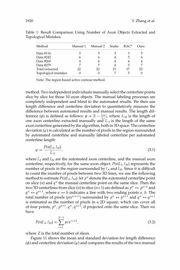
To quantitatively compare our method with the above two methods, weuse the number of topological mistakes as the measure. It is defined as thenumber of manually labeled axons minus number of automated labeledaxons. We use four full data sets to do the comparison. Table 1 showsthe number of axon objects extracted and the topological mistakes for twoindependent manual extractions, snake-based method, RAC method, andour method. It is clear that our proposed method can extract all the axonobjects seen by manual extraction.

3.3 Validation. Apart from visual inspection of the automatic resultsand manual results, we use the following experiment to quantitativelyevaluate our proposed method for 3D axon extraction. We randomly se-lect 10 different axon objects from the processed image volumes using our


Figure 10: Result comparison among our proposed method, the method by Caiet al. (2006) and the method by Li et al. (2007). From top to bottom, boundaryextraction results by Cai et al. and Li et al. and centerline point extraction resultsby our method for (a) slice 53 in dataset #116, (b) slice 10 in dataset #260, and (c)slice 106 in dataset #116. For each test result, the image on the left is obtained byCai et al.’s method; the image in the middle is obtained by Li et al.’s method; theimage on the right is obtained by our method. It is clear to see that Cai et al.’smethod performs poorly in a and b. Li et al.’s method can accurately extractboundaries but fails to separate overlapping objects, as shown in a and c.



Table 1: Result Comparison Using Number of Axon Objects Extracted andTopological Mistakes.

Method Manual 1 Manual 2 Snake RACa Ours

Data #116 5 5 3 3 5Data #242 6 6 4 5 6Data #260 4 4 4 4 4Data #279 7 7 4 5 7Total extracted 22 22 15 17 22Topological mistakes 0 0 7 5 0

Note: The region-based active contour method.

method. Two independent individuals manually select the centerline pointsslice by slice for those 10 axon objects. The manual labeling processes arecompletely independent and blind to the automated results. We then uselength difference and centerline deviation to quantitatively measure thedifference between automated results and manual results. The length dif-ference (φ) is defined as follows: φ = |1 − L M

L A|, where L M is the length of

one axon centerline extracted manually and L A is the length of the sameaxon centerline generated by the algorithm, both in 3D space. The centerlinedeviation (ϕ) is calculated as the number of pixels in the region surroundedby automated centerline and manually labeled centerline per automatedcenterline length:

ϕ = Pix(lA, lM)L A

, (3.1)

where lA and lM are the automated axon centerline, and the manual axoncenterline, respectively, for the same axon object. Pix(lA, lM) represents thenumber of pixels in the region surrounded by lA and lM. Since it is difficultto count the number of pixels between two 3D lines, we use the followingmethod to estimate Pix(lA, lM): let pn denote the automated centerline pointon slice (n) and q n the manual centerline point on the same slice. Then thetwo 3D centerlines from slice (n) to slice (n+1) are defined as pn ↔ pn+1 andq n ↔ q n+1, where a ↔ b indicates a line with two ending points a , b. Thetotal number of pixels (pixn,n+1) surrounded by pn ↔ pn+1 and q n ↔ q n+1

is estimated as the number of pixels in a 2D square, which can cover allof four points, pn, pn+1, q n, q n+1, if projected onto the same slice. Then wehave

Pix(lA, lM) =Z−1∑i=1

pixi,i+1, (3.2)

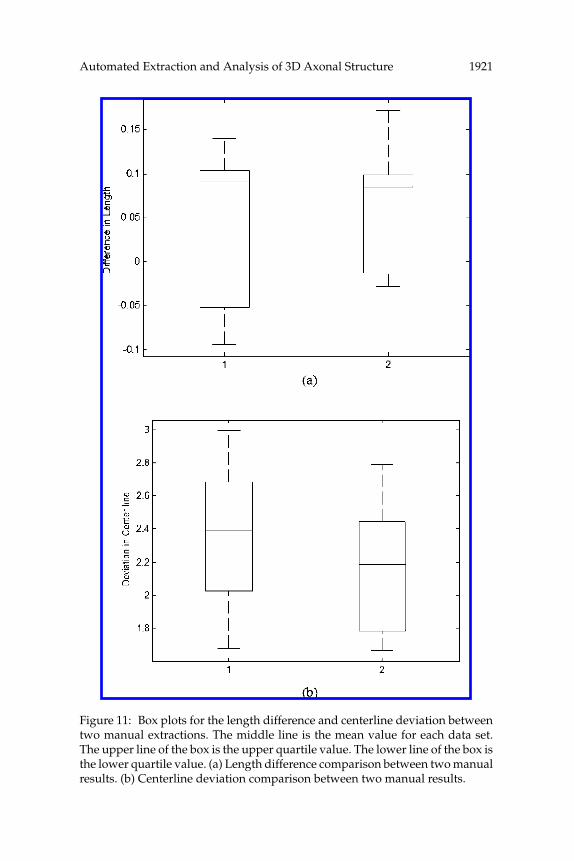
where Z is the total number of slices.Figure 11 shows the mean and standard deviation for length difference

(φ) and centerline deviation (ϕ) and compares the results of the two manual


Figure 11: Box plots for the length difference and centerline deviation betweentwo manual extractions. The middle line is the mean value for each data set.The upper line of the box is the upper quartile value. The lower line of the box isthe lower quartile value. (a) Length difference comparison between two manualresults. (b) Centerline deviation comparison between two manual results.

http://www.mitpressjournals.org/action/showImage?doi=10.1162/neco.2008.05-07-519&iName=master.img-010.png&w=277&h=451


Table 2: Mean and Standard Deviation Values for the Two Manual Results.

φ ϕ

Mean SD p-value Mean SD p-valueResult 1 0.0515 0.0861 0.3352 2.3381 0.4293 0.6661Result 2 0.0622 0.0654 2.1758 0.3686

Table 3: Pearson Linear Correlation Coefficients Among the Automated Result,the Manual Result 1, and Manual Result 2.

φ ϕ

Auto Result 1 Result 2 Auto Result 1 Result 2Auto result - 0.9873 0.9907 - - -Result 1 0.9873 - 0.9993 - - 0.9660Result 1 0.9907 0.9993 - - 0.9660 -

extractions. We can observe that the two manual results are very similar interms of φ and ϕ. Table 2 shows the values of mean and standard deviationfor φ and ϕ. We calculate the p-values of φ and ϕ using the two-sided pairedt-test and list the result in Table 2. The p-values are all greater than 0.05,which quantitatively proves that the two manual results are similar. Table 3lists the Pearson linear correlation coefficients of φ and ϕ, which shows thatthere exists a strong correlation in the automated results and the manualresults. We calculate the cumulative distribution of φ and ϕ, respectively,using Kolmogorov-Smirnov goodness-of-fit hypothesis test (Nimchinsky,Sabatini, & Svoboda, 2002) and compare the quantile-quantile plots of thetwo manual results in Figure 12. It shows a linear-like quantile-quantileplots and similar cumulative distribution functions for the three sets ofresults.

4 Conclusion

We presented a novel algorithm for extracting the centerlines of the ax-ons in the 3D space. The algorithm is able to automatically and accu-rately track multiple 3D axons in the image volume using 3D curvilin-ear structure detection. Our proposed method is able to extract centerlineand boundaries of 3D neurite structures in 3D microscopy axon images.The extraction is highly automated, rapid, and accurate, making it suit-able for replacing the fully manual methods of extracting curvilinear struc-tures when studying 3D axon images. The proposed method can handle


Figure 12: Quantile-quantile plots of the length of the axon centerlines for(a) automated versus manual result 1. (b) Automated versus manual result 2.Quantile-quantile plots of the centerline deviation for (c) manual result 1 versusmanual result 2. Cumulative distributions of the length of the axon center-lines for (d) automated (circle markers) versus manual result 1 (star markers);(e) automated (circle markers) versus manual result 2 (star markers). Cumu-lative distributions of the centerline deviation for (f) manual result 1 (circlemarkers) versus manual result 2 (star markers).

complicated axon structures such as cross-over sections and overlappingobjects.

Future work will focus on extracting more complicated axon struc-tures in the 3D space. An example of more complicated cases is shown inFigure 13. Some axon structures go through the same slice twice and maychange directions sharply. We will study a sophisticated model for extract-ing such axon structures.



Figure 13: An example 3D axon image volume with very complicated axonstructures. In this case, one axon may go across the same slice twice and maychange directions very sharply.

Acknowledgments

We thank H. M. Cai for help in testing the data sets using the programof repulsive snake model. We also thank research members (especially JunWang, Ranga Srinivasan, and Zheng Xia) of the Center for Biomedical In-formatics, Methodist Hospital Research Institute, Weill Cornell Medical



College, for their technical comments and help. The research is funded bythe Harvard NeuroDiscovery Center (formerly HCNR), Harvard MedicalSchool (Wong).

References

Adams, R. (1993). Radial decomposition of discs and spheres. Computer Vision,Graphics, and Image Processing: Graphical Models and Image Processing, 55(5), 325–332.

Al-Kofahi, K. A., Lasek, S., Szarowski, D. H., Pace, C. J., Nagy, G., Turner, J. N.,et al. (2002). Rapid automated three-dimensional tracing of neurons from confocalimage stacks. IEEE Transactions on Information Technology in Biomedicine, 6(2), 171–187.

Amini, A. A., Weymouth, T. E., & Jain, R. C. (1990). Using dynamic programmingfor solving variational problems in vision. IEEE Transactions Pattern Analysis andMachine Intelligence, 12, 855–867.

Andreas, H., Gerald, K., Bernd, M., & Werner, Z. (1998). Tracking on tree-likestructures in 3-D confocal images. In J. C. Carol, C. Jose-Angel, M. L. Jeremy,T. L. Thomas, & W. Tony (Eds.), Proceedings of the Three-Dimensional and Mul-tidimensional Microscopy: Image Acquisition and Processing V. Bellingham, WA:SPIE.

Bellman, R. E., & Dreyfus, S. E. (1962). Applied dynamic programming. Princeton, NJ:Princeton University Press.

Beucher, S., & Meyer, F. (1990). Morphological segmentation. Journal of Visual Com-munication and Image Representation, 1(1), 21–46.

Bitplane. (2006). Imaris Software. Available online at http://www.bitplane.com/products/index.shtml.

Cai, H., Xu, X., Lu, J., Lichtman, J., Yung, S. P., & Wong, S. T. C. (2006). Repulsiveforce based snake model to segment and track neuronal axons in 3D microscopyimage stacks. NeuroImage, 32, 1608–1620.

Can, A., Shen, H., Turner, J. N., Tanenbaum, H. L., & Roysam, B. (1999). Rapidautomated tracing and feature extraction from live high-resolution retinal fun-dus images using direct exploratory algorithms. IEEE Transactions on InformationTechnology in Biomedicine, 3(2), 125–138.

Capowski, J. J. (1989). Computer techniques in neuroanatomy. New York: Plenum Press.Cohen, A. R., Roysam, B., & Turner, J. N. (1994). Automated tracing and volume mea-

surements of neurons from 3-D confocal fluorescence microscopy data. Journal ofMicroscopy, 173, 103–114.

Coleman, P. D., Garvey, C. F., Young, J., & Simon, W. (1977). Semiautomatic tracing ofneuronal processes. New York: Plenum Press.

Dougherty, E. R. (1994). Digital image processing methods. Boca Raton, FL: CRC.Fiala, J. C. (2006). Reconstruct software. Available online at http://synapses.

bu.edu/tools/index.htm.Garvey, C. F., Young, J., Simon, W., & Coleman, P. D. (1973). Automated three-

dimensional dendrite tracking system. Electroencephalogr. Clin. Neurophysiol, 35,199–204.


Geiger, D., Gupta, A., Costa, L. A., & Vlontzos, J. (1995). Dynamic programmingfor detecting, tracking, and matching deformable contours. IEEE Transactions onPattern Analysis and Machine Intelligence, 17(3), 294–302.

Gonzalez, R. C., & Woods, R. E. (2002). Digital image processing. Upper Saddle River,NJ: Prentice Hall.

Haralick, R. M., Watson, L. T., & Laffey, T. J. (1983). The topographic primal sketch.International Journal of Robotics Research, 2, 50–72.

He, W., Hamilton, T. A., Cohen, A. R., Holmes, T. J., Pace, C., Szarowski, D. H.,et al. (2003). Automated three-dimensional tracing of neurons in confocal andbrightfield images. Microscopy and Microanalysis, 9, 296–310.

Kasthuri, H., & Lichtman, J. W. (2003). The role of neuronal identity in synapticcompetition. Nature, 424, 426–430.

Keller-Peck, C. R., Walsh, M. K., Gan, W.-B., Feng, G., Sanes, J. R., & Lichtman,J. W. (2001). Asynchronous synapse elimination in neonatal motor units: Studiesusing GFP transgenic mice. Neuron, 31, 381–394.

Koller, T. M., Gerig, G., Szekely, G., & Dettwiler, D. (1995). Multiscale detection ofcurvilinear structures in 2-D and 3-D image data. In Proceedings of the Fifth Inter-national Conference on Computer Vision. Washington, DC: IEE Computer Society.

Li, C., Kao, C.-Y., Gore, J. C., & Ding, Z. (2007). Implicit active contours driven bylocal binary fitting energy. In Proceedings of the IEEE Computer Society Conference onComputer Vision and Pattern Recognition. Washington, DC: IEEE Computer Society.

Lin, G., Bjornsson, C. S., Smith, K. L., Abdul-Karim, A. M., Turner, J. N., Shain, W.,et al. (2005). Automated image analysis methods for 3-D quantification of theneurovascular unit from multichannel confocal microscope images. CytometryPart A, 66A(1), 9–23.

Lorenz, C., Carlsen, I.-C., Buzug, T. M., Fassnacht, C., & Weese, J. (1997). Multi-scaleline segmentation with automatic estimation of width, contrast and tangentialdirection in 2D and 3D medical images. In Proceedings of the First Joint Conferenceon Computer Vision, Virtual Reality and Robotics in Medicine and Medial Robotics andComputer-Assisted Surgery. Berlin: Springer-Verlag.

Meijering, E., Jacob, M., Sarria, J.-C. F., Steiner, P., Hirling, H., & Unser, M. (2004).Design and validation of a tool for neurite tracing and analysis in fluorescencemicroscopy images. Cytometry, 58A(2), 167–176.

Meyer, F. (1979). Iterative image transformations for an automatic screening of cer-vical cancer. Journal of Histochemistry and Cytochemistry, 27, 128–135.

Mortensen, E., Morse, B., Barrett, W., & Udupa, J. (1992). Adaptive boundary detec-tion using “live-wire” two-dimensional dynamic programming. Paper presented atComputers in Cardiology, Durham, NC.

Nimchinsky, E. A., Sabatini, B. L., & Svoboda, K. (2002). Structure and function ofdendritic spines. Annual Review of Physiology, 64, 313–353.

Otsu, N. (1979). A threshold selection method from gray-level histograms. IEEETransactions on Systems, Man, and Cybernetics, 9(1), 62–66.

Sato, Y., Araki, T., Hanayama, M., Naito, H., & Tamura, S. (1998). A viewpointdetermination system for stenosis diagnosis and quantification in coronary an-giographic image acquisition. IEEE Transactions on Medical Imaging, 17, 121–137.

Sato, Y., Nakajima, S., Shiraga, N., Atsumi, H., Yoshida, S., Koller, T., et al. (1998).Three-dimensional multi-scale line filter for segmentation and visualization


of curvilinear structures in medical images. Medical Image Analysis, 2, 143–168.

Shen, H., Roysam, B., Stewart, C. V., Turner, J. N., & Tanenbaum, H. L. (2001).Optimal scheduling of tracing computations for real-time vascular landmarkextraction from retinal fundus images. IEEE Transactions on Information Technologyin Biomedicine, 5, 77–91.

Steger, C. (1996). Extracting curvilinear structures: A differential geometric approach.Paper presented at the Fourth European Conference on Computer Vision,Cambridge, UK.

Steger, C. (1998). An unbiased detector of curvilinear structure. IEEE Transactions onPattern Analysis and Machine Intelligence, 20(2), 113–125.

Xu, C., & Prince, J. L. (1998). Snakes, shapes, and gradient vector flow. IEEE Transac-tions on Image Processing, 7, 359–369.

Xu, F., Lewis, P. H., Chad, J. E., & Wheal, H. V. (1998). Extracting generalized cylindermodels of dendritic trees from 3D image stacks. In C. J. Cogswell, J.-A. Concello, J.M. Lerner, T. T. Lu, & T. Wilson (Eds.), Proceedings of SPIE: Three-Dimensional andMultidimensional Microscopy: Image Acquisition and Processing V. Bellingham, WA:SPIE.

Yan, J., Zhao, B., Wang, L., Zelenetz, A., & Schwartz, L. H. (2006). Marker-controlledwatershed for lymphoma segmentation in sequential CT images. Medical Physics,33(7), 2452–2460.

Zhang, Y., Zhou, X., Degterev, A., Lipinski, M., Adjeroh, D., Yuan, J., et al. (2007).Automated neurite extraction using dynamic programming for high-throughputscreening of neuron-based assays. NeuroImage, 35(4), 1502–1515.

Received May 11, 2007; accepted December 18, 2007.

This article has been cited by:

1. Erik Meijering. 2010. Neuron tracing in perspective. Cytometry Part A 9999A,NA-NA. [CrossRef]

http://dx.doi.org/10.1002/cyto.a.20895

3d axon structure extraction and analysis in confocal

Documents