3b.1 agriculture inventory elaboration part 2. 3b.2 by september 2003, 70 national communications...
TRANSCRIPT

3B.1
AGRICULTUREINVENTORY
ELABORATION
PART 2
3B.2
By September 2003, 70 national communications (NCs) from non-annex I (NAI) Parties had been compiled and assessed by the UNFCCC secretariat
According to Compilation and Synthesis reports, the problems encountered by NAI Parties in elaborating their national inventories ranked:
activity data 93 per cent emission factors 64 per cent methods 11 per cent
Status of national communications from NAI Parties

3B.3
Status of national communications from NAI Parties
NAI countries voluntarily submit their national GHG inventories and NCs
By mid-2005, 117 NAI Parties had submitted their first national communication; 3 NAI Parties had submitted their second NC; 1 NAI Party did not include its national inventory
Submitted inventories: 82 NAI Parties for 1 year (1994, mainly); 12 NAI Parties for 2 years (1990/94); 18 NAI Parties for 3–4 years; 12 NAI Parties for >4 years
100% NAI Parties included CO2; 99% included CH4 and N2O; 20% included HFCs, PFCs or SF6

3B.4
An important proportion of the problems mentioned are related to LUCF
Eliminating this sector from the analysis, the number of Parties mentioning problems decreases substantially:
Problems only with LUCF: 13 per cent (9 countries) Problems with LUCF and other sectors: 60 per cent
(42 countries) Problems, excluding mention to LUCF: 27 per cent
(19 countries)
Status of national communications from NAI Parties

3B.5
The Agriculture sector is second in terms of problems: Problems only with Agriculture: 0 per cent Problems with Agriculture and other sectors: 54 per
cent (38 countries) Problems excluding Agriculture: 46 per cent (32
countries)
Figures indicate that the Agriculture sector is less problematic – with regard to elaboration of an accurate GHG inventory – than is the LUCF sector
32 out of 70 NAI countries reported that Agriculture is not a problem (19 NAI countries reported that the LUCF sector is not a problem)
Status of national communications from NAI Parties
3B.6
INVENTORY ELABORATION
Previous activities undertaken in the framework of national GHG inventories: Preliminary key-source determination Mass balance for crop residues and animal manure Significance of sub-source categories (animal
species, anthropogenic N sources) Livestock characterization, as part of specific source
category elaboration

3B.7
INVENTORY ELABORATIONPrevious activities
Preliminary key-source determination Two ways:
Using last year’s GHG inventory data Applying tier 1 methods for all the
sectors for the year to be inventoried

3B.8
DETERMINATION OF KEY SOURCES Steps
Enumeration of source categories (SC) Ranking SC according to their emissions of CO2 equivalent Estimating individual contributions of the SC to the total
national emissions by dividing the specific contribution by total emissions and expresing the result in per cent
Calculating the accumulative contribution of the SC Key sources, added together, should account for 95% of GHG
emissions

3B.9
DETERMINATION OF KEY SOURCESCHILE, 1994 GHG inventory (Gg CO2 equivalent) (1)
SECTOR/subsector CO2- CH4 N2OTOTALS
Gg/year Gg/year Gg/year
ENERGY 36227.0 1575.2 499.1 38301.3
- ENERGY INDUSTRIES 9439.8 21.2 31.0 9492.0
- PROCESSING INDUSTRIES AND CONSTRUCTION 9255.2 33.6 31.0 9319.8
- ROAD TRANSPORT 12695.3 44.1 310.0 13049.4
- RESIDENTIAL, COMMERCIAL, INSTITUTIONAL 4049.6 606.9 124.0 4780.5
- AGRICULTURE, FORESTRY, FISHING 787.1 14.7 3.1 804.9
- C MINING<<??coal??>> 195.3 195.3
- OIL AND NATURAL GAS 659.4 659.4
- OIL REFINING, FUEL STORAGE AND DISTRIBUTION 0.0
INDUSTRIAL PROCESSES 1870.0 44.1 248.0 2162.1
- CEMENT 1021.1 1021.1
- ASPHALT 0.0
- COPPER 0.0
- GLASS 0.0
- CHEMICAL PRODUCTS 44.1 248.0 292.1
- IRON AND STEEL 812.2 812.2
- IRONALLEYS<<?iron alloys?>> 36.7 36.7
- PULP/ PAPER; FOODS/DRINKS; COOLING/OTHERS 0.0
SOLVENT USE 0.0 0.0 0.0 0.0

3B.10
DETERMINATION OF KEY SOURCES
AGRICULTURE: 0.0 6760.3 8661.3 15421.6
- RICE CULTIVATION 134.4 134.4
- ENTERIC FERMENTATION 5564.8 5564.8
- MANURE MANAGEMENT 1009.1 1304.8 2313.9
- AGRICULTURA SOILS: DIRECT EMISSIONS 4693.9 4693.9
- AGRICULTURAL SOILS: INDIRECT EMISSIONS 1495.9 1495.9
- AGRICULTURAL SOILS: PASTURE RANGE/PADDOCK 559.2 559.2
- AGRICULTURAL RESIDUE BURNING 52.0 607.5 659.5
WASTE: 0.0 1560.3 206.7 1767.0
- SEWAGE WATER TREATMENT: 3.2 3.2
- URBAN SOIL WASTES 1557.1 1557.1
- INDUSTRIAL SOLID WASTES 0.0
- UNTREATED SEWAGE WATER RUNOFF 206.7 206.7
- INDUSTRIAL LIQUID WASTES 202.9 202.9
TOTAL NATIONAL 38097.0 10142.8 9615.2 57854.9
1994 GHG inventory of Chile (Gg CO2 equivalent) (Non-energy sectors)

DETERMINATION OF KEY SOURCESKEY SOURCES FOR THE 1994 GHG-Inventory of Chile
SECTOR/sub-sector Gg/yr CO2-equiv.Contribution
SectorIndividual Cumulative
- Road transport 13049,4 22,6% 22,6% Energy
- Energy industries 9492,0 16,4% 39,0% Energy
- Processing industries and construction 9319,8 16,1% 55,1% Energy
- Enteric fermentation 5564,8 9,6% 64,7% Agriculture
- Residential, commercial, institutional 4780,5 8,3% 73,0% Energy
- Agricultural soils, direct N2O 4693,9 8,1% 81,1% Agriculture
- Urban solid wastes 1557,1 2,7% 83,8% Residues
- Agricultural soils, indirect N2O 1495,9 2,6% 86,3% Agriculture
- Manure management-N2O 1304,8 2,3% 88,6% Agriculture
- Cement 1021,1 1,8% 90,4% Energy
- Manure management-CH4 1009,1 1,7% 92,1% Agriculture
- Iron and allow 812,2 1,4% 93,5% Industrial Processes
- Agriculture, Forestry, Fishing 804,9 1,4% 94,9% Energy
- Agricultural residue burning 659,5 1,1% 96,0% Agriculture
- Oil and natural gas 659,4 1,1% 97,2% Industrial Processes
- Agricultural soils, pasture range and paddock 559,2 1,0% 98,1% Agriculture
- Chemical products 292,1 0,5% 98,7% Industrial Processes
- Waste water runoff 206,7 0,4% 99,0% Agriculture/Residues
- Industrial liquid residues 202,9 0,4% 99,4% Residues
- C mining 195,3 0,3% 99,7% Energy
- Rice production 134,4 0,2% 99,9% Agriculture
- Sewage water 3,2 0,0% 100,0% Energy
3B.12
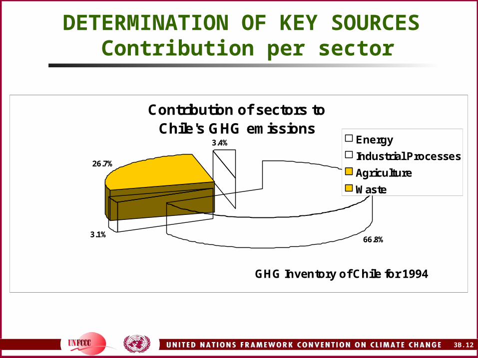
DETERMINATION OF KEY SOURCES Contribution per sector
Contribution of sectors toChile's GHG emissions
66.8%3.1%
26.7%
3.4% Energy
Industrial Processes
Agriculture
Waste
GHG Inventory of Chile for 1994

3B.13
INVENTORY ELABORATIONMass balance
Mass balance for crop residues: To be done for each crop species Example: wheat production in a country with three
agroecological units Characteristics of the agroecological units:
A: Dessert climate, agriculture only under irrigation
B: Mediterranean climate with well-marked four seasons; export agriculture under irrigation
C: Rainy and rather cold climate with no dry season; no irrigation

3B.14
INVENTORY ELABORATION Mass balance
According to experts’ judgement:
UNIT
END USE
ON-SITE OFF-SITE
TO FEED ANIMALS
INCORPORATED IN SOILS
MINERAL-IZED
BURNEDBURNED
(ENERGY)BIOGAS BRIQUETS OTHERS
A 0.00 0.00 0.00 0.50 0.45 0.00 0.00 0.05
B 0.10 0.10 0.05 0.35 0.20 0.10 0.05 0.05
C 0.25 0.20 0.20 0.20 0.00 0.15 0.00 0.00
TO BE ACCOUN-
TED UNDER
AGRICULTURAL
SOILS
CROP RESIDUES BURNING
ENERY ENERGY

3B.15
INVENTORY ELABORATIONMass balance
Factors to be applied to total wheat residues: Total wheat residues =
total productionunit i × (residue/production) factorunit i
Total residues burned in:Unit A = total residuesunit A × 0.50
Unit B = total residuesunit B × 0.35
Unit C = total residuesunit C × 0.20
3B.16
INVENTORY ELABORATIONMass balance
Mass balance for animal manure Analysis at species level First diversion, confinement and direct
grazing Second diversion, under confinement,
according to the different manure treatment systems

INVENTORY ELABORATION Mass balance
Example: non-dairy cattle population in the same country (same three agroecological units already described)
First: disaggregation of the national population in agroecological unit populations
Second: estimation of total manure produced per agroecological unit
Non-dairy cattle (experts' judgement)
UnitClimatic
conditionsDirect
grazing
Under confinement
Anaero-bic
Liquid SolidDaily
spreadOthers
Unit A Dessert 0.10 No No No 0.90 No
Unit BMediterran-
ean0.75 0.10 No 0.10 0.05 No
Unit CCold and
humid0.35 0.35 No 0.20 0.10 No
3B.17
3B.18
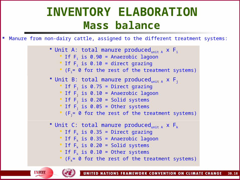
INVENTORY ELABORATION Mass balance
Manure from non-dairy cattle, assigned to the different treatment systems: Unit A: total manure producedunit A x Fi
If Fi is 0.90 = Anaerobic lagoon If Fi is 0.10 = direct grazing (Fi= 0 for the rest of the treatment systems)
Unit B: total manure producedunit A x Fj If Fj is 0.75 = Direct grazing If Fj is 0.10 = Anaerobic lagoon If Fj is 0.20 = Solid systems If Fj is 0.05 = Other systems (Fj= 0 for the rest of the treatment systems)
Unit C: total manure producedunit A x Fk If Fk is 0.35 = Direct grazing If Fk is 0.35 = Anaerobic lagoon If Fk is 0.20 = Solid systems If Fk is 0.10 = Other systems (Fk= 0 for the rest of the treatment systems)

3B.19
Significance of animal species: Example for CH4 linked to enteric fermentation and
manure management CH4 emissions estimated by tier 1 method Country as a whole, without division into
agroecological units
INVENTORY ELABORATIONSignificance of sub-sources

3B.20
Steps:
Estimation of animal species population As no national AD are available, the use of FAO
database is appropriate Disaggregation between dairy and non-dairy cattle,
following experts’ judgement Filling of Table 4-1s1 of IPCC software with the
population data and the default EFs Estimation of individual contribution to the total
emissions of the source category
INVENTORY ELABORATION Significance of sub-sources

Significance of sub-sources MODULE AGRICULTURE
SUBMODULE METHANE AND NITROUS OXIDE EMISSIONS FROM DOMESTIC LIVESTOCK
ENTERIC FERMENTATION AND MANURE MANAGEMENT
WORKSHEET 4-1
SHEET 1 OF 2 METHANE EMISSIONS FROM DOMESTIC LIVESTOCK ENTERIC
FERMENTATION AND MANURE MANAGEMENT
STEP 1 STEP 2 STEP 3
A B C D E F
Livestock Type Number of
Animals
Emissions Factor for
Enteric
Fermentation
Emissions from Enteric
Fermentation
Emissions
Factor for Manure Management
Emissions from
Manure
Management
Total Annual
Emissions from Domestic
Livestock
(1000s) (kg/head/yr) (t/yr) (kg/head/yr) (t/yr) (Gg)
C = (A x B) E = (A x D) F =(C + E)/1000
Dairy Cattle 550 81 44.550 19 10.450 55,00
Non-dairy Cattle 2750 49 134.750 13 35.750 170,50
Buffalo 0 55 0 7 0 0,00
Sheep 2500 5 12.500 0,16 400 12,90
Goats 500 5 2.500 0,17 85 2,59
Camels 125 46 5.750 1,9 237,5 5,99
Horses 75 18 1.350 1,6 120 1,47
Mules & Asses 25 10 250 0,9 22,5 0,27
Swine 5030 1 5.030 7 35.210 40,24
Poultry 15000 NE NE 0,018 270 NE
Totals 206.680 82.545 288,96
22%
65% SIGN.
<3%
6%
13%
43% SIGN.
<1%
43% SIGN.
<1%<1%<1%
<1%
<3%
<3%
<3%<3%
<1%
3B.21

3B.22
INVENTORY ELABORATION
Simulation for: Enteric fermentation – CH4 emissions
Manure management – CH4 and N2O emissions
Agricultural soils – N2O emissions
Prescribed burning of savannas – non-CO2 gas emissions
Burning of crop residues – non-CO2 gas emissions
Rice cultivation – CH4 emissions
When possible, analysis of different scenarios: Less accurate scenario: No CS activity data (usual for non-collectable
data: factors, parameters) Medium accurate scenario: No CS emission factors (very common fact) Most accurate scenario: Availability of CS activity data and emission
factors

3B.23
Enteric Fermentation

3B.24
Enteric fermentation
Hypothetical country with: Two climate regions:
Warm (60% of surface) Temperate (40% of surface)
Domestic animal population: Cattle (dairy and non-dairy) Sheep Swine Poultry Some goats and horses

3B.25
Livestock characterization
Steps: Identify and quantify existing livestock species Review emission estimation methods for each
species Identify the most detailed characterization
required for each species (i.e. ‘basic’ or ‘enhanced’)
Use same characterization for all sources (‘Enteric Fermentation’, ‘Manure Management’, ‘Agricultural Soils’)
characterization detail will depend on whether the sourcecategory is key source or not and on the relative
importance of the subcategory within the source category

3B.26
Enteric fermentation
Inventory simulation for three scenarios: 1) Low level of data availability
no access to reliable statistics or other sources of AD, and cannot use Country Specific (CS) EFs
2) Medium level of data availability detailed statistics on livestock activity, although some
Activity Data (AD2) are still required along with default/regional EFs
3) High level of data availability good country-specific AD and EFs

Low level of data availability
Species/category Number of animals (million)
Dairy cattle* 1.0
Non-dairy cattle 5.0
Buffalo 0
Sheep 3.0
Goat 0.05
Camels 0
Horses 0.01
Mules and asses 0
Swine 1.5
Poultry 4.0
Animal population data from FAO database <www.fao.org>.Open the web page; select “Statistical Databases”, “FAOSTAT-Agriculture”and “Live Animals” in Agricultural Production (searching for country,animal type and year):
* Disaggregation between dairy and non-dairy cattle based on expert’s judgement.
3B.27

3B.28
Determination of significantsub-source categories
Species contributing to 25% or more of emissions should have ‘enhanced’ characterization and tier 2 method should be applied
Perform a rough estimation of CH4 from enteric fermentation applying tier 1 method
one way of screening species for their contribution to emissions
estimation is to identify categories requiring application of tier 2 method
use IPCC software, sheet ‘4-1s1’: fill in animal population data, and collect default EF from Tables 4-3 and 4-4 of Revised 1996 IPCC Guidelines, Vol. 3 (also taken from the IPCC emission factor database (EFDB))

Determining significant animal speciesMODULE AGRICULTURE
SUBMODULE METHANE AND NITROUS OXIDE EMISSIONS FROM DOMESTIC LIVESTOCKENTERIC FERMENTATION AND MANURE MANAGEMENT
WORKSHEET 4-1
SHEET 1 OF 2 METHANE EMISSIONS FROM DOMESTIC LIVESTOCK ENTERIC FERMENTATION AND MANURE MANAGEMENT
COUNTRY Hypothetical
YEAR 2003
STEP 1 STEP 2 STEP 3A B C D E F
Livestock Type Number of Animals
Emissions Factor for
Enteric Fermentation
Emissions from Enteric Fermentation
Emissions Factor for Manure
Management
Emissions from Manure
Management
Total Annual Emissions from
Domestic Livestock
(1000s) (kg/head/yr) (t/yr) (kg/head/yr) (t/yr) (Gg)C = (A x B) E = (A x D) F =(C + E)/1000
Dairy Cattle 1000 57 57,000.00 0.00 57.00
Non-dairy Cattle 5000 49 245,000.00 0.00 245.00
Buffalo 0 55 0.00 0.00 0.00
Sheep 3000 5 15,000.00 0.00 15.00
Goats 50 5 250.00 0.00 0.25
Camels 0 46 0.00 0.00 0.00
Horses 10 18 180.00 0.00 0.18
Mules & Asses 0 10 0.00 0.00 0.00
Swine 1500 1.5 2,250.00 0.00 2.25
Poultry 4000 0 0.00 0.00 0.00
Totals 319,680.00 0.00 319.68
>25%
Worksheet 4-1s1
Conclusion: Tier 2 method, supported by an enhanced characterization, for the non-dairy cattle.
No other significant species
3B.29

3B.30
Enhanced characterization ofnon-dairy cattle population
Enhanced characterization requires information additional to that provided by FAO statistics. Consultation with local experts or industry is valuable.
Assume that (using the above information sources) the inventory team determines that the non-dairy cattle population is composed of:
Cows – 40% Steers – 40% Young growing animals – 20%
Each of these categories must have an estimate of feed intake and an EF to convert intake to CH4 emissions. Procedure is described in IPCC Good Practice Guidance and Uncertainty Management in National Greenhouse Gas Inventories (GPG2000)(pages 4.10–4.20).

Enhanced characterization of non-dairy cattle (1)
Parameter Symbol Cows Steers Young Comments
Weight (kg) W 400 450 230 Table A-2, IPCC-GL V3
Weight gain (kg/day) WG 0 0 0.3 Table A-2, IPCC-GL V3
Mature weight (kg) MW 400 450 425 Table A-2, IPCC-GL V3
Feeding situation Ca 0.28 0.23 0.25 Table 4-5 GPG2000, and expert’s judgment
Females giving birth (%)
- 67 - - Table A-2, IPCC-GL V3
Feed digestibility (%) DE 60 60 60 Table A-2, IPCC-GL V3
Maintenance coefficient
Cfi 0.335 0.322 0.322 Table 4-4 GPG2000
Net energy maintenance (MJ/day)
NEm 30.0 31.5 19.0 Calculated using equation 4.1, GPG2000
Net energy activity (MJ/day)
NEa 8.4 7.2 4.8 Calculated using equation 4.2a, GPG2000
3B.31

Enhanced characterization of non-dairy cattle (2)Parameter Symbol Cows Steers Young Comments
Growth coefficient C - - 0.9 p.4.15, GPG2000
Net energy growth (MJ/day)
NEg - - 4.0 Calculated using equation 4.3a, GPG2000
Pregnancy coefficient CP 0.1 - - Table 4.7, GPG2000
Net energy pregnancy (MJ/day)
NEP 3.0 - - Calculated using equation 4.8, GPG2000
Portion of GE that is available for maintenance
NEma/DE 0.49 0.49 0.49 Calculated using equation 4.9, GPG2000
Portion of GE that is available for growth
NEga/DE 0.28 0.28 0.28 Calculated using equation 4.10, GPG2000
Gross energy intake (MJ/day)
GE 139.3 130.4 117.7 Calculated using equation 4.11, GPG2000
To check the estimates of GE, convert to kg/day of feed intake (by dividing GE by 18.45)and divide by live weight. The result must be between 1% and 3 % of live weight.
3B.32

3B.33
Tier 2 estimation of CH4 emissions fromenteric fermentation by non-dairy cattle
Enhanced characterization yielded AD (average daily gross energy intake) for three types of non-dairy cattle
These AD must be combined with emission factors for each animal group to obtain emission estimates
Determination of EFs requires selection of a suitable value for methane conversion rate (Ym) In this example (country with no CS data) a default
value for Ym can be obtained from GPG2000
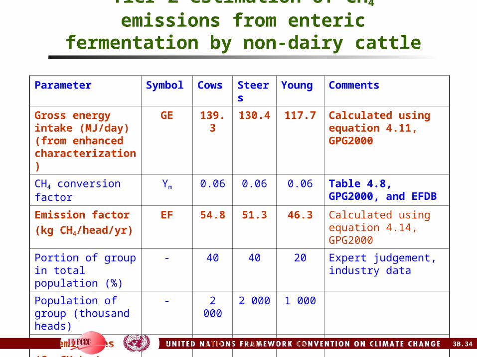
Tier 2 estimation of CH4 emissions from enteric fermentation by non-dairy cattle
Parameter Symbol Cows Steers Young Comments
Gross energy intake (MJ/day) (from enhanced characterization)
GE 139.3 130.4 117.7 Calculated using equation 4.11, GPG2000
CH4 conversion factor
Ym 0.06 0.06 0.06 Table 4.8, GPG2000, and EFDB
Emission factor
(kg CH4/head/yr)
EF 54.8 51.3 46.3 Calculated using equation 4.14, GPG2000
Portion of group in total population (%)
- 40 40 20 Expert judgement, industry data
Population of group (thousand heads)
- 2 000 2 000 1 000
CH4 emissions
(Gg CH4/yr)
- 110 103 46
3B.34

3B.35
Tier 2 estimation of CH4 emissions from enteric fermentation by non-dairy cattle
Tier 2 estimation for non-dairy cattle: 259 Gg CH4 (against 245 Gg CH4 for tier 1)
Weighted EF: 52 kg CH4/head/yr (againts the default value
of 49 kg CH4/head/yr) This value should be used in the worksheet to
report emissions by non-dairy cattle

3B.36
Medium level of data availability
Assume that the country has good statistics on livestock populations
Applying the same procedure as in previous example, the country determines that non-dairy cattle category requires enhanced characterization
National statistics + expert judgement allow disaggregation of non-dairy cattle population by:
Two climate regions Three systems of production Three animal categories (same as in previous example)

Medium Level of Data Availability
Climate region
Production system
Population (thousand heads)
Cows Steers Young
Warm Extensive grazing
1 473 828 610
Intensive grazing 228 414 120
Feedlot 40 92 96
Temperate Extensive grazing
348 201 161
Intensive grazing 150 275 75
Feedlot 15 31 32
Total - 2 254 1 841 1 094
New total: 5,153,000 heads (against FAO: 5,000,000 heads).
3B.37
3B.38
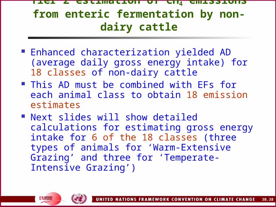
Tier 2 estimation of CH4 emissions from enteric fermentation by non-dairy cattle
Enhanced characterization yielded AD (average daily gross energy intake) for 18 classes of non-dairy cattle
This AD must be combined with EFs for each animal class to obtain 18 emission estimates
Next slides will show detailed calculations for estimating gross energy intake for 6 of the 18 classes (three types of animals for ‘Warm-Extensive Grazing’ and three for ‘Temperate-Intensive Grazing’)

Enhanced characterization, non-dairy cattleWarm Climate, Extensive Grazing (1)
Parameter Symbol Cows Steers Young Comments
Weight (kg) W 420 380 210 Country-specific data
Weight gain (kg/day) WG 0 0.2 0.2 Country-specific data
Mature weight (kg) MW 420 440 430 Country-specific data
Feeding situation Ca 0.33 0.33 0.33 Table 4-5 GPG2000, and expert judgement
Females giving birth (%) - 60 - - Country-specific data
Feed digestibility (%) DE 57 57 57 Country-specific data
Maintenance coefficient Cfi 0.335 0.322 0.322 Table 4-4 GPG2000
Net energy maintenance (MJ/day)
NEm 31.1 27.7 17.8 Calculated using equation 4.1, GPG2000
Net energy activity (MJ/day)
NEa 10.3 9.2 5.9 Calculated using equation 4.2a, GPG2000
Comments in green indicate improvements over previous example.
3B.39

Enhanced characterization, non-dairy cattleWarm Climate, Extensive Grazing (2)
Parameter Symbol Cows Steers Young Comments
Growth coefficient C - 1.0 0.9 p.4.15, GPG2000
Net energy growth (MJ/day) NEg - 3.4 2.4 Calculated using equation 4.3a, GPG2000
Pregnancy coefficient CP 0.1 - - Table 4.7, GPG2000
Net energy pregnancy (MJ/day)
NEP 3.1 - - Calculated using equation 4.8, GPG2000
Portion of GE availablefor maintenance
NEma/DE 0.48 0.48 0.48 Calculated using equation 4.9, GPG2000
Portion of GE available for growth
NEga/DE 0.26 0.26 0.26 Calculated using equation 4.10, GPG2000
Gross energy intake (MJ/day)
GE 162.2 170.0 111.2 Calculated using equation 4.11, GPG2000
To check estimates of GE, convert to kg/day of feed intake (by dividing GE by 18.45)and divide by live weight. The result must be between 1 and 3 % of live weight.
3B.40

Enhanced characterization, Non-Dairy Cattle, Temperate Climate, Intensive Grazing (1)
Parameter Symbol Cows Steers Young Comments
Weight (kg) W 405 390 240 Country-specific data
Weight gain (kg/day) WG 0.15 0.33 0.65 Country-specific data
Mature weight (kg) MW 445 470 452 Country-specific data
Feeding situation Ca 0.17 0.17 0.17 Table 4-5 GPG2000, and expert judgement
Females giving birth (%) - 81 - - Country-specific data
Feed digestibility (%) DE 72 72 72 Country-specific data
Maintenance coefficient Cfi 0.335 0.322 0.322 Table 4-4 GPG2000
Net energy maintenance (MJ/day)
NEm 30.2 28.3 19.6 Calculated using equation 4.1, GPG2000
Net energy activity (MJ/day)
NEa 5.1 4.8 3.3 Calculated using equation 4.2a, GPG2000
Comments in green indicate improvements over previous example.
3B.41

Enhanced characterization, Non-Dairy Cattle, Temperate Climate, Intensive Grazing (2)
Parameter Symbol Cows Steer Young Comments
Growth coefficient C 0.8 1.0 0.9 p.4.15, GPG2000
Net Energy Growth (MJ/day)
NEg 3.0 5.7 9.2 Calculated using equation 4.3a, GPG2000
Pregnancy coefficient CP 0.1 - - Table 4.7, GPG2000
Net Energy Pregnancy (MJ/day)
NEP 3.0 - - Calculated using equation 4.8, GPG2000
Portion of GE that is available for maintenance
NEma/DE 0.53 0.53 0.53 Calculated using equation 4.9, GPG2000
Portion of GE that is available for growth.
NEga/DE 0.34 0.34 0.34 Calculated using equation 4.10, GPG2000
Gross Energy Intake (MJ/day)
GE 120.1 123.9 121.5 Calculated using equation 4.11, GPG2000
To check estimates of GE, convert to kg/day of feed intake (by dividing GE by 18.45)and divide by live weight. The result must be between 1 and 3 % of live weight.
3B.42

3B.43
Medium level of data availability
Estimated GE values are used for calculation of EF (using equation 4.14, GPG2000)
Calculation of EF required to select a value for methane conversion rate (Ym), that is, the fraction of energy in feed intake that is converted to energy in methane
In this example we assume the country uses a default value (Ym =0.06, from Table 4.8, GPG2000)
18 estimates of EF were obtained (next slide)

Medium level of data availability
Climate region
Production system
EF (kg CH4/head/yr)
Cows Steers Young
Warm Extensive grazing
63.8 66.9 43.8
Intensive grazing 47.7 51.5 48.4
Feedlot 41.5 49.3 52.8
Temperate Extensive grazing
61.5 66.7 49.5
Intensive grazing 47.3 48.8 47.8
Feedlot 41.5 49.3 52.8
3B.44
3B.45
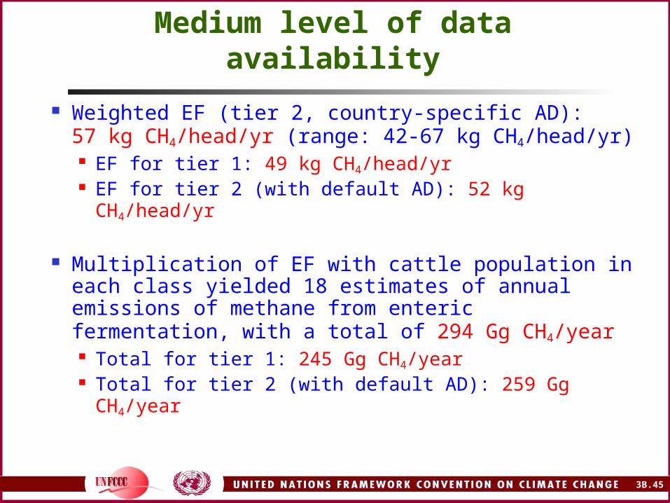
Medium level of data availability
Weighted EF (tier 2, country-specific AD):57 kg CH4/head/yr (range: 42-67 kg CH4/head/yr) EF for tier 1: 49 kg CH4/head/yr EF for tier 2 (with default AD): 52 kg CH4/head/yr
Multiplication of EF with cattle population in each class yielded 18 estimates of annual emissions of methane from enteric fermentation, with a total of 294 Gg CH4/year Total for tier 1: 245 Gg CH4/year Total for tier 2 (with default AD): 259 Gg CH4/year
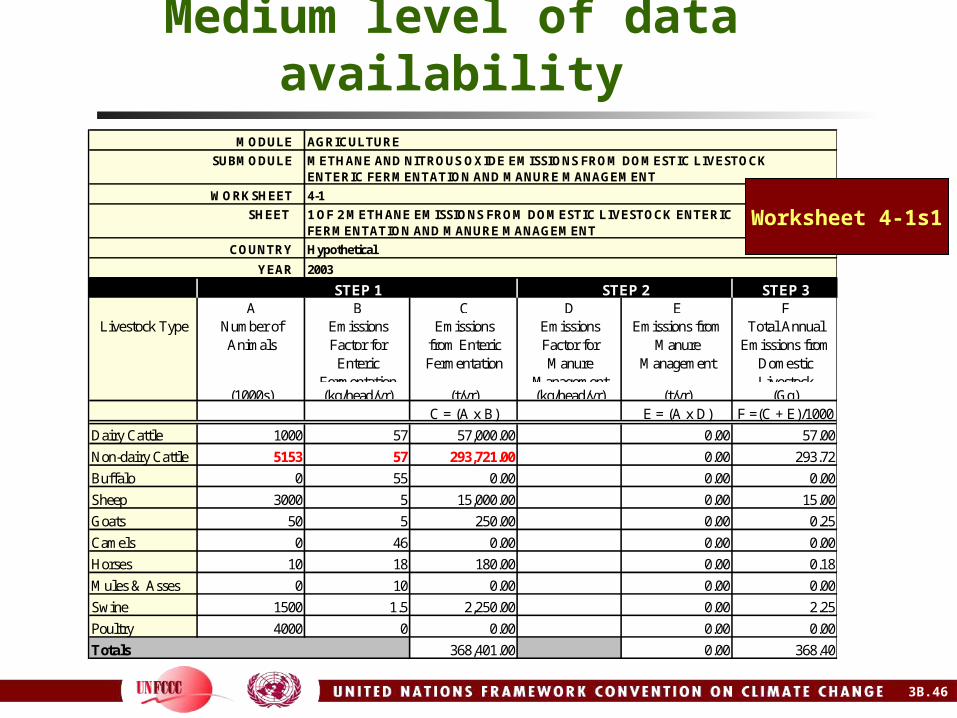
Medium level of data availabilityMODULE AGRICULTURE
SUBMODULE METHANE AND NITROUS OXIDE EMISSIONS FROM DOMESTIC LIVESTOCKENTERIC FERMENTATION AND MANURE MANAGEMENT
WORKSHEET 4-1
SHEET 1 OF 2 METHANE EMISSIONS FROM DOMESTIC LIVESTOCK ENTERIC FERMENTATION AND MANURE MANAGEMENT
COUNTRY Hypothetical
YEAR 2003
STEP 1 STEP 2 STEP 3A B C D E F
Livestock Type Number of Animals
Emissions Factor for
Enteric Fermentation
Emissions from Enteric Fermentation
Emissions Factor for Manure
Management
Emissions from Manure
Management
Total Annual Emissions from
Domestic Livestock
(1000s) (kg/head/yr) (t/yr) (kg/head/yr) (t/yr) (Gg)C = (A x B) E = (A x D) F =(C + E)/1000
Dairy Cattle 1000 57 57,000.00 0.00 57.00
Non-dairy Cattle 5153 57 293,721.00 0.00 293.72
Buffalo 0 55 0.00 0.00 0.00
Sheep 3000 5 15,000.00 0.00 15.00
Goats 50 5 250.00 0.00 0.25
Camels 0 46 0.00 0.00 0.00
Horses 10 18 180.00 0.00 0.18
Mules & Asses 0 10 0.00 0.00 0.00
Swine 1500 1.5 2,250.00 0.00 2.25
Poultry 4000 0 0.00 0.00 0.00
Totals 368,401.00 0.00 368.40
Worksheet 4-1s1
3B.46

3B.47
Highest level of data availability
Activity data could be improved by: more accurate national statistics on livestock population and
uncertainties further disaggregation of cattle population (e.g. by race and
animal age, or by subdividing climate region by administrative units, soil type, forage quality, etc.)
implementation of geographically explicit AD and cattle traceability systems
development of local research to obtain better estimates of parameters used for livestock characterization(e.g. coefficients for maintenance, growth, activity or pregnancy)

3B.48
Highest level of data availability
EFs could be improved by: developing local capacities for measuring CH4
emissions by cattle characterizing diverse feeds by their CH4
conversion factors for different animal types development of local research to improve
understanding of locally relevant factors affecting methane emissions
adapting international information (scientific literature, EFDB, etc.) from areas with conditions similar to those of the country

3B.49
Highest level of data availability
Numerical example not developed here
Few, if any, developing countries are currently in the position of having access to this level of information
With high level of data availability, countries would be able to implement tier 3 methods (still not proposed by IPCC)

Example of development of local capacity in Uruguay
Almost 50% of GHG emissions in Uruguay come from enteric fermentation
A project was implemented by the National Institute of Agricultural Research co-funded by US-EPA to improve local capacity to measure CH4
First results indicate that IPCC default EF used so far in preparation of inventories may be too high
A similar project is being conducted in Brazil by EMBRAPA
3B.50

3B.51
Estimation of Uncertainties
It is good practice to estimate and report uncertainties of emission estimates, which implies estimating uncertainties of AD and EF
According to IPCC, EFs used in a tier 1 method might have an uncertainty of 30–50%, and default AD might have even higher values
Application of a tier 2 method with country-specific AD can substantially reduce uncertainty levels compared to a tier 1 method with default AD/EF
Priority should be given to improve the quality of AD estimates
3B.52
Manure Management:CH4 Emissions

3B.53
Manure management – CH4
We will continue with the assumptions relating to the same hypothetical country
Again, tier 1 method will be applied to assess the significance of the different species for this source category
with the purpose of identifying the need for enhanced characterization
in practice, this should be done as a first step in inventory elaboration, considering that it is good practice to use the same characterization for all categories (it is presented here for training purposes only)
Numerical examples for countries with different levels of data availability will be developed
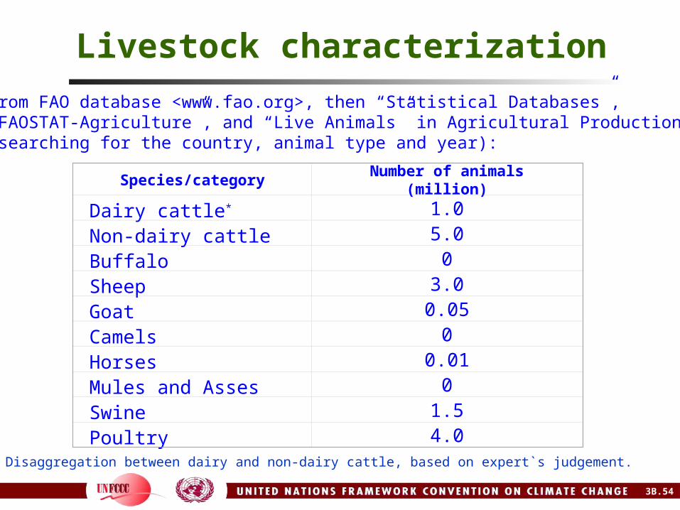
Livestock characterization
Species/category Number of animals (million)
Dairy cattle* 1.0
Non-dairy cattle 5.0
Buffalo 0
Sheep 3.0
Goat 0.05
Camels 0
Horses 0.01
Mules and Asses 0
Swine 1.5
Poultry 4.0
From FAO database <www.fao.org>, then “Statistical Databases”, “FAOSTAT-Agriculture”, and “Live Animals” in Agricultural Production(searching for the country, animal type and year):
* Disaggregation between dairy and non-dairy cattle, based on expert`s judgement.
3B.54

Livestock characterization
MODULE AGRICULTURE
SUBMODULE METHANE AND NITROUS OXIDE EMISSIONS FROM DOMESTIC LIVESTOCKENTERIC FERMENTATION AND MANURE MANAGEMENT
WORKSHEET 4-1
SHEET 1 OF 2 METHANE EMISSIONS FROM DOMESTIC LIVESTOCK ENTERIC FERMENTATION AND MANURE MANAGEMENT
COUNTRY Hypothetical
YEAR 2003
STEP 1 STEP 2 STEP 3A B C D E F
Livestock Type Number of Animals
Emissions Factor for
Enteric Fermentation
Emissions from Enteric Fermentation
Emissions Factor for Manure
Management
Emissions from Manure
Management
Total Annual Emissions from
Domestic Livestock
(1000s) (kg/head/yr) (t/yr) (kg/head/yr) (t/yr) (Gg)C = (A x B) E = (A x D) F =(C + E)/1000
Dairy Cattle 1000 57 57,000.00 1.6 1,600.00 58.60
Non-dairy Cattle 5153 57 293,721.00 1.6 8,244.80 301.97
Buffalo 0 55 0.00 1.6 0.00 0.00
Sheep 3000 5 15,000.00 0.196 588.00 15.59
Goats 50 5 250.00 0.2 10.00 0.26
Camels 0 46 0.00 2.32 0.00 0.00
Horses 10 18 180.00 1.96 19.60 0.20
Mules & Asses 0 10 0.00 1.08 0.00 0.00
Swine 1500 1.5 2,250.00 1.6 2,400.00 4.65
Poultry 4000 0 0.00 0.021 84.00 0.08
Totals 368,401.00 12,946.40 381.35
Worksheet 4-1s1
Significantspecies
3B.55

3B.56
Livestock characterization
The non-dairy cattle sub-source is the most significant, and deserves enhanced characterization and application of a tier 2 method for CH4 from manure management
Swine account for 20% of total emissions, and the country considers it appropriate to develop an enhanced characterization and apply a tier 2 method for this species as well
3B.57
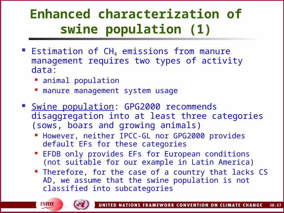
Enhanced characterization of swine population (1)
Estimation of CH4 emissions from manure management requires two types of activity data:
animal population manure management system usage
Swine population: GPG2000 recommends disaggregation into at least three categories (sows, boars and growing animals)
However, neither IPCC-GL nor GPG2000 provides default EFs for these categories
EFDB only provides EFs for European conditions (not suitable for our example in Latin America)
Therefore, for the case of a country that lacks CS AD, we assume that the swine population is not classified into subcategories

3B.58
Enhanced characterization of swine population (2)
Manure management system (MMS): we make the following assumptions for the inventory simulation for a country lacking CS AD: swine population is equally distributed among the
two climate regions (i.e. 60% in warm area, 40% in temperate area)
90% of manure is managed as a solid 10% is managed in liquid-based systems it is not possible to discriminate between MMS by
climate regions

3B.59
Low level of data availability: CH4 emissions by non-dairy cattle, swine
Tier 2 method requires determination of three parameters to estimate EF: VS (kg): mass of volatile solids excreted Bo (m3/kg of VS): max. CH4 producing capacity; MCF: CH4 conversion factor
For low level of data: default AD derived from FAO database and expert
judgement. default EF from IPCC-GL and GPG2000
Examples for non-dairy cattle, swine in next slides

Low level of data availability: CH4 emissions frommanure management for non-dairy cattle (default AD and EF) (1)
Parameter Symbol Cows Steers Young Comments
Gross energy intake (MJ/day)
(from the enhanced characterization)
GE 139.3 130.4 117.7 Calculated using equation 4.11, GPG2000 *
Energy intensity of feed (MJ/kg)
- 18.45 18.45 18.45 IPCC default value
Feed intake
(kg dm/day)
- 7.55 7.07 6.38 Calculated
Feed digestibility (%) DE 60 60 60 Table A-2, IPCC-GL V3
Ash content of manure (%)
ASH 8 8 8 IPCC-GL V3, p. 4.23
Volatile solid excretion (kg dm/day)
VS 2.78 2.60 2.35 Calculated using equation 4.16, GPG2000
Maximum CH4 producing capacity of manure (m3CH4/kg VS)
Bo 0.10 0.10 0.10 Table B-1, p.4.40,IPCC-GL V3
*GE is used for determining VS. If these data are not available, default VS values are provided in Table B-1, p. 4.40 IPCC-GL.
3B.60

Low level of data availability: CH4 emissions frommanure management for non-dairy cattle (default AD and EF) (2)
Parameter Symbol Cows Steer Young Comments
Methane conversion factor (%)
MCF 1.8 1.8 1.8 Table 4-8, p.4.25, IPCC-GL V3 (data for pasture/range/paddock system, weighted by climate region)
Emission factor
(kg CH4/head/yr)
EF 1.22 1.14 1.03 Calculated using equation 4.17, GPG2000
Population (thousand heads)
- 2 000 2 000 1 000 FAO database, local experts, industry
CH4 emissions
(Gg CH4 /yr)
- 2.45 2.29 1.03 Total emissions:
5.8 Gg CH4 /yr
Total emissions estimated here are lower than those using Tier 1 (8.2 Gg CH4/yr).Weighted EF derived from this table is 1.2 kg CH4/head/yr, and this value should be usedinstead of the default (1.6 kg CH4/head/yr) in IPCC Software
3B.61

Low level of data availability: CH4 emissions frommanure management for Swine (default AD and EF) (1)
Parameter Symbol Warm solid
Warm liquid
Temp.
solid
Temp.
liquidComments
Gross energy intake (MJ/day)
(from the enhanced characterization)
GE 13.0 13.0 13.0 13.0 Default value, Table B-2, p. 4.42, IPCC-GL V3
Energy intensity of feed (MJ/kg)
- 18.45 18.45 18.45 18.45 IPCC default value
Feed intake
(kg dm/day)
- 0.7 0.7 0.7 0.7 Calculated
Feed digestibility (%) DE 50 50 50 50 IPCC-GL V3, p. 4.23
Ash content of manure (%)
ASH 8 8 8 8 IPCC-GL V3, p. 4.23
Volatile solid excretion (kg dm/day)
VS 0.34 0.34 0.34 0.34 Calculated using equation 4.16, GPG2000
Max. CH4 producing capacity of manure (m3CH4/kg VS)
Bo 0.29 0.29 0.29 0.29 Table B-2, p.4.42, IPCC-GL V3
3B.62

Low level of data availability: CH4 emissions frommanure management for Swine (default AD and EF) (2)
Parameter Symbol Warm
solid
Warm
liquid
Temp
solid
Temp
liquidComments
Methane conversion factor (%)
MCF 2 65 1.5 35 Table 4-8, p.4.25, IPCC-GL V3 *
Emission factor
(kg CH4/head/yr)
EF 0.5 15.6 0.4 8.4 Calculated using equation 4.17, GPG2000
Population (thousand heads)
- 810 90 540 60 FAO Database, local experts, industry
CH4 emissions
(Gg CH4 /yr)
- 0.39 1.40 0.19 0.50 Total emissions:
2.5 Gg CH4 /yr
Total emissions estimated were similar to those using tier 1 (2.4 Gg CH4/yr).Weighted EF derived from this table is 1.7 kg CH4/head/yr, and this value should beused instead of the default (1.6 kg CH4/head/yr) in IPCC Software,
* Liquid/slurry was assumed to be the only system used. GPG2000 provides slightlydifferent default values (Table 4.10), as well as a formula for accounting for recovery,flaring, and use of biogas.
3B.63

Low level of data availability: resultsMODULE AGRICULTURE
SUBMODULE METHANE AND NITROUS OXIDE EMISSIONS FROM DOMESTIC LIVESTOCKENTERIC FERMENTATION AND MANURE MANAGEMENT
WORKSHEET 4-1
SHEET 1 OF 2 METHANE EMISSIONS FROM DOMESTIC LIVESTOCK ENTERIC FERMENTATION AND MANURE MANAGEMENT
COUNTRY Hypothetical
YEAR 2003
STEP 1 STEP 2 STEP 3A B C D E F
Livestock Type Number of Animals
Emissions Factor for
Enteric Fermentation
Emissions from Enteric Fermentation
Emissions Factor for Manure
Management
Emissions from Manure
Management
Total Annual Emissions from
Domestic Livestock
(1000s) (kg/head/yr) (t/yr) (kg/head/yr) (t/yr) (Gg)C = (A x B) E = (A x D) F =(C + E)/1000
Dairy Cattle 1000 57 57,000.00 1.6 1,600.00 58.60
Non-dairy Cattle 5153 57 293,721.00 1.2 6,183.60 299.90
Buffalo 0 55 0.00 1.6 0.00 0.00
Sheep 3000 5 15,000.00 0.196 588.00 15.59
Goats 50 5 250.00 0.2 10.00 0.26
Camels 0 46 0.00 2.32 0.00 0.00
Horses 10 18 180.00 1.96 19.60 0.20
Mules & Asses 0 10 0.00 1.08 0.00 0.00
Swine 1500 1.5 2,250.00 1.7 2,550.00 4.80
Poultry 4000 0 0.00 0.021 84.00 0.08
Totals 368,401.00 11,035.20 379.44
3B.64

3B.65
Medium level of data availability
Assume the country has good statistics on livestock population to develop an enhanced characterization with CS AD, but has to use default EFs
Non-Dairy Cattle: Same 18 classes as for enteric fermentation
Assume that 50% of manure from feedlot has liquid/slurry management system, and 50% anaerobic lagoons
Swine: 18 classes are identified and quantified, based on combination of:
Two climate regions Three manure management systems Three swine population categories

Medium level of data availability (Swine)
Climate region
Manure management
system
Population (thousand heads)
Sows Boars Young
Warm Pasture/range/paddock
121 30 490
Liquid/slurry 8 3 40
Anaerobic lagoon 2 2 9
Temperate Pasture/range/paddock
130 36 555
Liquid/slurry 5 1 24
Anaerobic lagoon 8 1 40
Total - 274 73 1 158
New Total: 1,505,000 heads (FAO: 1,500,000)
3B.66

3B.67
Tier 2 estimation of CH4 from manure management by non-dairy cattle, swine
Next slides will show examples of detailed calculations for tier 2 method estimation of CH4 emissions from manure management by:
Non-dairy cattle under ‘Warm Region–Extensive Grazing’ system
Swine under ‘Temperate–Liquid/Slurry’ system
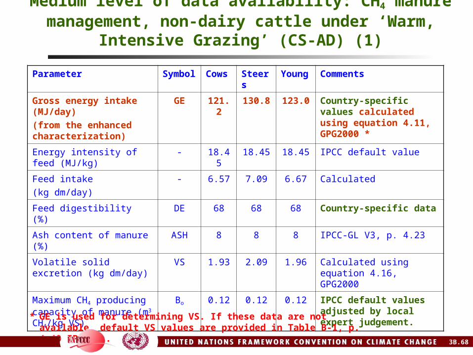
Medium level of data availability: CH4 manure management, non-dairy cattle under ‘Warm, Intensive Grazing’ (CS-AD) (1)
Parameter Symbol Cows Steers Young Comments
Gross energy intake (MJ/day)
(from the enhanced characterization)
GE 121.2 130.8 123.0 Country-specific values calculated using equation 4.11, GPG2000 *
Energy intensity of feed (MJ/kg)
- 18.45 18.45 18.45 IPCC default value
Feed intake
(kg dm/day)
- 6.57 7.09 6.67 Calculated
Feed digestibility (%) DE 68 68 68 Country-specific data
Ash content of manure (%) ASH 8 8 8 IPCC-GL V3, p. 4.23
Volatile solid excretion (kg dm/day)
VS 1.93 2.09 1.96 Calculated using equation 4.16, GPG2000
Maximum CH4 producing capacity of manure (m3
CH4/kg VS)
Bo 0.12 0.12 0.12 IPCC default values adjusted by local expert judgement.
* GE is used for determining VS. If these data are not available, default VS values are provided in Table B-1, p. 4.40 IPCC-GL.
3B.68

Medium level of data availability: CH4 manure management, non-dairy cattle under ‘Warm, Intensive Grazing’ (CS-AD) (2)
Parameter Symbol Cows Steers Young Comments
Methane conversion factor (%)
MCF 2.0 2.0 2.0 Table 4-8, p.4.25, IPCC-GL V3
Emission factor
(kg CH4/head/yr)
EF 1.14 1.23 1.15 Calculated using equation 4.17, GPG2000
Population (thousand heads)
- 228 414 120 Country-specific data
CH4 emissions
(Gg CH4 /yr)
- 0.26 0.51 0.14
In this case, the country has its own estimation for feed/gross energy intake, feed digestibility, and animal population for each of the different classes of non-dairy cattle.For Bo, even though the country has no locally developed studies, IPCC default was adjusted for local conditions following expert judgement. For other factors (ASH, MCF), IPCC default values were used.
3B.69

Medium level of data availability: CH4 manure management, swine under ‘Warm, Liquid/Slurry’ (CS-AD) (1)
Parameter Symbol Sows Boars Young Comments
Gross energy intake (MJ/day)
(from the enhanced characterization)
GE 9.0 9.0 13.0 Country-specific data (or from the enhanced characterization)
Energy intensity of feed (MJ/kg)
- 18.45 18.45 18.45 IPCC default value
Feed intake
(kg dm/day)
- 0.49 0.49 0.70 Calculated
Feed digestibility (%) DE 49 49 49 Country-specific data
Ash content of manure (%)
ASH 4 4 4 IPCC-GL V3, p. 4.23
Volatile solid excretion (kg dm/day)
VS 0.23 0.23 0.23 Calculated using equation 4.16, GPG2000
Maximum CH4 producing capacity of manure (m3 CH4/kg VS)
Bo 0.29 0.29 0.29 IPCC default values adjusted by local expert judgement
3B.70
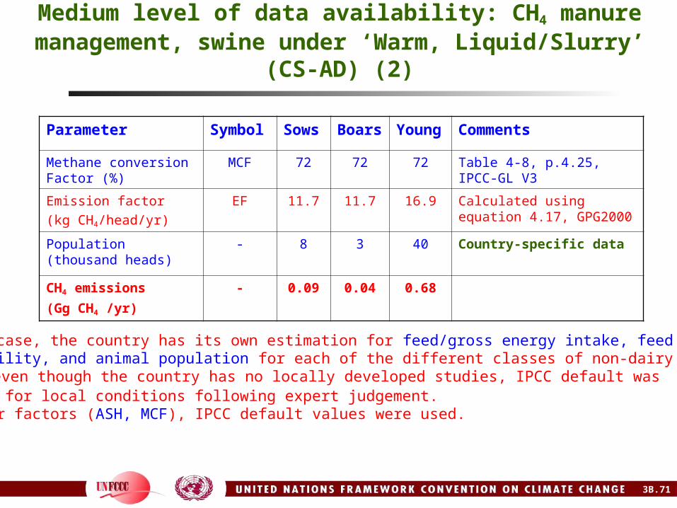
Medium level of data availability: CH4 manure management, swine under ‘Warm, Liquid/Slurry’ (CS-AD) (2)
Parameter Symbol Sows Boars Young Comments
Methane conversion Factor (%)
MCF 72 72 72 Table 4-8, p.4.25, IPCC-GL V3
Emission factor
(kg CH4/head/yr)
EF 11.7 11.7 16.9 Calculated using equation 4.17, GPG2000
Population (thousand heads)
- 8 3 40 Country-specific data
CH4 emissions
(Gg CH4 /yr)
- 0.09 0.04 0.68
In this case, the country has its own estimation for feed/gross energy intake, feeddigestibility, and animal population for each of the different classes of non-dairy cattle.For Bo, even though the country has no locally developed studies, IPCC default wasadjusted for local conditions following expert judgement.For other factors (ASH, MCF), IPCC default values were used.
3B.71

Medium level of data availability: EFs estimated by
tier 2 for non-dairy cattle, with CS AD
Climate region
Production system
EF (kg CH4/head/yr)
Cows Steers Young
Warm Extensive grazing
1.7 1.8 1.2
Intensive grazing 1.1 1.2 1.2
Feedlot 28.8 34.2 36.6
Temperate Extensive grazing
1.2 1.3 0.9
Intensive grazing 0.7 0.8 0.8
Feedlot 23.2 27.6 29.6
Weighted EF: 3.2 kg CH4/head/yrUse this value in IPCC Software
3B.72

Medium level of data availability: swine, EF estimated by tier 2, with CS AD
Climate region
Manure management
system
EF (kg CH4/head/yr)
Sows Boars Young
Warm Pasture/range/paddock
0.3 0.3 0.5
Liquid/slurry 11.7 11.7 16.8
Anaerobic lagoon 14.3 14.3 21.5
Temperate Pasture/range/paddock
0.3 0.3 0.4
Liquid/slurry 7.3 7.3 10.6
Anaerobic lagoon 14.3 14.3 21.5
Weighted EF: 1.9 kg CH4/head/yrUse this value in IPCC Software
3B.73

Medium level of data availability: results
MODULE AGRICULTURE
SUBMODULE METHANE AND NITROUS OXIDE EMISSIONS FROM DOMESTIC LIVESTOCKENTERIC FERMENTATION AND MANURE MANAGEMENT
WORKSHEET 4-1
SHEET 1 OF 2 METHANE EMISSIONS FROM DOMESTIC LIVESTOCK ENTERIC FERMENTATION AND MANURE MANAGEMENT
COUNTRY Hypothetical
YEAR 2003
STEP 1 STEP 2 STEP 3A B C D E F
Livestock Type Number of Animals
Emissions Factor for
Enteric Fermentation
Emissions from Enteric Fermentation
Emissions Factor for Manure
Management
Emissions from Manure
Management
Total Annual Emissions from
Domestic Livestock
(1000s) (kg/head/yr) (t/yr) (kg/head/yr) (t/yr) (Gg)C = (A x B) E = (A x D) F =(C + E)/1000
Dairy Cattle 1000 57 57,000.00 1.6 1,600.00 58.60
Non-dairy Cattle 5153 57 293,721.00 3.2 16,489.60 310.21
Buffalo 0 55 0.00 1.6 0.00 0.00
Sheep 3000 5 15,000.00 0.196 588.00 15.59
Goats 50 5 250.00 0.2 10.00 0.26
Camels 0 46 0.00 2.32 0.00 0.00
Horses 10 18 180.00 1.96 19.60 0.20
Mules & Asses 0 10 0.00 1.08 0.00 0.00
Swine 1505 1.5 2,257.50 1.9 2,859.50 5.12
Poultry 4000 0 0.00 0.021 84.00 0.08
Totals 368,408.50 21,650.70 390.06
Worksheet 4-1s1
Weighted EF
3B.74
3B.75
Manure Management:N2O Emissions

3B.76
Manure management – N2O
Only tier 1 provided for this source. Steps: characterization of livestock population determination of average N excretion rate for each defined
livestock category determination of fraction of N excretion that is managed in
each MMS identified determination of an EF for each MMS multiplication of total N excretion by EF, and summation of all
estimates We will continue with the assumption of a hypothetical
country in Latin America, with same animal characterization used for CH4 from manure management (and also for enteric fermentation)
One numerical example, developed here

3B.77
Livestock characterization to estimate N2O emissions from manure management
Assume that only a small fraction of the manure produced in the country undergoes some form of management
Dairy and non-dairy cattle: mostly grazing, with urine/faeces deposited directly on soil (N2O emissions accounted under “Agricultural Soils”)
Cattle in feedlots assumed to have liquid/slurry (50%) and anaerobic lagoon (50%) management systems
Swine: a small fraction as liquid/sslurry or anaerobic lagoons (Table 4.22 IPCC-GL V3)
Poultry: all manure managed (60% with / 40% without bedding) (Table 4.13 GPG2000)

Livestock characterization to estimate N2O emissions from manure management
Livestock Climate AWMSPopulation
(1000s)Fraction of
Total Pop.(%)Dairy cattle Warm Liquid/slurry 60 6.0
Anaerobic lagoon 60 6.0
Temperate Liquid/slurry 40 4.0
Anaerobic lagoon 40 4.0
Non-dairy cattle
Warm Liquid/slurry 114 2.2
Anaerobic lagoon 114 2.2
Temperate Liquid/slurry 39 0.8
Anaerobic lagoon 39 0.8
Swine Warm Liquid/slurry 51 3.4
Anaerobic lagoon 13 0.9
Temperate Liquid/slurry 30 2.0
Anaerobic lagoon 49 3.3
Poultry All With bedding 1 600 40
Without bedding 2 400 60
In case the country does not have this information, IPCC-GL provides defaultAD for different animal waste management systems (AWMS) in different regions(Table 4-21 V3).
3B.78

3B.79
Determination of average N excretion per head for identified livestock categories
IPCC-GL (Table 4-20, V3) and GPG2000 (Table 4.14) provide default values for Nex(T) for different livestock species. Use of country-specific values is recommended
County specific values can be obtained from scientific literature or industry sources, or be calculated from N intake and N retention data according to equation 4.19 (GPG2000)
Assume the country decides to use country-specific values to estimate Nex(T) for non-dairy cattle only, and that default values are used for all other categories

3B.80
Determination of country-specific average N excretion per head for non-dairy cattle
Assume that the country has information about crude protein content of feed for the different classes identified
Crude protein data are combined with feed intake data (from the same livestock characterization used for estimating CH4 emissions) to obtain N intake
Assume that the country uses IPCC default value for N retention in body and products (0.07 for non-dairy cattle, GPG2000, Table 4.15)

Livestock characterization for estimating N2O emissions from manure management
Climate
region
MMS* Livestock
category
Pop.
(1000s)
Feed intake
(kg/day)
Crude protein
(%)
N intake (kg/head/yr)
N retention
N excretion (kg/head/yr)
Warm L/S Cows 20 5.7 15 50 0.07 47
Steers 46 6.8 15 60 0.07 55
Young 48 7.3 15 64 0.07 59
AL Cows 20 5.7 15 50 0.07 47
Steers 46 6.8 15 60 0.07 55
Young 48 7.3 15 64 0.07 59
Temp L/S Cows 7 5.7 16 53 0.07 50
Steers 16 6.8 16 63 0.07 59
Young 16 7.3 16 68 0.07 63
AL Cows 7 5.7 16 53 0.07 50
Steers 16 6.8 16 63 0.07 59
Young 16 7.3 16 68 0.07 63
* MMS = Manure management system L/S = Liquid/slurry AL = Anaerobic lagoon
3B.81

3B.82
Determination of average N excretion per head for non-dairy cattle
Values estimated for Nex(T), using a combination of country-specific and default data, ranged between 47 and 63 kg N/head/yr for a population of non-dairy cattle in feedlots, with a weighted average of 56 kg N/head/yr. This value should be introduced in IPCC software
This value is higher than the IPCC default for Latin America (40 kg N/head/yr), which is based on grazing cattle
Default values were used for the other species

N2O from manure management: use of IPCC software to estimate total N excretion (1)
MODULE AGRICULTURE
SUBMODULE METHANE AND NITROUS OXIDE EMISSIONS FROM DOMESTIC LIVESTOCK ENTERIC FERMENTATION AND MANURE MANAGEMENT
WORKSHEET 4-1 (SUPPLEMENTAL)
SPECIFY AWMS ANAEROBIC LAGOONS
SHEET NITROGEN EXCRETION FOR ANIMAL WASTE MANAGEMENT SYSTEM
COUNTRY Hypothetical
YEAR 2003
A B C DLivestock Type Number of Animals Nitrogen Excretion
NexFraction of Manure
Nitrogen per AWMS (%/100)
Nitrogen Excretion per AWMS, Nex
(# of animals) (kg//head/(yr) (fraction) (kg/N/yr)D = (A x B x C)
Non-dairy Cattle 5153000 56 0.03 8,657,040.00
Dairy Cattle 1000000 70 0.1 7,000,000.00
Poultry 4000000 0 0.00
Sheep 3000000 0 0.00
Swine 1500000 16 0.042 1,008,000.00
Others 0.00
TOTAL 16,665,040.00
Estimated
IPCC Default
IPCC Default
Data from livestock characterization
3B.83

MODULE AGRICULTURE
SUBMODULE METHANE AND NITROUS OXIDE EMISSIONS FROM DOMESTIC LIVESTOCK ENTERIC FERMENTATION AND MANURE MANAGEMENT
WORKSHEET 4-1 (SUPPLEMENTAL)
SPECIFY AWMS LIQUID SYSTEMS
SHEET NITROGEN EXCRETION FOR ANIMAL WASTE MANAGEMENT SYSTEM
COUNTRY Hypothetical
YEAR 2003
A B C DLivestock Type Number of Animals Nitrogen Excretion
NexFraction of Manure
Nitrogen per AWMS (%/100)
Nitrogen Excretion per AWMS, Nex
(1000s) (kg//head/(yr) (fraction) (kg/N/yr)
D = (A x B x C)
Non-dairy Cattle 5153000 56 0.03 8,657,040.00
Dairy Cattle 1000000 70 0.1 7,000,000.00
Poultry 4000000 0 0.00
Sheep 3000000 0 0.00
Swine 1500000 16 0.054 1,296,000.00
Others 0.00
TOTAL 16,953,040.00
N2O from manure management: use of IPCC software to estimate total N excretion (2)
Calculated
IPCC Default
IPCC Default
Data from livestock characterization
3B.84

MODULE AGRICULTURE
SUBMODULE METHANE AND NITROUS OXIDE EMISSIONS FROM DOMESTIC LIVESTOCK ENTERIC FERMENTATION AND MANURE MANAGEMENT
WORKSHEET 4-1 (SUPPLEMENTAL)
SPECIFY AWMS OTHER (POULTRY MANURE WITH BEDDING)
SHEET NITROGEN EXCRETION FOR ANIMAL WASTE MANAGEMENT SYSTEM
COUNTRY Hypothetical
YEAR 2003
A B C DLivestock Type Number of Animals Nitrogen Excretion
NexFraction of Manure
Nitrogen per AWMS (%/100)
Nitrogen Excretion per AWMS, Nex
(1000s) (kg//head/(yr) (fraction) (kg/N/yr)
D = (A x B x C)
Non-dairy Cattle 0.00
Dairy Cattle 0.00
Poultry 4000000 0.6 0.6 1,440,000.00
Sheep 0.00
Swine 0.00
Others 0.00
TOTAL 1,440,000.00
N2O from manure management: use of IPCC software to estimate total N excretion (3)
IPCC Default
Data from livestock characterization
3B.85

MODULE AGRICULTURE
SUBMODULE METHANE AND NITROUS OXIDE EMISSIONS FROM DOMESTIC LIVESTOCK ENTERIC FERMENTATION AND MANURE MANAGEMENT
WORKSHEET 4-1 (SUPPLEMENTAL)
SPECIFY AWMS OTHER (POULTRY MANURE WITHOUT BEDDING)
SHEET NITROGEN EXCRETION FOR ANIMAL WASTE MANAGEMENT SYSTEM
COUNTRY Hypothetical
YEAR 2003
A B C DLivestock Type Number of Animals Nitrogen Excretion
NexFraction of Manure
Nitrogen per AWMS (%/100)
Nitrogen Excretion per AWMS, Nex
(1000s) (kg//head/(yr) (fraction) (kg/N/yr)D = (A x B x C)
Non-dairy Cattle 0.00
Dairy Cattle 0.00
Poultry 4000000 0.6 0.4 960,000.00
Sheep 0.00
Swine 0.00
Others 0.00
TOTAL 960,000.00
N2O from manure management: use of IPCC software to estimate total N excretion (4)
IPCC Default
Data from livestock characterization
3B.86

MODULE AGRICULTURE
SUBMODULE METHANE AND NITROUS OXIDE EMISSIONS FROM DOMESTIC LIVESTOCK ENTERIC FERMENTATION AND MANURE MANAGEMENT
WORKSHEET 4-1
SHEET 2 OF 2 NITROUS OXIDE EMISSIONS FROM ANIMAL PRODUCTION EMISSIONS FROM ANIMAL WASTE MANAGEMENT SYSTEMS (AWMS)
COUNTRY Hypothetical
YEAR 2003
STEP 4A B C
Animal Waste Nitrogen Excretion Emission Factor For Total Annual Emissions Management System Nex(AWMS) AWMS of N2O (AWMS) EF3
(kg N/yr) (kg N2O–N/kg N) (Gg)
C=(AxB)[44/28] / 1 000 000
Anaerobic lagoons 16,665,040.00 0.001 0.03
Liquid systems 16,953,040.00 0.001 0.03
Daily spread 960,000.00
Poultry manure with bedding 1,440,000.00 0.02 0.05
Pasture range and paddock 0.00
Poultry manure w/o bedding 960,000.00 0.005 0.01
Total 36,978,080.00 Total 0.11
Use of IPCC software for estimating N2O from manure management
IPCC Default
IPCC Default
IPCC defaults obtained from Table 4-22, IPCC-GL V3, and Tables 4.12 and 4.13, GPG2000.
IPCC Default
IPCC Default
Note: cells corresponding to poultry were manually altered to accommodatethese new categories from GPG2000, not included in IPCC-GL.
3B.87
3B.88
Direct N2O Emissions from Agricultural Soils

AnthropogenicN inputs to soils
Mineral fertilizers
Histosols cultivation
N-fixing crops
Sewage sludges
Crop residues
Animal manures
Fraction of …(from the mass balance)
Other practicesdealing with soil N
3B.89

Assess individual contribution of different N sources to determineones (subcategories) which are significant for the source category(25% or more of source category N2O emissions)
For this, apply Tier 1a method and default values to get an economic emission estimate
For the significant subcategories, the best efforts should be invested to apply Tier 1b along with country-specific AD1 and AD2 (parameters) and country-specific emission factors
For non-significant subcategories, Tier 1a, along with country-specificAD1, default AD2 (parameters) and default emission factors, is acceptable
AGRICULTURAL SOILS
It is also acceptable to mix Tiers 1a and 1b for different N sources, which willdepend on the activity data availability
3B.90

3B.91
Direct N2O – Agricultural soils
Assumption of the same hypothetical country
We will assume that the country has the following AD: usage of synthetic N fertilizers (FAO database) usage of synthetic N fertilizers for barley crop (industry source) estimate of EF1 for N applied to barley crops (local research), which
due to improved practices in this crop (e.g. fractioning of N applications), is lower than the IPCC default EF
N excretion from different animal categories under pasture/range/paddock AWMS (data from previous example of N2O from manure management)
area devoted to N-fixing crops (FAO database)
The country has no organic soils (histosols)
Direct N2O emissions are estimated using a combination of Tier 1a (for most of the sources) and Tier 1b (for use of N fertilizers in barley crop and N in crop residues)

Use of N fertilizers
From the FAO database:
Crop Area
(1000 ha)
Crop yield
(kg/ha)
Use of N fertilizer
(1000 t N)
Wheat 824 1 545 n/a
Barley 1 356 (371) 1 488 (1400) 19.1
Maize 1 225 2 233 n/a
Rice 98 4 800 n/a
Soybeans 231 1 982 n/a
Potatoes 25 18 000 n/a
Total 2 779 -- 130
1 Barley data from industry sources, shown in parentheses.
3B.92

3B.93
Direct N2O – Agricultural soils
From FAO database, only total country data for fertilizer use are available. Therefore, only Tier 1a method could be used
Data from barley industry/research can be used to apply Tier 1b method: to ensure consistency, it is recommended to compare crop area and crop yield
data from FAO with data from local industry in this case, the two sources reasonably matched in terms of area and yield, and it
can be assumed that the industry estimation of N fertilizer usage is compatible with the FAO N fertilizer data
from previous table, it can be derived that 19,000 t N fertilizer were applied to barley crops, and 111,000 t N fertilizer to the rest (130,000 minus 19,000)
from local research, EF1 was estimated to be 0.9% for fertilizer applied to barley crops in the country
Since there are no organic soils in the country, EF2 is not needed Emissions from grazing livestock are included here. Note that the GPG2000
includes this source under manure management

3B.94
Synthetic fertilizers:determination of FSN and EF1
FSN: annual amount of fertilizer N applied to soils, adjusted by amount of N that volatilizes as NH3 and NOx
To adjust for volatilization, use IPCC default value from Table 4-17, IPCC-GL, V2: 0.1 kg (NOx+NH3)-N/kg fertilizer-N
It is determined that: FSN = 19,000 (1-0.1) = 17,100 t fertilizer-N (barley) FSN = 111,000 (1-0.1) = 99,900 t fertilizer-N (all other
crops) Total fertilizer-N = 117,000 t fertilizer-N
EF1 is 0.9% for barley (country specific) and 1.25% for the other crops (Table 4.17, GPG2000)
For the purpose of filling the IPCC software sheet 4-5s1, a weighted EF1 is calculated as follows:
EF1 = weighted average = 17.1/117 (0.9) + 99.9/117 (1.25) = 1.20% From worksheet 4-5s1, the annual emission of N2O-N from use of synthetic fertilizer
was estimated as 1.40 Gg N2O-N
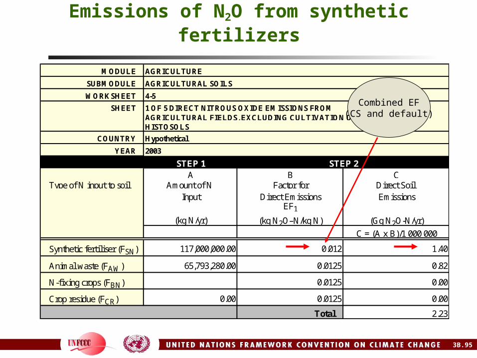
Emissions of N2O from synthetic fertilizers
MODULE AGRICULTURE
SUBMODULE AGRICULTURAL SOILS
WORKSHEET 4-5
SHEET 1 OF 5 DIRECT NITROUS OXIDE EMISSIONS FROM AGRICULTURAL FIELDS, EXCLUDING CULTIVATION OFHISTOSOLS
COUNTRY Hypothetical
YEAR 2003
STEP 1 STEP 2A B C
Type of N input to soil Amount of N Factor for Direct Soil Input Direct Emissions Emissions
EF1
(kg N/yr) (kg N2O–N/kg N) (Gg N2O-N/yr)
C = (A x B)/1 000 000
Synthetic fertiliser (FSN) 117,000,000.00 0.012 1.40
Animal waste (FAW) 65,793,280.00 0.0125 0.82
N-fixing crops (FBN) 0.0125 0.00
Crop residue (FCR) 0.00 0.0125 0.00
Total 2.23
Combined EF(CS and default)
3B.95

3B.96
Manure applied to soils:determination of FAM
FAM: annual amount of manure N applied to soils, adjusted by amount of N that volatilizes as NH3 and NOx
To calculate amount of manure N applied to soils, use total amount of manure produced (using livestock characterization previously applied to other sources) and subtract the amounts used for fuel, feed and construction (here assumed to be zero) and those deposited on soils by grazing livestock (whose emissions are reported separately as direct emissions)
To adjust for volatilization, use IPCC default value from Table 4-17, IPCC-GL, V2: 0.2 kg (NOx+NH3)-N/kg animal manure N
It is determined that: FAM = 24,924 t animal manure N applied to soils
Next two slides illustrate the use of IPCC software to estimate FAM (named as FAW in IPCC-GL) and estimation of an annual emission of N2O-N from application of animal manure to soil of 0.31 Gg N2O-N

Emissions of N2O from animal manure (1)
Country’s estimate
From Table 4-17IPCC Guidelines V2
MODULE AGRICULTURE
SUBMODULE AGRICULTURAL SOILS
WORKSHEET 4-5A (SUPPLEMENTAL)
SHEET 1 OF 1 MANURE NITROGEN USED
COUNTRY Hypothetical
YEAR 2003
A B C D E FTotal Nitrogen Fraction of Nitrogen Fraction of Nitrogen Fraction of Nitrogen Sum Manure Nitrogen Used
Excretion Burned for Fuel Excreted During Excreted Emitted as (corrected for NOX and Grazing NOX and NH3 NH3 emissions), FAW
(kg N/yr) (fraction) (fraction) (fraction) (fraction) (kg N/yr)
F = 1 - (B + C + D) F = (A x E)
249,240,080.00 0 0.7 0.2 0.10 24,924,008.00
Data from livestockcharacterization
3B.97

MODULE AGRICULTURE
SUBMODULE AGRICULTURAL SOILS
WORKSHEET 4-5
SHEET 1 OF 5 DIRECT NITROUS OXIDE EMISSIONS FROM AGRICULTURAL FIELDS, EXCLUDING CULTIVATION OFHISTOSOLS
COUNTRY Hypothetical
YEAR 2003
STEP 1 STEP 2A B C
Type of N input to soil Amount of N Factor for Direct Soil Input Direct Emissions Emissions
EF1
(kg N/yr) (kg N2O–N/kg N) (Gg N2O-N/yr)
C = (A x B)/1 000 000
Synthetic fertiliser (FSN) 117,000,000.00 0.012 1.40
Animal waste (FAW) 24,924,008.00 0.0125 0.31
N-fixing crops (FBN) 0.0125 0.00
Crop residue (FCR) 0.0125 0.00
Total 1.72
Emissions of N2O from animal manure (2)
IPCC default
3B.98

3B.99
N-fixing crops:determination of FBN
FBN: amount of N fixed by N-fixing crops cultivated annually (in our case, soybeans)
To calculate amount of N fixed, we assume that there are no crop-specific values for grain/biomass ratio or for moisture content of biomass; therefore, default data are used
Grain production is estimated from FAO statistics (457,842 t/yr) N content of biomass (FracNCRBF) is obtained from Table 4.16 (GPG2000):
0.023 kg N/kg dry biomass Residue/crop product ratio is 2:1, and dry matter fraction is 0.85 (from
same table as above) It is determined (by using equation 4.26, GPG2000) that:
FBN= 27,748 t fixed-N This value is introduced in IPCC software worksheet 4-4s1 to estimate an
annual emission of N2O-N from N-fixing crops of 0.35 Gg N2O-N

MODULE AGRICULTURE
SUBMODULE AGRICULTURAL SOILS
WORKSHEET 4-5
SHEET 1 OF 5 DIRECT NITROUS OXIDE EMISSIONS FROM AGRICULTURAL FIELDS, EXCLUDING CULTIVATION OFHISTOSOLS
COUNTRY Hypothetical
YEAR 2003
STEP 1 STEP 2A B C
Type of N input to soil Amount of N Factor for Direct Soil Input Direct Emissions Emissions
EF1
(kg N/yr) (kg N2O–N/kg N) (Gg N2O-N/yr)
C = (A x B)/1 000 000
Synthetic fertiliser (FSN) 117,000,000.00 0.012 1.40
Animal waste (FAW) 24,924,008.00 0.0125 0.31
N-fixing crops (FBN) 27748000 0.0125 0.35
Crop residue (FCR) 0.0125 0.00
Total 2.06
Emissions of N2O from N-fixing crops
IPCC defaultEstimatedactivity data
3B.100

3B.101
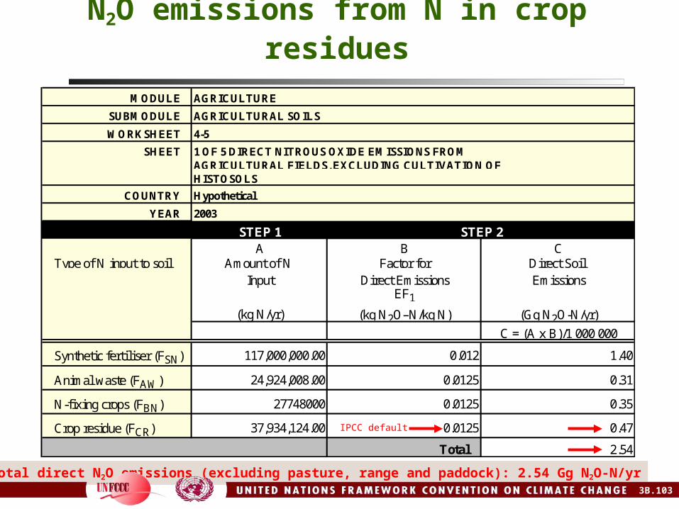
Crop residues:determination of FCR
FCR: amount of N in crop residues returned to soil annually It is estimated by adjusting the total amount of crop residue N produced
to account for the fraction that is burned in the field and for the fraction that is removed from the field
We assume that the country has enough data to apply Tier 1b method (equation 4.29 in GPG2000)
It is determined that:
FCR = 37,934 t N in crop residues that are returned to soils
This value is introduced in sheet 4-5s1 of the IPCC software to estimate an annual emission of N2O-N from N in crop residues of 0.47 Gg N2O-N
IPCC Software worksheet was designed for Tier-1a method, and use of Tier 1b requires manually altering sheet 4-5s1, cell C23

Crop residues: determination of FCR
Crop Crop (1000 t)
(1)
Res/Crop
(2)
FracDM
(2)
FracNCR
(2)
FracBURN
(3)
FracFUEL
(3)
FracFOD
(3)
Eq. 4.29 GPG
(t N20-N)
Wheat 1,273 1.3 0.85 0.0028 0.2 0 0.1 2,757
Barley 148 1.2 0.85 0.0043 0.2 0 0.1 456
Maize 2,735 1.0 0.78 0.0081 0 0.2 0.2 10,369
Rice 470 1.4 0.90 0.0067 0 0 0 3,971
Soybean 458 2.1 0.85 0.023 0 0 0 18,797
Potatoes 450 0.4 0.80 0.011 0 0 0 1,584
Total --- --- --- --- --- --- --- 37,934
(1) Source: FAO statistics(2) Source: Table 4.16, GPG2000 (except FracDM for potatoes, which was estimated by experts)(3) Source: Country-specific data FCR
3B.102
MODULE AGRICULTURE
SUBMODULE AGRICULTURAL SOILS
WORKSHEET 4-5
SHEET 1 OF 5 DIRECT NITROUS OXIDE EMISSIONS FROM AGRICULTURAL FIELDS, EXCLUDING CULTIVATION OFHISTOSOLS
COUNTRY Hypothetical
YEAR 2003
STEP 1 STEP 2A B C
Type of N input to soil Amount of N Factor for Direct Soil Input Direct Emissions Emissions
EF1
(kg N/yr) (kg N2O–N/kg N) (Gg N2O-N/yr)
C = (A x B)/1 000 000
Synthetic fertiliser (FSN) 117,000,000.00 0.012 1.40
Animal waste (FAW) 24,924,008.00 0.0125 0.31
N-fixing crops (FBN) 27748000 0.0125 0.35
Crop residue (FCR) 37,934,124.00 0.0125 0.47
Total 2.54
N2O emissions from N in crop residues
Total direct N2O emissions (excluding pasture, range and paddock): 2.54 Gg N2O-N/yr
IPCC default
3B.103

MODULE AGRICULTURE
SUBMODULE METHANE AND NITROUS OXIDE EMISSIONS FROM DOMESTIC LIVESTOCK ENTERIC FERMENTATION AND MANURE MANAGEMENT
WORKSHEET 4-1 (SUPPLEMENTAL)
SPECIFY AWMS PASTURE RANGE AND PADDOCK
SHEET NITROGEN EXCRETION FOR ANIMAL WASTE MANAGEMENT SYSTEM
COUNTRY Hypothetical
YEAR 2003
A B C DLivestock Type Number of Animals Nitrogen Excretion
NexFraction of Manure
Nitrogen per AWMS (%/100)
Nitrogen Excretion per AWMS, Nex
(1000s) (kg//head/(yr) (fraction) (kg/N/yr)D = (A x B x C)
Non-dairy Cattle 5153000 40 0.95 195,814,000.00
Dairy Cattle 1000000 70 0.2 14,000,000.00
Poultry 4000000 0.00
Sheep 3000000 0.00
Swine 1500000 16 0.102 2,448,000.00
Others 0.00
TOTAL 212,262,000.00
N excretion from pasture/range/paddock
Default values3B.104

N2O emissions from pasture/range/paddock
MODULE AGRICULTURE
SUBMODULE AGRICULTURAL SOILS
WORKSHEET 4-5
SHEET 3 OF 5 NITROUS OXIDE SOIL EMISSIONS FROM GRAZING ANIMALS - PASTURE RANGE AND PADDOCK
COUNTRY Hypothetical
YEAR 2003
STEP 5A B C
Animal Waste Nitrogen Excretion Emission Factor for Emissions Of N2O from
Management System Nex(AWMS) AWMS Grazing Animals
(AWMS) EF3 (kg N/yr) (kg N2O–N/kg N) (Gg)
C = (A x B)[44/28]/1 000 000
Pasture range & paddock 212,262,000.00 0.02 6.67
From Table 4-8IPCC Guidelines V2
3B.105

3B.106
Indirect N2O Emissions from Agricultural Soils

3B.107
Indirect N2O – Agricultural soils
We will continue with the assumption of a hypothetical country in Latin America
We will assume that the country only covers the following sources: N2O(G): from volatilization of applied synthetic fertilizer and animal
manure N, and its subsequent deposition as NOx and NH4
N2O(L): from leaching and runoff of applied fertilizer and animal manure
Indirect N2O emissions are estimated using Tier 1a method and IPCC default emission factors
The next slides show calculations as performed by IPCC Software

Indirect N2O emissions from atmospheric depositions
MODULE AGRICULTURE
SUBMODULE AGRICULTURAL SOILS
WORKSHEET 4-5
SHEET 4 OF 5 INDIRECT NITROUS OXIDE EMISSIONS FROM ATMOSPHERIC DEPOSITION OF NH3 AND NOXCOUNTRY Hypothetical
YEAR 2003
STEP 6A B C D E F G H
Type of Synthetic Fraction of Amount of Total N Fraction of Total N Excretion Emission Factor Nitrous Oxide Deposition Fertiliser N Synthetic Synthetic N Excretion by Total Manure N by Livestock that EF4
Emissions
Applied to Fertiliser N Applied to Soil Livestock Excreted that Volatilizes Soil, NFERT
Applied that that Volatilizes NEX Volatilizes
Volatilizes FracGASMFracGASFS
(kg N/yr) (kg N/kg N) (kg N/kg N) (kg N/yr) (kg N/kg N) (kg N/kg N) (kg N2O–N/kg N) (Gg N2O–N/yr)
C = (A x B) F = (D x E) H = (C + F) x G /1 000 000
Total 130000000 0.1 13,000,000.00 249,240,080.00 0.2 49,848,016.00 0.01 0.63
From Table 4-17IPCC Guidelines V2
From Table 4.18GPG2000
Default value
3B.108

MODULE AGRICULTURE
SUBMODULE AGRICULTURAL SOILS
WORKSHEET 4-5
SHEET 5 OF 5 INDIRECT NITROUS OXIDE EMISSIONS FROM LEACHING
COUNTRY Hypothetical
YEAR 2003
STEP 7 STEP 8I J K L M N
Synthetic Fertiliser Livestock N Fraction of N That Emission Factor Nitrous Oxide Emissions Total Indirect Use NFERT Excretion NEX Leaches EF5
From Leaching Nitrous Oxide
FracLEACH Emissions
(kg N/yr) (kg N/yr) (kg N/kg N) (Gg N2O–N/yr) (Gg N2O/yr)
M = (I + J) x K x L/1 000 000 N = (H + M)[44/28]
130,000,000.00 249,240,080.00 0.3 0.025 2.84 5.46
Indirect N2O emissions from leaching and runoff
From Table 4-17IPCC Guidelines V2
From Table 4.18GPG2000
3B.109
3B.110
Field Burning of Crop Residues

3B.111
• If not occurring, then emission estimates are “NO”• If occurring, then emissions must be estimated using
worksheet 4-4 sheets 1-2-3 (IPCC software)• Only one method is available to estimate emissions from
this source category• If key source, then country-specific values for non-
collectable AD and emission factors must preferrably be used (default values for key sources are possible if the country cannot provide the required AD or financial resources are lacking)
• If country-specific values are used, they must be reported in a transparent manner
Burning of crop residuesMain issues derived from the decision tree

3B.112
• Activity data required to estimate emissions:• collected by statistics agencies: annual crop
production (alternate way is FAO database)• not collected by statistics agencies:
• residue to crop ratio• dry matter fraction of biomass• fraction of crop residues burned in field• fraction of crop residues oxidized• C fraction in dry matter• Nitrogen/carbon ratio
• Emission factors: C-N emission ratios as CH4, CO, N2O, NOX
• Other constants (conversion ratios):• C to CH4 or CO (16/12; 28/12, respectively)• N to N2O or NOX (44/28; 46/14, respectively)
Burning of crop residues

3B.113
MODULE AGRICULTURE
SUBMODUL
E FIELD BURNING OF AGRICULTURAL RESIDUES
WORKSHEE
T 4-4
SHEET 1 OF 3
COUNTRY FICTICIOUS LAND
YEAR 2002
STEP 1 STEP 2 STEP 3
Crops A B C D E F G H
(specify locally Annual Residue to Quantity of Dry Matter Quantity of Fraction Fraction Total Biomass
important Production Crop Ratio Residue Fraction Dry Residue Burned in Oxidised Burned
crops) Fields
(Gg crop) (Gg biomass) (Gg dm) (Gg dm)
C = (A x B) E = (C x D) H = (E x F xG)
0,00 0,00 0,00
Wheat 15750 1,3 20.475,00 0,85 17.403,75 0,75 0,9 11.747,53
Maize 5200 1 5.200,00 0,5 2.600,00 0,5 0,9 1.170,00
Rice 1050 1,4 1.470,00 0,85 1.249,50 0,85 0,9 955,87
. 0,00 0,00 0,00
1. OPEN THE IPCC SOFTWARE AND CHOOSE THE YEAR OF THE INVENTORY2. CLICK 0N “SECTORS” IN THE MENU BAR, AND THEN CLICK ON AGRICULTURE3. OPEN SHEET 4-4s2
Main residue-producing crops:Cereals (wheat, barley, oats, rye, rice,maize, sorghum)SugarcanePulses (peas, beans, lentils)Potatoes, peanut, others
Identify theexisting residue-producing crops
3B.114
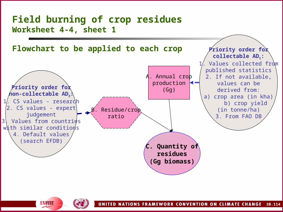
B. Residue/cropratio
A. Annual cropproduction
(Gg)
C. Quantity ofresidues
(Gg biomass)
Field burning of crop residuesWorksheet 4-4, sheet 1
Flowchart to be applied to each crop Priority order forcollectable AD1:
1. Values collected frompublished statistics2. If not available,
values can bederived from:
a) crop area (in kha)b) crop yield
(in tonne/ha)3. From FAO DB
Priority order fornon-collectable AD2:1. CS values - research2. CS values - expert
judgement3. Values from countrieswith similar conditions
4. Default values(search EFDB)

3B.115
D. Dry matterFraction
E. Total quantity ofdry residue
(Gg dm)
C. Quantity ofresidue
(Gg biomass)from previous slide
Priority order fornon-collectable AD:1. CS values - research2. CS values - expert
judgement3. Values from countrieswith similar conditions4. IPCC default values
(search EFDB)
Field burning of crop residuesWorksheet 4-4, sheet 1
Flowchart to be applied to each crop

3B.116
E. Quantity ofdry residue
(Gg dm)from previous slide
F. Fraction burnedin fields
H. Total biomassburned
(Gg dm burned)
G. Fractionoxidized
Priority order fornon-collectable AD:1. CS values - research2. CS values - expert
judgement3. Values from countrieswith similar conditions
(no default values)
For default values,search EFDB as
combustion efficiency
To avoid doublecounting, a mass balance
of crop residue biomass mustbe internally performed:Fburned= Total biomass –(Fremoved from the field+
Featen by animals+Fother uses)
Field burning of crop residuesWorksheet 4-4, sheet 1
Flowchart to be applied to each crop

4. OPEN SHEET 4-4s2 OF “AGRICULTURE” UNDER “SECTORS”
MODULE AGRICULTURE
SUBMODULE FIELD BURNING OF AGRICULTURAL RESIDUES
WORKSHEET 4-4
SHEET 2 OF 3
COUNTRY FICTICIOUS LAND
YEAR 2002
STEP 4 STEP 5
I J K L
Carbon Total Carbon Nitrogen- Total Nitrogen
Fraction of Released Carbon Ratio Released
Crops Residue
(Gg C) (Gg N)
J = (H x I) L = (J x K)
0,00 0,00
Wheat 0,48 5.638,82 0,012 67,67
Maize 0,47 549,90 0,02 11,00
Rice 0,41 391,91 0,014 5,49
. 0,00 0,00
3B.117

3B.118
H. Biomass burned(Gg dm burned)
from previous slideI. C fractionin residue
J. C released(Gg C)
Priority order fornon-collectable AD:1. CS values - research2. CS values - expert
judgement3. Values from countrieswith similar conditions
4. Default values(search EFDB)
K. N/C ratio
L. N released(Gg N)
Total C and N releasedare obtained by
addding the valuesobtained per each
individual crop
Field burning of crop residuesWorksheet 4-4, sheet 2
Flowchart to be applied to each crop

Worksheet 4-4, sheet 3
5. OPEN SHEET 4-4s3 OF “AGRICULTURE” UNDER “SECTORS”
MODULE AGRICULTURE
SUBMODULE FIELD BURNING OF AGRICULTURAL RESIDUES
WORKSHEET 4-4
SHEET 3 OF 3
COUNTRY FICTICIOUS LAND
YEAR 2002
STEP 6
M N O P
Emission Ratio Emissions Conversion Ratio Emissions
from Field
Burning of
Agricultural
Residues
(Gg C or Gg N) (Gg)
N = (J x M) P = (N x O)
CH4 0,005 32,90 16/12 43,87
CO 0,06 394,84 28/12 921,29
N = (L x M) P = (N x O)
N2O 0,007 0,59 44/28 0,93
NOx 0,121 10,18 46/14 33,46
Total emissionestimates
3B.119

6. GO TO THE “OVERVIEW” MODULE7. OPEN THE WORHSHEET 4-S2TABLE 4 SECTORAL REPORT FOR AGRICULTURE
(Sheet 2 of 2)
SECTORAL REPORT FOR NATIONAL GREENHOUSE GAS INVENTORIES
(Gg)
GREENHOUSE GAS SOURCE AND SINK CATEGORIES CH4 N2O NOx CO NMVOC
B Manure Management (cont...)
10 Anaerobic 0
11 Liquid Systems 0
12 Solid Storage and Dry Lot 0
13 Other (please specify) 0
C Rice Cultivation 0
1 Irrigated 0
2 Rainfed 0
3 Deep Water 0
4 Other (please specify)
D Agricultural Soils 0
E Prescribed Burning of Savannas 1 0 2 36
F Field Burning of Agricultural Residues (1) 44 1 33 921
1 Cereals
2 Pulse
3 Tuber and Root
4 Sugar Cane
5 Other (please specify)
G Other (please specify)
Total emissionestimates
3B.120

Total C released(Gg C from all crops)from previous slide
Total N released(Gg N from all crops)from previous slide
MNon-CO2
emission rates(search EFDB)
OConversion
ratios
C-Nemitted
(Gg C emitted asCH4 or CO;
Gg N emitted asN2O or NOX)
PCH4 emitted
(Gg CH4)
PCO emitted
(Gg CO)
PN2O emitted
(Gg N2O)
PNOX emitted
(Gg NOX)
EFs:If no CS values,
use defaults(Table 4-16, Reference Manual,
Rev. 1996 IPCC Guidelines)
Field burning of crop residuesWorksheet 4-4, sheet 3
Flowchart to be applied to aggregated figures
3B.121

Field burning of crop residues
Emission factors
3B.122

Field burning of crop residuesEmission estimates using country-specific values
Wheat residues (1 of 3)
MODULE AGRICULTURE
SUBMODUL
E FIELD BURNING OF AGRICULTURAL RESIDUES
WORKSHEE
T 4-4
SHEET 1 OF 3
COUNTRY FICTICIOUS
YEAR 2002
STEP 1 STEP 2 STEP 3
Crops A B C D E F G H
(specify locally
Annual Residue to Quantity of Dry
Matter Quantity of Fraction Fraction
Total Biomass
important Production Crop Ratio Residue FractionDry
ResidueBurned in Oxidised Burned
crops) Fields
(Gg crop) (Gg biomass) (Gg dm) (Gg dm)
C = (A x B) E = (C x D) H = (E x F
xG)
Wheat 18.350,50 1,50 27.525,8 0,90 24.773,2 0,12 0,96 2.735,0
AD fromnational statistics
CS activity data,from research and
monitoring
3B.123

3B.124
Field burning of crop residues Emission estimates using country-specific values
Wheat residues (2 of 3)
MODULE AGRICULTURE
SUBMODULE FIELD BURNING OF AGRICULTURAL RESIDUES
WORKSHEET 4-4
SHEET 2 OF 3
COUNTRY FICTICIOUS
YEAR 2002
STEP 4 STEP 5
I J K L
Carbon Total Carbon Nitrogen- Total Nitrogen
Fraction of Released Carbon Ratio Released
Crops Residue
(Gg C) (Gg N)
J = (H x I) L = (J x K)
Wheat 0,45 1.230,7 0,0032 3,94
CS activity data,from research and
monitoring

3B.125
Field burning of crop residues Emission estimates using country-specific values
Wheat residues (3 of 3)
MODULE AGRICULTURE
SUBMODULE FIELD BURNING OF AGRICULTURAL RESIDUES
WORKSHEET 4-4
SHEET 3 OF 3
COUNTRY FICTICIOUS
YEAR 2002
STEP 6
M N O P
Gas Emission Ratio Emissions Conversion Ratio Emissions
(Gg C or Gg N) (Gg)
N = (J x M) P = (N x O)
CH4 0,00311 3,83 16/12 5,10
CO 0,06 73,84 28/12 172,30
N = (L x M) P = (N x O)
N2O 0,018 0,07 44/28 0,11
NOx 0,121 0,48 46/14 1,57
CS values for CH4/N2OD for CO/NOX

Field burning of crop residues Emission estimates using default values
Wheat residues (1 of 3) MODULE AGRICULTURE
SUBMODULE FIELD BURNING OF AGRICULTURAL RESIDUES
WORKSHEET 4-4
SHEET 1 OF 3
COUNTRY FICTICIOUS
YEAR 2002
STEP 1 STEP 2 STEP 3
Crops A B C D E F G H
(specify locally
Annual Residue toQuantity
of Dry Matter
Quantity of
Fraction Fraction Total
Biomass
important Production Crop Ratio Residue FractionDry
ResidueBurned
in Oxidised Burned
crops) Fields
(Gg crop) (Gg biomass)
(Gg dm) (Gg dm)
EF ID= 43555
C = (A x B)
EF ID= 43636
E = (C x D)
EF ID= 45941
H = (E x F xG)
Wheat 18.350,5 1,30 23.855,7 0,83 19.800,2 0,12 0,94 2.140,4
CS value,from monitoring orexpert judgement
AD:1. from
national statistics, or2. from FAO database:
(www.fao.org, then “FAOSTAT-Agriculture” and “Crops primary”)
Activity data,taken from EFDB
3B.126

3B.127
Field burning of crop residuesEmission estimates using default values
Wheat residues (2 of 3)
Default activity data,from EFDB
MODULE AGRICULTURE
SUBMODULE FIELD BURNING OF AGRICULTURAL RESIDUES
WORKSHEET 4-4
SHEET 2 OF 3
COUNTRY FICTICIOUS
YEAR 2002
STEP 4 STEP 5
I J K L
Carbon Total Carbon Nitrogen- Total Nitrogen
Fraction of Released Carbon Ratio Released
Crops Residue
(Gg C) (Gg N)
J = (H x I) L = (J x K)
Wheat 0,48 1.027,4 0,012 12,33
EF ID= 43716 EF ID= 43796

3B.128
Field burning of crop residuesEmission estimates using CS values
Wheat residues (3 of 3)
Default values,from EFDB
MODULE AGRICULTURE
SUBMODULE FIELD BURNING OF AGRICULTURAL RESIDUES
WORKSHEET 4-4
SHEET 3 OF 3
COUNTRY FICTICIOUS
YEAR 2002
STEP 6
M N O P
Emission Ratio Emissions Conversion Ratio Emissions
(Gg C or Gg N) (Gg)
N = (J x M) P = (N x O)
CH4 0,005 5,14 16/12 6,85
CO 0,06 61,64 28/12 143,83
N = (L x M) P = (N x O)
N2O 0,007 0,09 44/28 0,14
NOx 0,121 1,49 46/14 4,90
EF ID=43583, 43548, 43543, 43549

3B.129
Field burning of crop residues Differences in emission estimates
if country-specific or default values are used
Emissions Emissions Per cent
Gas emitted Gg gas Gg gas of
using using difference
CS values Defaults
CH4 5,10 6,85 -25%
CO 172,30 143,83 20%
N2O 0,11 0,14 -18%
NOx 1,57 4,90 -68%

3B.130
Prescribed Burning of Savannas

3B.131
PRESCRIBED BURNING OF SAVANNASMain issues derived from the Decision-tree
• If not occurring, then no emission estimates
• If occurring, then emissions must be are estimated using Worksheet 4-3, sheets 1-2-3 (IPCC software)
• If key source, country-specific non-collectable activity data and emission factors must be preferred to be used (use of default values for key source is possible, if the country cannot
provide the required AD or resources are jeopardised)
• If CS values are used, they must be reported in a transparent manner
• Only one methods is available to estimate emissions from this source category

3B.132
PRESCRIBED BURNING OF SAVANNAS
• Activity data required to estimate emissions:• collected by statistics agencies:
• division of savannas into categories• area per savanna category
• not collected by statistics agencies:• biomass density (kha) (column A in worksheets)• dry matter fraction of biomass (ton DM/ha) (column B)• fraction of biomass actually burned (column D)• fraction of living biomass actually burned (column F)• fraction oxidised of living and dead biomass (column I)• C fraction of living and dead biomass (column K)• Nitrogen/carbon ratio
• Emision factors: C-N emission ratios as CH4, CO, N2O, NOX
• Other constants (conversion ratios):• C to CH4 or CO (16/12; 28/12, respectively)• N to N2O or NOX (44/28; 46/14, respectively)

3B.133
1. OPEN THE IPCC SOFTWARE AND CHOOSE THE YEAR OF THE INVENTORY2. GO TO THE MENU BAR AND CLICK IN “SECTORS” AND THEN IN
“AGRICULTURE”3. OPEN THE SHEET 4-3s14. FILL IN WITH THE DATA
MODULE AGRICULTURE
SUBMODULE PRESCRIBED BURNING OF SAVANNAS
WORKSHEET 4-3
SHEET 1 OF 3
COUNTRY FICTICIOUS LAND
YEAR 2002
STEP 1 STEP 2
A B C D E F G H
Area Burned by
Category (specify)
Biomass
Density of
Savanna
Total Biomass Exposed to
Burning
Fraction
Actually
Burned
Quantity Actually
Burned
Fraction of
Living
Biomass Burned
Quantity of Living
Biomass
Burned
Quantity of
Dead Biomass
Burned
(k ha) (t dm/ha) (Gg dm) (Gg dm) (Gg dm) (Gg dm)
C = (A x B) E = (C x D) G = (E x F) H = (E - G)
15,5 7 108,50 0,85 92,23 0,45 41,50
50,72
0,00 0,00 0,00
0,00
Sources for AD on categories of savannas andarea covered by category:
1. National statistics2. National mapping systems
Sources for AD on biomass density:1. National statistics
2. National vegetation surveys and mapping3. National expert judgement
4. Data provided by third countries with similar features5. IPCC defaults (Table 4-14, Reference Manual, 1996
Revised Guidelines)
The first 3 steps isto determine:
1. the categories ofsavannas existing per
ecological unit2. the area burned
per category3. the biomass density
per category

3B.134
PRESCRIBED BURNING OF SAVANNASFlow chart to estimate non-CO2 emissionsTo be applied to each savanna category
BBiomass density
(ton dm/ha)
AArea burned
(k ha)
CTotal biomass
exposed to burning(Gg dm)
EBiomass actually
Burned(Gg dm)
FF of living
biomass burnedG
Living biomassactually burned
(Gg dm)
DF actually burned
HDead biomass
actually burned(Gg dm)
Ideally, CS valuesbased on measurements.If not, CS values basedon expert judgement.If not, default values
(search EFDB)

3B.135
5. GO SHEET 4-3s2 IN “SECTORS/AGRICULTURE” OF THE IPCC SOFTWARE6. FILL IT WITH THE DATA
MODULE AGRICULTURE
SUBMODULE PRESCRIBED BURNING OF SAVANNAS
WORKSHEET 4-3
SHEET 2 OF 3
COUNTRY FICTICIOUS LAND
YEAR 2002
STEP 3
I J K L
Fraction Oxidised of living and dead
biomass
Total Biomass Oxidised
Carbon Fraction of Living &
Dead Biomass
Total Carbon Released
(Gg dm) (Gg C)
Living: J = (G x I)
Dead: J = (H x I) L = (J x K)
Living 0,9 37,35 0,45 16,81
Dead 0,95 48,19 5 240,94
Living 0,00 0,00
Dead 0,00 0,00

3B.136
PRESCRIBED BURNING OF SAVANNAS
GLiving biomass
actually burned (Gg dm)from previous slide
HDead biomass
actually burned (Gg dm)from previous slide
Flow chart to estimate non-CO2 emissionsApplicable per each savanna category
I1Fraction of livingbiomass oxidised
(Gg dm)
I2Fraction of deadbiomass oxidised
(Gg dm)
J1Oxidised living
biomass(Gg dm)
J2Oxidised dead
biomass(Gg dm)
K1C fraction of
living biomass
K2C fraction of
dead biomass
L2C released fromdead biomass
(Gg C)
L1C released fromliving biomass
(Gg C)
LTotal C released
(Gg C)
MN/C ratio
NTotal N released
(Gg N)
If no CS values,defaults in EFDB, as
combustion efficiency

3B.137
7. GO TO SHEET 4.3s3 IN “SECTORS/AGRICULTURE”8. FILL IT GO THE DATA
MODULE
AGRICULTURE
SUBMODULE PRESCRIBED BURNING OF SAVANNAS
WORKSHEET 4-3
SHEET 3 OF 3
COUNTRY FICTICIOUS LAND
YEAR 2002
STEP 4 STEP 5
L M N O P Q R
Total Carbon Released
Nitrogen- Carbon Ratio
Total Nitrogen Content
Emissions
Ratio
Emissions Conversion
Ratio
Emissions from Savanna Burning
(Gg C) (Gg N) (Gg C or Gg N) (Gg)
N = (L x M) P = (L x O) R = (P x Q)
0,004 1,03 16/12 CH4 1,37
0,06 15,46 28/12 CO 36,08
257,75 0,015 3,87 P = (N x O) R = (P x Q)
0,007 0,03 44/28 N2O 0,04
0,121 0,47 46/14 NOx 1,54
TOTAL EMISSIONESTIMATES
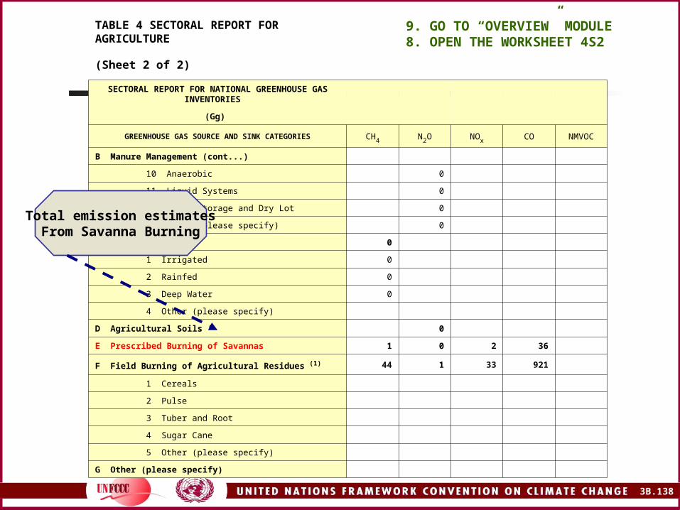
3B.138
9. GO TO “OVERVIEW” MODULE8. OPEN THE WORKSHEET 4S2
TABLE 4 SECTORAL REPORT FOR AGRICULTURE
(Sheet 2 of 2)
SECTORAL REPORT FOR NATIONAL GREENHOUSE GAS INVENTORIES
(Gg)
GREENHOUSE GAS SOURCE AND SINK CATEGORIES CH4 N2O NOx CO NMVOC
B Manure Management (cont...)
10 Anaerobic 0
11 Liquid Systems 0
12 Solid Storage and Dry Lot 0
13 Other (please specify) 0
C Rice Cultivation 0
1 Irrigated 0
2 Rainfed 0
3 Deep Water 0
4 Other (please specify)
D Agricultural Soils 0
E Prescribed Burning of Savannas 1 0 2 36
F Field Burning of Agricultural Residues (1) 44 1 33 921
1 Cereals
2 Pulse
3 Tuber and Root
4 Sugar Cane
5 Other (please specify)
G Other (please specify)
Total emission estimatesFrom Savanna Burning

3B.139
PRESCRIBED BURNING OF SAVANNAS
LTotal C released
(Gg C)from previous slide
NTotal N released
(Gg N)from previous slide
ON2O & NOx
emission rates
OCH4 & CO
emission rates
PN2O-N released
(Gg N)
PCH4-C released
(Gg C)
PNOx-N released
(Gg N)
PCO-C released
(Gg C)
QN2O & NOx
conversion rates
QCH4 & CO
conversion rates
R N2O emitted
(Gg N2O)
RNOx emitted
(Gg NOX)
RCH4 emitted
(Gg CH4)
RCO emitted
(Gg CO)
If no CS EFs,defaults in EFDB
Applicable to aggregated figures

3B.140
PRESCRIBED BURNING OF SAVANNASExamples of default emission factors

3B.141
PRESCRIBED BURNING OF SAVANNAS
Example based in a ficticious country having
three ecological regions: north, centre, south Northern zone: shortest drought period Southern zone: longest drought period Central zone: intermediate situation Two scenarios:
use of country-specific values for the majority of the ADs and EFs
use of default values for all the ADs and EFs

3B.142
PRESCRIBED BURNING OF SAVANNASEmission estimates using CS values
STEP 1 STEP 2
A B C D E F G H
Savanna category
Area Burned by Category (specify)
Biomass Density of Savanna
Total Biomass Exposed to Burning
Fraction Actually Burned
Quantity Actually Burned
Fraction of Living Biomass Burned
Quantity of Living Biomass Burned
Quantity of Dead Biomass Burned
(k ha) (t dm/ha) (Gg dm) (Gg dm) (Gg dm) (Gg dm)
C = (A x B) E = (C x D) G = (E x F) H = (E - G)
North15,5 7,00 108,50 0,85 92,23 0,55 50,72
41,50
Centre145,8 5,00 729,00 0,95 692,55 0,50 346,28
346,28
South22,0 4,00 88,00 1,00 88,00 0,45 39,60
48,40
Totals 436,60
436,18
AD from national statistics(census, surveys, mapping)
CS values(field measurements, expert’s
judgement)

3B.143
PRESCRIBED BURNING OF SAVANNASEmission estimates using CS values
STEP 3
I J K L
Savanna category
Biomass type
Fraction Oxidised of living and dead
biomass
Total Biomass
Oxidised
Carbon Fraction of Living & Dead
Biomass
Total Carbon
Released
(Gg dm) (Gg C)
Living: J = (G x I)
Dead: J = (H x I)
L = (J x K)
NorthLiving 0,9 37,35 0,4 14,94
Dead 0,95 48,19 0,45 21,68
CentreLiving 0,9 324,77 0,4 129,91
Dead 0,95 280,48 0,45 126,22
SouthLiving 0,9 41,38 0,4 16,55
Dead 0,95 35,74 0,45 16,08
TotalsLiving 403,50 325,39
Dead 364,41
CS values(field measurements, lab
analysis, expert’s judgement)

3B.144
PRESCRIBED BURNING OF SAVANNASEmission estimates using CS values
SUBMODULE PRESCRIBED BURNING OF SAVANNAS
WORKSHEET 4-3
SHEET 3 OF 3
COUNTRY CHILE
YEAR 2002
STEP 4 STEP 5
M N O P Q R
Nitrogen-
Carbon Ratio
Total Nitrogen Content
Emissions
Ratio
Emissions Conversion Ratio
Emissions from Savanna
Burning
(Gg N) (Gg C or
Gg N) (Gg)
N = (L x M) P = (L x O) R = (P x Q)
0,006 2,06 16/12 CH4 2,75
0,06 20,62 28/12 CO 48,11
0,0142 4,88 P = (N x O) R = (P x
Q)
0,006 0,03 44/28 N2O 0,05
0,121 0,59 46/14 NOx 1,94
CS values for CH4 & N2OD values for CO & NOx

3B.145
PRESCRIBED BURNING OF SAVANNASEmission estimates using default values
STEP 1 STEP 2
A B C D E F G H
Area Burned by Category
(specify)
Biomass
Density of
Savanna
Total Biomass Exposed to
Burning
Fraction
Actually
Burned
Quantity
Actually
Burned
Fraction of
Living
Biomass
Burned
Quantity of Living
Biomass
Burned
Quantity of
Dead Biomass
Burned
(k ha) (t dm/ha) (Gg dm) (Gg dm) (Gg dm) (Gg dm)
C = (A x B) E = (C x D) G = (E x F) H = (E - G)
15,50 7,00 108,50 0,95 103,08 0,55 56,69
EF ID= 43475 EF ID= 43485 EF ID= 43518 46,38
145,80 6,00 874,80 0,95 831,06 0,55 457,08
EF ID= 43445 EF ID= 43485 EF ID= 43518 373,98
22,00 4,00 88,00 0,95 83,60 0,45 37,62
EF ID= 43480 EF ID= 43485 EF ID= 43515 45,98
551,39
466,34
Default valuestaken from EFDB
AD fromnational statisitcs

3B.146
PRESCRIBED BURNING OF SAVANNASEmission estimates using default values
STEP 3
I J K L
Savanna category
Fraction Oxidised of living
and dead biomass
Total Biomass Oxidised
Carbon Fraction of Living & Dead
Biomass
Total Carbon
Released
(Gg dm) (Gg C)
Living: J = (G x I) Dead: J =
(H x I) L = (J x K)
NorthLiving 0,94 53,29 0,4 21,32
Dead 0,94 43,60 0,45 19,62
CentreLiving 0,94 429,66 0,4 171,86
Dead 0,94 351,54 0,45 158,19
SouthLiving 0,94 35,36 0,4 14,15
Dead 0,94 43,22 0,45 19,45
TotalsLiving 518,31 404,59
Dead 438,36
EF ID= 45949 Experts
Default valuestaken from EFDB
CS valuestaken from expert’s
judgement

3B.147
PRESCRIBED BURNING OF SAVANNASEmission estimates using default values
SUBMODULE PRESCRIBED BURNING OF SAVANNAS
WORKSHEET 4-3
SHEET 3 OF 3
COUNTRY CHILE
YEAR 2002
STEP 4 STEP 5
M N O P Q R
Nitrogen- Carbon Ratio
Total Nitrogen
Content
Emissions
Ratio
Emissions Conversion
Ratio
Emissions from
Savanna Burning
(Gg N)(Gg C or Gg
N)(Gg)
N = (L x M) P = (L x O) R = (P x Q)
0,005 2,02 16/12 CH4 2,70
0,06 24,29 28/12 CO 56,64
0,0095 3,84 P = (N x O) R = (P x Q)
EF ID= 45998 0,007 0,03 44/28 N2O 0,04
0,121 0,47 46/14 NOx 1,53
defaultsDefault values
taken from EFDB

3B.148
PRESCRIBED BURNING OF SAVANNASDifference of estimates
PRESCRIBED BURNING OF SAVANNAS
Emissions Emissions Per cent
Gas emitted Gg gas Gg gas of
using using difference
CS values Defaults
CH4 2,75 2,70 2%
CO 48,11 56,64 -15%
N2O 0,05 0,04 9%
NOx 1,94 1,53 27%

3B.149
RICE CULTIVATION

3B.150
RICE CULTIVATION Anaerobic decomposition of organic material in
flooded rice fields produces CH4
The gas escapes to the atmosphere primarily by transport through the rice plants
Amount emitted: function of rice species, harvests nº/duration, soil type, tº, irrigation practices, and fertilizer use
Three processes of CH4 release into the atmosphere: Diffusion loss across the water surface (least important
process) CH4 loss as bubbles (ebullition) (common and significant
mechanism, especially if soil texture is not clayey) CH4 transport through rice plants (most important
phenomenon)

3B.151
RICE CULTIVATIONMethodological issues
1996 IPCC Guidelines outline one method, that uses annual harvested areas and area-based seasonally integrated emission factors (Fc = EF x A x 10-12)
In its most simple form, the method can be implemented using national total area harvested and a single EF
High variability in growing conditions (water management practices, organic fertilizer use, soil type) will significantly affect seasonal CH4 emissions
Method can be modified by disaggregating national total harvested area into sub-units (e.g. areas under different water management regimes or soil types), and multiplying the harvested area for each sub-unit by an specific EF
With this disaggregated approach, total annual emissions are equal to the sum of emissions from each sub-unit of harvested area

3B.152
RICE CULTIVATIONActivity data
total harvested area excluding upland rice (national statistics or international databases FAO (www.fao.org/ag/agp/agpc/doc) or IRRI (www.irri.org/science/ricestat/pdfs)
harvested area differs from cultivated area according the number of cropping within the year (multiple cropping)
regional units, recognising similarities in climatic conditions, water management regimes, organic amendments, soil types, and others (national statistics or mapping agencies or expert judgement)
harvested area per regional unit (national statistics or mapping agencies)
cropping practices per regional unit (research agencies or expert judgement)
amount/type of organic amendments applied per regional unit, to allow the use of scaling factors (national statistics or international databases or expert judgement)

3B.153
RICE CULTIVATIONMain features from decision-tree (1)
If no rice is produced, then reported as “NO” If not key source:
and cropped area is homogeneous, then emissions can be estimated using total harvested area (Box 1)
but cropped area in heterogeneous, then total harvested area muts be disaggregated into homogeneous regional units applying default EF and scaling factors, if available
If keysource: and the cropped area is homogeneous, then emissions must be estimated using total
harvested area and CS EFs (Box 2) but cropped area variable, then the total harvested area must be divided into
homogeneous regional units and emissions estimated using CS EFs and scaling factors for organic ammendements (if available) (Box 3)
The country is encouraged to produce seasonally-integrated EFs for each regional unit (excluding organic ammendements) through a good practice measurement programme
The EFs must include the multiple cropping effect

3B.154
RICE CULTIVATIONNumerical example
Assumptions:
Hypothetical country located in Asia Key source condition Total harvested area: 38,5 kha, disaggregated
into: 28,5 kha as irrigated and continously flooded 10,0 kha as irrigated, intermitently flooded and
single aereated

3B.155
RICE CULTIVATION
MODULE AGRICULTURE
SUBMODULE METHANE EMISSIONS FROM FLOODED RICE FIELDS
WORKSHEET 4-2
SHEET 1 OF 1
COUNTRY FICTICIOUS LAND
YEAR 2002
A B C D E
Water Management Regime Harvested Area Scaling Factor for
Methane
Emissions
Correction Factor for
Organic Amendment
Seasonally Integrated
Emission Factor for
Continuously Flooded Rice without
Organic Amendment
CH4 Emissions
(m2 /1 000 000 000) (g/m2) (Gg)
E = (A x B x C x D)
Irrigated Continuously Flooded 0,285 1 2 20 11,40
Intermittently Flooded
Single Aeration 0,1 0,5 2 20 2,00
Multiple Aeration 0,00
Rainfed Flood Prone 0,00
Drought Prone 0,00
Deep Water
Water Depth 50-100 cm
0,00
Water Depth > 100 cm 0,00
Totals 0,385 13,40
AD from national statisticsor international databases
(FAO, IRRI)
Scaling factor for watermanagement: local research or
other country’s use or EFDB(Agriculture, Rice Production,
Intermitently Flooded, Single aeration)
Enhancement factor for organicammendements: local research or
taken from the EFDB(Agriculture, Rice Production)
EF: local researchor other country’s use
or from EFDBRegional units, fromnational estatistics ormapping agencies or
expert judgement