3.2 - 1 division algorithm let (x) and g (x) be polynomials with g (x) of lower degree than (x)...
TRANSCRIPT

3.2 - 13.2 - 1
Division Algorithm
Let (x) and g(x) be polynomials with g(x) of lower degree than (x) and g(x) of degree one or more. There exists unique polynomials q(x) and r(x) such that
where either r(x) = 0 or the degree of r(x) is less than the degree of g(x).
,x x x x f g q r

3.2 - 23.2 - 2
Synthetic Division
Synthetic division is a shortcut method of performing long division with polynomials.
It is used only when a polynomial is divided by a first-degree binomial of the form x – k, where the coefficient of x is 1.

3.2 - 33.2 - 3
Synthetic Division
3 24 3 2 0 150x x x x 3 23 12x x
23x
210 0x x
10x
210 40x x40 150x
40
40 160x 10
3.2 - 43.2 - 4
Synthetic Division
4 3 2 0 150 3 12
3
10 0
10
10 4040 150
40
40 16010
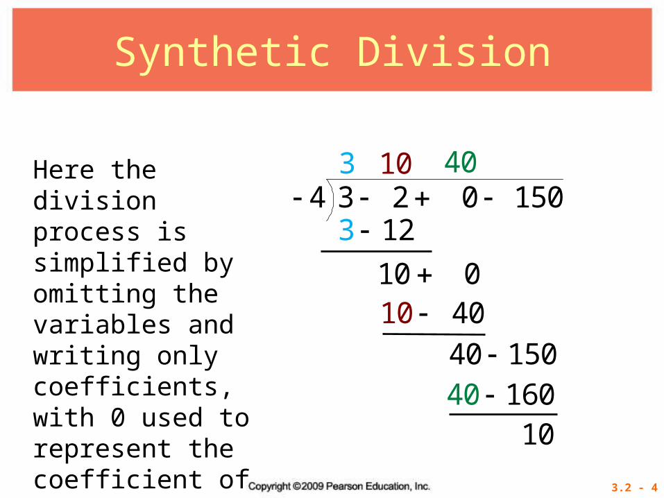
Here the division process is simplified by omitting the variables and writing only coefficients, with 0 used to represent the coefficient of any missing terms.

3.2 - 53.2 - 5
Synthetic Division
4 3 2 0 150 12
The numbers in color that are repetitions of the numbers directly above them can be omitted as shown here.
10 04040 150
16010
3 10 40

3.2 - 63.2 - 6
Synthetic Division
4 3 2 0 150 12
The entire problem can now be condensed vertically, and the top row is obtained by subtracting – 12, – 40, and – 160 from the corresponding terms above them.
40 160103 10 40

3.2 - 73.2 - 7
Synthetic Division
4 3 2 0 150 12
With synthetic division it is helpful to change the sign of the divisor, so the – 4 at the left is changed to 4, which also changes the sign of the numbers in the second row. To compensate for this change, subtraction is changed to addition.
40 160103 10 40
Additive inverse
Signs changed
23 10 4010
4x x
x
Quotient
Remainder

3.2 - 83.2 - 8
Caution To avoid errors, use 0 as the coefficient for any missing terms, including a missing constant, when setting up the division.

3.2 - 93.2 - 9
Example 1 USING SYNTHETIC DIVISION
Solution Express x + 2 in the form x – k by writing it as x – (– 2). Use this and the coefficients of the polynomial to obtain
Use synthetic division to divide 3 25 6 28 2
.2
x x xx
2 5 6 28 2. x + 2 leads to – 2
Coefficients

3.2 - 103.2 - 10
Example 1 USING SYNTHETIC DIVISION
Solution Add – 2 and – 8 to obtain – 10.
Use synthetic division to divide 3 25 6 28 2
.2
x x xx
2 5 6 28 2
51016
324
810 Remainder
Quotient

3.2 - 113.2 - 11
Example 1 USING SYNTHETIC DIVISION
Since the divisor x – k has degree 1, the degree of the quotient will always be written one less than the degree of the polynomial to be divided. Thus,
Use synthetic division to divide 3 25 6 28 2
.2
x x xx
22
3
51
16 45 6 28 2 0
2.
2x
xx
xx
xx
Remember to add remainder
.divisor
3.2 - 123.2 - 12
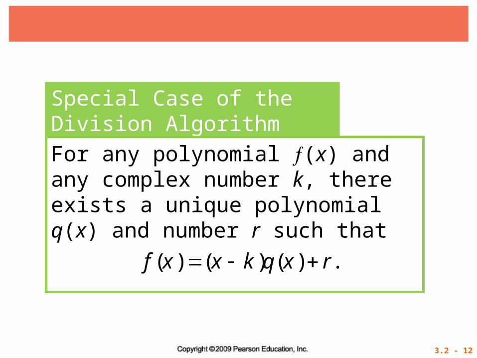
Special Case of the Division Algorithm
For any polynomial (x) and any complex number k, there exists a unique polynomial q(x) and number r such that
( ) ( ) ( ) .x x k q x r f

3.2 - 133.2 - 13
For Example
In the synthetic division in Example 1,
3 2 25 6 28 2 ( 2)(5 16 4) ( 10).x x x x x x
( )xf ( )x k ( )xq r
Here g(x) is the first-degree polynomial x – k.

3.2 - 143.2 - 14
Remainder Theorem
If the polynomial (x) is divided by x – k, the remainder is equal to (k).

3.2 - 153.2 - 15
Remainder Theorem
In Example 1, when (x) = 5x3 – 6x2 – 28x – 2 was divided by x + 2 or x –(– 2), the remainder was – 10. Substituting – 2 for x in (x) gives
3 2( ) 5( ) 6( ) 28(2 2)2 22 f
40 24 56 2 10 Use parentheses
around substituted values to avoid errors.

3.2 - 163.2 - 16
Remainder Theorem
A simpler way to find the value of a polynomial is often by using synthetic division. By the remainder theorem, instead of replacing x by – 2 to find (– 2), divide (x) by x + 2 using synthetic division as in Example 1. Then (– 2) is the remainder, – 10.
2 5 6 28 2
51016
324
810 (– 2)

3.2 - 173.2 - 17
Example 2 APPLYING THE REMAINDER THEOREM
Solution Use synthetic division with k = – 3.
Let (x) = – x4 + 3x2 – 4x – 5. Use the remainder theorem to find (– 3).
3 1 0 3 4 5 3 9 18 42
1 3 6 1 474 Remainder
By this result, (– 3) = – 47.

3.2 - 183.2 - 18
Testing Potential Zeros
A zero of a polynomial function is a number k such that (k) = 0. The real number zeros are the x-intercepts of the graph of the function.
The remainder theorem gives a quick way to decide if a number k is a zero of the polynomial function defined by (x). Use synthetic division to find (k); if the remainder is 0, then (k) = 0 and k is a zero of (x). A zero of (x) is called a root or solution of the equation (x) = 0.

3.2 - 193.2 - 19
Proposed zero
Example 3 DECIDING WHETHER A NUMBER IS A ZERO
Solution
a.
Decide whether the given number k is a zero of (x).
3 2( ) 4 9 6; 1x x x x k f
1 1 4 9 6 1 3 6
1 3 6 0
3 2( ) 4 9 6x x x x f
Remainder
Since the remainder is 0, (1) = 0, and 1 is a zero of the polynomial function defined by (x) = x3 – 4x2 + 9x – 6. An x-intercept of the graph (x) is 1, so the graph includes the point (1, 0).

3.2 - 203.2 - 20
Proposed zero
Example 3 DECIDING WHETHER A NUMBER IS A ZERO
Solution Remember to use 0 as coefficient for the missing x3-term in the synthetic division.
b.
Decide whether the given number k is a zero of (x).
4 2( ) 3 1; 4x x x x k f
4 1 30 1 1 4 16 68 284
Remainder1 2854 17 71 The remainder is not 0, so – 4 is not a zero of (x) = x4 +x2 – 3x + 1. In fact, (– 4) = 285, indicating that (– 4, 285) is on the graph of (x).