3.13 solutions of exercises - cvut.czfsinet.fsid.cvut.cz/en/u2052/statics_part_two.pdf · 3.13...
TRANSCRIPT

CHAPTER 3. STATICS 132
3.13 Solutions of exercises
Solution of Exercise 3.3.2
N
G
P
S2
S1
â
á
Figure 3.86: Exercise 3.3.2. Free-body diagram
Forces in springs:
S1 = k1(ql201 + x2 � l01)
S2 = k2(ql202 + x2 � l02)
Geometry:
sin� =l01pl201 + x2
; cos� =xp
l201 + x2
sin � =l02pl202 + x2
; cos � =xp
l202 + x2
Equations of equilibrium:
P � S1 cos�� S2 cos � = 0
N + S1 sin��G� S2 sin� = 0
Solution:P = S1 cos� + S2 cos �
Result:P = 77:6 N
Notice: The second equation of equlibrium is not necessary for finding the forceP . It can be used for determination of the reaction forceN .

CHAPTER 3. STATICS 133
Solution of Exercise 3.3.3
N
W
W2W1
á â
Figure 3.87: Exercise 3.3.3. Free-body diagram
Geometry:
sin� =hp
h2 + x2; cos� =
xph2 + x2
sin� =hp
(l � x)2 + h2; cos � =
l � xp(l � x)2 + h2
Equations of equilibrium:
W2 cos � �W1 cos� = 0
N +W1 sin� +W2 sin� �W = 0
Solution:
W2l � xp
(l � x)2 + h2�W1
xph2 + x2
= 0 => xeq
Notice: See Matlab fileS213.m for numerical solution.

CHAPTER 3. STATICS 134
Solution of Exercise 3.3.4
G
P
Nn
t
á
á
Figure 3.88: Exercise 3.3.4. Free-body diagram
Geometry:
y =b
a2x2
y0 = tan� =2b
a2x
Equations of equilibrium:
P cos��G sin� = 0
N �G cos�� P sin� = 0
From equation of equilibrium we have:
tan� =P
G
Solution:
xeq =a2
2b
P
G
Result:xeq = 0:036 m

CHAPTER 3. STATICS 135
Solution of Exercise 3.3.5
G
F
Sn
t
á
áá
Figure 3.89: Exercise 3.3.5. Free-body diagram
Geometry:
tan� =xeqpl2 � x2eq
Equations of equilibrium:
F cos��G sin� = 0
S �G cos�� F sin� = 0
Solution:
tan� =xeqpl2 � x2eq
=F
G! xeq
Notice:See Matlab fileS216.m for numerical solution.

CHAPTER 3. STATICS 136
Solution of Exercise 3.4.2
a a
M
A
RAx
RAy
SG
W = ½ a wo
2/3 a
Figure 3.90: Exercise 3.4.2. Free-body diagram
Equations of equilibrium:PFix : RAx = 0PFiy : RAy + S �W �G = 0PMiA : �Ga�W 5
3a+ S 2 a+M = 0
Solution:
S =1
2G+
5
6W � M
2 a
l0 = 0:5 a+ � = 0:5 a+S
k
RA = RAy = G+W � S
Result:S = 603:4 N
l0 = 0:112 m
RA = 396:6 N

CHAPTER 3. STATICS 137
Solution of Exercise 3.4.3
Rx
Ry
G
S
á
Figure 3.91: Exercise 3.4.3. Free-body diagram
Geometry:
sin� =ap
4 a2 + a2=
1p5
Equations of equilibrium:PFix : Rx � S cos� = 0PFiy : Ry + S sin� � G = 0PMiA : S sin� 2 a�Ga = 0
Solution:
S =G
2 1p5
=
p5
2G
k =S
�=
S
ap5� 2 a
=167:7
0:15p5� 0:3
Result:S = 167:7 N
k = 4737 Nm�1

CHAPTER 3. STATICS 138
Solution of Exercise 3.4.4
G1
a d1,5 a
G2
NfNr
A B
Figure 3.92: Exercise 3.4.4. Free-body diagram
Equations of equilibrium:PMiA : Nf 2:5 a�G1 1:5 a�G2 (2:5 a+ d) = 0PMiB : G1 a�Nr 2:5 a�G2 d = 0
Solution:
Nf =1:5G1 a+ (2:5 a+ d)G2
2:5 a
Nr =G1 a+G2 d
2:5 a
Result:Nf = 6700 N
Nr = 300 N

CHAPTER 3. STATICS 139
Solution of Exercise 3.4.5
G2
a N2
G1 G
d c
b
N1
A B
Figure 3.93: Exercise 3.4.5. Free-body diagram
a) Minimum counterweightG1min for the crane not to lose its stability withG2 = 0 . We supposeN1 = 0 :
Equations of equilibrium:PMiB : G1min (d+
a2)�G (b� a
2) = 0
Solution:
G1min =b� a
2
d+a2
G = 1538 N
b) Maximum weightG2max = 0 for the crane not to loose its stability withG1max.
First we determineG1max from the conditionN2 = 0, G2 = 0. Equations ofequilibrium: P
MiA : G1max (d� a2)�G(b + a
2) = 0
G1max =b+ a
2
d� a2
G = 11428 N
Now we findG2max supposingN1 = 0.Equations of equilibrium:P
MiB : G1max (d+a2)�G (b� a
2)�G2max (c� a
2) = 0

CHAPTER 3. STATICS 140
Solution:
G2max =G1max (d+
a2)�G (b� a
2)
c� a2
= 3475 N

CHAPTER 3. STATICS 141
Solution of Exercise 3.5.2
Β″
b
T2
″
T1
″
a
F″
A″
Q″
G″
a1/5
T1
″′
T2
″′
G″′
F″′Q″′
30º
20º
z
y′
z′
x
Q
RAy
F
RAx
RAz
y
RBy
RBz
G T1
T2
aa
Figure 3.94: Exercise 3.5.2. Free-body diagram
Equations of equilibrium in a scalar form:PFix : RAx = 0PMix : (T2 � T1) a+ F 0:2 a = 0PMiy : T2 b +RAz (a+ b) + T1 cos 30
Æ b�Qa cos 20Æ = 0PMiz : �F a+Qa sin 20Æ � RAy (a+ b)� T1 b sin 30
Æ +G1 b = 0PMiy0 : �T2 a� T1 a cos 30Æ � RBz (a + b)�Q (a+ b + a) cos 20Æ = 0PMiz0 : �G1 a+ T1 a sin 30Æ +RBy (a+ b)� F (a+ b+ a) +Q (a+ b + a) sin 20Æ = 0
Equation of equilibrium in matrix form:26666664
1 �5 0 0 0 0�a a 0 0 0 0
b cos 30Æ b 0 a+ b 0 0�b sin 30Æ 0 �a� b 0 0 0�a cos 30Æ �a 0 0 0 �a� ba sin 30Æ 0 0 0 a+ b 0
37777775
26666664
T1T2RAy
RAz
RBy
RBz
37777775=

CHAPTER 3. STATICS 142
26666664
0�F 0:2 aQa cos 20Æ
F a�Qa sin 20Æ �G1 bQ (a+ b + a) cos 20Æ
G1 a+ F (a+ b+ a)�Q (a + b+ a) sin 20Æ
37777775
Result:RAx = 0 N, RAy = �946:2 N, RAz = �860 N, RA = 12786 N, RBy = 4349:4 N,RBz = �581:9 N, RB = 43881 N, T1 = 10000 N, T2 = 2000 N
Notice: See Matlab fileS3415.m for numerical solution.

CHAPTER 3. STATICS 143
Solution of Exercise 3.5.3
A″
a
r
4r
2a5a
z
y
T2
″
T1
″
N″
T2
″′
T1
″′N″′
≡Β″′A″′
S″′
x
y’ y
RByRAy
RAx
RAy,
RAz,
RBy,
RBzΒ″
S″
á
Figure 3.95: Exercise 3.5.3. Free-body diagram
Equations of equilibrium in scalar form:PFix : RAx + T2 = 0PMix : S cos� r � T1 4r = 0PMiy : RBz 5a � T1 2a + S cos� 6a = 0PMiz : �RBy 5a + S sin� 6a + N 2a + T2 4r = 0PMiy0 : �RAz 5a + S cos� a � T1 7a = 0PMiz0 : RAy 5a + S sin� + N 7a + T2 4r = 0
Equation of equilibrium in matrix form:26666664
1 0 0 0 0 00 0 0 0 0 cos�0 0 0 0 5 6 cos�0 0 0 �5 0 6 sin�0 0 �5 0 0 cos�0 5 0 0 0 sin�
37777775
26666664
RAx
RAy
RAz
RBy
RBz
S
37777775=
26666664
�T24T12T1
�2N � 4:08T27T1
�7N � 4:08T2
37777775
Notice: See Matlab fileS3421.m for numerical solution.

CHAPTER 3. STATICS 144
Solution of Exercise 3.5.4
r
ϕ
Q
G
RC
RA
RB
ϕ
x
R
30
30ο
ο
y
z
Figure 3.96: Exercise 3.5.4. Free-body diagram
Equations of equilibrium:PFiz : �Q�G+RA +RB +RC = 0PMix : �Qr sin'+RBR cos 30Æ � RCR cos 30Æ = 0PMiy : Qr cos'�RAR +RBR sin 30Æ + RCR sin 30Æ = 0
Solution:RA = Q +G� (RB +RC)
RB � RC =Qr sin'
R cos 30Æ= f1(')
RB +RC =(Q +G)R�Qr cos'
R (1 + sin 30Æ)= f2(')
RB =f1(') + f2(')
2
RC =f2(')� f1(')
2
Notice: See Matlab fileS3423.m for numerical solution.
CHAPTER 3. STATICS 145
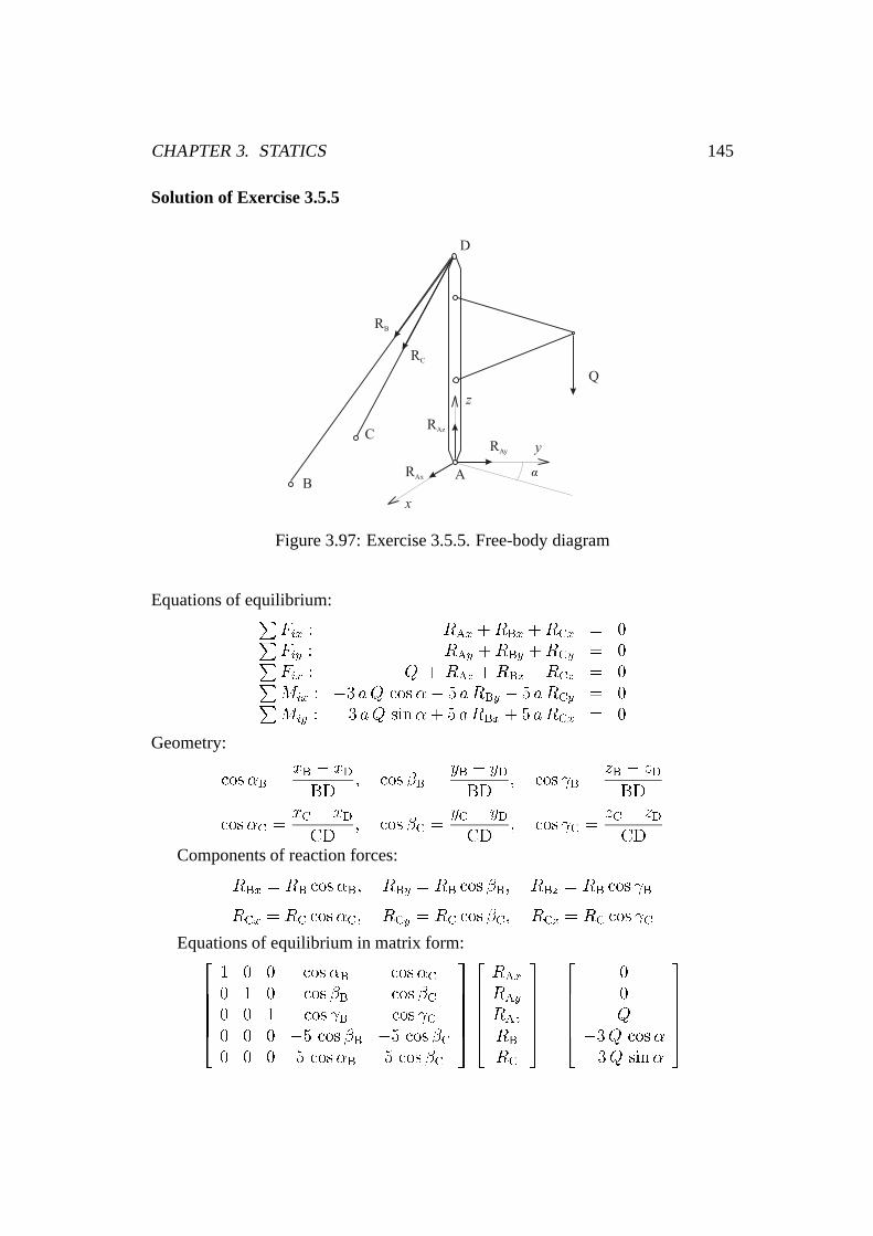
Solution of Exercise 3.5.5
x
BA
y
z
Q
RAx
RAy
RAz
RB
RC
C
D
á
Figure 3.97: Exercise 3.5.5. Free-body diagram
Equations of equilibrium:PFix : RAx +RBx +RCx = 0PFiy : RAy +RBy +RCy = 0PFix : �Q + RAz +RBz +RCz = 0PMix : �3 aQ cos�� 5 aRBy � 5 aRCy = 0PMiy : 3 aQ sin�+ 5 aRBx + 5 aRCx = 0
Geometry:
cos�B =xB � xDBD
; cos �B =yB � yDBD
; cos B =zB � zDBD
cos�C =xC � xDCD
; cos �C =yC � yDCD
; cos C =zC � zDCD
Components of reaction forces:
RBx = RB cos�B; RBy = RB cos �B; RBz = RB cos B
RCx = RC cos�C; RCy = RC cos �C; RCz = RC cos C
Equations of equilibrium in matrix form:2666641 0 0 cos�B cos�C0 1 0 cos �B cos �C0 0 1 cos B cos C0 0 0 �5 cos �B �5 cos �C0 0 0 5 cos�B 5 cos �C
377775
266664RAx
RAy
RAz
RB
RC
377775 =
266664
00Q
�3Q cos��3Q sin�
377775
CHAPTER 3. STATICS 146
Notice: See Matlab fileS3410.m for numerical solution.

CHAPTER 3. STATICS 147
Solution of Exercise 3.5.6
y
z
Q”
Β”
Q’ ≡ Β’
y
x
B”
A″
S”1S”2
G”
D” E”RAy
RAy
RAz
RAx
S’1
S’2
C’
G’ E’
B’
A’ D’
C”
Figure 3.98: Exercise 3.5.6. Free-body diagram
Equations of equilibrium:PFix : RAx + S1x + S2x = 0PFiz : RAy + S1y + S2y = 0PFiy : RAz + S1z + S2z �Q�G = 0PMix : �4 aQ+ a S1z + 3 a S2z � 2 aG = 0PMiz : �a S1x � 3 a S2x = 0
Geometry:
cos�DB =xB � xDDB
; cos �DB =yB � yDDB
; cos DB =zB � zDDB
cos�EC =xC � xEEC
; cos �EC =yC � yEEC
; cos EC =zC � zEEC

CHAPTER 3. STATICS 148
Components of forces:
S1x = S1 cos�DB; S1y = S1 cos �DB; S1z = S1 cos DB
S2x = S2 cos�EC; S2y = S2 cos �EC; S2z = S2 cos EC
Equations of equilibrium in matrix form:266664
1 0 0 cos�DB cos�EC0 1 0 cos �DB cos �EC0 0 1 cos DB cos EC0 0 0 cos DB 3 cos EC0 0 0 cos�DB 3 cos�EC
377775
266664RAx
RAy
RAz
S1S2
377775 =
266664
00
G+Q2G+ 4Q
0
377775
Notice: See Matlab fileS3411.m for numerical solution.

CHAPTER 3. STATICS 149
Solution of Exercise 3.5.7
≡ Β”A”
N
S”
T”2
A’
S’
xT’1
T’2
z
T”1
, z’
, RBz
y
B’ y’
RAz
RBx
RBy
RAy
Figure 3.99: Exercise 3.5.7. Free-body diagram
Equations of equilibrium:PFix : RBx + T1 = 0PMix : �2 a S + 3 aN + r T2 = 0PMiy : aN � r T1 � 2 a S + 2 aRBz = 0PMiz : �3 a T1 � a T2 � 2 aRBy = 0PMiy0 : �aN � r T1 � 2 aRAz = 0PMiz0 : a T2 � 3 a T1 + 2 aRAy = 0
Equations of equilibrium in matrix form:26666664
0 0 1 0 0 00 0 0 0 0 20 0 0 0 2 �20 0 0 �2 0 00 �2 0 0 0 02 0 0 0 0 0
37777775
26666664
RAy
RAz
RBx
RBy
RBz
S
37777775=
26666664
�T13N + 3:5T23:5T1 �N3T1 + T2
�N � 3:5T13T1 � T2
37777775
Notice: See Matlab fileS3422.m for numerical solution.

CHAPTER 3. STATICS 150
Solution of Exercise 3.6.2
RAy
RAx
RE
B
M4
2
3
D
C
4
F4
A
¾ a
a
a
b
2
A
y
RB
B
3
D
x
RB
B
3
D
C
RDy
RDx
d
c
F4
M4
C
4
F4
C
RCx
RCx
RCy
RCy
M4
ME
á
á
â
Figure 3.100: Exercise 3.6.2. Equilibrium of a structure
The structure has zero degree of freedom and it consists of three members. Wesketch the free-body diagram for the structure as a whole, and for members 3, 4.Than, we write 3 equilibrium equations for each free structure or body. We have

CHAPTER 3. STATICS 151
Structure as a whole:PFix : RAx = 0PFiy : RAy +RB � F4 = 0PMiB : RAy � a� F4 � 3=4 a+M4 = 0
Member 3: PFix : RDx +RCx = 0PFiy : RDy +RCy +RB = 0PMiC : RB d�RDy (c� d)�RDx (a� b) = 0
Member 4: PFix : �RCx �RE sin� = 0PFiy : RE cos�� RCy � F4 = 0PMiC : ME + F4 (3=4 a� d)�M4 = 0
Geometry yields
c = a� a
tg�; d =
b
tg�; � = arctg
a
c
Equation of equlibrium in matrix form:266666666664
1 1 0 0 0 0 0 0a 0 0 0 0 0 0 00 0 1 0 1 0 0 00 1 0 1 0 1 0 00 d 0 0 b� a d� c 0 00 0 1 0 0 0 sin� 00 0 0 �1 0 0 cos� 00 0 0 0 0 0 0 1
377777777775
266666666664
RAy
RB
RCx
RCy
RDx
RDy
RE
ME
377777777775=
266666666664
F434aF4 �M4
0000F4
F4 (d� 34a) +M4
377777777775
Notice: See Matlab fileSSB612.m for numerical solution.

CHAPTER 3. STATICS 152
Solution of Exercise 3.6.3
RAy
RAx
2
1
F
F
c
2
F
x
y
B
3
4D
E
Ad
d
a b b
RC
C
Q
Q
RBx
RBy
3
4
RDx
RDx
RDy
RDy
RC
RE
Figure 3.101: Exercise 3.6.3. Equilibrium of the pliers
We free bodies 2, 3, 4 and write the particular equations of equilibrium.Member 2: P
Fix : RAx +RDx = 0PFiy : �RDy +RAy � RC � F = 0PMiA : RDx d+RDy b�RC b� F (b + c) = 0

CHAPTER 3. STATICS 153
Member 3: PFix : RBx = 0PFiy : Q +RBy + RC = 0PMiB : 2 bRC �Qa = 0
Member 4: PFix : RDx = 0PFiy : �Q +RDy �RE = 0PMiD : Qa� 2 bRE = 0
Remark:You can see that it is not necessary to free the member 4. It is clear thatRDx = RBx; RDy = RBy; RC = RE from symmetry.
Using symmetry and excluding trivial scalar equations we have a system of only6 equilibrium equation. These are in matrix form:2
6666664
1 0 1 0 0 00 1 0 �1 �1 �10 0 d b �b �(b + c)0 0 0 �1 1 00 0 0 0 2 b 00 0 0 1 �1 0
37777775
26666664
RAx
RAy
RDx
RDy
RC
F
37777775=
26666664
000�QaQQ
37777775
Notice: See Matlab fileSSB614.m for numerical solution.

CHAPTER 3. STATICS 154
Solution of Exercise 3.6.4
B
l1
h1
∅ d
p
h
RBy
2
2
3
Fp
Fp
RBxN
l
C
4
D3
4
RDx
RDy
RDy
RDx
RCy
5
RE
RE
G
A6
QN
E
F4
5
G
6
Q
RF
RF
RCx
RAy
RAx
n
z1
z2
z3
s
á
ä
ä
Figure 3.102: Exercise 3.6.4. Equilibrium of the landing gear
First of all we expres the geometrical dependancies.
z1 = ECcosÆ ; z2 = AF cos� z3 = AGcos�
Next we free bodies 2, 3, 4, 5, 6 and write the particular equations of equilib-rium.Member 2: P
Fix : �RBx � Fp = 0PFiy : RBy +N = 0PMiB : N n = 0
Member 3: PFix : Fp +RDx = 0PFiy : �N +RDy = 0PMiD : N n = 0

CHAPTER 3. STATICS 155
Member 4: PFix : �RDx +RCx = 0PFiy : �RE � RDy +RCy = 0PMiC : RDx h1 +RE z1 = 0
Member 5: PFiy : RE � RF = 0
Member 6: PFix : �RAx = 0PFiy : RAy +RF �Q = 0PMiA : RF � z2 �Qz3 = 0
Remark: You can see that it is not necessary to determinate angle� . The lastequations can be rewriten to
RF = QAF
BF
.
Excluding trivial scalar equations we have system of only 8 equilibrium equa-tion. These are in matrix form:2
66666666664
0 �1 0 0 0 0 0 �10 0 0 0 1 0 0 10 0 1 0 �1 0 0 00 0 0 1 0 �1 0 00 0 0 0 h1 z1 0 00 0 0 0 0 1 �1 01 0 0 0 0 1 1 00 0 0 0 0 0 1 0
377777777775
266666666664
RAz
RBx
RCx
RCy
RDx
RE
RF
RFp
377777777775=
266666666664
000000Q
Qz3=z2
377777777775
The preasure can be computed from equation:
p =Fp�d2
4.
Notice:See Matlab fileS615.m for numerical solution.

CHAPTER 3. STATICS 156
Solution of Exercise 3.6.5
s t
x n
v
2
REx
2REy
5
3
RH
RH
B DC
r
Z 35
6
Z
6
RC
RD
RD
RC
RB
G
E
4
4
RK
RK
RG
RG
Q
Q
Figure 3.103: Exercise 3.6.5. Equilibrium of the decimal scales
We free bodies 2, 3, 4, 5, 6 and write the particular equations of equilibrium.Member 2: P
Fix : REx = 0PFiy : RG +REy +RH = 0PMiH : RG (v � s� t� u) +REy (v � s� t) = 0
Member 3: PFiy : RD � RH = 0

CHAPTER 3. STATICS 157
Member 4:PFiy : �RG +RK �Q = 0PMiK : �RGy (v � s� u)�Q (v � s� u� x) = 0
Member 5: PFiy : RC � RK = 0
Member 6: PFiy : �Z +RB � RC � RD = 0PMiB : Z r �RC s� RD (s+ t) = 0
Excluding trivial scalar equations we have system of only 8 equilibrium equa-tion. These are in matrix form:
266666666664
0 0 0 1 1 1 0 00 0 0 v � s� t v � s� t� u 0 0 00 0 1 0 0 1 0 00 0 0 0 �1 0 1 00 0 0 0 v � s� u 0 0 00 1 0 0 0 0 1 01 �1 1 0 0 0 0 00 �s �(s + t) 0 0 0 0 0
377777777775
266666666664
RB
RC
RD
REy
RG
RH
RK
Z
377777777775=
266666666664
000Q
Q (v � s� u� x)0ZZ r
377777777775
Notice:See Matlab fileS6111.m for numerical solution..

CHAPTER 3. STATICS 158
Solution of Exercise 3.6.6
2
RAx
RAy
D
E
½ l
l
l2
Aϕ
3
RDx RDx
RDy
RDy
RE
ϕ
½ a
a
BC
3
4
4
RCx
RCy
RCy
RCx
G
FP
FP
RB
RB
ã
ã
Figure 3.104: Exercise 3.6.6. Equilibrium of the lifting platform
First we express the geometrical dependancies:
� =
r(l +
l
2)2 + a2 � 2a(l +
l
2)cos�
= acos((l + l
2) � cos�� a
�)
� = �

CHAPTER 3. STATICS 159
Next we free bodies 2, 3, 4, and write the particular equations of equilibrium.Member 2: P
Fix : RAx +RDx = 0PFiy : RAy +RDy � RB = 0PMiA : RB 2lcos�� RDy lcos�� RDx lsin� = 0
Member 3:PFix : RCx � RDx + Fp cos = 0PFiy : RCy �RDy +RE + Fp sin = 0PMiC : RDy lcos�� RDx lsin�� RE 2lcos�� Fp sin( � �) l
2= 0
Member 4: PFix : �RCx � Fp cos = 0PFiy : �RCy � RB � Fp sin = 0PMiC : �RB 2lcos�+ Fp sin a = 0
We have system of only 9 equilibrium equation.If we introduce auxiliary variables:
cp = cos�; sp = sin�; cg = cos ; sg = sin ; se = sin�
Can be equations of equlibrium writen in matrix form:
26666666666664
1 0 0 0 0 1 0 0 00 1 �1 0 0 0 1 0 00 0 2lcp 0 0 �lsp �lcp 0 00 0 0 1 0 �1 0 0 cg0 0 0 0 1 0 �1 1 sg0 0 0 0 0 �lsp lcp �2lcp �se (l + l
2)
0 0 0 �1 0 0 0 0 �cg0 0 1 0 �1 0 0 0 �sg0 0 �2lcp 0 0 0 0 0 sg a
37777777777775
26666666666664
RAx
RAy
RB
RCx
RCy
RDx
RDy
RE
Fp
37777777777775=
26666666666664
0000000G
�Qa2
37777777777775
Notice:See Matlab fileS6120.m for numerical solution.

CHAPTER 3. STATICS 160
Solution of Exercise 3.6.7
D
C
E2
34
K
O AG2
B
F
RE4
K
2
G2
B
FRD
3
RD
RCy
RCx
RCx
RCy
RAy
RAx
á
å
Figure 3.105: Exercise 3.6.7. Equilibrium of a hub lifting mechanism
First we express the geometrical dependancies:
� = acos((OB2 +OA2 � AB2)
2 OB OA)
Æ = acos((AC2 +AB2 � BC2)
2 AC AB)
� = asin(OB
AB sin�)
� = � � Æ
Next we free bodies 2, 4, and write the particular equations of equilibrium.Member 2:P
Fix : RAx � RCx + F cos� = 0PFiy : RAy +RCy + F cos� �G2 = 0PMiA : RCxACcos�� RCy AC sin�� F cos�AB sin� � F sin�ABcos� = 0

CHAPTER 3. STATICS 161
Member 4: PFix : RCx +RD cos� = 0PFiy : �RCy � RD sin�� Z4 = 0PMiC : Z4CK� RD cos�CD = 0
We have system of only 6 equilibrium equation.If we introduce auxiliary variables:
mf = �cos�AB sin� � sin�ABcos�
Can be equations of equlibrium writen in matrix form:
26666664
1 0 �1 0 0 cos�0 1 0 1 0 sin�0 0 AC sin� �AC cos� 0 mf0 0 1 0 cos� 00 0 0 �1 �sin� 00 0 0 0 �cos� CD 0
37777775
26666664
RAx
RAy
RCx
RCy
RD
F
37777775=
26666664
0G2
�G2 ABcos�0Z4
�Z4CK
37777775
Notice:See Matlab fileS6122.m for numerical solution.
CHAPTER 3. STATICS 162
Solution of Exercise 3.8.2
v
G2
y
,e
r
l1
2
3
l
h
G3
F
G3
F
A
A
G2
Mt
RAx
RAy
x
N
Fsf
RAx
RAy
,rj
Mkj
Mkj
kjìsì
ø
ø
â
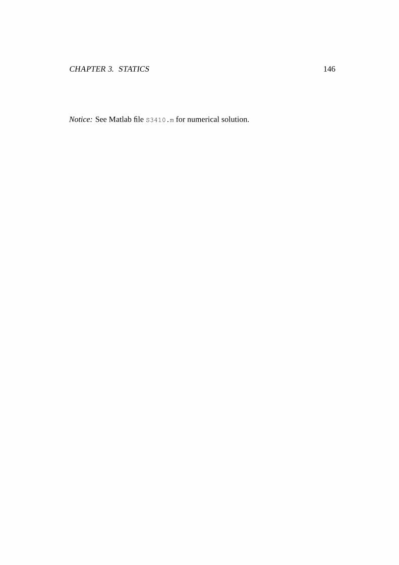
Figure 3.106: Exercise 3.8.2. Equilibrium of a hand-barrow
First we free particular bodies and write down the equations of equilibrium.Body 2: P
Fix : RAx � Fsf = 0PFiy : RAy �G2 +N = 0PMiA : Mkj +Mt � Fsf r = 0
Body 3:PFix : F cos � RAx = 0PFiy : �RAy �G3 + F sin = 0PMiA : F sin l cos � � F cos l sin � �G3 (l1 cos � � h sin�)�Mkj = 0
Then we express the friction forces using their definitions
Mkj = rj �kj
qR2Ax +R2
Ay ; Mt = jN j e

CHAPTER 3. STATICS 163
and we subsitute them into the equations of equilibrium. We get a system of 6nonlinear algebraic equation containing 6 unknownsRAx, RAy, Fsf , N , F , . Wesolve the system using Matlab. The result isF= 154.7 N, = 84:7Æ.
After the solution we check the condition of rolling using the formula
jFsf j � jN j�s :
The condition is valid in our case because14:34 < 144:36.In case we have no solver for system of nonlinear algebraic equations we can
use the linearized expression
Mkj = rj �kj (0:96 jRAyj+ 0:4 jRAxj)
for the moment of friction. Supposing
jRAyj > jRAxj
we get a system of 6 linear algebraic equations after linearizing. These can bewritten and solved using familiar approach.
Solution of linearizing equations:F = 149:53 N, = 88:88Æ
Solution of nonlinearizing equations:F = 158:18 N, = 82:33Æ
CHAPTER 3. STATICS 164
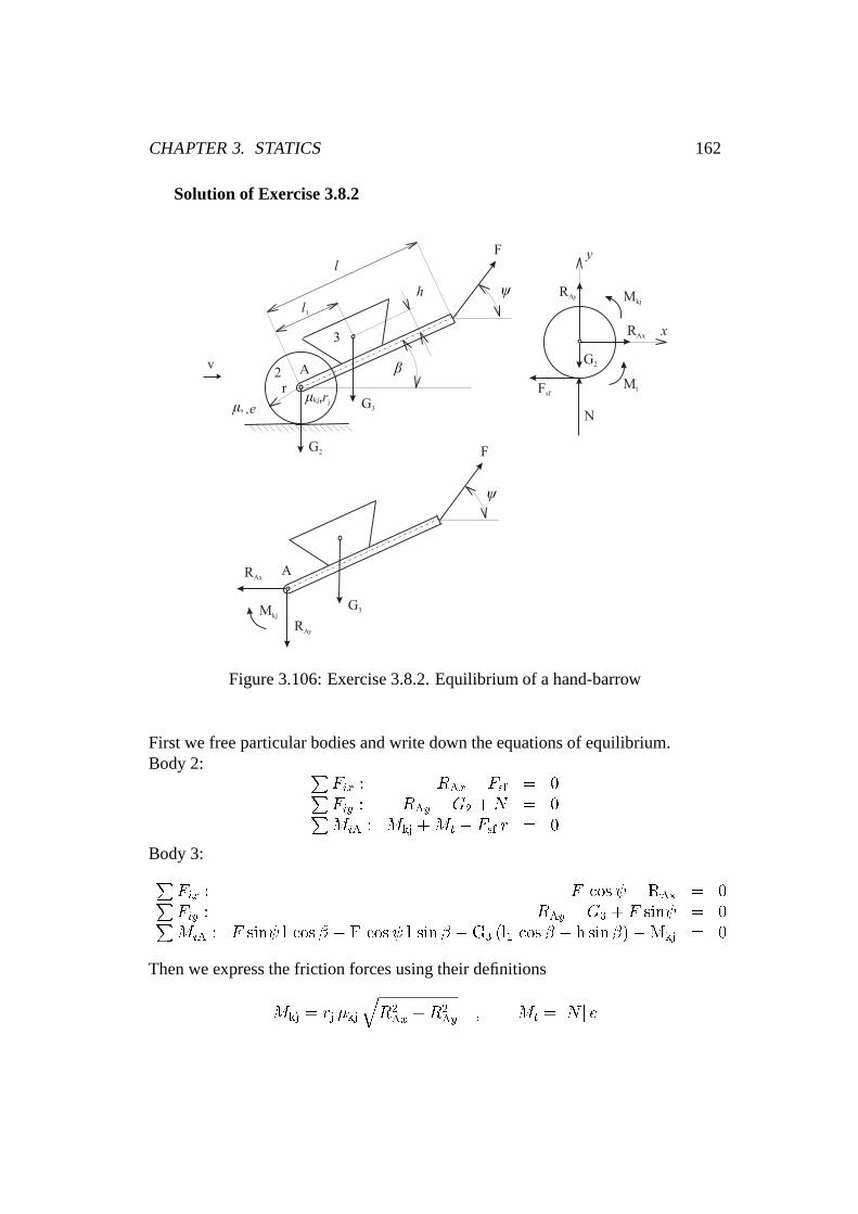
Solution of Exercise 3.8.3
M
Q
rQ
ϕ
R
2Q
QRx
Ry
áâ
ã
kì
Figure 3.107: Exercise 3.8.3. Free-body diagram
First we use the standard expression for belt friction:
2Q
Q= e� �k
This yieldsln2 = � �k
� =1
�kln2 = 2:310 rad = 132:353Æ
From geometry we have
cos� =R
r
� = arccosR
r= 60Æ
' = � + � = 192:353Æ
= '� 180Æ = 12:353Æ
Equilibrium equation is
M +QR�Qr cos = 0
This yieldsM = Q (r cos � R) = 9:54 Nm

CHAPTER 3. STATICS 165
Solution of Exercise 3.8.4
r
2
R
OOO
M
S1
S1
S2
S2
S
Mkj1
Mkj2
k =ì sì
k =ì sì
Figure 3.108: Exercise 3.8.4. Free-body diagram
Equations of equilibrium for the upper wheel:
S = S1 + S2rj �kj (S1 + S2) = (S1 � S2) r
Equations of equilibrium for the lower wheel:
R = S1 + S2 +OM = (S1 +O � S2) r + rj �kj (S1 + S2 +O)
Expression for the belt friction:
S1 +O
S2= e� �k ! min
Altogether we have 5 equations for 5 unknowns, namelyS; S1; S2; R;M . Aftersome manipulations we have
S2 =rj �kj�r
rc �kj (e� �k+1)�r (e� �k�1)] O = 123:1 N
S1 = S2 e� �k � O = 130:74N
S = S1 + S2 = 253:846 NM = 23:652 NmR = S1 + S2 +O = 353:84 N

CHAPTER 3. STATICS 166
Solution of Exercise 3.8.5
Q
l
l
G
N
N N N
N N
A
Ay
Ax
sìsìsì
á
Figure 3.109: Exercise 3.8.5. Free-body diagram
Equation of equilibrium for the plate:
Q = 2N �s
Equation of equilibrium for the rod:
G l cos� +N �s 2 l cos� = N 2 l sin�
Solution:N = G cos�
2 (sin���s cos�) = 116:839 N
Q = 2N �s = 35:052 N
The condition for�max isN !1
Hence:tan�max = �s
and�max = 8:53Æ

CHAPTER 3. STATICS 167
Solution of Exercise 3.8.6
h
A
G
r
MΜkj
S2
S1
Rx
Ry
á
Figure 3.110: Exercise 3.8.6. Free-body diagram
Equations of equilibrium :
Rx � S1 sin� = 0Ry �G� S2 � S1 cos� = 0�M +Mkj + (S2 � S1) r = 0
The expressions for friction forces are:
Mkj = rj �kjR
S2S1
= e(�+�) �k
Using Poncelet expression for linearization of friction moment we write
Mkj = rj �kj (0:96 (G+ S2 + S1 cos�) + 0:4S1 sin�)
Geometry yields
sin� =r
h=
1
2=> � =
�
6
henceS2 = S1 e
7 �60:3 = 3:003S1
After substitution we have
Mkj = rf �kj (0:96 (G+ S1 (e7 �60:3 + cos�)) + 0:4S1 sin�)

CHAPTER 3. STATICS 168
andMkj + S1 (e
7 �60:3 � 1) r =M
S1 [0:96 rj �kj (e7 �60:3+cos�))+rj �kj 0:4 sin�+(e
7 �60:3�1) r =M�0:96rj �kj G
S1 =M � 0:96 rj �kjG
0:96 rj �kj (e7 �60:3 + cos�)) + rj �kj 0:4 sin� + (e
7 �60:3 � 1) r
= 792:385N
At the endP l = S1 r cos 30
Æ
P =r
lS1 cos 30
Æ = 214:44 N

CHAPTER 3. STATICS 169
Solution of Exercise 3.8.7
G
Fx
Fy
Ry
Rx
QFsf
e N
Ry
Rx
Μkj Μkj
â
Figure 3.111: Exercise 3.8.7. Free-body diagram
Equations of equilibrium of the roller:
Rx � Fsf = 0Ry +N �Q = 0
Mkj +N e� Fsf r = 0
Equations of equilibrium of the tow bar:
Fx �Rx = 0Fy �G� Ry = 0
�Mkj + Fy 2 l cos � � Fx 2 l sin� +G l cos � = 0
Poncelet expression for the friction moment:
Mkj = rj �kj [0:96Ry + 0:4Rx]
Equations of equilibrium in matrix form:2666666664
�1 0 0 0 1 0 00 1 0 0 0 1 0�r e 0 0 0 0 10 0 1 0 �1 0 00 0 0 1 0 �1 00 0 �2l sin � 2l cos � 0 0 10 0 0 0 �rj�kj0:4 �rj�kj0:96 1
3777777775
2666666664
TsfNFxFyRx
Ry
Mkj
3777777775=
2666666664
0Q00G
�G l cos �0
3777777775
Notice: See Matlab file S736.m for numerical solution.

CHAPTER 3. STATICS 170
Solution of Exercise 3.9.2
y
O xr
h
b
C
y
O
r
h
b C
Ck
xx
y
dy
Figure 3.112: Exercise 3.9.2. The centroid of a flywheel
The flywheel is composed from a cylinder from which a cone is extracted. Thecentroid is located on the axisy due to symmetry and the following is valid
yC =yC1 V1 � yC2 V2
V1 � V2= h (3.54)
where the subscript 1 denotes the cylinder and the subscript 2 denotes the cone.According to Fig. 3.112 we have
yC2 =
RV2
y dV
V2=
hR0
y� r2
h2(h� y)2dy
13�r2h
=1
4h (3.55)
The substitution 3.55 to 3.54 yields
h =b2�r2b� h
4� 13�r2h
�r2b� 13�r2h
and after some manipulation we have
h2 � 4bh + 2b2 = 0
The rooth = b (2�p2) = 0:586 b is acceptable.
Notice: See Matlab fileSCG102.m for numerical solution.

CHAPTER 3. STATICS 171
Solution of Exercise 3.9.3
y
Ox
r
b
b
2
1
3
y
d
x
r
ϕ
ϕ
Figure 3.113: Exercise 3.9.3. Division of the wire
We split the wire into three parts:
Part1 : xC1 = 0; yC1 = r + b2
Part2 : xC2 = r + b2; yC2 = 0
Part3 : xC3 =2 r�; yC3 =
2 r�
To computexC3 we can write
xC3�
2r =
�2Z
0
r cos ' r d' = r2 [sin']�2
0 = r2
and hence
xC3 =2r
�Due to symmetry
yC3 = xC3
.To computexC we write
xC l = xC1 l1 + xC2 l2 + xC3 l3
xC(2 b+� r
2) = 0 + (r +
b
2) b +
2 r
�
� r
2xC = 0:0334 m
Due to symmetryyC = xC
.

CHAPTER 3. STATICS 172
Solution of Exercise 3.9.4
y
O x
r
b
bA1
A2A3
a l1
l2
l3
l4
l5
l6
Figure 3.114: Exercise 3.9.4. Division of the area
We solve the excercise for the centre of gravity of the area first.We split the area into three parts. Areas of the particular parts are:
A1 = a b; A2 = (a� b) r; A3 =� r2
4
and the interesting areaA is
A = A1 � A2 � A3
Coordinates of centers of gravity are
Part 1 : xC1 =a2; yC1 =
b2
Part 2 : xC2 =a+b2; yC2 = b� r
2
Part 3 : xC3 = b� 4 r3�; yC3 = b� 4 r
3�
To computexC we write
xCareaA = xC1A1 � xC2 A2 � xC3A3
To computeyC we write
yCareaA = yC1A1 � yC2A2 � yC3A3
After substitution of numerical values we have the result
xCarea= 0:02714 m yCarea
= 0:01343 m
Second we solve the problem of centres of gravity of circumference. We split thearea into six parts. Data necessary for computation are in table:

CHAPTER 3. STATICS 173
Part No. li xCi yCi1 a a
20
2 b� r a b�r2
3 a� b a+b2
b� r4 � r
2b� 2 r
�b� 2 r
�
5 b� r b�r2
b6 b 0 b
2
To computexCcircuandyCcircu
we write
xCcircul =
6X1
xCi li; yCcircul =
6X1
yCi li
After substitution of numerical values we have the result
xCcircu= 0:0296 m yCcircu
= 0:0138 m

CHAPTER 3. STATICS 174
Solution of Exercise 3.9.5
y
O x
h
r
∅ d
1
2
dy
y,
x
yr
ñ
Figure 3.115: Exercise 3.9.5. Decomposition of a rivet
We decompose the rivet into two parts. Part 1 is the cylinder, part 2 is thesemisphere.
Part 1 : V1 =� d2
4h; yC1 =
h2
Part 2 : V2 =23� r3; yC2 =
3 r8
The centroid of the semisphere we compute as follows:
yC2V2 =
Zy dV =
Zy� �2dy =
Zy� (r2� y2)dy =
rZ0
� r2 y dy�rZ
0
� y3 dy =
=1
2� r4 � 1
4� r4 =
1
4� r4
Hence
yC2 =14� r4
23� r3
=3 r
8
The coordianteyC of the centroid of the whole rivet we compute from the equation
yC V = yC1 V1 + yC2 V2
After substitutions we have
yC (� d2
4h+
� d3
12) =
h
2
� d2
4h+ (h+
3 r
8)2
3� r3
The result isyC = 0:0476m

CHAPTER 3. STATICS 175
Solution of Exercise 3.9.6
y
O
h
o1
h1
x1
∅d
∅d 1
x
x
z
Figure 3.116: Exercise 3.9.6. The particular volumes
We first split the circular plate into three parts:
Part1 : V1 =� d2
4h; xC1 = 0
Part2 : V2 = �� d2
8(h� h1); xC2 = � 2 d
3�
Part3 : V3 = �� d21
4h; xC3 = x1
ForxC we havexC V = xC1 V1 + xC2 V2 + xC3 V3
Using the conditionxC = 0
we find that2
3
d
�
�d2
8(h� h1)� x1
� d214
h = 0
From the last equation we compute
d1 =
s(h� h1) d3
3 � x1 h= 0:0583 m
Notice: No Matlab file is necessary.
CHAPTER 3. STATICS 176
Solution of Exercise 3.10.2
M
w
½ l
F
BA
al
M
¾ l
BA
F
B
F Q
q
A
V
A
x
x
M
M
Mo max
l1/3
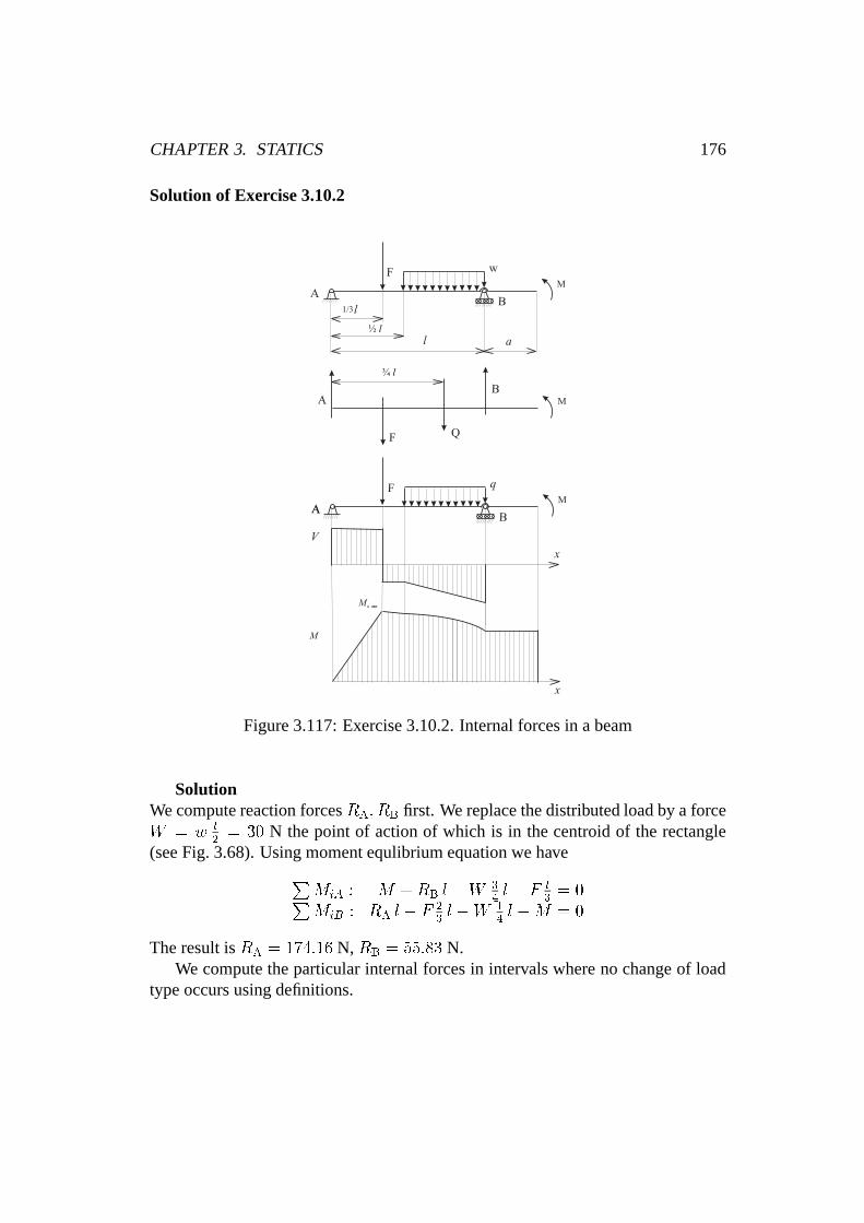
Figure 3.117: Exercise 3.10.2. Internal forces in a beam
SolutionWe compute reaction forcesRA; RB first. We replace the distributed load by a forceW = w l
2= 30 N the point of action of which is in the centroid of the rectangle
(see Fig. 3.68). Using moment equlibrium equation we havePMiA : M +RB l �W 3
4l � F l
3= 0P
MiB : RA l � F 23l �W 1
4l �M = 0
The result isRA = 174:16 N, RB = 55:83 N.We compute the particular internal forces in intervals where no change of load
type occurs using definitions.

CHAPTER 3. STATICS 177
Interval0 < x < l3:
N = 0V = RA = 174:16NMb = RA x = (174:16 x) Nm
Interval l3< x < l
2:
N = 0V = RA � F = �25:840NMb = RA x� (x� l
3)F = (�25; 84 x+ 40)Nm
Interval l2< x < l:
N = 0V = RA � F � w (x� l
2) = (4; 16� x) N
Mb = RA x� (x� l3)F � w (x� l
2)12(x� l
2)
Interval l < x < l + a:
N = 0V = RA � F � w l
2+RB = 0N
Mb = RA x� F (x� l3)� w l 1
2(x� 3
4l) +RB (x� l)
The plot of results is shown in Fig.3.68. You can see that maximum bending mo-mentMbmax is in position
x =l
3= 0:2 m
whereV = 0 occurs. Its value isMomax = 34:832 Nm.
Notice: See Matlab filebeam2D.m for numerical solution.

CHAPTER 3. STATICS 178
Solution of Exercise 3.11.2
r
kj,rj
M
Mkj
R
GS
ì
Figure 3.118: Exercise 3.11.2. Free-body diagram
Equation of equilibrium:M = S r +Mkj
The force in the spring:S = k x
The moment of friction:
Mkj = rj �kjR = rj �kj (S +G)
The momentM as a function ofx:
M = k x r + rj �jk (k x +G)
Mechanical work ofM :
W =
ZM d'
Geometry:x = r '; dx = r d'
Computation:
W =
ZM
dx
r=
hZ0
[rj �kjr
G + k (1 +rj �jkr
) x] dx
W =rj �jkr
Gh+1
2k (1 +
rj �kjr
) h2
Result:W = 15:3 Nm

CHAPTER 3. STATICS 179
Solution of Exercise 3.11.3
Z
M
Figure 3.119: Exercise 3.11.3. Free-body diagram
Moment:M = Z r tan(� + ')
The force in spring:Z = k x
The friction angle:' = arctan�k = 2:862Æ
Geometry:
tan� =x
r '; ' =
x
r tan�; d' =
1
r tan�dx
After substitution we have:
M = k x r tan(� + ')
Mechanical work ofM :
W =
ZM d' =
ZM
r tan�dx
W =
hZ0
k xtan(� + ')
tan�dx =
1
2k h2
tan(�+ ')
tan�
Result:W = 11:6 Nm

CHAPTER 3. STATICS 180
Solution of Exercise 3.11.4
k
G
P
h1
s0
s
s0
l0
l0
0
G
G
PS
h
P
S
î
î
Figure 3.120: Exercise 3.11.4. Free-body diagram
First we redraw the body into the current position and we sketch all relevant forces,namelyG;P; S. Mechanical work of the forceP is the summ of mechanical workW1 needed for lifting the body, and mechanical workW2 needed for stretching ofthe spring.
Mechanical workW1:
W1 =
h1Z0
G dh = Gh1 = 10 : 0; 2 = 2 Nm
Mechanical workW2:
W2 =
s1Zs0
S ds =
�1Z�0
k � d� =1
2k (�21 � �20)
where�; �0; �1 denote deformations of the spring in current, original, and endpositions.Geometry:
l0 + �
l0 + �0 � h=S
G
As S = k �,G = k �0 the following is valid
� =G l0
k (l0 � h)

CHAPTER 3. STATICS 181
and forh = h1 we have
�1 =G l0
k (l0 � h1)
W2 =1
2k (�21��20) =
G2
2 k
�l20
(l0 � h1)2� 1
�=
102
2 : 100
�0:32
(0:3� 0:2)2� 1
�= 4Nm
Mechanical workWP of the forceP :
WP =W1 +W2 = 6 Nm

CHAPTER 3. STATICS 182
Solution of Exercise 3.11.5
Sr
Fsf
N
h
S
G
Q
r
3r 3r
Q
3r
x
N1
N1
Ff1
Ff1
G
e
Figure 3.121: Exercise 3.11.5. Free-body diagram
Mechanical work of the forceS done along the pathh is
WS =
hZ0
S dx
First we have to express the magnitude of the forceS as a function ofx. We freethe system of bodies in the current position for the purpose. We suppose rolling ofthe cylinder without slipping on the ground.
Equations of equilibrium of the cylinder:
S � Fsf � Ff1 = 0N �G�N1 = 0
Ff1 r +N e� Fsf r = 0
Equation of equilibrium of the plate:
N1 x�Q 3 r = 0
Friction force:Ff1 = N1 �k
After substitution and some manipulations we have:
S = Q 3 r�2�k +
e
r
� 1
x+G
e
r

CHAPTER 3. STATICS 183
hence
WS =6 rRr
S dx = Q 3 r�2�k +
er
� 6 rRr
dxx+G �
r
6 rRr
dx
WS = Q 3 r�2�k +
�
r
�ln 6 + G � 5
WS = 500 : 3 : 0:1�2 : 0:3 + 0:01
0:1
�ln 6 + 300 : 0:01 : 5
WS = 203:13 Nm

CHAPTER 3. STATICS 184
Solution of Exercise 3.11.6
l
Pr
½ r
l1
C
N
Fsf
1 Q
CPN
Ff
P
x
x
l1
l
S
C
ϕ ϕ
Figure 3.122: Exercise 3.11.6. Free-body diagram
The cylinder will roll without slipping at the beginning of its motion due to themagnitude of�s given. Hence the equations of equilibrium of the cylinder are
P � Fsf = 0 ; N �Q = 0 ; Qr
2sin'� Fs r = 0
and
P =Q
2sin'
Simultaneously the condition for rolling have to be fulfilled:
Fs � N �s ; Fs � Q�sf
The maximum angle'1 follows from the maximum value ofFsf which is
Fsfmax = Q�sf =Q
2sin'1
2�sf = sin'1
For �s = 0:25, sin'1 = 0:5, '1 = 30Æ. It follows that in the first stage of motionthe coordinatex changes from0 to l1 = r '1.Geometry gives
x = r '; dx = r d'

CHAPTER 3. STATICS 185
Mechanical work of the forceP during the first stage of motion is
WP1 =l1R0
P dx = Qr
2
'1R0
sin' d'
WP1 = Q r2(1� cos'1) = 80 0:3
2(1� cos 30Æ) Nm
WP1 = 1:607 Nm
During the second stage of motion cylinder slips on the ground along the pathl1 ! ldue to forceP = Q�k magnitude of which is constant.
Mechanical work of the forceP during the second stage of motion is
WP2 = PlRl1
dx = Q�k (l � r '1)
WP2 = 80 : 0:25�1� 0:3 30�
180
�Nm
WP2 = 16:858 Nm
Mechanical work of the forceP along the whole pathl is
WP = WP1 +WP2 = (1:607 + 16:858) = 18:466 Nm

CHAPTER 3. STATICS 186
Solution of Exercise 3.12.2
F
ϕ
M = ?
p
Z
y
q
á
Figure 3.123: Exercise 3.12.2. Designation
The basic equation of pvw:
M Æ'+ F cos� Æp� F sin� Æq � Z Æy = 0
Geometry:p = konst:+ r cos'; Æp = �r sin' Æ'q = konst:+ r sin'; Æq = r cos' Æ'y = konst:+ r sin'; Æy = r cos' Æ'
After substitution we have
M Æ'� F cos� r sin' Æ'� F sin� r cos' Æ'� Z r cos' Æ' = 0
HenceM = r [F (cos� sin'+ sin� cos') + Z cos']
orM = r [F sin(� + ') + Z cos']
ResultM = 42:8 Nm
CHAPTER 3. STATICS 187
Solution of Exercise 3.12.3
ϕ
Z
z
5r
S
l
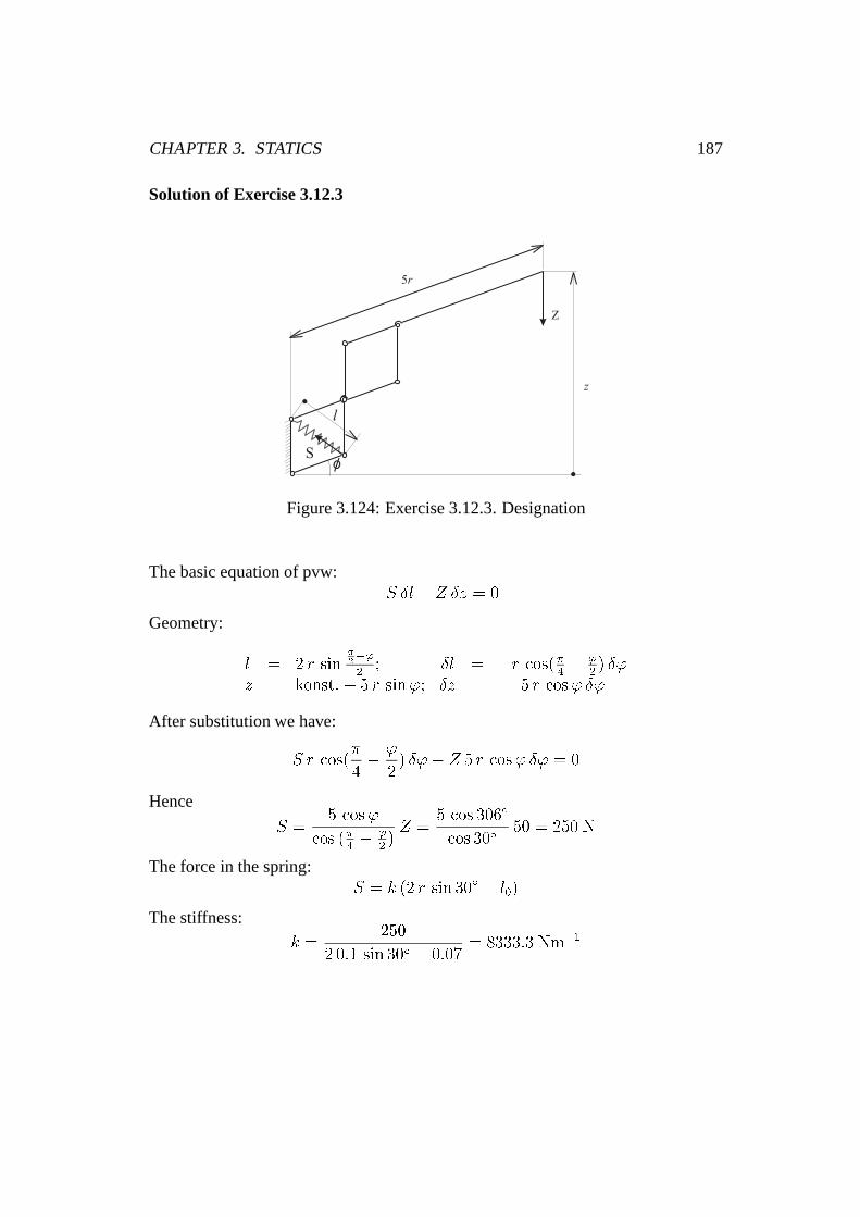
Figure 3.124: Exercise 3.12.3. Designation
The basic equation of pvw:�S Æl � Z Æz = 0
Geometry:
l = 2 r sin�2�'2; Æl = �r cos(�
4� '
2) Æ'
z = konst: + 5 r sin'; Æz = 5 r cos' Æ'
After substitution we have:
S r cos(�
4� '
2) Æ'� Z 5 r cos' Æ' = 0
Hence
S =5 cos'
cos (�4� '
2)Z =
5 cos 306Æ
cos 30Æ50 = 250 N
The force in the spring:S = k (2 r sin 30Æ � l0)
The stiffness:
k =250
2 0:1 sin 30Æ � 0:07= 8333:3 Nm�1

CHAPTER 3. STATICS 188
Solution of Exercise 3.12.4
S
r
1.2 r
ϕ
Z
zr
l
á
Figure 3.125: Exercise 3.12.4. Designation
The basic equation of pvw:�Z Æz + S Æl = 0
Geometry:
z = 1:2 r sin('� �); Æz = 1:2 r cos('� �) Æ'l = 2 r sin '
2; Æl = 2 r cos '
212Æ'
After substitution we have
S =Æz
ÆlZ =
l:2 r cos('� �) Æ'
2 r cos '
212Æ'
Z
Hence
S =1:2 cos('� �)
cos '
2
Z
S =1:2 cos 5Æ
cos 30Æ2500 = 3450:92 N
The force in the spring isS = k � = k 0:1
Result:k = 10S = 34509:2 Nm�1

BIBLIOGRAPHY 189
Solution of Exercise 3.12.5
Q
ϕr
l
l
r1 = 0
yM
ø
Figure 3.126: Exercise 3.12.5. Designation
The basic equation of pvw:
�QÆy +M Æ = 0
Geometry:
y = l2sin'; Æy = l
2cos Æ'
r = lp2� 2 l sin
�2�'2; Æ = l
rcos(�
4� '
2) Æ'
After substitution we have
�Q l
2cos' Æ'+M
l
rcos(
�
4� '
2) Æ' = 0
Result:
M =r
2
cos'
cos(�4� '
2)Q =
0:1
2
cos 30Æ
cos 30Æ5000 = 250 Nm
Bibliography
[1] P. F. Beer and E. R. Johnston Jr.Vector Mechanics for Engineers. Statics.McGraw-Hill, New York, 5th edition, 1988.
[2] David J. McGill and Wilton W. King.Engineering Mechanics: An Introductionto Statics and Dynamics.PWS Publishers, Boston, 1st edition, 1985.
[3] V. Stejskal, J. Brezina, and J. Knezu. Mechanika I.Rešené pˇríklady. Vydava-telstvíCVUT, Praha, 1st edition, 1999. (in Czech).