3122 ieee transactions on automatic...

3122 IEEE TRANSACTIONS ON AUTOMATIC CONTROL, VOL. 59, NO. 12, DECEMBER 2014

Finite Bisimulations for Switched Linear SystemsEbru Aydin Gol, Xuchu Ding, Mircea Lazar, and Calin Belta

Abstract—In this paper, we consider the problem of construct-ing a finite bisimulation quotient for a discrete-time switchedlinear system in a bounded subset of its state space. Given aset of observations over polytopic subsets of the state space anda switched linear system with stable subsystems, the proposedalgorithm generates the bisimulation quotient in a finite numberof steps with the aid of sublevel sets of a polyhedral Lyapunovfunction. Starting from a sublevel set that includes the origin in itsinterior, the proposed algorithm iteratively constructs the bisimu-lation quotient for the region bounded by any larger sublevel set.We show how this bisimulation quotient can be used for synthesisof switching laws and verification with respect to specificationsgiven as syntactically co-safe Linear Temporal Logic formulaeover the observed polytopic subsets.

Index Terms—Abstractions, formal methods, switched systems.

I. INTRODUCTION

IN recent years, there has been a trend to bridge the gapbetween control theory and formal methods. Control theory

allows for analysis and control of “complex” dynamical sys-tems with infinite state spaces, such as systems of controlleddifferential equations, against “simple” specifications, such asstability and reachability. In formal methods, “simple” systems,such as finite transition systems, are checked against “complex”(rich and expressive) specification languages, such as temporallogics. Recent studies show that certain classes of dynamicalsystems can be abstracted to finite transition systems. Appli-cations in robotics [1], multi-agent control systems [2], andbioinformatics [3] show that model checking and automatagames can be used to analyze and control systems with non-trivial dynamics from specifications given as temporal logicformulae.

In this paper, we focus on switched linear systems madeof stable subsystems, and show that a finite bisimulation ab-straction of the system can be efficiently constructed withinsome bounded subset of the state space. Since the bisimula-

Manuscript received February 13, 2013; revised December 8, 2013 andApril 19, 2014; accepted May 5, 2014. Date of publication August 28, 2014;date of current version November 18, 2014. This work was partially supportedby the NSF under grants CNS-0834260 and CNS-1035588 and by the ONRunder grant MURI N00014-09-1051 at Boston University, and by Veni grant10230 at Eindhoven University of Technology. Recommended by AssociateEditor G. J. Pappas.

E. Aydin Gol and C. Belta are with Boston University, Boston, MA 02215USA (e-mail: [email protected]; [email protected]).

X. Ding is with United Technologies Research Center, East Hartford,CT 06108 USA (e-mail: [email protected]).

M. Lazar is with Eindhoven University of Technology, 5612 AZ Eindhoven,The Netherlands (e-mail: [email protected]).

Color versions of one or more of the figures in this paper are available onlineat http://ieeexplore.ieee.org.

Digital Object Identifier 10.1109/TAC.2014.2351653

tion quotient preserves all properties that are expressible inframeworks as rich as µ-calculus, and implicitly ComputationTree Logic (CTL) and Linear Temporal Logic (LTL) (seee.g., [4]–[6]), it can be readily used for system verificationand controller synthesis against such specifications. We showhow our method can be used for both controller synthesis andverification from specifications given as arbitrary formulae of afragment of LTL, called syntactically co-safe LTL (scLTL) [7].For controller synthesis, we find the largest set of initial statesand switching sequences such that all system trajectories satisfya given formula. For verification, we find the largest set of initialstates such that all system trajectories satisfy the formula underarbitrary switching.

The concept of constructing a finite quotient of an infinitesystem has been widely studied, e.g., [8]–[12]. It is known thatfinite state bisimulation quotients exist only for specific classesof systems (e.g., timed automata [10] and controllable linearsystems [8]), and the well known bisimulation algorithm [4] ingeneral does not terminate [13]. For piecewise linear systems,guided refinement procedures were employed with the goal ofconstructing an over-approximating quotient that can be usedfor verification of universal properties [9], [13].

We propose to obtain a finite bisimulation quotient of thesystem by only considering the system behavior within a rele-vant state space that does not contain the origin, i.e., in betweentwo positively invariant compact sets that contain the origin.Our approach relies upon the existence of a common infinitynorm Lyapunov function, which is a necessary condition forstability under arbitrary switching [14]. We propose to partitionthe state space by using sublevel sets of the Lyapunov function.Such sublevel sets, which are polytopic, allow us to generatethe bisimulation quotient incrementally as the abstraction al-gorithm iterates, with no “holes” in the covered state space.Since we can obtain polytopic sublevel sets of any size fromthe Lyapunov function, the balance between the size of theabstracted state space and the amount of computation can beeasily adjusted and controlled. Starting from the observationthat the existence of the Lyapunov function renders the originasymptotically stable for the switched system, its trajectoriescan only spend a finite time in the region of interest. As aresult, we restrict our attention to LTL specifications that canbe satisfied in finite time, such as scLTL formulae.

The construction of finite abstractions of dynamical systemsby utilizing stability properties and Lyapunov functions wasstudied in [15], [16]. Approximately bisimilar finite abstrac-tions for continuous-time switched systems were constructedunder incremental stability assumptions in [15], where sublevelsets of a common Lyapunov function (or multiple Lyapunovfunctions with additional assumptions) were used. The ab-stract model was defined by quantizing the state space of

0018-9286 © 2014 IEEE. Personal use is permitted, but republication/redistribution requires IEEE permission.See http://www.ieee.org/publications_standards/publications/rights/index.html for more information.

AYDIN GOL et al.: FINITE BISIMULATIONS FOR SWITCHED LINEAR SYSTEMS 3123

the switched system, and sampling the trajectories originatingfrom the quantized state space. The approximate bisimulationrelation guarantees that the trajectories of the abstract modeland the original system are close to each other [17]. In [15],the accuracy of the abstraction was defined by the quantizationparameter and the Lyapunov function. The method developedin [15] is not limited to linear systems, however, the abstractionis approximate, and the case studies presented in [15] highlightthat a considerable accuracy requires a large abstract model.On the other hand, our method relies on efficient computationof one step controllable sets, hence suitable for linear systems.However, the resulting abstract model is exact in the sensethat it produces the same set of observations as the originalsystem. The authors of [15] relaxed the incremental stabilityassumption in their recent work on construction of approximatesimulations [18]. Another conceptually related work is [16],where n Lyapunov functions were used for the abstractionof n-dimensional continuous-time Morse-Smale systems (e.g.,hyperbolic linear systems) to timed automata. The abstractionproposed therein is weaker than bisimulation, but it can beused to verify safety properties. While both [16] and this workuse sublevel sets for abstraction, the main difference between[16] and this approach comes from the usage of polyhedralLyapunov functions, and therefore different classes of systemsfor which the methods apply. Our approach removes the needfor multiple orthogonal Lyapunov functions, and we arguethat it allows for a more tractable implementation since theabstraction of timed automata is expensive by itself [10], andpolytopic sublevel sets ensure that the abstraction algorithmrequires only basic operations with polytopic sets.

Preliminary versions of this work appeared in [19], [20]. In[19], we used polytopic sublevel sets to generate a bisimulationquotient for a discrete autonomous linear system, and in [20]we extended this approach to switched linear systems. Herewe expand these preliminary versions by including analysisof complexity, more technical details, e.g., the proofs of thetechnical results, and illustrative case studies. In addition, weshow how the proposed approach can be extended to piecewiselinear systems and polytopic difference inclusion systems.

The rest of the paper is organized as follows. We intro-duce preliminaries in Section II and formulate the problem inSection III. We present the algorithm to generate the bisim-ulation quotient in Section IV, and analyze the complexityassociated with it in Section V. We show in Section VI howthe resulting bisimulation quotient can be used to synthesizeswitching control laws and verify the system behavior againsttemporal logic formulae. We illustrate the findings of the paperwith examples in Section VII and summarize conclusions inSection VIII.

II. PRELIMINARIES

For a set S , int(S), |S|, and 2S stand for its interior, cardi-nality, and power set, respectively. For λ ∈ R and S ⊆ Rn, letλS := λx | x ∈ S. We use R, R+, Z, and Z+ to denote thesets of real numbers, non-negative reals, integer numbers, andnon-negative integers. For m, n ∈ Z+, we use Rn and Rm×n todenote the set of column vectors and matrices with n and m × n

real entries. For a vector v or a matrix A, we denote v⊤ or A⊤

as its transpose, respectively. For a vector x ∈ Rn, [x]i denotesthe i-th element of x and ∥x∥∞ = maxi=1,...,n |[x]i| denotesthe infinity norm of x, where | · | denotes the absolute value.For a matrix Z ∈ Rl×n, let ∥Z∥∞ := supx =0(∥Zx∥∞/∥x∥∞)denote its induced matrix infinity norm.

A n-dimensional polytope P (see, e.g., [21]) in Rn canbe described as the convex hull of at least n + 1 affinelyindependent points in Rn. Alternatively, P can be described asthe intersection of k, where k ≥ n + 1, closed half spaces, i.e.,there exist k ≥ n + 1 and HP ∈ Rk×n, hP ∈ Rk, such that

P = x ∈ Rn|HPx ≤ hP.

We assume polytopes in Rn are n-dimensional unlessnoted otherwise. The set of boundaries of a polytope P arecalled facets, denoted by f(P), which are themselves (n − 1)-dimensional polytopes. A semi-linear set (also called a polyhe-dron in literature) in Rn is defined as finite unions, intersectionsand complements of sets x ∈ Rn | a⊤x ∼ b,∼∈ =, <, forsome a ∈ Rn and b ∈ R. Note that a convex and bounded semi-linear set is equivalent to a polytope with some (or none) of itsfacets removed.

A. Transition Systems and Bisimulations

Definition 2.1: A transition system (TS) is a tuple T =(Q,Σ,→,Π, h), where

• Q is a (possibly infinite) set of states;• Σ is a set of inputs;• →⊆ Q × Σ× Q is a set of transitions;• Π is a finite set of observations; and• h : Q −→ 2Π is an observation map.

We denote xσ→ x′ if (x,σ, x′) ∈→. We assume T to be non-

blocking, i.e., for each x ∈ Q, there exists x′ ∈ Q and σ ∈ Σsuch that x

σ→ x′. An input word is defined as an infinitesequence σ = σ0σ1 . . . where σk ∈ Σ for all k ∈ Z+. A tra-jectory of T produced by an input word σ = σ0σ1 . . . andoriginating at state x0 is an infinite sequence x = x0x1 . . .where xk

σk→ xk+1 for all k ∈ Z+. A trajectory x generates aword o = o0o1 . . ., where ok ⊆ Π is the set of observations ofstate xk and defined as ok := h(xk) for all k ∈ Z+.

The TS T is finite if |Q| < ∞ and |Σ| < ∞, otherwise Tis infinite. Moreover, T is deterministic if x

σ→ x′ implies thatthere does not exist x′′ = x′ such that x

σ→ x′′; otherwise, T iscalled non-deterministic. Given a set Q ⊆ Q, we define the setof states PreT (Q,σ) that reach Q in one step when input σ isapplied as

Preτ (Q,σ) := x ∈ Q| ∃x′ ∈ Q, xσ→ x′. (1)

States of a TS can be related by a relation ∼⊆ Q × Q. Forconvenience of notation, we denote x ∼ x′ if (x, x′) ∈∼.

Definition 2.2: We say that a relation ∼ is observation pre-serving if for any x, x′ ∈ Q, x ∼ x′ implies that h(x) = h(x′).

For an observation preserving relation ∼, the subset Q ⊆Q is called an equivalence class if x, x′ ∈ Q ⇔ x ∼ x′. Wedenote by Q/∼ the set labeling all equivalence classes anddefine a map eq : Q/∼ 0→ 2Q such that eq(X) is the set of statesin the equivalence class Q ∈ Q/∼ labeled by X .


Definition 2.3: A finite partition P of a set S is a finitecollection of sets P := Pii∈I , such that ∪i∈IPi = S and Pi ∩Pj = ∅ if i = j. A finite refinement of P is a finite partition P ′

of S such that for each Pi ∈ P ′, there exists Pj ∈ P such thatPi ⊆ Pj .

A partition naturally induces a relation, and an observationpreserving relation induces a quotient TS. One can immediatelyverify that a refinement of an observation preserving partitionis also observation preserving.

Definition 2.4: An observation preserving relation ∼ of aTS T = (Q,Σ,→,Π, h) induces a quotient transition systemT /∼ = (Q/∼,Σ,→∼,Π, h∼), where Q/∼ is the set labelingall equivalence classes. The transitions of T /∼ are defined asX

σ→∼ Y if and only if there exists x ∈ eq(X) and x′ ∈ eq(Y )such that x

σ→ x′. The observation map is defined as h∼(X) :=h(x), where x ∈ eq(X).

Definition 2.5: Given a TS T =(Q,Σ,→,Π, h), a relation ∼is a bisimulation relation of T if (1) ∼ is observation preserv-ing; and (2) for any x1, x2∈Q,σ∈Σ, if x1∼x2 and x1

σ→x′1,

then there exists x′2 ∈ Q such that x2

σ→ x′2 and x′

1 ∼ x′2.

If ∼ is a bisimulation, then the quotient transition system T/∼is called a bisimulation quotient of T . In this case, T and T /∼are said to be bisimilar. Bisimulation is a very strong equiva-lence relation between systems. In fact, it preserves propertiesexpressed in temporal logics such as LTL, CTL and µ-calculus[4]–[6]. As such, it is used as an important tool to reduce thecomplexity of system verification or controller synthesis, sincethe bisimulation quotient (which may be finite) can be verifiedor used for controller synthesis instead of the original system.

B. Polyhedral Lyapunov Functions

Consider an autonomous discrete-time system,

xk+1 = Φ(xk), k ∈ Z+ (2)

where xk ∈ Rn is the state at the discrete-time instant k andΦ : Rn 0→ Rn is an arbitrary map with Φ(0) = 0. Given a statex ∈ Rn, x′ := Φ(x) is called a successor state of x.

Definition 2.6: Let λ ∈ [0, 1]. We call a set P ⊆ Rn

λ-contractive (shortly, contractive) if for all x ∈ P it holds thatΦ(x) ∈ λP . For λ = 1, we call P a positively invariant set.

A function α : R+ → R+ belongs to class K∞ if it is contin-uous, strictly increasing, α(0) = 0 and lims→∞ α(s) = ∞.

Theorem 2.1: Let X be a positively invariant set for (2) with0 ∈ int(X ). Furthermore, let α1,α2 ∈ K∞, ρ ∈ (0, 1) and V :Rn 0→ R+ such that:

α1(∥x∥) ≤ V (x) ≤α2(∥x∥), ∀x ∈ X (3)

V (Φ(x)) ≤ ρV (x), ∀x ∈ X . (4)

Then system (2) is asymptotically stable in X .The proof of Theorem 2.1 can be found in [22], [23].Definition 2.7: A function V : Rn 0→ R+ is called a

Lyapunov function (LF) in X if it satisfies (3) and (4). IfX = Rn, then V is called a global Lyapunov function.

The parameter ρ is called the contraction rate of V . For anyΓ>0, PΓ :=x ∈ Rn | V (x)≤Γ is called a sublevel set of V .

For the remainder of this paper we consider LFs definedusing the infinity norm, i.e.,

V (x) = ∥Lx∥∞, L ∈ Rl×n, l ≥ n, l ∈ Z+ (5)

where L has full-column rank. Notice that infinity normLyapunov functions are a particular type of polyhedralLyapunov functions. We opted for this type of function to sim-plify the exposition but in fact, the proposed abstraction methodapplies to general polyhedral Lyapunov functions defined byMinkowski (gauge) functions of polytopes in Rn with the originin their interior.

Proposition 2.1: Suppose that L ∈ Rl×n has full-columnrank and V as defined in (5) is a global LF for system (2) withcontraction rate ρ ∈ (0, 1). Then for all Γ > 0 it holds that PΓ isa polytope and 0 ∈ int(PΓ). Moreover, if Φ(x) = Ax for someA ∈ Rn×n, then for all Γ > 0 it holds that PΓ is a ρ-contractivepolytope for (2).

The proof of the above result is a straightforward applicationof results in [24], [25].

In this paper, we will consider switched systems that arestable under arbitrary switching. In this case, the dynamicscorresponding to (2) becomes a difference inclusion, i.e., x′ ∈Φ(x), Φ(x) := Ax | A ∈ A for some set A ⊆ Rn×n. It hasbeen shown in [24], [25], that all the above definitions (invariantset, Lyapunov function) and results apply directly to differenceinclusions in the absolute sense, i.e., given x, the correspondingconditions must hold for all x′ ∈ Φ(x).

III. PROBLEM FORMULATION

In this paper, we consider discrete-time switched linearsystems, i.e.,

xk+1 = Aσ(k)xk, σ(k) ∈ Σ, k ∈ Z+ (6)

where σ : Z+ → Σ is a switching sequence that selects theactive subsystem from a finite index set Σ and Ai ∈ Rn×n isa strictly stable (i.e., Schur) matrix for all i ∈ Σ. We assumethat a common polyhedral Lyapunov function (LF) of the form(5) with contraction rate ρ ∈ (0, 1) is known for system (6).The algorithm proposed in [25] is employed to construct such afunction with a desired contraction rate.

Let X be a polytope X := x | ∥Lx∥∞ ≤ ΓX and D bea polytope D := x | ∥Lx∥∞ ≤ ΓD, where L correspondsto the polyhedral LF (5) of system (6) and we assume that0 < ΓD < ΓX . Note that D ⊂ X and 0 ∈ int(D) ⊂ int(X ). Wecall X the working set and D the target set. We are interestedin synthesis of control strategies and verification of the systembehavior within X with respect to polytopic regions in the statespace, until the target set D is reached (since D is positivelyinvariant, the system trajectory will be confined within D afterD is reached).

We assume that there exists a set R of polytopes indexed bya finite set R, i.e., R := Rii∈R, where Ri ⊆ X \ D for alli ∈ R, and Ri ∩ Rj = ∅ for any i = j. The set R represents re-gions of interest in the relevant state space, and the polytopes inR are considered as observations of (6). Therefore, a trajectoryof (6) x0x1 . . . produces an infinite sequence of observations


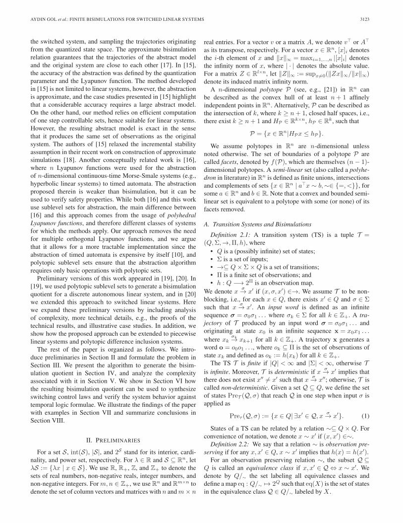
Fig. 1. An example in R2 of the working set X , the target set D (in brown),a set of observational relevant polytopes R = R1, R2, R3 (in transparentgreen), sublevel sets with N = 11 and one slice S6 (in purple).

o0o1 . . ., such that oi is the index of the polytope in R visitedby state xi, or oi = ∅ if xi is in none of the polytopes.

Example 3.1: Consider a system as in (6), Σ = 1, 2,

A1 =

(−0.65 0.32−0.42 −0.92

)and A2 =

(0.65 0.32−0.42 −0.92

). The

algorithm proposed in [25] is employed to construct a globalpolyhedral LF of the form (5), where

L =

(−0.0625 0.6815 0.9947 0.9947

1 1 −0.6868 −0.0678

)⊤

and ρ = 0.94. We chose ΓX = 10 and ΓD = 5.063. (see Fig. 1for polytopes X , D, and a set of polytopes R.) !

The semantics of the system can be formalized through anembedding of (6) into a transition system, as follows.

Definition 3.1: Let X , D, and R = Rii∈R be given. Theembedding transition system for (6) is a transition system Te =(Qe,Σ,→e,Π, he) where

• Qe := X ;• Σ is the same as the index set given in (6);• 1) If x ∈ X \ D, then x

σ→e x′ if and only if x′ = Aσx,i.e., x′ is the state at the next time-step after applyingthe dynamics of (6) at x when subsystem σ is active;

2) If x ∈ D, xσ→e x for all σ ∈ Σ (since the target set D

is already reached, we consider the behavior of thesystem thereafter no longer relevant);

• Π = R ∪ ΠD, i.e., the set of observations is the set oflabels of regions, plus the label ΠD for D;

• 1) he(x) := i if and only if x ∈ Ri;2) he(x) := ∅ if and only if x ∈ X \ (D ∪

⋃i∈R Ri);

3) he(x) := ΠD if and only if x ∈ D.

Note that Te is deterministic and it has an infinite numberof states. Moreover, Te exactly captures the system dynamicsunder (6) in the relevant state space X \ D, since a transitionof Te naturally corresponds to the evolution of the discrete-timesystem in one time-step. Indeed, within X \ D, the trajectoryof Te produced by an input word σ from a state x ∈ X \ D isexactly the same as the trajectory of system (6) from x underthe switching sequence σ.

We now formulate the main problem considered in this paper.

Problem 3.1: Let a system (6) with a polyhedral Lyapunovfunction of the form (5), sets X , D, and Rii∈R be given.Compute a finite observation preserving partition P suchthat its induced relation ∼ is a bisimulation of the embeddingtransition system Te, and obtain the corresponding bisimulationquotient Te/∼.

Remark 3.1: The above assumptions on the sets X , D, andRii∈R are made for simplicity of presentation. The problemformulation and the approach described in the rest of the papercan be easily extended to arbitrary positively invariant sets Xand D with D ⊆ X , i.e., not obtained as the sublevel sets of(5), by considering the largest sublevel set that is included inD and the smallest sublevel set that includes X (ΓD and ΓXcan be made arbitrarily small and arbitrary large, respectively,so as to capture any compact subset of Rn). Also, the set ofpolytopes of interest Rii∈R can be relaxed to a finite set oflinear predicates in x as defined in [26].

IV. BISIMULATION QUOTIENT

Starting from a polyhedral Lyapunov function V (x)=∥Lx∥∞with a contraction rate ρ∈(0, 1) as described in Section II-B forsystem (6), we first generate a sequence of polytopic sublevelsets of the form PΓ := x ∈ Rn | ∥Lx∥∞ ≤ Γ as follows.Recall that X = PΓX and D = PΓD for some 0 < ΓD < ΓX .We define a finite sequence Γ := Γ0, . . . ,ΓN , where

Γi+1 = ρ−1Γi, i = 0, . . . , N − 2 (7)

Γ0 := ΓD, ΓN := ΓX , and

N := arg minN

ρ−NΓ0|ρ−NΓ0 ≥ ΓX . (8)

This choice of N guarantees that PΓN−1 is the largest sublevelset defined via (7) that is a subset of X . Since ΓN is exactly ΓX ,PΓN is exactly X .

The sequence Γ generates a sequence of sublevel sets PΓ :=PΓ0 , . . . ,PΓN . From the definition of the sublevel sets and Γ,we have that

PΓ0 ⊂ . . . ⊂ PΓN . (9)

Next, we define a slice of the state space as follows:

Si := PΓi \ PΓi−1 , i = 1, . . . , N. (10)

For convenience, we also denote S0 := PΓ0 (although S0 is nota slice in between two sublevel sets). We immediately see thatthe sets Sii=0,...,N form a partition of X . Note that the slicesare bounded semi-linear sets (see Section II).

Example 4.1 (Example 3.1 Continued): Consider the systemgiven in Example 3.1. The sequence Γ is computed from ΓX ,ΓD, and ρ as described above, which resulted in N = 11.The polytopic sublevel sets PΓ := PΓ0 , . . . ,PΓ11 are shownin Fig. 1. !

Proposition 4.1: Assume that the set of slices Sii=0,...,N

is obtained from a sequence Γ satisfying (7). Given a state x inthe i-th slice, i.e., x ∈ Si, where 1 ≤ i ≤ N , its successor state(x′ = Aσx, σ ∈ Σ) satisfies x′ ∈ Sj for some j < i.


Proof: From Proposition 2.1, we have that PΓi areρ-contractive. By the definition of a ρ-contractive set(Definition 2.6), we have that x′ = Aσx ∈ ρPΓi = x ∈Rn | ∥Lx∥∞ ≤ ρΓi for all σ ∈ Σ. From (7), we have ρΓi =Γi−1. Therefore PΓi−1 = x ∈ Rn | ∥Lx∥∞ ≤ Γi−1 impliesthat PΓi−1 = x ∈ Rn | ∥Lx∥∞ ≤ ρΓi and hence PΓi−1 =ρPΓi and x′ ∈ PΓi−1 . From the definition of slices (10), x′ ∈Sj for some j < i. !

The state space of Te (which is the working set X ) can benaturally partitioned as

PX :=

Rii∈R, X \

(D ∪

⋃

i∈R

Ri

), D

. (11)

The relation induced from partition PX is observation pre-serving (see Section II-A).

The proposed abstraction algorithm computes the bisimula-tion quotient by iteratively refining an observation preservingpartition with respect to one step controllable sets. We first ex-plain two procedures, ComputePre and RefineUpdate, whichare used by the main abstraction algorithm. The procedureComputePre(P,σ) takes as input P , which is a bounded semi-linear set (e.g., a slice), and σ ∈ Σ, which is the switching input,and returns the set PreTe(P,σ). In general, if P is a semi-linear set, then PreTe(P,σ) is also a semi-linear set and it canbe computed via quantifier elimination [27]. In particular, thecomputation of PreTe for a bounded semi-linear set P falls intoone of the following cases:

(i) If P is a polytope, then PreTe(P,σ) is computed as:

Preτe(P,σ) = x ∈ Rn|HPAσx ≤ hP (12)

which is a possibly degenerate polytope in Rn. Note that(12) applies to a polytope P of any dimension;

(ii) If P is a union of polytopes, one can use a standardconvex decomposition method to decompose P into aset of polytopes Pii∈I (see, e.g., [21]), and computePreTe(P,σ) as ∪i∈IPreTe(Pi,σ) using (12);

(iii) If P is a convex and bounded semi-linear set, thenP =P\∪i∈IFi for some polytope P and its facet Fi∈f(P). Since Te is deterministic, we have PreTe(P,σ)=PreTe(P,σ)\PreTe(∪i∈IFi,σ), where the second termcan be computed as described in case (ii);

(iv) If P is a general (non-convex) bounded semi-linearset, then again it can be decomposed into con-vex and bounded semi-linear sets P = ∪i∈I Pi. ThenPreTe(P,σ) = ∪i∈IPre(Pi,σ), and each Pre(Pi,σ)can be computed as described in case (iii).

As summarized above, we see that ComputePre(P,σ) canalways be implemented by convex decompositions and repeatedapplications of (12), and thus ComputePre(P,σ) only requiresbasic operations with polytopic sets.

The procedure RefineUpdate(P, T , P ,σ, q) (outlined inAlgorithm 1) refines a partition P with respect to set P , whereP = ComputePre(eq(q),σ). It then updates T . If P consistsof only bounded semi-linear sets and P is a semi-linear set,then the resulting refinement P+ consists of only boundedsemi-linear sets. This fact allows us to compute PreTe(P,σ)

with ComputePre(P ,σ) only taking bounded semi-linear setsas inputs.

Algorithm 1 [P+, T +] = RefineUpdate(P, T , P ,σ, q)

Input: A TS T = (Q,Σ,→,Π, h), a partition P whereeq(q′)∈P for all q′ ∈Q, and P =ComputePre(eq(q),σ)for some q ∈ Q, σ ∈ Σ.

Output: P+ is a finite refinement of P with respect to P ,T + is a TS updated from T .

1: Set P+ = P and T + = T .2: for all q′ ∈ Q+ such that eq(q′) ∩ P = ∅ do3: Replace q′ in Q+ by q1, q2 and set eq(q1)=eq(q′)∩

P , eq(q2) = eq(q′) \ P .4: Replace eq(q′) in P+ by eq(q1), eq(q2).5: Replace each (q′,σ′, q′′) ∈→+ by (qi,σ′, q′′)i=1,2.6: Add transition (q1,σ, q) to →+.7: end for

We now present the abstraction algorithm (see Algorithm 2)that computes the bisimulation quotient. The main idea isto start with PX (11), refine the partition according toSii=0,...,N so that it is a refinement to both PX , andSii=0,...,N , and then iteratively refine using the Pre operator(1) until the bisimulation quotient is obtained. Starting withPX is necessary so that the partition is observation preserving.The second step guarantees that each element in the partitionis included in a slice. The third step allows us to ensure that atiteration i of the algorithm, the bisimulation quotient for stateswithin PΓi is completed.

Algorithm 2 Abstraction algorithm

Input: System dynamics (6), polyhedral LF V (x) = ∥Lx∥∞with a contractive rate ρ, sets X , D, and Rii∈R.

Output: Bisimulation quotient Te/∼ of the embedding tran-sition system Te and the corresponding observation preserving partition P .

1: Obtain PX as in (11).2: Generate the sequence of sublevel sets PΓ = PΓ0 , . . . ,

PΓN and slices S0, . . . ,SN as defined in (10).3: Set P0 = P1 ∩ P2 | P1 ∈ PX , P2 ∈ Sii=0,...,N , P1 ∩

P2 = ∅.4: Initialize Te/∼0 by setting Qe/∼0 as the set labeling P0.

Set transitions only for the state qD ∈ Qe/∼0 whereeq(qD) = S0 = D with qD

σ→∼0 qD for all σ ∈ Σ.5: for each i = 0, . . . , N − 1 do6: Set Te/∼i+1 = Te/∼i and Pi+1 = Pi.7: for each q ∈ Qe/∼i where eq(q) ⊆ Si do8: for each σ ∈ Σ do9: Find P = ComputePre(eq(q),σ).

10: Set [Pi+1, Te/∼i+1 ] = RefineUpdate

(Pi+1, Te/∼i+1 , P ,σ, q).11: end for12: end for13: end for14: Return Te/∼N and PN .


Fig. 2. The observed regions are shown in transparent green in (a) and (b). (a) At the end of the third iteration (i = 2), the bisimulation quotient for stateswithin PΓ3 is completed, which are shown in red PΓ2 ) and purple (S3). (b) In the forth iteration, the states within PΓ11 \ PΓ3 are partitioned according toPreTe (P,σ), P ∈ S3. S3 is shown in purple; PreTe (S3, 1) and PreTe (S3, 2) are shown in light and dark blue. (c) At the last iteration where i = 10, thealgorithm is completed. The state space covered by the bisimulation quotient is shown in red, covering all of X .

The correctness of Algorithm 2 will be shown by an inductiveargument. Given a sublevel set PΓi and a partition Pi asobtained in Algorithm 2, we define Pi as

Pi := P ∈ Pi|P ⊆ PΓi. (13)

From Algorithm 2, we see that P0 partitions all the slices, andsince Pi is a finite refinement of P0, we can directly see thatPi is a partition of PΓi . Let us define an embedding transitionsystem Te(i) as a subset of Te with set of states x ∈ Qe | x ∈PΓi and let us state the following result.

Proposition 4.2: At the completion of the i-th iteration (ofthe outer loop) of Algorithm 2 (where Pi+1 is obtained), if ∼i

induced by Pi as defined in (13) is a bisimulation of Te(i), then∼i+1 induced by Pi+1 is a bisimulation of Te(i + 1).

Proof: We show that at the end of i-th iteration, eachtransition originating at a state q ∈ Qe/∼i+1 with eq(q)⊆PΓi+1

satisfies the bisimulation requirement (Definition 2.5). ByProposition 4.1, for each x ∈ Si+1 and σ∈Σ, x′=Aσx must bein a slice with a lower index and thus x′ ∈Te(i). Let x∈eq(q)∈Pi. If x′ ∈Si, then we have x∈ P =ComputePre(eq(q′),σ)(from step 9 of Algorithm 2) for some q′ ∈Qe/∼i . TheRefineUpdate procedure replaces eq(q) with eq(q1)=eq(q)∩P and eq(q2)=eq(q) \ P , and updates Te/∼i+1 . We note fromthe definition of Pre operator (1) that for any x ∈ eq(q1), x′=Aσx∈eq(q′), thus for any x1, x2∈eq(q1), x1∼x2, Aσx1∼Aσx2. Moreover, the same argument holds for any subset ofeq(q1). Therefore, the transitions given in steps 5 and 6 ofAlgorithm 1 satisfy the bisimulation requirement. On the otherhand, if x′ ∈Si, then x′ ∈ Sj for some j <i and x is alreadyin a set eq(q), where q

σ→∼i+1 q′ for some q′ satisfying thebisimulation requirement. Therefore, step 9 of Algorithm 2provides exactly the transitions needed for all states in Si+1 andthus, ∼i+1 induced by Pi+1 is a bisimulation of Te(i+1). !

Theorem 4.1: Algorithm 2 returns a solution to Problem 3.1.Proof: From Algorithm 1, we have that Pi is a refinement

of PX for any i = 0, . . . , N . Therefore, PN and its inducedrelation ∼N are observation preserving.

At step 4 of Algorithm 2, we set qσ→e Q∼0q, ∀σ ∈ Σ where

eq(q) = D. From the definition of Te, we see that since D isthe only state, ∼0 induced by P0 is a bisimulation of Te(0).

Using Proposition 4.2 and induction, at iteration N − 1, wehave that ∼N induced by PN is a bisimulation of Te(N). Notethat PN is exactly PN , PΓN is exactly X and Te(N) is exactlyTe. Therefore ∼N induced by PN is a bisimulation of Te. !

At each iteration i, the number of updated sets is finite as thepartition Pi and the set of inputs Σ are finite, and therefore, wehave:

Corollary 4.1: A solution to Problem 3.1 can be generated ina finite number of steps, which is determined by the contractionrate of the Lyapunov function.

Example 4.2 (Example 4.1 Continued): Algorithm 2 is ap-plied on the same setting as in Example 4.1 to compute thebisimulation quotient. P3 and P11 are shown in Fig. 2.

A. Extensions

Although the focus of the paper is on switched linear systemswith polyhedral Lyapunov functions, the presented approachcan also be applied to other classes of discrete-time systemswith different Lyapunov functions, if

1) the sublevel sets of the Lyapunov function are semi-linearsets,

2) the pre-image of a bounded semi-linear set is computableand is also a semi-linear set, and

3) the dynamical system has a finite set of controls.The first condition guarantees that the slices (see (10)) are

semi-linear sets, and therefore the initial partition is composedof semi-linear sets. The second condition allows us to computepre-images throughout the algorithm. Finally the last conditionis necessary since the pre-images of the partition elements arecomputed for each control input (line 8 of Algorithm 2).

For example, consider discrete-time piecewise linear systemsdescribed by

xk+1 = Aσxk, xk ∈ Xσ,σ ∈ Σ, k ∈ Z+ (14)

where Σ is a finite index set of modes (different dynamics),Ppwl = Xσσ∈Σ is a partition of X and each Xσ is a semi-linear set. Under certain conditions, a Lyapunov function withpiecewise polytopic sublevel sets for system (14) exists [28].System (14) with a piecewise polyhedral Lyapunov functionsatisfies the properties given above. The extension to such


systems requires to refine the initial partition P0 according toPpwl. Then, the proposed algorithms can be used to constructa quotient transition system Te/∼. In this case, in step 2 ofAlgorithm 1 it is sufficient to refine a state q′ only if eq(q′) ⊂Xσ since only mode σ can be active in eq(q′). By eliminatingsome of the transitions of Te/∼ according to Ppwl, i.e., q σ→∼ q′

only if eq(q) ⊆ Xσ, we obtain a bisimulation quotient T pwle /∼

for the corresponding embedding transition system. This exten-sion is illustrated by an example in Section VII.

V. COMPLEXITY

Our algorithm involves computations of pre-images ofbounded semi-linear sets through linear dynamics, intersectionsand set differences for semi-linear sets at each iteration. Thenumber of operations performed, and hence the complexityof the algorithm, scale linearly with the size of the resultingpartition |PN |. Therefore, we derive an upper bound on |PN |with respect to the number of slices, observations and controls.

Let si be the number of sets in partition PN that are includedin slice Si, i.e.,

si := |P ∈ PN |P ⊆ Si|.

Similarly, s0i denotes the number of sets in the initial partition

P0 that are included in slice Si. In the subsequent analysis, r isused to denote the number of observations within X \ D (r =|R| + 1), and e is used to denote the number of input symbols(e = |Σ|).

Lemma 5.1: The number of sets in the resulting partition PN

that are included in slice i ≥ 1, si, is less than or equal to

si = r

(i−1∑

k=0

sk

)e

. (15)

Proof: A set P ∈ P0 with P ⊆ Si is partitioned only ifthere exists σ ∈ Σ and P ′ ∈ Sj for some j < i such that P ∩Pre(P ′,σ) = ∅ and P \ Pre(P ′,σ) =∅ (step 2 of Algorithm 1).Therefore,

(a) for any two states q1, q2 ∈ Qe/∼ with eq(q1), eq(q2) ⊂Si if h(q1) = h(q2), there exists σ ∈ Σ such that q1

σ→∼q′1, q2

σ→∼ q′2, and q′1 = q′2.From Proposition 4.1 and the bisimulation requirement

(Definition 2.5), we have that(b) for each q ∈ Qe/∼ with eq(q) ⊆ Si and for each σ ∈ Σ,

there exists a state q′ with eq(q′) ⊆ Sj for some j < i

such that qσ→∼ q′.

Given properties (a) and (b), the number of sets obtainedfrom partitioning a set P ∈ P0 with P ⊆ Si is bounded by thenumber of permutations of size e, with unrestricted repetitions,taken from a set of size

∑i−1k=0 sk.

The given bound is obtained by observing that s0i ≤ r for

all i = 1, . . . , N , since the initial partition P0 is obtained byrefining the coarsest observation preserving partition PX (see(11)) according to slice partition. !

The bound is computed through a combinatorial perspectiveby utilizing the contractive property of the system. Even though

Fig. 3. Comparison of the number of elements in a slice, si, and the corre-sponding bound, si (15).

the bound is attainable, the underlying dynamics is not con-sidered explicitly. Therefore, in many cases the bound is notattained, for example see Example 5.1.

Remark 5.1: PN is the coarsest refinement of P0 satis-fying the bisimulation requirement. This claim follows fromstatement-(a) of the proof of Lemma 5.1, and can easily beproven by an inductive argument on the partitions of the sub-level sets, i.e., Pi as defined in (13).

Example 5.1 (Example 4.2 Continued): The number of setsin partition P11 according to slice numbers and the correspond-ing bounds computed as in (15) are shown in Fig. 3. !

By using Lemma 5.1, we derive a bound on the number ofsets in PN that are included in sublevel set PΓi in closed form,i.e., the new bound depends only on sublevel set number i, thesize of the control set e and the number of observations r.

Theorem 5.1: Let pi = |P | P ∈ PN , P ⊆ PΓi| for all i =0, . . . , N . Then p0 = 1 and

pi ≤ (r + 1)∑i−1

j=0ej

, i = 1, . . . , N. (16)

Proof: As PΓ0 is not partitioned, the claim holds for i =0, i.e., p0 = 1. We prove the claim for i ≥ 1 by induction. Thedefinitions of pi, si, and si imply that

pi+1 = pi + si+1 ≤ pi + si+1.

From (15) s1 = r, and hence the claim holds for i = 1 as p1 ≤1 + r. Assume that inequality (16) holds for pk for some k ≥ 1.By Lemma 5.1, we have that sk+1 = rpe

k. Therefore

pk+1 ≤ pk + rpek < (r + 1)pe

k.

Using the inductive hypothesis on pk, the left hand side can berewritten as

pk+1 < (r + 1)

((r + 1)

∑k−1

j=0ej)e

pk+1 < (r + 1)

((r + 1)

∑k

j=1ej)

pk+1 < (r + 1)∑k

j=0ej

.

Thus, inequality (16) holds for pk+1, and by induction weconclude that (16) holds for all i = 1, . . . , N . !


The size, pN , of the resulting partition of the working set Xis double exponential with N when e > 1 (switched systems).Therefore when e > 1 the number of Pre operations performed,pN−1, is double exponential with N − 1. It is easy to verifyfrom (16) that the bound is exponential with N for linear sys-tems, i.e., e = 1. Note that the derived bound is an upper boundfor the worst case, i.e., when si = si for all i = 0, . . . , N .

Remark 5.2: The computational complexity increases withthe number of sublevel sets, N , which is computed from theworking set X , the target set D, and the contraction rate ρof the Lyapunov function (see (8)). Therefore, the amount ofcomputation can be adjusted by the choice of the working setX and the target set D for a given Lyapunov function. Forexample, the computation time can be decreased by choosing Das the largest sublevel set that does not intersect with the regionsof observations. In addition, using a Lyapunov function with aminimal contraction rate can decrease the computation time.Computation of such Lyapunov functions are out of the scopeof this paper, but for example, minimization of the contractionrate is possible via the algorithm presented in [28].

VI. TEMPORAL LOGIC SYNTHESIS AND VERIFICATION

After we obtain a bisimulation quotient for system (6), wecan solve verification and controller synthesis problems fromtemporal logic specifications such as CTL∗, CTL, and LTL.The asymptotic stability assumption implies that all trajectoriesof (6) sink in D. For this reason, we will focus on the syntacti-cally co-safe fragment of LTL, which includes all specificationsof LTL where satisfactions of trajectories can be determined bya finite prefix. Since we are interested in the behavior of (6) untilD is reached, scLTL is a sufficiently rich specification language.

A detailed description of the syntax and semantics of scLTLis beyond the scope of this paper and can be found in, forexample, [7], [29]. Roughly, an scLTL formula is built up froma set of atomic propositions Π, standard Boolean operators ¬(negation), ∨ (disjunction), ∧ (conjunction), ⇒ (implication)and temporal operators X (next), U (until), and F (eventually).1

The semantics of scLTL formulae is given over infinite wordso = o0o1 . . ., where oi ∈ 2Π for all i. We write o |= φ if theword o satisfies the scLTL formula φ. We say a trajectory qof a transition system T satisfies scLTL formula φ, if the wordgenerated by q (see Definition 2.1) satisfies φ.

Example 6.1: Again, consider the setting in Example 3.1with R = Rii=1,2,3. We now consider a specification inscLTL over R1, R2, R3,ΠD. For example, the specification“A system trajectory never visits R2 and eventually visits R1.Moreover, if it visits R3 then it must not visit R1 at the next timestep” can be translated to a scLTL formula:

φ := (¬R2 ∪ΠD) ∧ FR1 ∧ ((R3 ⇒ X¬R1) ∪ΠD). (17)

A. Synthesis of Switching Strategies

In this section, we assume that we can choose the dynamicsAσ , σ ∈ Σ to be applied at each step k. Our goal is to find

1The difference between LTL and scLTL is the lack of globally operatorin scLTL. Moreover, the negation can only be used in conjunction with thepropositions in a scLTL formula.

the largest set of initial states and a switching sequence (i.e.,a sequence of elements from Σ to be applied at each step) foreach initial state such that all the corresponding trajectories ofsystem (6) satisfy a temporal logic specification. As a switchedsystem is deterministic, it produces a unique trajectory fora given initial state and a switching sequence. Formally, weconsider the following problem:

Problem 6.1: Consider system (6) with a polyhedralLyapunov function in the form of (5), sets X , D, and Rii∈R,and a scLTL formula φ over R ∪ ΠD. Find the largest setX S ⊆ X and a function Ω : X S 0→ Σ∗ such that the trajectoryof system (6) initiated from a state x0 ∈ X S under the switch-ing sequence Ω(x0) satisfies φ.

Our solution to Problem 6.1 proceeds by finding a bisimula-tion quotient Te/∼ of the embedding transition system Te usingAlgorithm 2. Then we translate φ to a Finite State Automaton(FSA), defined below.

Definition 6.1: A deterministic finite state automaton (FSA)is a tuple A = (SA, SA0,Σ, δA, FA) where

• SA is a finite set of states;• SA0 ⊆ SA is a set of initial states;• Σ is an input alpabet;• δA : SA × Σ → SA is a transition function;• FA ⊆ SA is a set of final states.

A word σ = σ0 . . .σd−1 over Σ generates a trajectory s0 . . . sd,where s0 ∈ SA0 and δ(si,σi) = si+1 for all i = 0, . . . , d − 1.A accepts word σ if sd ∈ FA.

For any scLTL formula φ over Π, there exists a FSA A withinput alphabet 2Π that accepts the prefixes of all and only thesatisfying words [7], [30].

Definition 6.2: Given a transition system T = (Q,Σ,→,Π, h) and a FSA A = (SA, SA0, 2Π, δA, FA), their prod-uct automaton, denoted by PA = T × A, is a tuple PA =(SPA, SPA0,Σ,→PA, FPA) where

• SPA = Q × SA;• SPA0 = Q × SA0;• →PA⊆ SPA × Σ× SPA is the set of transitions, defined

by: ((q, s),σ, (q′, s′))∈→PA iff qσ→q′ and δA(s, h(q))=s′;

• FPA = Q × FA.

We denote sPAσ→PA s′PA if (sPA,σ, s′PA) ∈→PA. A trajectory

p = (q0, s0) . . . (qd, sd) of PA produced by input word σ =σ0 . . .σd−1 is a finite sequence such that (q0, s0) ∈ SPA0 and(qk, sk)

σk→PA (qk+1, sk+1) for all k = 0, . . . , d − 1. p is calledaccepting if (qd, sd) ∈ FPA.

By the construction of PA from T and A, p produced by σ isaccepting if and only if q = γT (p) satisfies the scLTL formulacorresponding to A [29], where γT (p) is the projection of atrajectory p of PA onto T by simply removing the automatonpart of the state in sPA ∈ SPA.

We construct the product PA between the quotient transitionsystem Te/∼ obtained from Algorithm 2 and FSA A corre-sponding to specification formula φ. By performing a graphsearch on PA, we can find the largest subset SS

PA of SPAand a feedback control function ΩPA : SS

PA 0→ Σ such that thetrajectories of PA originating in SS

PA in closed loop with ΩPA


Fig. 4. X S is shown in purple. X , D, Rii∈R and two sample trajectoriesare indicated by their labels.

reach FPA. Then, we define the set of satisfying initial states ofsystem (6) from SS

PA as

X S = eq(q)|(q, s) ∈ (SPA0 ∩ SSPA). (18)

Since PA is deterministic, ΩPA defines a unique inputword for each (q0, s0) ∈ SS

PA. Moreover, an input word ofPA directly maps to a switching sequence for system (6).Formally, the switching sequence Ω : X S 0→ Σ∗ is obtained by“projecting” ΩPA from PA to T as follows:

Ω(x) = ΩPA((q0, s0)) . . .ΩPA((qd−1, sd−1)) (19)

where x ∈ eq(q0), s0 ∈ SA0, (qi, si)ΩPA((qi,si))

−−−−−−−−→PA(qi+1, si+1), for each i = 0, . . . , d − 1 and (qd, sd) ∈ FPA.

Proposition 6.1: X S as defined in (18) and function Ω asdefined in (19) solve Problem 6.1.

Proof: For each x ∈ X S , there exists (q0, s0) ∈ SSPA such

that x ∈ eq(q0) and s0 ∈ SA0 by (18). By the constructionof PA and the definition of Ω (19), the trajectory of Te/∼originating at q0 and generated by input word Ω(x) satisfiesφ. Then by the bisimulation relation the trajectories of (6)originating in eq(q0) and generated by switching sequenceΩ(x) satisfy φ.

We prove that X S is the largest set of satisfying initial statesby contradiction. Assume that there exists x0 ∈ X S such thata trajectory x = x0 . . . xd originating at x0 of system (6) pro-duced by switching sequence σ = σ0 . . .σd−1 satisfies φ, andx0 ∈ eq(q0) where q0 ∈ Qe/∼. Then by the bisimulation rela-tion 1) there exists a trajectory q = q0 . . . qd of Te/∼ such thatxi ∈ eq(qi), qi

σi→e /∼qi+1 for all i = 0, . . . , d − 1 and xd ∈eq(qd), 2) q satisfies φ. However, we know that on the productPA = Te/∼ × A, FPA is not reachable from (q0, s) | s ∈SA0. Hence, a trajectory p originating in (q0, s) | s ∈ SA0cannot be accepting on PA, and by construction of PA [29]γTe/∼(p) as a trajectory of Te/∼ cannot satisfy formula φ,which yields a contradiction. !

Example 6.2 (Example 6.1 Continued): For the examplespecification φ (17), we obtained the solution to Problem 6.1.The FSA has 6 states and the quotient TS obtained fromAlgorithm 2 has 9677 states. The set of initial states X S isshown in Fig. 4.

B. Verification Under Arbitrary Switching

In this section, we consider the problem of verifying system(6) under arbitrary switching, i.e., at every time-step a subsys-tem is arbitrarily chosen from the set Σ.

Problem 6.2: Consider system (6) with a polyhedralLyapunov function in the form of (5), sets X , D, and Rii∈R,and a scLTL formula φ over R ∪ ΠD. Find the largest setX AS ⊆ X such that all trajectories of system (6) originating inX AS satisfy φ under arbitrary switching.

Note that system (6) under arbitrary switching is uncon-trolled and non-deterministic. Therefore, we define an em-bedding transition system T A

e = Qe,ΣA,→Ae , he for the

arbitrary switching setup from the embedding transition systemTe = Qe,Σ,→e, he (Definition 3.1) by adapting the input setand the set of transitions as follows:

• ΣA = ϵ,• →A

e = (q, ϵ, q′) | ∃σ ∈ Σ, (q,σ, q′) ∈→e.We denote q →A

e q′ if (q, ϵ, q′) ∈→Ae . We use ϵ as a “dummy”

input because the transitions of T Ae are not controlled. Note

that T Ae is infinite and non-deterministic. Moreover, T A

e exactlycaptures dynamics of system (6) under arbitrary switching inthe relevant state space X \ D.

Our solution to Problem 6.2 parallels the solution weproposed for Problem 6.1. We first convert the bisimulationquotient Te/∼ = Qe/∼,Σ,→e /∼, he/∼ of Te obtained fromAlgorithm 2 to T A

e /∼=Qe/∼,ΣA,→Ae /∼, he/∼ as follows:

• ΣA = ϵ,• →A

e /∼ = (q, ϵ, q′) | ∃σ ∈ Σ, (q,σ, q′) ∈→e /∼.In this case, we have a particular bisimulation relation. Theembedding and the quotient transition systems have a singleinput that labels all the transitions.

Proposition 6.2: T Ae /∼ is a bisimulation quotient of T A

e .Proof: Let q1, q2 ∈ eq(q), q′1 ∈ eq(q′), and q1 →A

e q′1,where q, q′ ∈ Qe/∼, and q1, q2, q′1 ∈ Qe. To prove the bisim-ulation property we need to show that there exists q′2 ∈ eq(q′)such that q2 →A

e q′2.If q1 →A

e q′1, then there exists σ ∈ Σ such that q1σ→e q′1,

i.e., q′1 = Aσq1. Steps 9 and 10 of Algorithm 2 guaranteethat eq(q) ⊆ PreTe(eq(q′),σ). Therefore, for all qi ∈ eq(q),Aσqi ∈ eq(q′), and hence for all qi ∈ eq(q), qi →A

e qj for someqj ∈ eq(q′). !

Parallel to our solution to Problem 6.1, we construct a FSA Acorresponding to specification formula φ, and then we take theproduct PAA = (SA

PA, SAPA0,Σ

A,→APA, FA

PA) between T Ae /∼

and A as described in Definition 6.2. Note that PAA is non-deterministic as T A

e /∼ is non-deterministic.To finally solve Problem 6.2, we employ the approach pro-

posed in [31], [32] to solve reachability problems on non-deterministic finite systems. We define an operator Ji:

Ji+1(sPA) = min(Ji(sPA), maxsPA→ A

PA s′PA

Ji(s′PA) + 1)

initialized with J0(sPA) = ∞ for all sPA ∈ SAPA \ FA

PA andJ0(sPA) = 0 for all sPA ∈ FA

PA. We iteratively compute Ji+1

from Ji until the fixed point of the operator is reached, i.e.,Ji(sPA) = Ji+1(sPA) for all sPA ∈ SA

PA. The fixed point of


Fig. 5. X AS is shown in purple. X , D, Rii∈R and two sample trajectoriesare indicated by labeling.

the operator always exists, since the number of states, |SAPA|,

is finite.Proposition 6.3: Let SAS

PA = sPA ∈ SAPA | J(sPA) < ∞

and define X AS = eq(q) | (q, s) ∈ (SAPA0 ∩ SAS

PA ). ThenX AS solves Problem 6.2.

Proof: For each x ∈ X AS , there exists (q0, s0) ∈ SASPA

such that x ∈ eq(q0) and s0 ∈ SA0. The fixed point compu-tation guarantees that every trajectory of PAA originating at(q0, s0) reaches FA

PA. Then, the construction of PAA and thebisimulation relation guarantee that all of the trajectories of (6)originating in eq(q0) satisfy φ.

If x0 ∈ X AS , we need to show that there exists a trajec-tory x = x0 . . . xd of (6) that violates φ. Let x0 ∈ eq(q0). Ifx0 ∈ X AS , then for all s0 ∈ SA0 there exists a trajectory p =(q0, s0) . . . (qd, sd) of PAA that can not reach FA

PA, otherwise(q0, s0) would be included in SAS

PA . Since p can not reach FAPA,

q = γT (p) violates φ. By the bisimulation property, there existsa trajectory x = x0 . . . xd of (6) that produces the same word asq, and hence x violates φ. !

Example 6.3 (Example 6.1 Continued): For the exam-ple specification φ as in (17), we obtained the solution toProblem 6.2. X AS and sample trajectories are shown in Fig. 5.Note that, by definition, this is a subset of the set of initial statesfound for the synthesis problem (see Fig. 4).

C. Verification for Polytopic Difference Inclusions

In this section, we consider switched systems with infinitelymany subsystems. Assume that the active subsystem of system(6) is chosen from the convex set A = coAσ | σ ∈ Σ ratherthan the finite set Aσ | σ ∈ Σ, and let T ∞

e be the correspond-ing embedding transition system with input set Σ∞. In this caseAlgorithm 2 cannot be used to construct a finite bisimulationquotient of the embedding transition system, since the input setΣ∞ is not finite. The computation of a bisimulation quotient forthis setting requires to compute equivalence classes also in thecontrol space. Quantifier elimination can be used to computepre-images and the corresponding equivalence classes in thecontrol space. However, such approaches result in intractableimplementations. Moreover, existence of finite bisimulationsfor such systems is not guaranteed. Here, we focus on anarbitrary switching setup and show that we can compute a

Fig. 6. ∪q∈Q∀eeq(q) is shown in red.

deterministic bisimulation quotient for a subset of the workingset X . Let T ∀

e = Q∀e, ϵ,→∀

e , he be the embedding transi-tion system of the switched system under arbitrary switching,i.e., (x, ϵ, x′) ∈→∀

e if ∃A ∈ A and x′ = Ax. T ∀e has a single

input and is non-deterministic. We will construct a bisimulationquotient of a subset of T ∀

e .Let Te be the embedding transition system for the finite input

set Σ, and Te/∼ = Qe/∼,Σ,→e /∼, he/∼ be the bisimula-tion quotient of Te constructed using Algorithm 2. We defineT ∀

e /∼ = Q∀e/∼, ϵ,→∀

e /∼, he/∼ from Te/∼ as follows:• →∀

e /∼ = (q, ϵ, q′) | ∀σ ∈ Σ, (q,σ, q′) ∈→e /∼,• Q∀

e/∼ = q0 | q0 ∈ Qe/∼, ∃d∈ Z+,∀ i = 0, . . . , d−1, (qi,ϵ, qi+1) ∈→∀

e /∼, D = eq(qd).There is a transition (q, ϵ, q′) ∈→∀

e /∼, if q has a uniquesuccessor in Te/∼, i.e. |q′ | ∃σ ∈ Σ, (q,σ, q′) ∈→e /∼| = 1.Q∀

e/∼ is a subset of Qe/∼, and for each q0 ∈ Q∀e/∼, Te/∼

produces the same trajectory q0q1 . . . for any input sequence. Inother words, the behavior of Te/∼ within Q∀

e/∼ is predictableunder arbitrary switching. By construction T ∀

e /∼ is determin-istic. In addition, each state q ∈ Q∀

e/∼ has a single outgoingtransition (q, ϵ, q′) satisfying that

eq(q) ⊆⋃

σ∈ΣPre(eq(q′),σ). (20)

Moreover, by using the convexity of set A (A = coAσ | σ ∈Σ), it can be shown that for a set P:

⋂

σ∈ΣPre(P,σ) =

⋂

σ∈Σ∞

Pre(P,σ). (21)

Finally, from (20) and (21), we conclude that all the transitionsof T ∀

e /∼ satisfy the bisimulation requirement and T ∀e /∼ is a

bisimulation quotient of T ∀e for the states within ∪q∈Q∀

eeq(q).

Example 6.4: For the setting in Example 3.1, we obtainedT ∀

e /∼ from Te/∼. ∪q∈Q∀eeq(q) is shown in Fig. 6.

VII. IMPLEMENTATION AND CASE STUDIES

The methods described in this paper were implemented inMATLAB as a software package, which is freely downloadablefrom hyness.bu.edu/Software.html. The examples presentedabove and the following case studies were generated by using


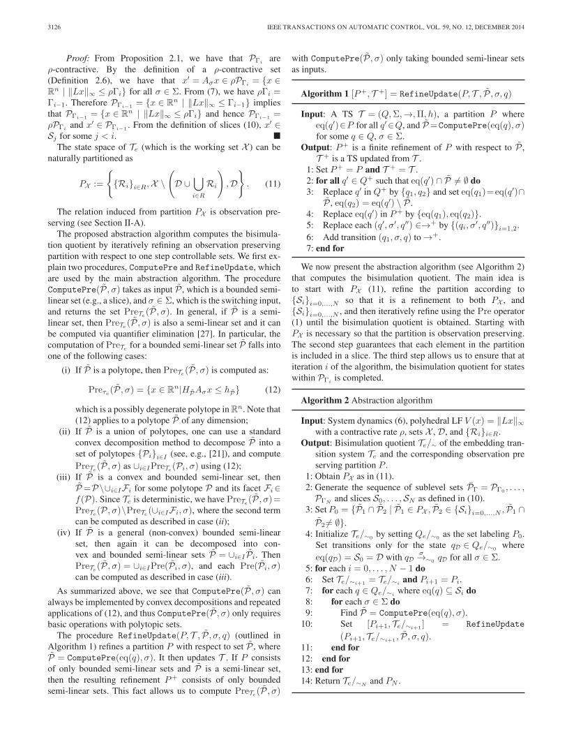
Fig. 7. The sets X , D, R1, R2, R3, and the sublevel sets PΓii=0,...,10of the Lyapunov function for Case Study 1.

the software package on an iMac with an Intel Core i5 processorat 2.8 GHz with 8 GB of memory. Algorithm 2 was completedin 2 hours for Example 3.1. Once the bisimulation quotientwas constructed, controller synthesis and verification were bothcompleted in 2 minutes.

A complete case study of a switched linear system in R2 waspresented as a running example throughout the paper. Here, twoadditional case studies are presented: a linear system in R3 anda piecewise linear system in R2.

A. Case Study 1

In this case study, we apply the proposed methods to a3-dimensional discrete-time linear system:

xk+1 =A1xk, where A1 =

⎡

⎣0.384 0.394 0.240

0 0.442 −0.442−0.100 0 0.780

⎤

⎦. (22)

The system is of the form (6) with Σ = 1. Note thatthe system is autonomous, i.e., there is only one dynamicsand therefore no control input. The system is asymptoticallystable and ∥Lx∥∞ is a Lyapunov function for the system withcontraction rate ρ = 0.91, where

L =

⎡

⎢⎢⎢⎢⎢⎢⎢⎢⎢⎢⎢⎢⎢⎢⎢⎢⎢⎣

−0.8835 0.1165 0.1165−0.8835 −0.1165 −0.11650.8835 −0.1165 −0.11650.8835 0.1165 0.1165

0 −1.0000 −0.11650 −1.0000 −0.11650 1.0000 0.11650 1.0000 0.11650 −0.1165 −1.00000 −0.1165 −1.00000 0.1165 1.00000 0.1165 1.0000

⎤

⎥⎥⎥⎥⎥⎥⎥⎥⎥⎥⎥⎥⎥⎥⎥⎥⎥⎦

.

The working set and the target set are X := x ∈R3 | ∥Lx∥∞ ≤ 10.0 and D = x ∈ R3 | ∥Lx∥∞ ≤ 3.8942,respectively. The sublevel sets PΓii=0,...,10 are computed asexplained in Section IV. These sublevel sets and the sets ofobservations, R = R1, R2, R3, are shown in Fig. 7.

Algorithm 2 was used to compute a finite bisimulation quo-tient of the corresponding embedding transition system. Thequotient TS had 14096 states and was computed in 35 minutes.

The following specification was considered: “A system tra-jectory either visits R1 and then R2, or R3 before visiting D.”The specification was formally stated as the following scLTLformula:

φ := (¬ΠD ∪ (R1 ∧ R3) ∧ ((¬R1 ∧ FR2) ∪ΠD) . (23)

The largest set of satisfying initial states of system (22)for formula Φ (23) was computed by following the methodsexplained in Section VI. The FSA had 5 states. Note thatboth the verification and synthesis problems result in the sameset for this case study, i.e., X S = X AS , since system (22) isautonomous. The computation of X S took 1.2 seconds. Thevolume of X S is 17.4% of the volume of X \ D. The set ofinitial states and sample trajectories are shown in Fig. 8.

B. Case Study 2

In this case study, we show how the proposed method to con-struct a bisimulation quotient can be applied to a piecewise lin-ear system. The system is adapted from [28], where stabilizingstatic feedback control laws for discrete-time piecewise affine(PWA) systems are synthesized. The synthesis framework in-volves computation of piecewise linear Lyapunov functions thatadmit piecewise polytopic sublevel sets. Here, we consider thestable closed-loop system which is described by (14) with:

A1 = A5 =

[0.0546 −0.77640.0212 −0.8521

]

A2 = A6 =

[−0.0700 −0.81500.0700 −0.7300

]

A3 = A7 =

[−0.9200 −0.02000.7580 −0.0200

]

A4 = A8 =

[−0.9200 0.02000.7580 −0.0200

]. (24)

We define the operating regions, Xσσ∈Σ, and the workingset, X = ∪σ∈ΣXσ , with respect to the conic partition of R2,Ωσσ∈Σ, used in [28] and the piecewise linear Lyapunovfunction of system:

V (x)=∥Lσx∥∞, if x∈Ωσ, Lσ∈Rl×n, l≥n, l∈Z+. (25)

The matrices, Lσσ∈Σ, of the Lyapunov function (25) areomitted due to space reasons, but can be found in [28]. We setΓX = 19.75 (PΓX = x ∈ Rn | V (x) ≤ ΓX as before) ΓD =10, and Xσ = X ∩ Ωσ for all σ ∈ Σ. The operating regions ofthe system and the sets Xσσ∈Σ and D are shown in Fig. 9.

The sublevel sets are not polytopic, however, the slices arestill bounded-semi linear sets and can be computed as explainedin Section IV. These slices and the regions of interests R areshown in Fig. 10. To find a bisimulation quotient for the system,we first refine partition PX (11) according to partition Ppwl =Xσσ∈Σ. This additional refinement step guarantees that each


Fig. 8. Case Study 1: (a) X S is shown in purple. (b) Four sample trajectories. The initial states are marked by circles. (c) The same trajectories as in (b) areshown under a different view angle (projected on x2 − x3 plane).

Fig. 9. Case Study 2: Xσσ∈Σ and D (shown in brown).

Fig. 10. Case Study 2: Slices Sii=0,...,11 and regions of observations R =

Rii=1,...,4. S4 is shown in purple.

P in the refined partition P pwlX is included in a set Xσ , and

therefore, only one mode can be active in P . As each set in P pwlX

is a bounded semi-linear set, Algorithm 2 is used to compute aquotient transition system Te/∼. By eliminating some of thetransitions according to Ppwl, i.e., q σ→∼ q′ only if eq(q) ⊆ Xσ,we obtain a bisimulation quotient T pwl

e /∼ for the piecewiselinear system. The computation took 11 minutes. Note that eachstate q of T pwl

e /∼ has a single outgoing transition, and thesystem is not controlled.

Fig. 11. Case Study 2: Satisfying initial states are shown in purple. Twosample trajectories are indicated by labeling.

We consider the specification: “A system trajectory nevervisits R2 and R4, and eventually visits R1 or R3,” whichtranslates to the following scLTL formula:

φ := (¬(R2 ∧ R4) ∪ΠD) ∧ F(R1 ∧ R3). (26)

The set of satisfying initial states of the system is foundby using the bisimulation quotient T pwl

e /∼ as explained inSection VI. As in the previous case study, both verification andsynthesis problems result in the same set, which is shown inFig. 11. The computation took 0.4 seconds.

VIII. CONCLUSION

In this paper, we presented a method to abstract the behaviorof a switched linear system within a positively invariant subset ofRn to a finite transition system via the construction of a bisim-ulation quotient. We employed polyhedral Lyapunov functionsto guide the partitioning of the state space and showed thatthe construction requires polytopic operations only. We showedhow this method can be used to synthesize switching sequencesand to verify the behavior of the system under arbitrary switch-ing from specifications given as scLTL formulae over polytopicsets in the state space of the system. We also describe how thisgeneral approach can be extended to verify piecewise linearsystems and systems with difference inclusion dynamics.


REFERENCES

[1] C. Belta et al., “Symbolic planning and control of robot motion [grandchallenges of robotics],” IEEE Robot. Autom. Mag., vol. 14, no. 1, pp. 61–70, Mar. 2007.

[2] S. G. Loizou and K. J. Kyriakopoulos, “Automatic synthesis of multiagentmotion tasks based on LTL specifications,” in Proc. IEEE Conf. DecisionControl, Paradise Islands, Bahamas, 2004, pp. 153–158.

[3] G. Batt et al., “Validation of qualitative models of genetic regulatorynetworks by model checking: Analysis of the nutritional stress response inescherichia coli,” Bioinformatics, vol. 21, no. S1, pp. i19–i28, Jun. 2005.

[4] R. Milner, Communication and Concurrency. Upper Saddle River, NJ,USA: Prentice-Hall, 1989.

[5] M. C. Browne, E. M. Clarke, and O. Grumberg, “Characterizing finitekripke structures in propositional temporal logic,” Theor. Comput. Sci.,vol. 59, no. 1/2, pp. 115–131, Jul. 1988.

[6] J. M. Davoren and A. Nerode, “Logics for hybrid systems,” Proc. IEEE,vol. 88, no. 7, pp. 985–1010, Jul. 2000.

[7] O. Kupferman and M. Y. Vardi, “Model checking of safety properties,”Formal Methods Syst. Des., vol. 19, no. 3, pp. 291–314, Nov. 2001.

[8] P. Tabuada and G. J. Pappas, “Linear time logic control of discrete-timelinear systems,” IEEE Trans. Autom. Control, vol. 51, no. 12, pp. 1862–1877, Dec. 2006.

[9] A. Chutinan and B. H. Krogh, “Verification of infinite-state dynamic sys-tems using approximate quotient transition systems,” IEEE Trans. Autom.Control, vol. 46, no. 9, pp. 1401–1410, Sep. 2001.

[10] R. Alur and D. L. Dill, “A theory of timed automata,” Theor. Comput. Sci.,vol. 126, no. 2, pp. 183–235, Apr. 1994.

[11] S. Sankaranarayanan and A. Tiwari, “Relational abstractions for contin-uous and hybrid systems,” in Computer Aided Verification, vol. 6806,G. Gopalakrishnan and S. Qadeer, Eds. Berlin, Germany: Springer-Verlag, 2011, ser. Lecture Notes in Computer Science, pp. 686–702.

[12] J. Piovesan, H. Tanner, and C. Abdallah, “Discrete asymptotic abstrac-tions of hybrid systems,” in Proc. IEEE Conf. Decision Control, 2006,pp. 917–922.

[13] B. Yordanov and C. Belta, “Formal analysis of discrete-time piecewiseaffine systems,” IEEE Trans. Autom. Control, vol. 55, no. 12, pp. 2834–2840, Dec. 2010.

[14] H. Lin and P. Antsaklis, “Stability and stabilizability of switched linearsystems: A survey of recent results,” IEEE Trans. Autom. Control, vol. 54,no. 2, pp. 308–322, Feb. 2009.

[15] A. Girard, G. Pola, and P. Tabuada, “Approximately bisimilar symbolicmodels for incrementally stable switched systems,” IEEE Trans. Autom.Control, vol. 55, no. 1, pp. 116–126, Jan. 2010.

[16] C. Sloth and R. Wisniewski, “Verification of continuous dynamical sys-tems by timed automata,” Formal Methods Syst. Des., vol. 39, no. 1,pp. 47–82, Aug. 2011.

[17] A. Girard and G. Pappas, “Approximation metrics for discrete and contin-uous systems,” IEEE Trans. Autom. Control, vol. 52, no. 5, pp. 782–798,May 2007.

[18] M. Zamani, G. Pola, M. Mazo, and P. Tabuada, “Symbolic models fornonlinear control systems without stability assumptions,” IEEE Trans.Autom. Control, vol. 57, no. 7, pp. 1804–1809, Jul. 2012.

[19] X. C. Ding, M. Lazar, and C. Belta, “Formal abstraction of linear systemsvia polyhedral Lyapunov functions,” in Proc. IFAC Conf. Anal. DesignHybrid Syst., Eindhoven, The Netherlands, Jun. 2012, pp. 88–93.

[20] E. A. Gol, X. C. Ding, M. Lazar, and C. Belta, “Finite bisimulations forswitched linear systems,” in Proc. IEEE Conf. Decision Control, 2012,pp. 7632–7637.

[21] B. Grünbaum, Convex Polytopes. New York, NY, USA: Springer-Verlag, 2003.

[22] Z. P. Jiang and Y. Wang, “A converse Lyapunov theorem for discrete-timesystems with disturbances,” Syst. Control Lett., vol. 45, no. 1, pp. 49–58,Jan. 2002.

[23] M. Lazar, “Model predictive control of hybrid systems: Stability androbustness,” Ph.D. dissertation, Eindhoven Univ. Technol., Eindhoven,The Netherlands, 2006.

[24] F. Blanchini, “Ultimate boundedness control for uncertain discrete-timesystems via set-induced Lyapunov functions,” IEEE Trans. Autom. Con-trol, vol. 39, no. 2, pp. 428–433, Feb. 1994.

[25] M. Lazar, “On infinity norms as Lyapunov functions: Alternative neces-sary and sufficient conditions,” in Proc. IEEE Conf. Decision Control,Atlanta, GA, USA, 2010, pp. 5936–5942.

[26] M. Kloetzer and C. Belta, “A fully automated framework for control oflinear systems from temporal logic specifications,” IEEE Trans. Autom.Control, vol. 53, no. 1, pp. 287–297, Feb. 2008.

[27] J. Bochnak, M. Coste, and M. F. Roy, Real Algebraic Geometry. Berlin,Germany: Springer-Verlag, 1998.

[28] M. Lazar and A. Jokic, “On infinity norms as Lyapunov functions forpiecewise affine systems,” in Hybrid Systems: Computation and Control.New York, NY, USA: ACM Press, 2010, pp. 131–140.

[29] E. M. Clarke, D. Peled, and O. Grumberg, Model Checking. Cambridge,MA, USA: MIT Press, 1999.

[30] Latvala, “Efficient model checking of safety properties,” in Proc. 10thInt. SPIN Workshop Model Checking Softw., Portland, OR, USA, 2003,pp. 74–88.

[31] M. Kloetzer and C. Belta, “Dealing with non-determinism in symboliccontrol,” in Hybrid Systems: Computation and Control, M. Egerstedt andB. Mishra, Eds. Berlin, Germany: Springer-Verlag, 2008, ser. LectureNotes in Computer Science, pp. 287–300.

[32] E. Asarin and O. Maler, “As soon as possible: Time optimal control fortimed automata,” in Hybrid Systems: Computation and Control. Berlin,Germany: Springer-Verlag, 1999, pp. 19–30.

Ebru Aydin Gol received the B.S. degree in com-puter engineering from Orta Dogu Teknik Üniver-sitesi, Ankara, Turkey, in 2008, the M.S. degreein computer science from Ecole PolytechniqueFèdèrale de Lausanne, Lausanne, Switzerland, in2010, and the Ph.D. degree in systems engineering atBoston University, Boston, MA, USA in 2014. Herresearch interests include verification and control ofdynamical systems, optimal control, and syntheticbiology.

Xuchu (Dennis) Ding received the B.S., M.S.,and Ph.D. degree in electrical and computer engi-neering from the Georgia Institute of Technology,Atlanta, in 2004, 2007 and 2009, respectively. Dur-ing 2010 to 2011 he was a postdoctoral researchfellow at Boston University. In 2011 he joined UnitedTechnologies Research Center as a Senior ResearchScientist. His research interests include hierarchi-cal mission planning with formal guarantees underdynamic and rich environments, optimal control ofhybrid systems, and coordination of multi-agent net-

worked systems.

Mircea Lazar (born in Iasi, Romania, 1978) re-ceived the M.Sc. and Ph.D. degrees in controlengineering from the Technical University “Gh.Asachi” of Iasi, Romania (2002) and the EindhovenUniversity of Technology, The Netherlands (2006),respectively. For the PhD thesis he received the Euro-pean Embedded Control Institute (EECI) PhD award.Since 2006 he has been an Assistant Professor in theControl Systems group of the Electrical EngineeringFaculty at the Eindhoven University of Technology.His research interests lie in stability theory, scalable

Lyapunov methods and formal methods, and model predictive control.

Calin Belta is an Associate Professor in the De-partment of Mechanical Engineering, Department ofElectrical and Computer Engineering, and the Divi-sion of Systems Engineering at Boston University.His research focuses on dynamics and control the-ory, with particular emphasis on hybrid and cyber-physical systems, formal synthesis and verification,and applications in robotics and systems biology.Calin Belta is a Senior Member of the IEEE and anAssociate Editor for the SIAM Journal on Controland Optimization (SICON). He received the Air

Force Office of Scientific Research Young Investigator Award and the NationalScience Foundation CAREER Award.

3122 ieee transactions on automatic...

Documents