t:T-

OF CONTROL SYSTEMS

6.I INPUT SICNALS

Conhol systems are basically dynamic systems So' studying lhetu, behaviour with tine

;";;-i;t. Indeed, the study of variaiion of output of a control system is important

;r;;;y;tp*tiues it cluding its stabiLity ToYuy*l ttle actual inPut to the. syste:l

;-;;t"u"';r.";*" and, therefoie, some siandard test inPrrt signals are used in the

;d;: #" ait.t*"a "".i't

srgnals in Chapter 2 (Section 2 7) and their LaPlace traff-

fo.u'G. Here, we summarise them in Table 6 t'

31'n . -ur- V.ar/ *1

A'*/Ja. c".,t""I-rl , I t| tu rd' Cr!1t

TIME DOMAIN PERFORMANCE

Table 6.1 Standard test signals

R(s)/(t)Signdl

Unit imPulse

Unit step

Unit ramP

Unit patabolic

/(f) = 1

tzP\ t )= i

v{6(f)} = 1

YIU{t)l

{lt(t)l

r,lp(I)l

l r^ l for o <t<et( f )=l€-o€

f0 fo r t>e

[0 fo r fS0a(t) =

{t for r >o

15

1

1s3

Itinte$al

may be noted from the Laplace transforms

of the preceding one.

136

that each successive signal is the

Time Domain Perlormance ol Contrcl Svstems 137

6.2 RESPONSES

Once an input is given to a system, it will produce an output or response. The responsecan be (i) transient or (ii) steady-staie.

The hansient response is that palt of the response which approaches to zero astime tends to infinity. The part of the response that remains after the transients die outis called the steady-state resporue. The parameter, which is important in the steadystate, is the steady-state ellor, ers. It is defined as

ess = lim e(f)

= lim [r(0 - c(t)

where e(t), being the difference between reference input r(l) and output c(f), is the error.

6.3 TIME RESPONSE ANALYSIS: FIRST ORDER SYSTEM

If the dlnamic relation between the reference input /(r) and output.(t) of a system isof the form of

then it car be wdtten as

a1ff+ a6c(t) = bor(t)

rp-+4t1=xr1t1a t

where r = alao = firf.e constant ard K = bo/qo = gain of the system. Taking the Laplacetrarsform of Eq. (6.3) and assuming all initial conditions = Q we have

(6.1)

(6.2)

(63)

(6.4)

(6.s)

(s?+ 1)C(s) = KR(s)

Equation (5.4) yields the transfer firnction as

^. C(s) (( J ( S ) = : = -" R(s) sr+1

The order of the transfer function is 1. So, such systems are called fust order systems.The block diagram and the signal flow graph of a first order system are given inFigure 6.1.

(4.) (b)

Figure 6.1 Firs't oider system: (a) block diagram and (b) signal flow graph.

Now, we check the resporue of the system for diflerent standard inputs.

1sf

138 lntroduction to Linear and Digital Contrcl systems

6.3.1 Unit lmpulse Input

Since for the unit impulse inPut R(s) = 1, we have

1C(s) = ---:--;

s t + l

=-.------'

" * ;

On tai..ing the inverse LaPlace transform, we 8et

cG\ =: e-;

So,

The tine-response curve is

0 t

Figure 6.2 Timsresponse curv€ lor unit impulse input.

6.3.2 Unit Step Input

In the case of the unit step inPut, R(s) = 175. Therefore,

^ . . 1 1L(s)=- . -

S S C + I

11=;---T' t * ;

which on the inverse Laplace transform yields

t

c(t) =7 - e t

1c(t) -+ :

c(t) r 0

6.2.

(6.8)

(6.e)

Time Domain Pertomance of Controlsystems 139

It may be obsewed from Eq. (6.9) that

lnifial sloPe of the cu*e =dc(tll

1 -1 I=-e t I

1r

We see from Eq. (6.10) that if the value of r is high, ihe initial slope is low and vice

versa. Thus, the lower is t the faster is the response' Also, the lower is r, the Ngher

is the stability. This is aPparent from a plot of its poles (see Figure 6 3 where a Plot is

shown for hvo values o]-t with q > tr' Here the transfer function may be obtained

from Eq. (6.8) as

-. . C(s) 1G(s) =

L(,) =;

+ 1

Poles are obtained by solving the charactedstic equation sr+ 1 = 0, yielding s = -l/r'

(6.10)

(5.11)

Flgure 6,3 Plot ol poles of a closedloop lirst order system

The steady-state error is given as

es, = lim k(t) - c(f)l = 1 - 1= 0

This result js obiained from the time-resporue of the s)"stem. without finding out the

time.response, i.e., without doing inverse Laplace transform, we can find out the steady-

state error by applying the finai value theorem. we will discuss the method later (see

Section 6.5).An interesting result may be obtained from Table 6'2 where the values of the

output are givm igainst t/l. lt may be seen that the step response of the first order

sysiem attaiiu 99.3i" of the final value for t = 5't ' The time-response curve is shown

in Figure 6.4.

140 lntoduction to Linear and Digital Control Systems

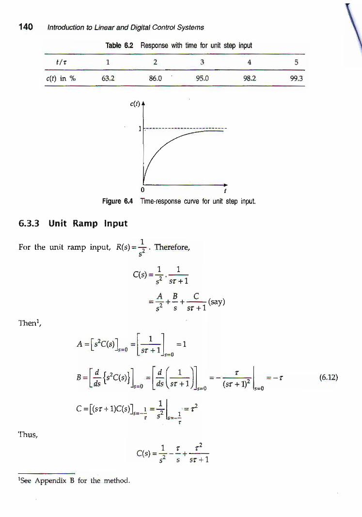
Table 6.2 Response with time for unit step input

t / r

c(t) in % 63.2 86.0 95.0 982 99.3

c(t)

I

6.3.3

For the

I nen"

0 tFigule 6.4 Time'response cuffe for unit step input.

unit Ramp Input

1unit ramp input, R(s)=; Therefore,

'I 1

s- sr+r

AB C=;+-+------;.(saf)s ' s 5 t+ I

t1 l= l - t - _L

lsr+11 ^

t,,.,,,]]"_, = [,i (rh)],=, = _ d7l"=,= _ "1

a =is'?ctsll ^

=l+L A S

=[G"

(6.12',)

+ - t l L t s l l I =i l

Thus,

lSee Appendix B for the method.

' l r r z

C(s)=+-'+ :s ' s s t+r

Tine Domain Perlormance of Contol Systems

1t t=- t - -+ - - - -Ts - s s+ j

twhich on the inverse Laplace transforrn yields

-:c ( t ) = t - a 1 7 2 t

r -1)=t-t lL-e " I

\ , /

The timeresponse curve is given in Figure 6.5. The steady-state eEor is given

e* = tim [r(r) - c(f)]- - t t_

= t - (t - z) From Eq. (6.14)1

Table 6.3 Mrnual relationship between inpul and response

141

(6.13)

(6.14)

(6.1s)

Flgure 6,5 Time"r€sponse curve for the unit ramp input.

We find ftom Table 6.3 that the interrelation between different inputs also holds goodfor the corresponding responses.

Input, r(t) Response, c(t)Reldtionship Relationship

Rampr(t) = t

u(t) = 1

Impulse

d(4

dr(t\dt 7- e' t / t *orl,,*

1- !t*,^,,1,=" *n l"-,

ila Eitoduction to Linear and Digital Control Systems

6,4 TIME-RESPONSE ANALYSIS: SECOND ORDER SYSTEM

Ii tl€ d]'namic input-outPut relationshiP of a system is rePresented by a differential

equation of the form oI

o^ d"\') * 0.4!ll 1 ao6(1) = !or(1)

'd {a t(6.16)

(6.77)

(6.18)

i i isca l ledasecondordersystembecausewewi l lpresent lyseethat thet rar rs fer func-tion of the system has an order of 2'

Eouation (6.16) can be written as

1 dzclt) *2€ dclt) +c(f)=Kr(f)c'* dt2 a" dt

'1_ - az

, 2q =a, , ^d K =b

oi ao 0n as 40

"*iil$|,iJl'ii'f*x\i#il#?"{#l#il";,'W'ff ,7,"^#u^JJ1*'#ii'*i'ro["'^iii-J-tt+"- ii."., utt

-ittltl"t conditions = 0)' we get

l++:! :+1lc(s)=KRG)\ ar; an )

where

On rearranging Eq. (61E), we get the transfer function for the secsrd order system as

car=ffi=;l-fi4' ,, -'

, , , -z=7.rlz.s;A

This can also be written in the form

cG)- KR(s) s(s? +1) + K

. {

= -.-.-L..-;

rS r \s_ +-+-

K"_ =ai7

where

(6.1e)

Time Domain Peiomance ot Control Systems 143

and (6.20)

2at

The results given in Eq. (6.20) are inportant because they indicate how the undampednatural frequency and damping ratio behave with the gain, With the increase in gain,the natural frequency increases which, in turn, reduces the damping ratio.

The block diagram and signal flow graph representations of a second order systemare given in Figure 6.6.

(a) (b)

Figure 6.6 Second order syslem: (a) block diagram and {b) signal flow graplr.

From Eq. (6.20) we see that the characteristic equation for the system is

sz +2fatns + afi =o

Therefore, its roots are given by

(6.21)

sr, s, = -(o, ! a" ,t€'z1 (6.22)

Depending on the value of (, three distinct cases present themselves from Eq. (6.22)as shown in Table 6.4.

Table 6.4 Three distinct cases of second order svsiems

txYT

124@- =:

t

€ =

Danping ntioxalue

Roots of charactetisticeq .Ltion

S!stefllspecifcatian

123

E> 1

E<I

r t r 12 dLu

q = s2 and both are real.s1 and s2 are complex, one beingthe coniugate of the other.

Overdamped

Critically damped

Underdamped

We will consider only the r.nit step input for the second order system.

14 lntrodlrdion to LineAr. aN Digitat Contrct S}fl{ems

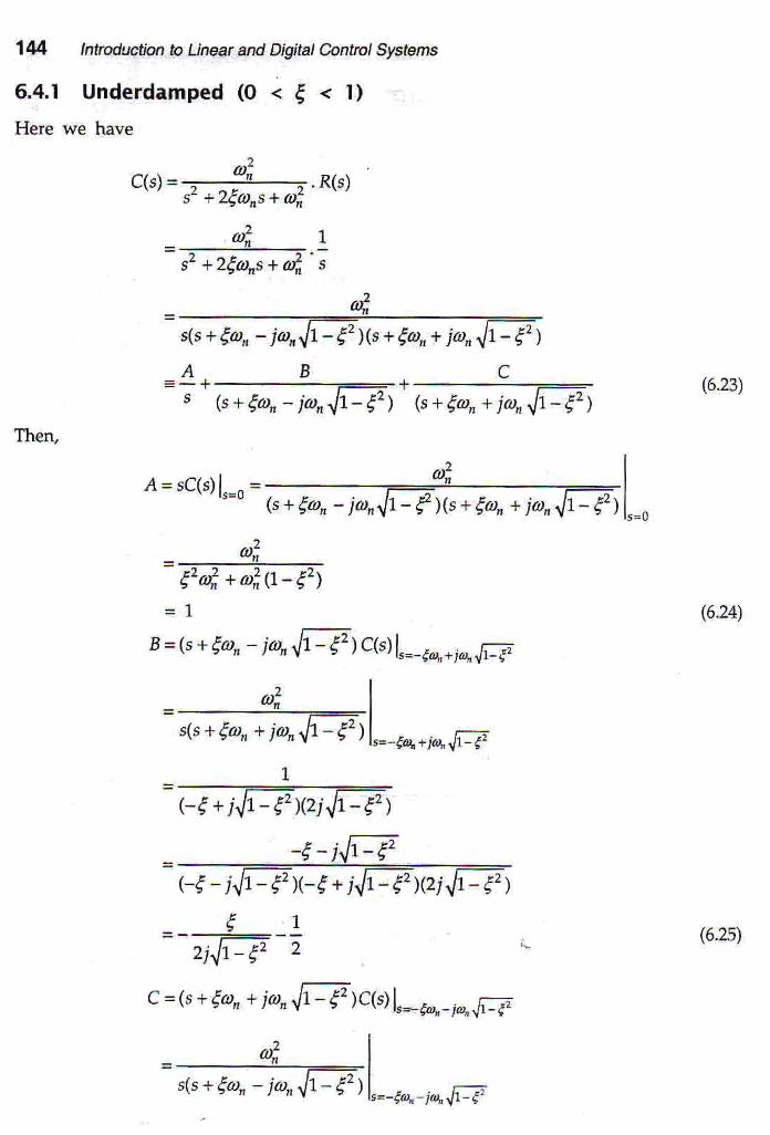
6.4.1 Underdamped (O < 6 < t)Here we have

Thery

c(')=T;#;a R(,)

-4, B cs 1s+(a,- jr,, l t-Crl k+(a4 + 1a,,t l-y'1

e=sc(s)1.=. = =,1 |' - (s + €a, - ja,1l1 _ ()(s + fa, + iat,,tt_ 6r)1,=o

="t€'d * r,*Q- €')

- F2 v r ;

(6.%)

(6.24)

t1 * z€r,t * ,4, 'i

s(s + (a, - jro,,t1. - (2 11s + (a, + ia^ .fi - 62 1

et-i l l-€'z)F€+

(6.:2s)

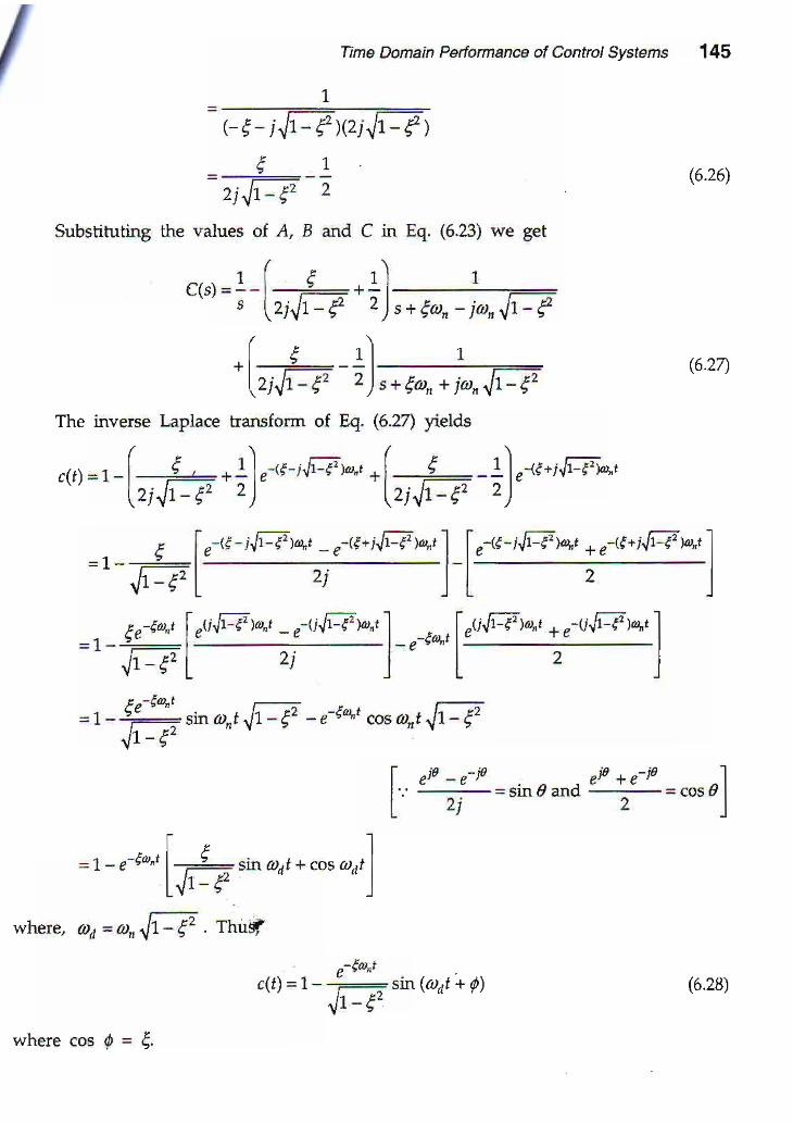
Time Domain Petformance of Contrcl Systems 145

^ : h E 2 )z J ! \ _e

Substituting dre values of 4, B ard C in Eq.

' t ( , ' ' )

!151=: - l - - - !+ : l

" l2i,l1-e 2)

(6.23) we get

1

s+(a,- jo4^l l j

1

(6.26)

(6.27)( E 1l-l;@-21

s + (a, + ia, rll-1,The inverse Laplace trarsfom of Eq. (6.27) yields

( - . \ ( " - \

( r )=I- |_9 + ! l r - tq- i ' l t -E ' t ' . ' * I -L-1|"<1uiJt-€ ' t ' " rlzj^lt-€' 2) lzj, lt-€, 2)

. € l r-,e -i,F:F,^' - r<e-i[4-w,,f l r-,t-i,!14w, *r-c.i,FZw,,l='-El ,i j-L ' l=t _ ia2r=l,ti[4,.t _,-,i'FT,,' )_,-r*,1,,i[7,^' *_"-u,FT,^'1

^lt-E,L 2j j L 2 )E--1a"1=t-ffi" r,tSI -r+^,'

"orr"t,[-y'I eie - p-ie - eF +e-F l

L 4 =t 'oaro -=cosal

= | - e-c@rl L,^ r,, - "or,,,lj lt-e "l

wherc, os4 =r,,{11 . m"sf

"(t)=t-ffi"a(aat+O)wherecosf={ .

(6.28)

to Linear and Digital Control S'rsterns

"<t) 2

I

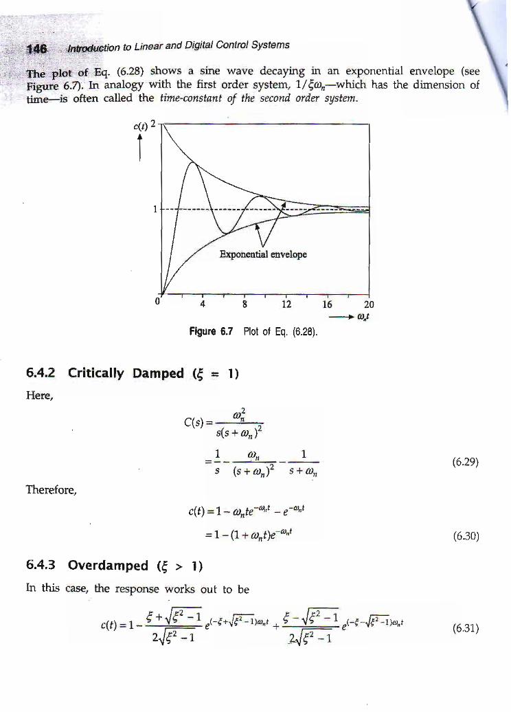
Figue 6.? ptot of Eq. (0.2a). a

6.4.2 Critically Damped (6 = r )Here,

ffi&. (6.28) shows a -sine wave decaying.,in an exponential envelope (seeif-, h arylogy udth the fi$t order systerL 1/6a+_which has the dimension ofi often called tJne thrle-mnstsnt of the'seconi orier"system-

- -* -

aiL(sl = ----ij-

s(s + aL)''L a"s (s + ro)2 s+an

Therefore,

c(t) =7 - o#e-aa,t - e-qt

=7-(7+a,t)e-,t

(6.2e)

(5.30)

6,4.3 Overdamped (6 > I )In th.is case, the response work out to be

,1,1 =, - Lfr ,t-€-'!Fiw,r * L-JVi- ",-, -E u,,,,,2,,1€, -1 zJP= "

Exponcntial covElopc

(6.30

lime Domain Peiormance ot Control Systems 147

The response curves for cdtically damPed and over-damPed systems are given m

Fgure 6.8.

o 2 4 6 ,__________ J"

Figule 6,8 Response curves for critically damped and overdamped sysiems.

It is apparent from the curves that the more is the value of t the more is the rise time

and, tirerefore, ihe settling time. Also, it can be seen from the cuwe that a criiica1y-

darnped second order system attains the step inPut value at the time constant value of

nearly 8 while this value was nearly 5 for the first order system'

6.4.4 Performance Parameters for Transient Response

The relevant Parametels are defined in Table 6.5.

Table 65 Perlomance Parameters

c(t)

1''

,/ - Cdticany drnPed (E = 1.0)

,,' ----- overdrnp€dc= l.t

Pararnetet Defnition

Delay time, t4

Rise time, J'

Peak time, tp

Maximum overshoot, Mp

Settling time, t'

The time required fo! the steP response of the system to reach50% of the final value.

The time required for the steP resPonse to reach the final outPutfor the ftst time in underdamPed systems or Srow from 10% to90% of the value in overdamped systems

The time required by the steP resPonse of the system to reach thefirst peak which is the maximum value of the output.

The maximum amount by which the outPut deviates from theinput. It is generally expressed as Per cent of the inPut.

The time the s,'stem takes to settle within a giv€n Per cent of the

final value.

These parameters are graphically Presented in FiSure 6'9 for the steP resPonse of a

second order sYstem.

148 lntod^ction to Lineat and Digital Contrcl Systems

c(t) t et '"I

t.2

0.8

Figure 6,9 Graphical pr€sentation of performance param;o|

Nov/, let us discuss these parameters one by one.Delay time

Ior (> '1

x=7+0.7EEquation (6.33) yields ihe approximate expression for d as

. 1+ o.zeorn

t

0.4

0.0

According to the definitiory ,(t)1,=,, =;. So, from Eqs. (6.28), (6.30) and (6.31) we get

( t+x)e- '= |

5 r-{!-:! "r-e',"t}-r " *1-,1(

-1 "r-:-,ng-rr

=12'l( -t z,lg, -t -

2wnere : = arola. Solutions to Eo. (6.32) carr be obtained for diJferent values of f arrdpol,lni.'[,,ffii graph of { u'

". A ti.,"", "pp.;,";;;"-i; iJ, g,"pll ts siven uy the

Rise timeWe consider the underdamped system for simplicity. If t, = 1i,o" requued to attain thesteady_-state value, we noti that ihe sine facto^r .f iiq. 1O.Zey'rf,orid harr" a ,ero ualoeto make c(r) = 1. Thus, from Eq. (6.28), we get

(6.32)

(6.33)

(6.34)

i-1,\Y,

- - - - - - - - - - - - - - - - - t , - - - - - - - - - - - - - - _ _ _ _ - _ ;

str.(adt + lt_t, =0=sinNz (6.3s)

Time Domain Pertotmance of hntrol Systems

first time, i.e., for N = 1, we have from Eq. (6.34)

|'..._-. , ' h r 'tDnt t l t -5 - +cos 'E=E

. n - cos-l E (6.36)

ad cos (0d, + il - E@^ sin (odtp + 0) = 0

|---Jt - f'z cos 11ar".it - oz \tp + 01- € s:u;.l(a, 11'-,,')te+Ql=0

i--------=

sin / cos [(a,, ,lt- ro'1to +/]-cosCsin(ar, 17-a')tp+0)=0

snl@,,[-FYr+/-/ ]=o=sinNz 6s7)

For the first peak, N = 1' Therefore,

L=-.L' , ,Jt- i '(5.38)

(5.3e)

a little algebraic

(6.40)

149

Peak time

ff t" = time required to reach the first pea! we can find an expression for it from

rq.is.za1 using -tfte

condition that c(f) will be maximum here' Thus,

-to"t" ,n, o-1r,t"dc\t) | =-lJt" cos (r,t"t, + 61n2!! sin (rd,rt, +d)=0dt 1,, Jt-g' ,!r-f

Maximum overshootSince it is the overshoot value at the Peak tirne,

Mr=c(t )1,_ro_.1

--1o"i l

fusrnfta,./t -(ltr+P1

Substituting lo value from Eq. (6'38) h Eq (6'39), we get after

rnanipulation

-i-Mo = s r'- '

Maximun per cent overchoot can be obtained by rnultiplyin-g the righFhand side ofgq. fO.+Ol Uy 100. Ii may be observed that Mo is a function of { only' Its behaviour with

f is shown in Figue 6.10'

^ t ; ,2

150 tntroduction to Linear and Digital Contrcl Systems

'/oMe IOO

tl,oI

60

Settling timeIf ts = time for settling within 2% of the final value, then

5@"

This approximate relation can be arrived at from the following considerations. Supposewe want that the output settles u/ithin a tolerance band of tA. That means, the arnpli-tude of the oscillating sine factor shoutd equal A Therefore,

t -=A

Vl - 9-Taking the logarithm of both sides of Eq. (6.42) and on rearranging, we ger

0

Flgure 6.10 6 vs Mp ptot.

-€atS"=rr6.,trj1

=]nA-: -2

. t InAt - = + - -' 2an €o"

Since f < 1, the second term on the right-hand side of Eq. (6.43) doninates and so wemay write it as

t =-++ $.44)Eo"Substituting A = 0.02 in Eq. (6.M), we get the approximate reiation of Eat. 6.aU.

(6.4-L)

(6.42)

(6.43)

Tme Domain Perlormance ol conttol systems 151

SteadY'state error

From the definition of error--|'i"l

e( = r\r\ - c0 = kV

s\^(ali + Q)

eo=e(r)L--=0

j'1#",':$tr1';{.'##j{liill':'#iffil'For a unity feedback system having

LcG)=a;l6i

find (a) o+' (b) € (c) ara (d) ro and (e) Mo'

Solution: Since it is a unity f""aUutt 'yu"'n' its overall transfer function is grven

by rG)=#%

With this

lems and then

to calculation

EXAi/IPLE 6.t

25s(s+10)+25

25s2 +10s+25

a]"=---------

sz + Z(tons + a4

the given transfer function with

(criticallY damPed)

(6.4s)

(6'46)

out a few Prob-having recourse

that of the stan-

ComParing the denomirators of

da-rd second order system' we ger

(a)

(b)

(c)

ai =zc

an = 5 tad/s

z(a, = L0

,=5 ' - l

l - c z _ i( D d = . / J n l L - 9 - w

cG)=:- +:s(r+s l ,

where T and K are Positive constants. By what factor should the gain K be

that(a) the peak overshoot of the system to unit steP input is reduced

25o/", auld(b) the damping ratio increases from 0.1 to 0 5?

Solution: The overall hansfer function of the system is given by

152 lntroduction to Linear and Digital Control Systems

b=--#'+*(noveak)

Mp = 0, since it has no Peak.

The open-loop transfer function of a unity feedback system is glven by

reduced sudr

from 75olo to

rr"r = G(s)- ' - '

1+G(s)

Ks(1+sT)+K

K/T=" s n- 'T 'T

(r)- s2 + 2(ans + c']

(d)

(e)

EXAIiIPLE 6.2

By comparison we get

(a) From Eq. (6.40) we

On taking the logarithms of

(ii)

(iir)

-G

1o;"=.tK/T *rd €=ft.

--+-^^ .tr- ti

\Mp)1= Lwe ' " = / J

,t'--/rr \ - inn- ,! t- i i -oE,\tvlp 12 - Lw.

both sides, vre get

-ffi=nffi=rn3-rn4

ln4- ln3 ^^^ . ,= - = U'u, loOI(i")

(-^

Time Domain Peiormance ot Contrcl Systems

l n 4 - l n 1= ::j_:___:- = 0.4413

1S|

(v,-ffi

(vi)or

("ii)

(viii)

reduced to lower the Peak

(ix)

/(t) = sin t

RG)=-5fs -+1

Equathg the numeratols of both sides, we get from comPadng the coe{ficientss6, *, sa, s3, s2, s and the constant

Substituting E =# ^^ €r=#, we get from Eqs. (iv) and (v)

r ^ ̂ ^..: = U , V Y I o

J4KJ -1,

K1T = 30.045"t ^ , , . .

-=u. '+4t lJ,l4K2T -1,

or K2T = 7.534

Thus from Eqs. (vi) and (vii), we get

K. 30.045 -^ _^-- = - = I y . 5 d oK2 "1.5U

Equation (viii) suggests that K should be nearly 20 timbsovershoot ftom 75'/" to 25"/".

(b) Here,

€,=w_€z \ KtT

(, e] (o.ef ̂ -.j =: = ---------- = JoK2 €i (0.7)'

The import of Eq. (ix) is that K has to decrease to 1/36 ot its Present value to increase

the damping ratio lrom 0.1 to 0.6

EXAMPLE 6.3 Find ihe time response of the following system for inPut r(t) = sin t'

"(s) = ---1-' ' (s+ l ) (s '+1)

Solution:

154 lntoduction to Linear and Digital Antol Systems

1111 ' ]A=l,B=-: 'c=:. D= : and r=;

42244

Thus,I 1 1 s - l 1 ' - l

L(J) -a. s+ I

- t . ( r r_ i ) t - 4 ?;

1 1 1 s I 1 1 s .1 1T- . - : - - - - - - - - - i - _ - : . - ; - - - - ' -- I ' s+ t -Z

[ t+ f12 '2 G2 +1)2 4 s2+1 4 s?+1

On performing inverse LaPlace transfoLm,

. . 1 ' 1C 1 1 1c(t)=:ct- rVUsnn*;t

s inf - icmf -Nsint

=1r-t -1r* r - l tcost +1 tsin t - lcos t +]sint4 ' 2 - 2 2 4 4

. t 1 ( . n \ 1 ( . t r \=ae-t - -#sinl r +T l++rsinl t - ; I4 2 ,12 \ 4 .J 42 \ 4 /

EXAITPLE 6.4 A step inPut is applied to a unity feedback sl"stem having the following

openloop transfer function:

u(s)=s(s+3)

Find (a) the closed-loop Fansfer functiort (b) at, (c) { and (d) (d,i.

Solution:

(a) Closed-loop transfer tunction =i%==+* = ̂ z tS

1+C(s) s (s+3)+15 < '+35-15

(b) Comparing the denominator of the closed-loop transfer ftnction with that of astandard second order transfer fun€tiory we get

1ti =1'5

or a, -- JE =3 873 rad/s

(c) From the same compadson, we also get

z(tt' = 3

t= 3 =-L=o.sez' 2a,, 2.1"15

(d) ,n=r, , [ - { = 3.57rrad/ s

fII

a{At PLE 6.5 A second order confrol

;biected to a steP inPut Determine (a)

(b)

(c,

(d)

Time Domain Performance ol Contolsystems 155

system, having 6 = 04 and au = 5 rad/s, isilosedJoop transfer function, (b) t., (c) tp, (d) L

and (e) Mr'

Solulion:(a) The siandard closed-loop transfer function for a second order control system i5

given bY

c(s) alRC\=j.'zA"*4

Substituting the values of g and a)", we gei

C(s) 25R(s) s' + 4s + 25

t t - cos- ' t n-cos- l 0 .4 ^ ,. = :=- - . ' *33s' , ,$-4 5Ji-016

, =---L=---L-=166,' ' t ,Jt-* sJ1-0'16

44t"= fu,= (u4)(r= '"

(e)

EXAMPLE 6,6function:

%M, = 1se "' (- ft)=', ",.' [- ffi] = *,

14c+t s+; A B

t r > ; = - - - _ - - i . ; = : ' = - , . - I' ' (2s +7\ ' f 1 \ ' f 1 \l '-;J t'*tJ '-t

A unity feedback control system has the following oPen-looP transfer

^ . 4s+ lU tS )= -

4s'

Find expressions for its time response when it is subiected to (a) unit imPulse inPui and

(b) unit steP rnPut.

Solulion: The closed-loop transfer function of the system is given by

- C(s) 4s+1 4s+7- ' - '

R(s) 4sr + 45 + I (2s ' i ) '

(a) For a unit impulse inPut, R(s) = 1.

Thus,

co=- /+l'++ul'*;) '*,The inverse Laplace trarsform of the above equation yields

,6="4 _!pi=1,_i]r:

(b) For a unit step input, R(s)=]. f:herefore

7

cG\= ( +=+*, j;g*{ t,"yr

'l'n tJ ['.;J '*,

,*1 I.,{=sc(s)1,_o=a+l =l['*rJ l"=,

1'56 tntoduclion to Linear and Digital Contol Systems

Thert

)'.u,t=+ =(,.i),= ,.r)'.,0]"__, =*(,.

2

1+-2

tl'- -

\ -

)

ds

1 l/ i \ 2 | s+ : l

^ I r l - . . 1 a l 1 ,D= ls+; lc (s ) l = - - -a l\ zJ I I s I 2

- l s = - :2

1 \ l/ L | 1

z

.=f,{(,'};'.r,,}L_,=*{+}l =i: +---, t Jl.=_r L

12

Thus,

lE inverse LaPlace transform yields

Figure 6'11 Block diagram of the control

Solution: The block diagram can be reduced

Time Domain Peiormance ol control systems 157

system (Example 6.7).

as shown in Figure 6.11(a).

. | | | r r Ic t1= j +!k1 -e-z =t - l t - : ls z. 2 \ z /

E(AtilPLE 6.7 Determine the trarsfer function of the control system given in flguJe Ort]

ffi"i"-ri* ur.""pression for its output if the input is a step having a magnitude of 2

units,

Flgure 6.11(a)

The reduced block diagram yields the closed-loop ftansfer function of the ryrstem as

C(s) 4T/<\ =: l :1= :' ' " '

RG) s(s+4)+4+4(s+2)

4=7;8s+12

4

(s+2)(s+6)

r(s 'f 4) + 4

158 ln oduction to Linear and Digitat Control Systems

JGiven, R(s) =: . Therefore,

s

cG)=so;is+6)

=A* B=*-!_1r"y15 S+ l 5+6

Then,

A=sC(s)l =81=?' ' 's=u (s + 2Xs + 6) l._o 3

B=(s+2)c(s)1"__, =Girl"= , =_,

C=(s+6)C(s) l =81=:' ' ' s=-o s(s+2) l 3

Thus,

cG)=:.1_++1.+J s s+z J s+6

Its inverse Laplace traasform yields

c1t\ =2, - e-^ a !2alC J

EXAMPLE 6.8 Measurement conducted on a servomechanism shows the error responseto be

e(t) = 1.66e-8t sin (6f + 32")where the input is a sudden unit displacement, Determine the natural frequency, damp_ing ratio and damped angular frequerLcy of the system.

Solution: Given, r(f) = 1. 11"r"1ot"

e( f )=r (s ) -c ( t )=1-c0)

Since the error is sinusoidal, it is a second order underdamped system where for a stepiltput

"-go"tc(t)=1--:......".-s (adt + cos-1 €)

Therefore,

ao=#"*t'rr+cos-1 4)

Time Donain Pertormance ol Contrd Systems

= L.56eit sin (51 + 37.) (given)

By comparisorL

cos-l 6 = 37"

€ = cos 37" = 0.7986

aa = 6 rad/s

A_ = ---:= = Y.YOY raa/s"ha

EXAfITPLE 6.9 In the block diagram shown in Figrue 6.12, G(s) = A/g and H(s) = 25 a 2'For A = 1O determine the values ol m and n for a step inPut with a time{onstant 01 swhich gives a peak overshoot of 30%

159

Solution: The

Figure 6.12 Block diagram (Example 6.9).

overall transfer furction of the system is given by

rG)=:9= G(s)''

R(s) 1+G(s)H(s)

A= s '+A- t+A"

ntZ= _________::t!--

sz+\ las,s+tf i

Comparing the denominators, we get

2ean=An=10m

afi = 4n =19,

From Eq. (i) we find

(i)

. 10m 10m' 20n 2.t10n

Time constant . - ==: -=:=0.1s (g iven)60,, )Um 5f i

Now,

(ii)

t60 lntoduction to Linear and Digital Contol Systems

\m=2

Substituting tllis value in Eq. (ii), we get

, 10 x2 l05=iFo"=ffiAg"lru

(iii)

( -, '\

reak overshoot, "/olv\ = r00 exp l_ ff iJ

= ro <sivenl

-$=*e.31=-1-2sav t - 9

1tz€2 = (7.204)2 (1 _ €2)

e=IE=ouu,nThus, substituting the value of f in Eq. (iii), we get

/rn,l- = 0.3579ln

,=ffi=ze.ozEXAITPLE 6.10 A sysrem and irsDetermine tre values ot ,r,r, a u.J?o*e

curve ;ue given in Figue 6'13(a) and (b)'

(ar G)Flgure 6.13 Example 6,10: (a) th6 system and (b) the responso.

II

I Tine Domain Petformance af Control Systems 161

Solution: The differmtial equation for the system can be wdtten as

Mdzxl t , ) r Bdx( t ) +Kr( f )=y(r )df dt

Its l-aplace transform, for all initial conditions = 0' is

(szM + sB + r0 XG) = Y(s)

Therefore, the transfer function of the system is

r(,)=#=7r*+K1/M=j;T;E,

This yields the characteristic equahon

.r*9r*I=o=r2 +z(at,s + t f i.M-M

By comParison we gef

Now, peak overshoot

zio"=fr

BBF = --,-:-- =:' 2a"M z.JY'M

(i)

(ii)

*, = .*l- #,)=

o $! 1r'o-'""ponse cuwe)

ft=-.o'oeu=zzzos(in)

From Figure 613(a) and Eq (i)

xG) =s(Msz+Bs+K)

8.9

8.9 8'9r(-) =0.03 =1im sx(s) = Igt

Mst;s + K =?-

So,

Conlrol Systems

x=ffi=2e6.67p7*

1 = --ft = z{ from resPonse)o,

"11- 5 '

(v)

(vi)

B2.IKM

= 2(0.se7 \ J Qe 6.67 \n s$)

Figure 6,14 Closed.loop system (Example 6.11).

The overall trarufer function of the svsrem rs

_. . C(s) K. l t 5 t = - = -'

R(s) s(s+a)+K

= 1.958 radls

Combining the results of Eqs. (iv) and (v), we get

',=ffi=''*'v 1041,,

rvt =---. =.-- = / /,365 Ke,)z /1 Oq9\z

And Eq. (ii) together with Eq. (vi) yields

€ =

B =2€JKNl

= 180.91 N-s/m

EXAIIPLE 6.|1 In the closed-loop system shown in Figurc 6.14, determine the value ofK and a such that the per cent peak overshoot due to the unit step input does notexceed 10%. Settling time should be equal to 1s.

Solution:

/

Time Donain Peiormance of Control Systems

K

s2+ns+K

Comparing the chamcteristic equation, s2 + 4s + ( = 0, with that of a standard second

order system, we get

a)" = Vrr

.aa' 2ah zJK

fs =-= ls(8rven)

€ro, = +g .

= - lusrng !,q. (r,l

a=8

16il

Now,

(i)

(ii)

(in)

Ttre peak overshoot condition gives us

( - , \exP!- ; ! 1= g '1

| .'/1 -6' j

=2.303

Substituting the value of { from Eq. (i) in Eq. (iii), we get

nE-7-

Putting the value

^ 1 ,-+=2.303l" n'

\ l ' - 4K

t--------"'= -'---

t!4K - a'

of a from Eq. (ii) h tl:ris equatiorL we get

n(8\- = Z . J U J

,l4K - 64

64tt2

2.303'

. . 11 6Li ... lK = - | -"""""= + b+ | = +) / / 1

4 L2.303- I

OI

ol

164 lntroduction to Linear and DigitatControl Sysl€ms

EXAiIPLE 6.12 Detemdne the value of controller gains Iq and K, for the system shownin Figure 6.15 so that its damping ratio and natural fre'quency of oscillation become 1and, 4 t1z resDectivelv.

Solutlon: Here,

^. . 2(K, + K,s)b ( 5 ) = +

s(s + 4)

G(s)" 1+ G(s)

2K1 + 2Kps

and

2(at, =2Y, a 4

2{at, - 4

= €t+-Z=8t t -2

= 23.13

Figure 6.'15 Control system (Example 6.12).

s(s + 4) +2K1+2Kps

zKt + 2Kps

s" + (zKp + 4)s +zKl

Comparing the characte stic equation, s2 + QK, + ls + 2Kt = 0, with that of a standardsecond order system, we get

We are given vn = 4. 5o,

o; = zK1

an = 21wn =818

nr2

'2

= 64r'2

= 315.83

or

Time Domain Peiormance ot Control Systems 165

6.5 ANALYSIS OF STEADY-STATE ERROR

We have already delhed steady-state error in Eq' (6 1) and calculated the same for fiIst

and second ordel systems in time-domain by a method tlut involves the inverse Laplace

;;;t- of respooses. But this error can be calculated directly from the Laplace

t "n"fo"rnea

values of the response. We will discuss the Procedure in the following

Daragrapfu.' -fro* Eq. (6.1) we know that

e" = lirn 4t)

Applyrng tlre final value theorem2 to Eq' 6'47, we get

e,s (f) = lim sEG)

Consider a caronical feedback s)'stem given in Figure 6'15'

Figure

The overall transfer function

From Figure 6.76, we get

This yields

6.16 Canonical feedback control system.

Ior this system is given bY

-. . c(t G(s)' (t) =

RG) =

J* c(dH(r)

EG)=RG)-BG)= R(s) - c(s)H(s)= RG) - E(s)G(s)H(s)

R(s)"('r=i;d;E6e.. = lirn sE(s)

.. sR(s)=:S1+cG)HG)

(6.4n

(6.48)

(6.49)

(6.50)

(6.51)

2See Appendix A

(6.52)

166 lntroduction to Linear and Digital Control Systems

From Eq. (6.52) we find that while the numerator is related io the input, the denomi-nator, which is the characteristic pol1.nomial, relates to the ry?e of the system. Thus thesteady-state error of a system depends on the following:

. Input to the systemo Type of the systemNext we define what are called static errcr coeffcients ot mnstsnt,

6.5,1 Static Error Constants

Often called y'gares of me t oI a control system, static error constarts are tfuee in nurn-ber, namely:

1. Static position error constant, Kp2. Static velocity error constant, Ka3. Static acceleration error constant, (0

They are defined in such a way that the higher is the value of the constant, thelAcc ic rho ' , .1 , , - ^ (

"One may note here that each enor constant variable is the dedvative of its

precedhg one, i-e., velocity is the derivative of position and acceleration is thederivative of velocity. These originate from their definitions.

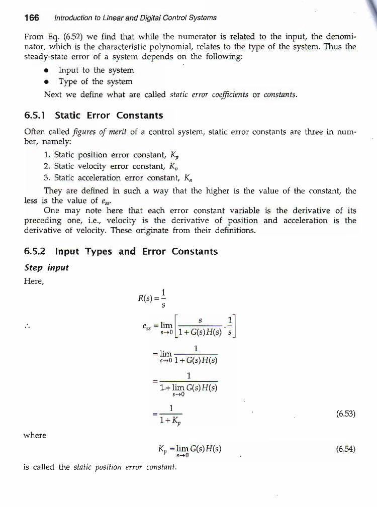
6.5.2 Input Types and Error ConstantsStep inputHere,

R(') = 15

. t s 1l.. c-=Slr_qu*o 1

.. 1

"-,0 1+ G(s)H(s)

L+li4G(rHG)

11+K"

where

Kp =lt4GG)HG)

is called the static position error constanl.

(6.53)

(6.54)

l//'

RamP inPut

tlete,

Tme Domain Peiotmance ol Conttotsystems 167

1RG)=-

I s 1l""=SL*cG)At 7l

1- li'n-

ijd st1 + GG) H(s)l

1-limsG(s)H(s)

s+0

1 (6.5s)=K"

where(- = lim sG(s)H(s) (6'56)

is called the static oelocity effor constdnt' We note that ii co:tair-rs an s which indicates

differentiation for once rn t"*""ari;';tflt til fact thai velocity is the fusi derivahve

of the position variable'

Parabotic inPut

Here, 1

R(s) =-s-

| " 1l- - l i ' - I

- . - l

" _ y-i [1 1c1gHG) c .l

1- l i s-

;lt rtlr + c(s) riG)l1

- lim s'?G(s)HG)

1 (6.s4Ko

whereK- = lim s2cG)HG)

(brd)

' ' arhich indicates a sec-is called the statb acceleration conslaflt' Ptediclably' it contans s- '

J.J-d"rlttuti.t" of the Position vadable'

I168 Introduction to Linear and Digital Contol Systems

6.5.3 system Types and Steady-state Errors I

Y"_1,:9:.0.,1n" try." 9l " system_ earlier (Section 2.11). Ir is determined by the numberor pores af the oflgrn (i.e. at s = 0) ̂ exis.trng in the openJoop transfer func'tiorL G(s)H(s),of a system. The general form of G(s)H(si is

'

c(s) H(s) _ {(1 - sTrXl + sTz) ... (1 + sI", )' '

s ( ( l - s4)( t +sTr) . . . ( t +s7l )In Eq. (6.59), k is the number of poles at the odgin. Therefore, it $ a type k svstem,EXAMPLE 6.13 Identify the t]?e of the system for which

^ , , K( ] +3s) j -5s( r l D r 1 - a l l o E l S l = -

s ' s '+6s+7

c(s) H(s) = {++ls)gjjj.ls ' (s " +6s+7)

Solution: Here,

(6.se)

(6.@)

Since the number of poles at the origin is 2 (indicated by s2 in the denominator),twe = 2.EXAMPLE 6.14 ldentify the t'?e of the system for which

C(.) =-,-- j _ and H(s.1 = 5.3s-+bs+/

Solution: Here,

c(s) H(s) = -4(s - 3)

s '+6s+7

It has no poles at the origin. Therefore, irye = 0.

. .With this background, we see how the static erlor constants, and for that matter,steady-state errors are related to t)?es of systems.Type O

Here,

C{s)H(s) _ K(1 + .7r Xt .s I2) . . . ( t + s i ; , r(r + s4 xt+ s4). . .(1 - s4)

Ko =lu1c(s)H(s) = K'1-1 J=7i

11%"= r+ Kp= 1+K 661)

7. Step input

/

/ z. r-*p irrput

fnne Domain Peiormance ot conjtrotsystems 169

3. Paflbolic inqut

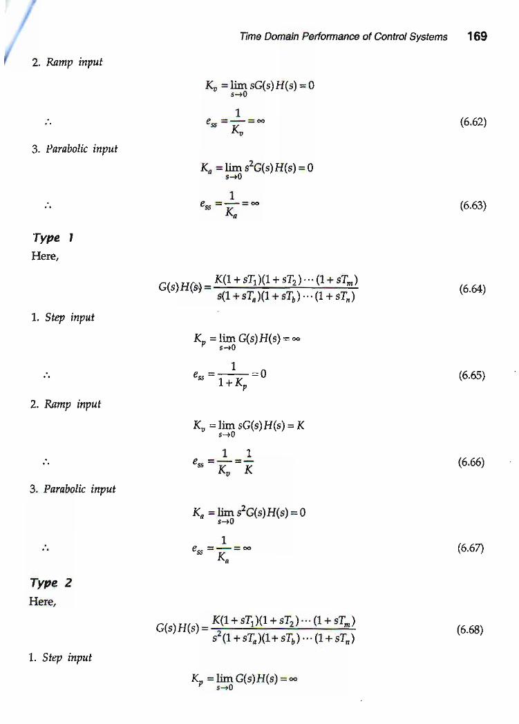
Type ,Here,

7. SW input

2. Rntttp input

3. Pffinbolic input

Type 2l{erc,

K, = l imsc(s)H(s)=0- s-ro

1

K- = Iim s2c(s)H(s) = 0

.r . \ , {n\ _ K( l+sT1X1+ 5T2) (1+sT")

s(1+ s4)(1+ sTr) " (1 + si;)

Kp =lil4GG)HG)=-

1^e5s =""--=U

K" = lim sG(s)H(s) = K' 6-i0

11ess=17=A

K- = lim s2c(s)H(s) = 0

1

^. . . , , . K( l + sTlx l + sTr) " (1+sTn)u(srrI (5, = -.;----=i;:---=1----;-:-;-

s ' ( l + s l4xI+ srb) ( r+sr t r ,

& = l imG(s)H(s)=-' s '0

6.4\

(6.63)

(6.64)

(6.65)

(6.65)

$.6n

1. Step inp t

(6.58)

179 lnfuuction to Lineat and Digital Control Systems

.'. e" =-1.=or+q=" 6.6e)

2. Rmnp input

K, = lim ;c(s)H(s) = -_ s ' 0

1^e"" =;- = U

3. Pqrq.boli input

(6.70)

& =lrms'?cG)ruG)=r

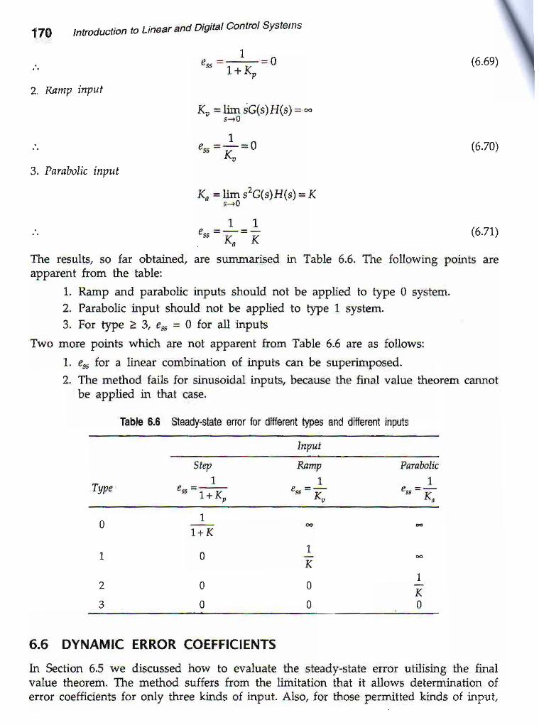
. %=K=" 6 .71)The results, so far obtained, are summarised in Table 6.6. The following points areapparent from the table:

1. Ramp and parabolic inputs should not be applied to t)?e 0 system.2. Parabolic input should not be applied to [pe 1 systern.3. For t)?e 2 3, eu = 0 for all inputs

Two more points which are not apparent from Table 6.6 are as follows:1. e* for a linear combination of inputs can be superimposed.2. The rnethod fails for sinusoidal inputs, because the final value lheorem camotbe applied in that case.

Table 6.6 Steady_slale effor for ditferent hpes and differsnt inDuts

WlttStep Rnnp Parabolic

1IWe e" =:---:- e__ =_ll +^ , - K "

1+K

0

0

0

6.6 DYNAMIC ERROR COEFFICIENTSbr Section 6.5 we discussed how to evaluate-.the steady-state error utilising the finalvalue theorem The method suffers from the limitation

'th"i ii

"-d*r determination oferlor coefficients for only tfuee kinds of input. Also, for those permitted kinds of input,

1K0

1K

0

0

l-tme Donain Peiomance of controt systems 171

it does not show how the error varies with tirne' These disadvantages can be overcome

uy fo owing the method of finding generalised error coefficients that are often telmed

dvnamic error coefficients.' The eror function, we iound in Eq. (6.51), is given by

E(s) 1R(')

= 1+ GG)HG)

The denominator on the right hand side of the equation is a function of s

be written as powe! series in s as follows

E(s) 1 . 1- ,7^2,R(r)=&-i<t" '8"

- '

EG)=:RG) ++sn(o +l lKsr+..K1 l(2 ^3

The inverse Laplace transform of Eq. (6.73) ytelds

<n = {,<t. {*,<tt + {ft ,o * "' (6.74)

GG)HG) = KG+4)s(s3+5s2+6s)

find (a) type of the system, (b) static error constants and (c) error due to input fr2

'

Solution:(( '+L\ - - {G+4) . Therefore, we =2.(") GG)HG)=d;i ;6o s,(s, +5s+6)

(b) Since it is a type 2 system, 19 = K, = *.

K, = lim s2c(s)H(s) =tl^:!:'9-=2:' ' s+0 seus -+5s+b J

(c) The input is parabolic. Its LaPlace transform i" RG)=4'

A3A2K

(6.72)

and it can

(6.73)

Ttrerefore, if the input function is known, dynamic error coefficients can be figured out

throueh a compatison between Eq. (6.7a) and the polynomial obtained from invelse

Laplaie transfoim3. The following Lxamples will make the procedure clear'

EXAiIPLE 6.15 For a system having

Therefore,

lSome authors define e or coefficimts as Ci = I/Ki.

'qil172 tntroduction to Linear and Agihl Control Systams nt

EXAIIPIE 6.tG The open-loop transfer function of a servo system with unity feedback isgiven by

500L,(s.f =;I+0_;i

(a) Evaluate the error series of the systen.(b) Deterrrine the steady-state error of the systen for the inpui t(t) = L a 21 * ,2.

Solutlon: Since it is a unity feedback syster; we have

E(s) 1 s+0.1s2R(t=1.cO=sofi;nI'

The long division of the right-hand side of the equation yields

0.002s + 0.000196s2 - 0.000000792tr

500+s+0.1s2 ) s + 0 .1s2ts-r 0.002s2'a 0.0002.s3

0.098s2 - 0.0002dt0.098d i 0.000195s3 i 0.0000196/

-{.000396,s3 - 0.0000195#

+0.000396d r 0.000000792d + ...

E(s) = o.oozs + 0.000196s2 - 0.000000792s3 +...R(s)

E(s) = 9.002t41r1 + 0.000196s2R(s) - 0.000000792fR(s) +

= a ^G) n] r^Gy + =1- s'zn1s1 + ] sanlsy +..'Kt . , Kz

. , K3 " K4

Its invelse Laplace transform Felds

tt,tt\ ,l2r(r\ i3t,'\e(t) = $W2;! + 0.000196 :i+ - 0.00r00ffi792 :-:* + ..

We are given, r(r) = 1 + 2, + t2. Therefdre,

dr( t) =z*2tdt

d3r(tl ^--:-i- = udt'

TirE Dolain Pettomane d contd systr'ms 173

These give

e{t) = o.oa2? + 24 + 0'000196(2) - 0'000000792(0) + "'

= 0.004392 + 0.004,

{a) The eror series of the qrstem is e(l) = 0'00'1392 + 0'004t and the dynamic error

coefficients are

Kr =1=-0

x' =;l==596' 0.002

Kr =:*- = 5102'04' 0.0001%

K ̂ = - ==: *= = - 12626:26 26' 0.000000792

O) The steady-state eror in time-domain is

lim e(t) = lim (0 00439 + 0'004t) = -tr- lJ-

EXAIIPLE 6,17 The opea-loop trarsfer function of a unity feedback system is glven by

G(s)= .4=sls + ru,

Find out dynamic error coefficients and the error series when the inPut is r(t) = 1 + 2t

+* .

Solutlon: It being a unity feedback system, we have

E(s) 10s + s2RG)=50-10;7-

Note that since we want to find out a polynomiat in ascending powers of s' we

have to arrange the numerator and denom:natoi in that order, before Performing the

long division' By long divisiorr we get

E(s) = 925p1t1 - 0'02s2R(s) + (o)CRG) + 0'004#R(s) + -

Its inverse Laplace transform yields

trt t \ ,12,1t\ A3 l \ dar, l . le?r=@\r(t\ +02!y - o.o2 ":i)'/ +(0) " j:i' + 0'004:-:j:' + '

dt dt' dt' dt'

=*n .t#.*#.;#.+#.

174 lntroduction b Linear and Digttat ContlOf Systerns

Drrarrric error coelficimts are, therefore,

& =1=-0

r, =;1.=5

",=-#=-*rn =]=-

0

*G='fo=_The input is r(t) = 1 + 2t + *. 9o,

i t \:::):! =2+ 2t

d2r(t) ^dt'

Thus the error series is given by

4t)=o.2(2+2r-0.02(21= 0.36 + 0.4t

EXAITPIE 6.18 The open-loop hansfer function of a unity feedback system is given by

c1t1=-"---. jP' s'(s + 4xt' + 5s + 25)

l-l"ni:t"::';Fnirldrf; o*ar*tat" error of the svstem when it is subjected

Solutlon: Static error coeffici€nts are

& = lim GG)HG) = tg a,."a, *g-,. *, = -

K" = lim sc{4'(s) = ga,.4# u" - *) =-

&=tims'zc(s)H(s)=u-, loo = 10 =ts+o sro (s + 4Xs, + 5r + 25) (4X25)

Taling the Laplace transform of the input, we get

) L A .R(s)=:1- :a -

5s_s"

rWe obsewe that

the steady-state error

Time Domain Performance of ContralSystems 175

this is a combination of step, ramp and parabolic inputs. Henceis given by

=lim

, -= 2

*4 *4" 1+ Kp K, ("

Substituting the values obtained for the error coefficients, we get

,"=j-*a *!=+

EXAMPLE 6.19 A servomechanism, the block diagram of which is given in Figure 6.17,is designed to keep a radar antenna pointed at a llying aeroplane. If the aeroplane isflying with a velocity of 600 km/h, at a range of 2 km, and the maxirnum tracking elloris to be within 0.1o, determine the required velocity error coefficient.

Sofution: Giver; the velocity = 600 km/h ='166.67 m/s. The radial dGtance = 2km= 2000 m. Therefore, the angular velocity is

u 166.fio = - = --::+ = 0.083 rad / s = 4.756 desJ s

r 20ffi

The input to the hacking system is the angle swept in time t sec. So,

r ( t )=at=4.756t

+ RG)=!iq

The open-loop trarufer function of the system is

G(stHrs) = K'' ' s(1+ sT)

<r1 r <?\ r L1 + G(s) HG) = :-:-l-:j-1-:jr

s (1+s i )

Thus, the steady-state error is given by

&

Figure 6,17 Block diagram of servomechanism (Example 6.19).

s,o 1+ G(s)H(s)

176 tntrcduction to Linear and Digital Control Systems

. . 4.756 s(1 + sT)s+0 s ' S ( r+s l ) f I \ z

4.7ffiK.

To maintain steady-state tracking erlor at 0.1o,

4.756 ^ "K1

or K' = 47'56/s

EXAIIPLE 5,20 Find tyPe, error coefficients and eo for the system, shown in Figure 6'18,

for the inputs (a) r(t) = 12, (b) 7(t) = 6r and (c) r(t) = 12 + ot + l*'2

"-t.l = --- 2-- ' ' - ' (s+sxs+10)

H(s) = 55

Figure 6.18 Block diagram lor the cofirol system (Example 6.m)

Solution: The block diagram can be reduced to give Figure 5'19'

Flgure 6,19 Beduced block diagram (Exanple 6.20).

rTherefore, the open-loop tmrsfer function of the system is

10c. 250 250cc) H(s) =

| -eHl = (r- t/G' r0)- rrsr

=; - t40r - 50

It has no poles at the odgin. Therefore, it ls a t,?e g sygtem For a t)?e 0 system' only

the static position error coefficient, Kp, exists, its value being

,q0Kp = lim c(s)H(s) =

l* 7; = s

Time Domain Performance of coni{.olsystems 177

Therefore,

- . sR(s) 72P = l r m-"

*d 1 + G(s)H(s) 1+ Kp

Therefore,

, = l ; r n 5 = --s

s -tj s[1+ G(tH(s)]

- . . L2 6 LK(s)=-+-+-

s s- zs-

Since erors for individual inputs can be superimposed and we have aheady seen that

"" l"t tf-," second Part is -, wlthout calculathg it for the third Par:t we can say that for

this input also e," = -

EXAITPLE 6.21 Determine the range of values of K of the system shown in Figure 6'20

so that es < 0.004 when r(t) = 0'2t-

_ . . 12(a) Here, l<(s) = -

O) Here, R(s1={

(c) Here,

Solution: The

Here,

Figure 6.20 Control system (Example 621)

open-loop transfer function for the system is

KG(s)H($ = ^

rt! f r./

s (s+1)+Kl-CG)H(s)=-

t\r T r./

t(t) = 0'2t

- 02K(s) = --5-

178 lntoduction to Linear and Digital Contot Systems

Therefore,

e*= j inr - - * ] : -sro 1+ c(s)H(s)

=umlo;2 : 'G+1) Is - 0 1 a . . . t c L v l

,. 0.2(5 + t)- |Ur _-i-

s ros -+s+K

o.2(

From the given condition

0.2--=K

< 0.004

.. 0.20.004

K>50

6.7 EFFECTS OF ADDITION OF POLES AND ZEROS ON RESPONSE OFSYSTEMS

]: : .t"=Tg to. study the effects of addition of poles and zeros on response ofsystems. While doing thal we will restrict ourselrres' io

-"".onJ ora", underdamped

:I^tj:ff_Td. r*p.tesgonsg on! t"q,,"ys,"* .url U-" ,"p."r"rrt"a by their open_loop orciosed-ioop hansfer functions. We will coruider bo& separately- The other 'urro*p.tio"

is that poles and zeros wil be locared ," th" dft_ili';;J} "^_ro""".

6.7.1 Addition of poles

As told earlier, this studv can be made-on open_loop and closed_loop tralsfer functions.:t""T*"

*" srudy meaningtut, *e "on

conliae. uiiq, i""-Ju".i'iy,"*" for openJoop

Closedloop transfer functionLet the closed-loop transfer function be

Obviously it is a second order.system with q = 1 and f = 0.3. We add a pole to make

1rI (sJ = -a-. -

s '+ 0-6s+1 r r 's+1

(6.75)TG) =-"----:-s '+0.6s+1

(6.76)

ii'Figorc 6'212ar .d4

Time Damain Peioman@ ot control systems 179

shows step responses for the system represented by Eq. (6.75) lor ro = 6, 1,

1

0.8

0.6

0.4

0.2

00 2 4 6 8 l0 12 14 16 l8 20

_---__-_________>, (s)

Figure 6.21 Step responses for Eq. (6.75).

Here, we obsewe that as ?p increases, rise time increases, but peak overshoot decreases.We add, though observed in a Particular case, the conclusion is general.

open-loop trdnsfer functionLet the oDen-loop transfer furction be

G(s)=--1-D\' T Z,/

We add a pole at s = - a to make it' t p

4t\ r.4

1l"

(6.n)

s(s + 2)(1 + ros)

feedback closedloop transfer

c(s)i ( s l = -" 1+G(s)

1

The coresponding unity

. / . r ? \ r 1 + r < \ + 1! \ , , _ t \ _ - p t , i \

function is

(6.78)

180 Introduction to Linear and Digitat Control Systems

,,*rJ1lr.tt"o responses of Eq' (6 78) corresponding to 6 = 0, 1,2 a d 4 are plonec

tu tz 14 16 lt 20

Figure 6,22 step responses for Eq. (6.78). --"-------' t(s)

It -may

te^observed from this plot that 1s g ircreases, both peak overshoot and dse timemcrease. An increase of a means that the fob comei "for"i

io tf,u o"g_ in the s_plane.The conclusion, though <irawn for a particular """",

i, i" J;l ;;tte generat.

6.7.2 Addition of ZerosAs in the case of poles, here also..we will consider open-loop ard closed_loop casesseparatety and a unity feedback will U" .o.siae..a-]oi.ie ;;:#"p.Closedloop transfer functionLet the closedloop transfer function be

1r (s, = ;r_:_::;

We add a zero to it at s = _1/r. so that

7+ t_sI (S) = --:-----j--

s '+ s+ 1

4t) 1.5tII

(6.7e)

(6.80)

fime Domain Peiormance ot Controtsystems 181

Equation (6'80) can be written as

1 1

T(s) = ---:---= * ""s

- , -s '+s+1

- s '+s+1

So, if c(t) is the step response of Eq- (6.i9), that of Eq' (6'81) will be

c^(tl=c(t\+r, .Lc(t)' - d t

Figure 6.23 shows the Ploi of c(f), t.!c$) and cg(r) It is clear lrom the figure- d t

that the zero term decreases the rise time but increases the Peak overshoot'

(6.81)

(6.82)

I 12II9 re

6

0.6

0.4

0.2

0

4.20123

-_______) I (s)

Figure 6.23 Efiect ot addilion of zero to closedloop transier tunction'

OpenJoop transfer functionLet the open-loop trarsfer frmctioa be

1G(s, = -_-s(s + r,

and the zero a1 5 = -1/t. Then the unity feedback closedloop iransfer funetion becomes

7+ c-sT( <\ = ---------:-- ' ' '

(1+t s )+s(s+1)

(6.83)

(6.84)

182 lntroduction to Linear and Digital Contrcl Systems

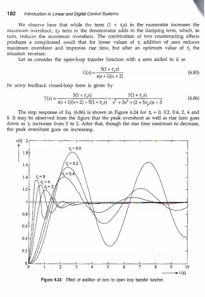
We obsewe here that while the term (1 + z-s) inma\imum overshoot, r:) term in the denominator aJds totum, reduces the maximum overshoot. The combinationproduces a complicated result that for lower values ofmaximum overshoot and irnproves dse time, but aftetsituation reverses.

Let us consider the openJoop

the numerator increases thethe damping term, which, inof two counteracting effectst: addition of zero reduces

an optimum value of ?, the

(6.8s)G(s) =5(1+ r"s)

s(s+1Xs+2)

Its urLity feedback closedJoopform is given by

transfer function with a zero added to it as

__>, (s)

open loop lransfer iunciion.

(6.86)s(5 r l l (s -2) 5(1 - r .s ) s r +3s2+(2+5rrs)s

"5The step response of Eq. (6.86) is shown in Figt,re 6.24 lor t = g,0.2,0.4,2,4 a d

8. It may be obsewed- from the figure that the peak overshoot as well as rise time goesdown as ?, ircreases fiom 0 to 2. After that, though the rise hme continues to decr&se,the peak overshoot goes on increasing.

c0

I

0.8

0.6

0.4

o.2

Figure 6,24 Effect 0f addition 0f zero to

fime Domain Petormance of Contrcl Systems 183

The results of addition of poles and zeios are summarised in Table 6 7'

Table 6,7 Sumrnary of effects of addilion of poles and zeros

As the PoIe fiearc Lhe origtn As the zero nears tJle origin

Type of tnrsferfurrction

Rige tu e

t l

Peak o7)ershootM.

Rise timetl

Peak ooelshootMP

Open-looP

Closed-looP

Decreases up to ace*ain value of t butincreases thereafter

Increases

lncteases

Increases

lncreases

Decreases

Decteases

Decreases

6.8 MINIMUM AND NON-MINIMUM PHASE SYSTEMS

In section 2.14, we had talked about minimum and non-minimum Phase systems' HeIe'

;";;;;',; see the dirterence.:j :T"?:*'*i:':::; il:"'il:",tiil, in rheir rransrer

We recall, minimum Phasefur.;"r. i;t# ,yr,"- i" oi.o.--iri*l.- phase, the sweep.in phase area is larger' Let

us compare the unit steP lesporues of minirnum and non-minirnum phase systems' the

"--rr?.'run.no* of which are given by

c(4 = 6-"1'; =

the unit steP

- (+ l

;! 'a =c",**,ts)=;--x(s)

response of the sYstems in Figure

1.4

1 .2

0.2

0 6Time (s)

-n----"--s" +s+1

(6.87)

(6.88)

6.25 and Figrrre 6.26

and

We presentrespectivelY.

1

E 0.8

E 0.6

0.4

12l0

Figure 6.25 Unii step response of a mlnlmum pnase sy$em'

1A4 lntroduction to Linear and Digitat Contot Systems

1.4

1.2

I

0.8

0.6

0.4

0.2

0

4.2

r'od

'"lffii,',,i,,'i;'.'[3,:','J.'fff ' ; ;frT",fr:um::;fiil;,il l,:li''l*'. The difference in behaviour ig',1-4df ;]1#ll1llilJlifl l,*"1,flffi ':,,,1hlj*:l;trfiilf j,T:

t2l0

lEYlEw Qurslor.rs1, Choose the correct artswer:

"' T".Hff:'ff;Tation or a svstem is s2 + 2s +2 = 0. rhe sysrem is

riiii """,i",i.pi1"'* .1_-'j :3:.oTo"o@1 ror a controi f1"m to be ,

ttt' none of these

oampng ratio should be JPerated in overdamped conditiory the value of the

(i) 0(iii) 1

(ii) > 1

(c) The steady-state error for a (iv) < 1

(i) zero tPe 3 sy-s.tem for a unit step input is

(iii) one .$l ffH,t(d) The open loop transfer function of a system is l0 . *o ",due to a unit step input is

-'- 1+t

rrre sready-state error

(i) 10

, . . . ' 1{r1l l -'11

the final value is

(i) 1.2 s(iii) 2 s

(i) increases dse time(iii) increases ovelshoot

l1me Domain Pefiomance of Control Systems 185

(ii) 0

(iv) -

(ii) 1.6 s(iv) 0.4 s

(ii) decreases rise time(iv) has no effect

(e) The second order system defined by the transfer f,-.t." ffi

= - . 3 * "

given a unit step inPut. The time taken for the output to settle within i2% of

(0 Addition of a Pole to the closed-loop transfer function

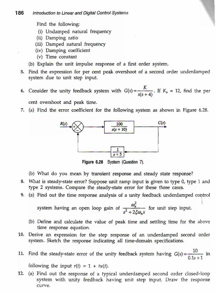
2. Corsider the block diagram given in Figure 6 27'

(4,

(b)(c)

3' (a)

Flgure 6.27 Block diagram (Question 2).

Find the closed looP tlansfer tunction T(s) = YG)/RG)'

Find the CL unit steP resPonse.

Find the final value of Y(t).A first order system when subiected to a steP inPut has a lemPerature nse

of 25'C after an hour and 37.5'C after 2 hours, sta*ing from coid condition'

Calculate the final steady temPerature rise ard the thermal time constant'

Sketch the timedomain response of a tyPical underdamped second order sys-

tem to a step input. On this sketch, indicate the {ollowing:

(i) Maximum peak overshoot, Mo(ii) Rise time, t,(iii) Delay time, l;(iv) Settling time. ts(v) Steady-state eror, e.s

4. (a) A second order differential equation is given by

(b)

d2x -dx - --"=* 5":- ' l /x = /Vd td t '

186 lntroduction b Linear and Digitat Control Systems

Find ihe following:

9.

(i) Undamped natural frequency(ii) Darnping rabo

(nf Darnped natural frequQncy(iv) Damping coefficient(v) Time constant

(b) Explain the unit impulse response of a first order systen.

fin9 the, expression for per cent peal overshoot of a second order underdampedsystem due to unit st? input_

Coruider the unity feedback system with GC)=- I( ^ . ff K. = tZ, find the per

cent overshoot and peak time.(a) Find the error coefficient for the following system as shown in Fizure 6.2g.

Figure 6.28 Sysiern (euestion 4.

(b) I fhat do you mean by transient response and steady state response?What is steady-siate error? Suppose unit ramp inpnt is given to type O type f *atype 2 systems. Compare thJ iteady-state error lor ttre-se three iises.(a) Find out the tirne response anaiysis of a unity feedback urderdamped control

system having an open loop C* " T#€r,,

for urdt step input.

(b) Define and calculate the value of peak time and settling time for the abovetime response equatiot.Derive an expression for the step response of al underdamped second ordersystem. Sketch the resporue indic;fing ;U tirne_doqrain ;;".id;;*.

Find the steady.5late error ol the unity feedback system having C1s;=, :10 . in' - 0 .1s + 1

following the input r(t) = l + tu(t).(a) Find out the response of a tlpical underdamped second order closed_loopsystem with unity feedback having unit st+ input. D.aw the responsecurve.

72.

llme Domain Perfomance of Control Systems 187

(b) A unity feedback second order servo s)'stem has Poles at -1 ! j2 a d zerc at

-1 ! 10. Its steady-state outPut for a unit step hPut is : ' Determine the

transfer function.

19. (a) Sketch the unit steP response of a second order system indicating Peak over-

shoot, dse tilare and settling time.

(b) A temPerature sensing device can be modelled as a fust order s)slem with,a'

time constant of 6 s. Ii is suddeniy subiected to a steP inPut of 30'C to 150'C'

What temPerature will be indicated in 10 s after the process has started?

14. (a) Define the fouowing:(i) Rise time (ii) Delay time

(ni) Settling time (iv) Overshoot

(b) The open-loop transfer function of a uaity feedback control system is given by

AG(t )=r (1*r r )

(i) By what factor should the amplifier gain A be multiplied so that the

dimping ratio is inceased from a value of 0'2 to 0'6'r

(ii) By what factor should amplifier gain be muJti,plied -so- that the overshoot

oi ttt" ,rLlt step resPonse is reduced ftom 80V' to 209? [% overshoot =

r"-----'=100 exP en|/^11- 62I, d = damping ratiol

15. (a) Find out the resPonse of a typical underda:nped second order closed-loop

system with unity feedback having steP inPut'

(b) For a unity feedback closed-loop control system, the open-loop transfer

function is given bY' E

..(s,r=;G;5

Calculate the value of rise time (t') and maxiqrum overshoot (Mo) when the

system is subiected to a unity step inPut'

16. Write short notes on the following:(a) Time constant(b) Settling tirne(c) Peak overshoot(d) Standard test signals used in time'domain analysis of control systems'

BASICS OF CONTROLLERS

7.1 INTRODUCTION

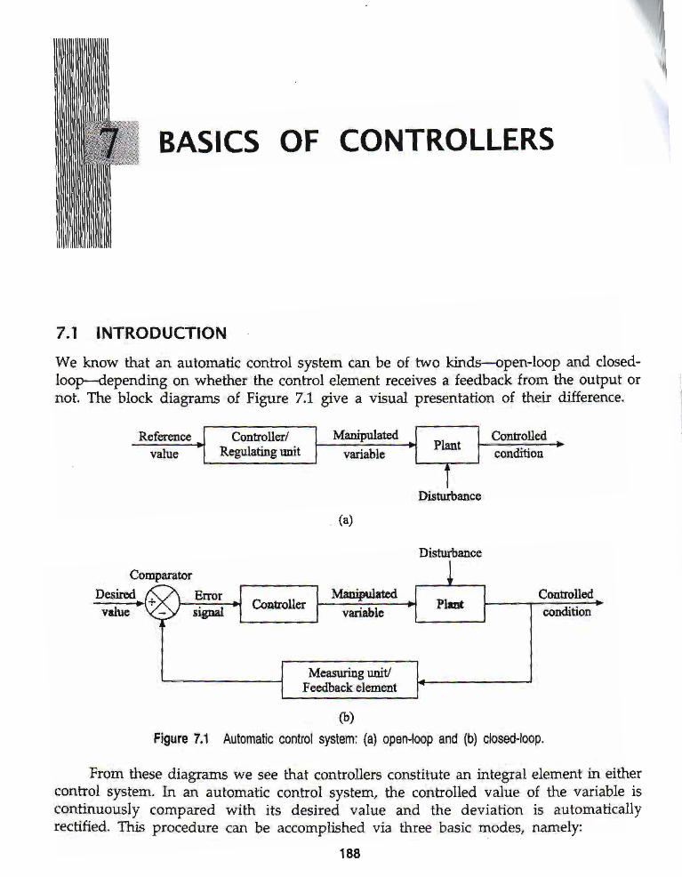
3" h9* that an automatic cont(l".",Hi',",HT;##t;iH;.]i{:rfi "ffi ff ":jff #Fi"#"{'T#i:"{lt:;

Disturt ac6CoEpaaatoaDcsirEdyrlue MaiF&red

Cotrtoll€d

Figurc 7,1 Automatic &)

conrot system: (a) openloop and (b) closeoroop.

fl*;,*ftd,#$$i1**ld**$,ffi 't"ff .:*tjtr188

Basics of Contrclters 189

1. ProPortional2. Inte$ar

i"ffi i!'x*T":'.i:1"" :ii:"T"ff ,f; iJ-h?1":':1d".",:J'S""Jiil;rharacteristics So' controllers can oe urvruEu

on their mode ot contror:

t. Two-posifion or ON-OFF controUer

2. ProPortional (P) cortrouer

3 InteFal (I) controller --.4 Dedvative (D) controller

i. proo-tio"uf Plus inte$al (PT) conholler

i. i""i"tn*"f plus derivative (PD) controller--.

i. or"'p-,t"rr"l ptus integral plus derivative (PID) controuer

h the fouowing sections we will consider these controllers and evaluate their

perfolmance'

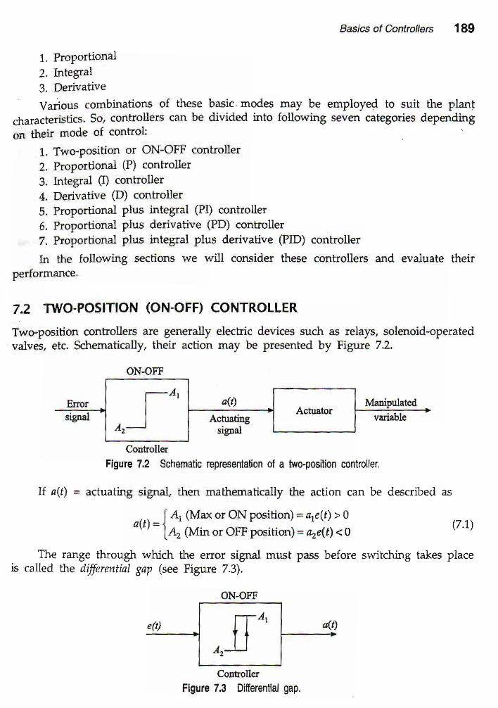
7.2 Two-POSlTloN (oN-oFF) CONTROLLER

rwo-position contr?Tl,:.:':,i:.^::',Lv^ "i":xx"?:::il:1;i,'$ll";;:'*"'o-operatedvalvel, etc. Schematicary' theu a

Contoll€r

Figure ?'2 Schematic representaiion ol a lwo-posftion controller'

d(t) = actuating signal, tJnen mathematically the actron carr

I A, (Max or ON Position) = ale(t) > 0a(r) =

la, 1r',,tin or oFF Position) = nze(r) < 0

The range through which he error signal must Pass before switching

, iii u""ai6rrrrrit gaP bee Figue 7'3)'

be described as

(7.1)

takes place

CoDfroller

Figure 7.3 Differential gap'

ON-OFF

--4,

IAz-

ON.OFF

190 lntroduction to Lineat and Digital Control Systems

The advartages and disadvantages of this t'?e of control are ljsted in Table

Table 7.1 Advantages and disadvantages of on-ofi controller

Adoahtage Disadaantage

Simple, economical. Used in domesticapplances as well as in industry where roughcontrol t5 necessary_

Transient conditions and steady-state accu-racy a.re not much improved.Controller condition oscillates around theset point.

1 .

2.

7.3 PROPORTIONAL (P) CONTROLLERIn a proportional controller, the actuating signal is proportional to theMathematicalln if ri(f) = 6gtu6tin, signal, the;

a{t) e e(t)

= Kf(t)

e[or signal.

(7.2)

(7.3)

The Laplace transform of Eq. (7.2) is

Here, with the

Figure 7.4 Second order system.

proportional controller

K r,fGG\HG!=

" P-'' ' s (s + 2€a4\

sR(s)" , -o1+c(s)H(s)

,aG) = I(pEG)

I^n:l: *l b called the controller gain. Though generally its value is greater than 1, it canoe ress rnan I ln some applications. Since in most of the cases ii ampJifies the errorsignal, it facilitates deteiti-on of small deviations and its eventuat remedy by theactuator.

7.3.1 Accuracy

Consider, for example, the second ord.er system given in Figure 7.4.

Therefore,

addition of a

/

Basics ot Conttolle6 191

=lim

input

RamP inPut

In this case,

Parabolic inPut

ln the case of ParaboUc inPut'

- r , * t ' ( t *26 ' " ) ^ .R(r )- iii s(s + 24a,) + Kvroi

(7.4)

sR(s)K"o;

'1 -L- s(s +2€ot )

StePHere,

- - , , ' - t ' ( t * 26 ' " ) = .R(r )""

- i36 s15 +260t"1+ Xrto;

szG +2{to,1 1- l i n ; . --

iI6 s9+z€a,l + Kpai s

s(s + 21a"\- 116 ------'------.7-

iI6 s1s + 2(a,) + Kra4-o

.. sR(s)'" - li 1+ GG)HG)

-r .^ s2 (s + 2€a, ) - .1-- ?)d 52 a2s6x1, + Kp(Di s'

Kpa,

(7.s)

(7.7)

(7.6)

_, ._ sR(s)- ;6 1+c(tHG)

_r.^ s2(s +2€ot , ) " .L=*-

il6 sz + 2s€a^ + Kptt s"

7.3.2 Advantages

The following are the advantages of proportional controllers:

1. This tyPe of controller *t'"*"' *t io*artl Path gain ^We

have seen in Eq (5'20)

that an increase t tn" 'otiiutJ p"tft g"nt increases the undamped natural

192 tntrcduction to Lineat and Digitat Contol Systems

fl".1T::r,":L-**1..1,y1, ,*d*:s the damping rario {. so, the resl,if;n:: J:ffi "l::, ::::s:Tni.;'::tT"'J:-i:!:r:';j:::'i:' ffi '';.:1';lwjlT::.1-.1":" * jncr:asd pe"i o,,e.shoot ,h;;sh ;;ffis.;.'; H:Tlil, ;"",f ;""1';:l; iT.:.tT ,l1i1*: of contro'er, { .1 ;-;; ",l, ,,?*'ff.""^B: *g:l j; ,.':,*" fl :';[ "p {#;i; :s ;:"*:":] ; J ,*' ;,T,::J"ilif K, is too high.$,;.i.T';.T:""i K, irn pr ies i";;,'{;;; ;;il,li ;:;?tr;',# ;ystem u$table

3. It is a stable control as long as (, is not high.

7.3.3 DisadvantagesThe following are the disad.vantages ol proportional controllers:t

fi"%Tl.*"yil::rroller causes offset, i.e., it may cause a sustamed deviarion from2. It increases the maximum overshoot of the system because it lowers t

7.3.4 Realisation

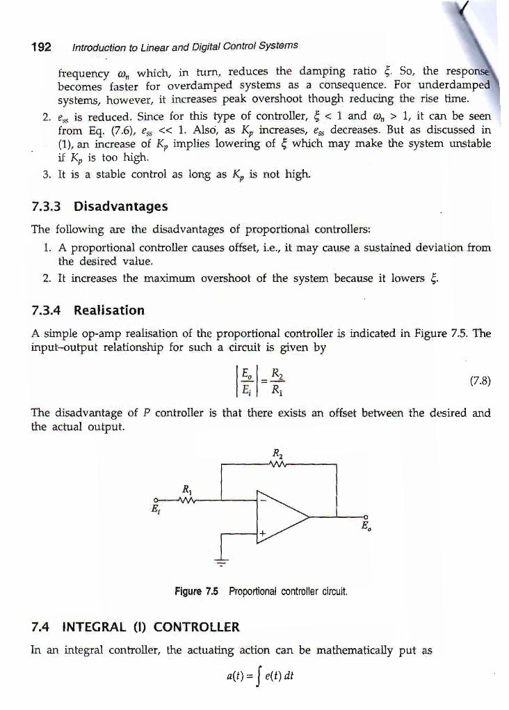
A simple op-arnp realisation of thrinput-output *tu"*l,+^1", "*i :':i*if;:iloller

is indicated in Figure 7.5. rhe

(7.8)

ft" iil:ltff#:i or P controller is thar there exists an offset berween rhe desired and

Figure 7.5 proportional mntroller chcujt.

7.4 INTEGML O) CONTROLL€R[:r an integral controller, the achratrng action can be mathematically put as

a@=Ie\dt

r, I n,E, I Rt

=x,le@dt

Basi6 ot controtleg 193

(7.e)

(7.10)

(7.73)

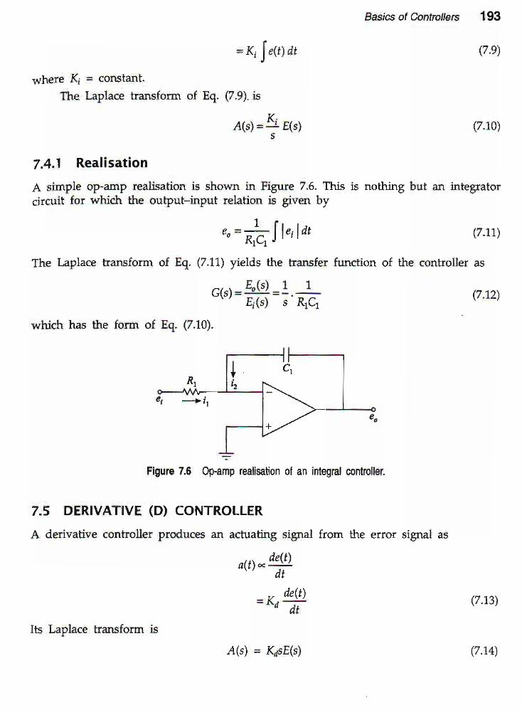
7.4.1 Realisation

A simple oP-amP realisation is shown in Figure 7 6' This i5 nothing but an integrator

clrcuit'for which the outPut-input relation is given by

,"=]7l1,,, lat (7.r1)

TheLaplacetralsformofEq.(7.11)yieldsthetralsfelfrmctionofthecontlol]eras

61r.1= E"(t) =1. -1= (7.12)-' ' ' E;(s) s R1C1

which has the form of Eq. (7.10).

where Ki = constant'

The Laplace transform of Eq. (7.9) is

AG)=!-E(s)5

7.5 DERIVATIVE (D) CONTROLLER

A dedvative controller produces an actuating signal from the enor signal as

... de(t\alt ) * ---1;-

a t

=K,t9'dt

Its Laplace transform is

AG) = KasEG)

Figure 7.6 Op{mp realisation ot an integral contlollet

(7.74)

(Figure 7.7) of a derivative controlieroutput is rclated to the input as

dr.e" =RC+

a t

From the Laplace transform of Eq. (7.1,5), we get the transfer funcnon

c1s1= &(d = ,tat,(s)

7,5.2 Advantages and DisadvantagesAlso called tl\e rate controlltr, a dedvative controller improves thethe system. The djsadvantages, however, are many:

1. It amplifies the noise signal.2. It may cause saturation effect in the actuator.3. It does not impiove e"" because of generation ol a zero in

_ The disadvartages of a derivative controller far outweish thethat it offers. That is why it is neaer used alone.

194 lntroduction to Linear and Digital Control Systems

7.5.1 Real isat ion

The simple op-amp realisationa differentiator for which the

7.6 PROPORTIONAL PLUS INTEGML (PI) CONTROLLERbr the case of a PI controller,

a(t) = Kre(t) + K, Je() dt

i , t a - 1

is nothing else thajl

(7.1s)

(7.16t

transient response of

the hansfer function.only one advantage

(7.17)

{7.18)

I

Figure 7.7 Derivative controller.

at'l=[r-'f)er"r

7.6,1 Control Action

The achJating action of a PI controller for erlor inPut of a unit steP can be worked out

from Eg. (7'18) asf t -

a(t) = Kou(t) + K; Jo

r(t) dt = ̂ p + ̂ ir

Basics ot Conttollets 195

(7.1e)

Thus a step error signal will produce a ramp actuating signal as shown in Figure 7 8'

7.6.2 StabilitY

To check the stabiUty of a PI controller' let us consider a second order closed-loop

;;;l; *r,i.n rt ij attached (see Figure 79)'

d(t)

t

Figure 7.8 Actuating signal of Pl conro er for step error input'

Figure 7.9 Pl c'onlroller attached to second order pianl'

195 lntodltction to Linear and DigitalControl Sysbms

The overall transfer function of the system is given by

fr*/q1\ s , / "tl-------:-:----- |

s\s + L'anl )-, . c(s)'

R(s) ,r*+ 21ot)s(s

'.('-:.)l(s + K;)of,

(7.20)s3 +2{otnsz +(s+K)r'fi

The characteristic eouation

s3 +2(atns2 +(s + &\(tL =0 (7.27)

possesses tfuee roots. II K; > 2(ao, thm two roots have positive real parts that will makethe system unstable. However il Ki < 2ea,, then all the three roots have negative realparts indicating a stable systemt. Next we discuss the steady-state error, or in otherwords, accuracy that a PI controller offets.

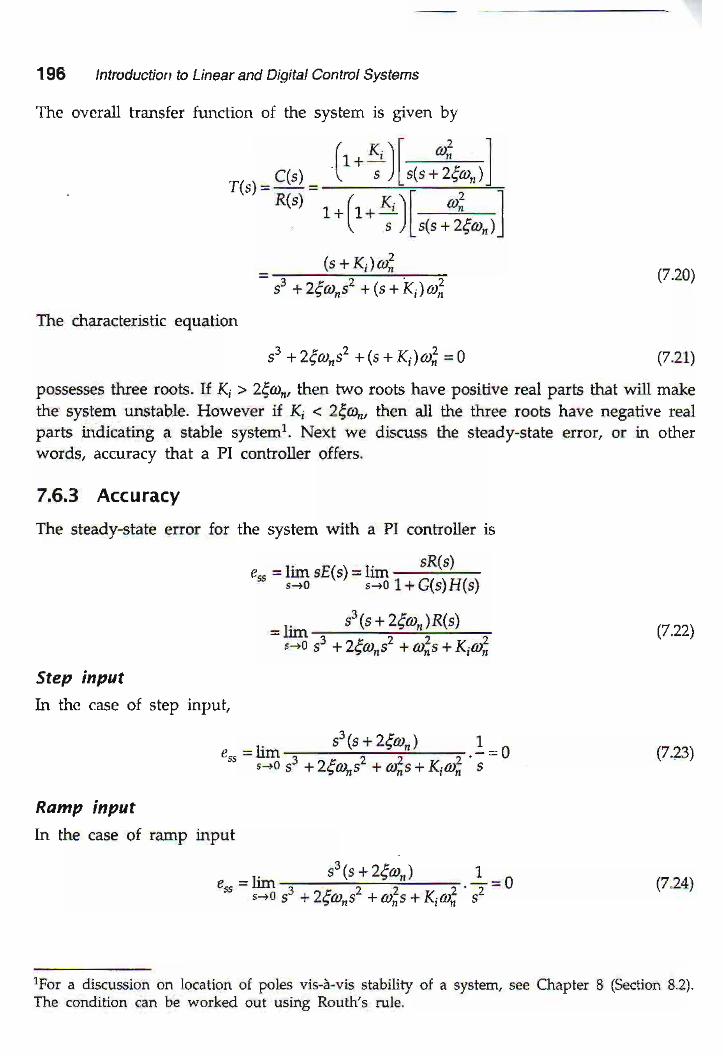
7.6.3 Accuracy

The steady-state error for the system with a PI controller is

sR(s)sss = rrm sE(s, = llrn:--:=#

s+u I + (,(srt,(s)

.. s3(s + 2{ar- )R(s)T-o s3 a l(6,s2 + aj,s + Kiafi

Step inputIn the case of siep input,

€"s

Ramp inputkr the case of ramp input

=lim s3 (s + 2lan1116 s3 + zlat s2 + fi,s + Kaafi,

' 1^

5

1^

Q.n\

v.n)

(7.24)=limT-i6 53 s 2.E6ne2 + afis + x,r,]

' s2

'

rFor a discussion on location of poles vis-i-vis stability oI a system, see Chapter 8 (Seciion g.2).The condition can be worked out usine Routh's rule.

/

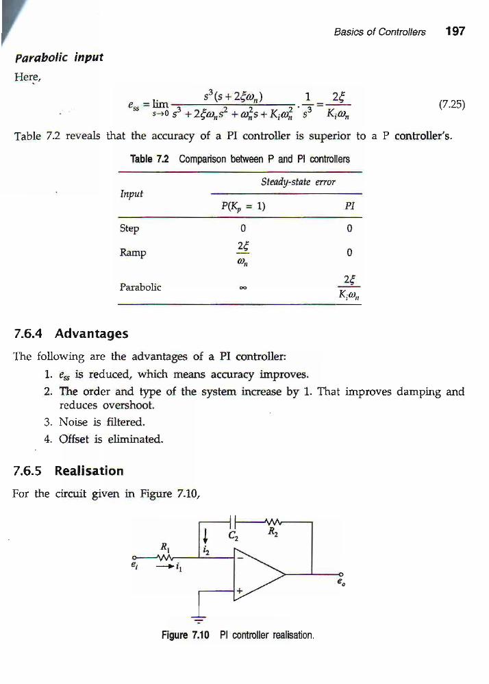
Parabotic input

Basic$ at Controlters 197

(7.25)

a P controller's.

Herg,

"., = t:a--r--!-!J4)- -

" ='€

s ao s" + 2E@^e + aj,s + K;afi, ' s3 Kian

Table 7.2 reveals that the acoracy of a PI conttoller is suPetior to

Table 7.2 Comparison bdrYeen P and Pl confiollers

Steady-state enorhtput

Ramp

ParabolicK;@o

7.6.4 Advantages

The following are the advantages of a PI controller:

1. e$ is reduced, which means accuracy imProves.

2. The order and t)?e of the system increase by 1. That imProves damping andreduces overshoot'

3. Noise is filtered.

4. Offset is eliminated-

7.6.5 Realisation

For the circuit given in Figure 7-10,

PI

0

0

0

,"

Figurc 7.10 Pl mniroller realisaton.

198 lntrcduction to Linear and Digital Control Systems

€ i r ,

The Laplace

', = [ I lrlo,, an, = uf J ;,, 1 ar * fr ",transforn of Eq. (7.26) yields

E"G) & 1Ei(s) Rr RrCz,

Ki=Kr*7

7,7 PROPORTIONAL PLUS DERIVATIVE (PD) CONTROLLERIn a PD conholler,

Its Laplace transform produces

,1"t t\a(t) = KDe(t) + K,t ::Y!

at

A(s) " ..t(s)

r tKr=1.

7.7.1 Control ActionU the error signal is a unit step, thm

a(t) = K"u(t\ + Kd ff

= X, * X odln

Flgure 7.11 Ac rating signat of pD contrcller for ramp error signal.

(7.26)

Q.2n

(7.281

(7.2e)

(7.30)

whirh indicaies that the actuating signal is an impulse. However, if the error signal isa rarnp, it is easy to see that the actuating signal is also a ramp lsee figure Z.ifj. -

Basics ol Conttolleg 199

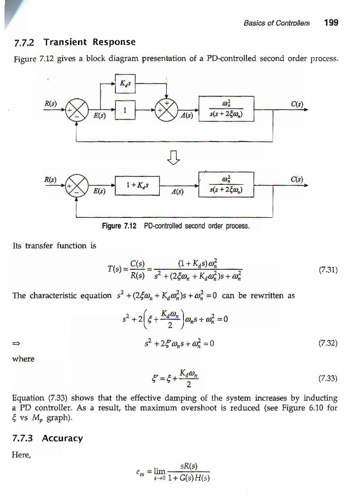
7.7.2 Transient Response

Fiatrre 7 -12 gives a block diagram Presentation of a PD-controlled second order process'

Its harsfer function is

ar<\ lI+ K,s)a;- '-' R(s) s' + (2ltt;, + Kda;)s + tt+,

(7.31)

v.32)

where

The charactedstic equation s2 + (29a,+ Kdz*)s + d = 0 can be rewritten as

,, *z(e *ff),"F+0*=o

s2 + z( ans + a|, =0

, - o -Ko'n

Equation (7.33) shows that the effective darnping of the system increases by indu:qtg

"=pO .o.titoU"r. As a result, the maxirnum

-overshoot is reduced (see Figure 5'10 for

( vs M, gapF.).

7.7.3 Accuracy

Here, .,,=$*#h

sG + 2ea)

PD-controlled second order process.

200 lntrcduction to Lineat and Digital Contot Systems

,. sz (s +zta-l= lun ; ' i' =s+o s' + (2lon + Kd(4)s + ot

(7.u)

(7.36)

vsn

(7.38)

e* =lim . sz G +2€a') -

" :-o s2 + (z(a, + Koal)s + ofi

Pdrabolic inputIn the case of pambolic input

s-\s + zgan) I! . . _ : l l l . . i - - - - _ l l l l - l l l l l ! i l l l l l l l ! i - . - = E-"' s-o s' + (z€a, + Kd(4)s + at sr

Step inputIn the case of step inpui,

Ramp inputIn the case of ramp input,

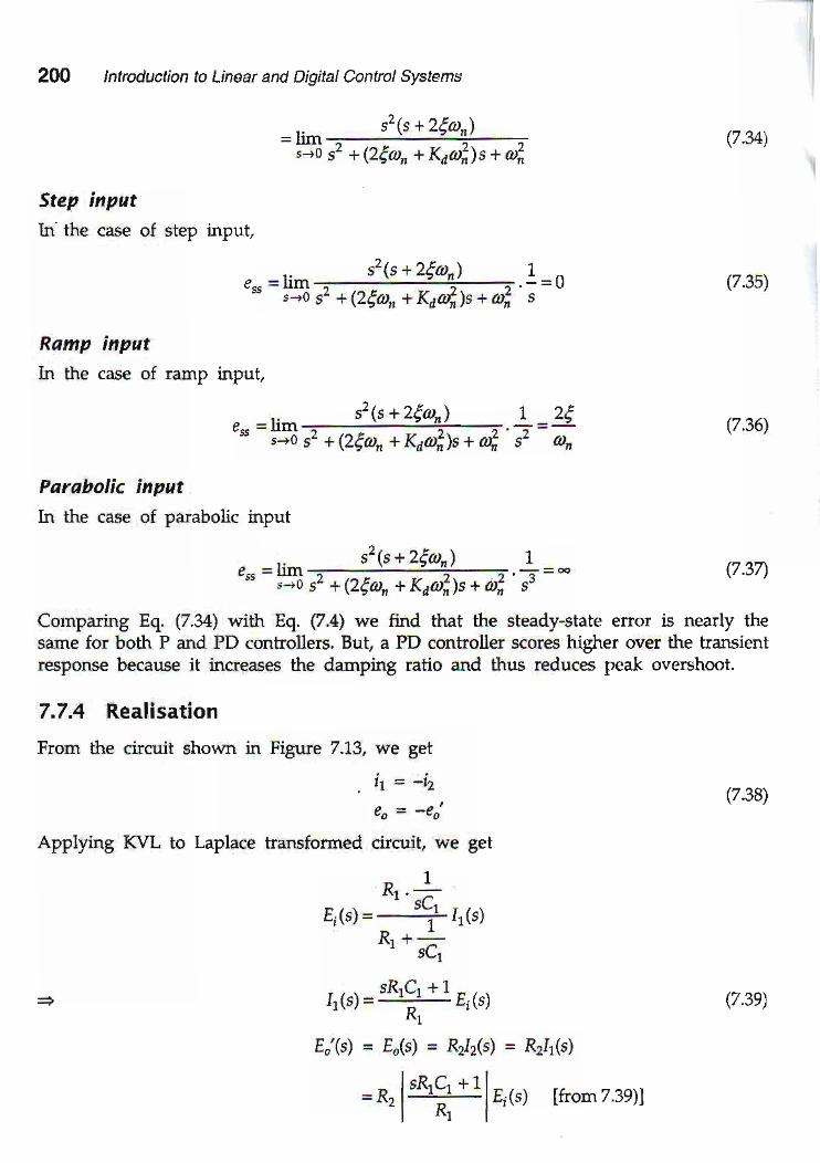
7.7.4 Realisation

From the chcuit shown in

Applyng KVL to Laplace

1_'I = u (7.35)

1 tF

s- @"

Complnlg Eq. (7.34) -with Eq._ (7.4) we find that the steady-state error is nearly thesame for both P and PD conhollers. But, a pD controller scores higlrer over the tansientresponse because it increases the damping ratio and thus reduci peal overshoot.

Figure 7.13, we gei

i=- ize" = -e;

transformed cfucuit, we get

&.1Ei(s, = ----i 11(s)

R, +-' sCr

, . . sR,C, +1- . .11(s)=-- t ' (s )

r"'G) = E,G) = R:rzG) = Rzrr(s)

- IsR'G +rl-. .=n' l=-lEts)

[from73e)l

(7.39\

F

EG)

Basi6 of Contrclters 201

(7.40)

(7.41\

Thus,

7.8 PROPORTIONAL PLUS INTECML PLUS DERIVATIVE (PID)CONTROLLER

As the name suggests, in a PID conholler the actuating signal has the following form:

a(t)= Kre(t\ + K, Iett) dt + x1ff (7.4)

The block diagram of the PID controller acfion is shown in Figure 7.14.

Figule 7.14 PID ctntrol aclion'

Without detailed analysis, we may say based on superposition of enors, tlnt sincethe PD conhol improves the transient Part and the PI control improves the steady-statepajt, a combination of PI and PD imProves the overall control

+h

Flgure 7,13 PD mntroller circuit.

202 Introduction to Linear and DigitalControl Systems

The op-amp realisation of PID controller is shown in Figure 7.15.

Table 7.3 presents a sunrnary of salient features of three basic modes of control to helpselect a controller for a particular process.

Table 7.3 Selecdon ot control ac{ion

Figurc 7.15 PID controller circuit.

Proportional action is chosen if Integral iction is choxn if Deriaatioe actiofl is chosen if

o Load changes are small.o Offset can be toleiated.o Error signal, which is

small, needs amplification.

Offset is not permitted-High degree of accuracy

o Transient lesponse param-etels such as rise time,maximum overshoot, etc.are to be improved upon.

o Plant load changes haveto be tracked by the con-tloller.

aD

7.9 RATE FEEDEACK CONTROLLER

Also called derioatiae feedback controller ar.d. output derioatioe controller, tf\is controllerincorporates derivative action in the feedback path as shown in Figure 7.16.

a( t )=e( t ) -KDdc(t)dt

Figule 7.16 Rate feedback control aclion.

Here,

(7.43)

7AG)=EG)-Kosc(s)

- --,r'o forward Path gain isl n L D " _ -

cG)=!11=s(s + 260")E(s) . . "Kod-

s(s + 2€a^)

== 'ts'+(2(ro,+Keai)s

The overall transfer function is

cG) - G(s)R(5) 1+ GG)

,t*

Basics ol con]/liollers 203

(7 M\

(7.45)

(7.46)

(7.47\

(7.48)

=- d . "s '+(2€a,+KDa;)s+at '

The characteristic equation is

s2 + (2(ro, + Keohs + tfi =g

, -2€a, + Koa*,' 2a^

- o -Kr 'n2

It is clear from Eq. (7.48) that the damPint rafio is increased' As a result (a) the mari-

mum overshoot is decreased, and (b) the nse-rime ts mcreaseo'--'l No-, let us ch€ck the effect on the steady-state ellor'

, =ri, ' '. sR(J)- 's ;n l rc( tH(t

- l, sts-'z + (264r" + Kpg;)slR(:)s 'o st + 121a, + Krai\s ' t'si'

_rn t^G+2€o,+Kp(!:)R(s\_ \7.4sl;-a 3z - 12(a^ L KDD;)S + a;

Step inputIn the case of steP inPut,

" = i^ ?ls- (2€a, - K=pot)l ^ .! =o {7.s0)=' i'jd s'] - (2€d" - KD(4\s+ a; s

204 lntroduction to Linear and DigitalContol Systems

Ramp input

s2ls +(21a)r+KDo?)l 7Here, e-- = lim"

-

"-ri r: + (2(a, - grrz 1t - S "2

2[a, + Krafi=---E-

(7.s1)

Parabolic input

In the case of parabolic input

o _ 1i- .s21s-+-(2€ot:_.+ K_p(4)l _ . L _ _ (7.s2)-*

;; r, + 12{t .r, - K nal,l s + d}, ' s3

A comparison between the PD controller and rate feedback controller, both of whichemploy derivative action, will be of interest here.

7.9.I Comparison between PD and Rate Feedback Controllers

1. The damping ratio increases in both the cases. As a consequence, peak overshootand settling time decrease while rise time increases in both the cases.

2. The PD controller introduces an additional zero at s = -I/Ka trt the closed-looptrarsfer ftrnction while the rate feedback controller does not. We have seen inSection 6.7.2 that the addition oI a zero reduces rise time but increases the peakovershoot. So, even if Ka = Ko, the responses will not be the same because of thiszero factor.

3. The type of the system does not change in both the cases which implies that thepattem of the steady-state error will remain the same for both the cases. However,by comparing Eq. (7.36) with Eq. (7.51) we find that the lamp input elror is higherfor the rate feedback controller.

Next, we define two importart parameters, namely integral square error (ISE) arrdintegral ibsolute error (IAE).

7.IO INTEGRAL SQUARE ERROR (ISE)

Unlike the steady-state error, the inte$al square enor is a measure of the system errortfuough the entire time, i.e. from f = 0 to f = -. It is defined as

2t , .an

$E=l* e2(t)dt

where e(f) = error siSnal.

(7.s3)

For examPle,

Therefore,, ) l t 1 , -

rse = J- f4- sur'1 l\a^.lr

- ( )t + 0] dt whete o = co{' €

r f r,,r l (7.5s)= 2'J_filE-")

:ffjtffi g"t3,"ii'fii,?Jft ihe IsE is dependent on two ractors' namelv damping

Basics of Controllers

for the unit step inPut to a second order system

"-ia t f' t--

.o = -ft t' | (,",11 - ( )r - cos-' 4l

\ i r - 9

205

(7.s4t

7,11 INTEGRAL ABSOLUTE ERROR (IAE)

The integral absolute error is a measure of average erlor over

and is defined . r

teE = Jn le(t) ldt

EXAI/IPLE 7.1 (a) A unity feedback position control system has a-forward path transfer

tunction G(s) = K/s. Fot o^t "d

;i;;t compute the value of K that minimises lSE'

@) The transfer ftnction of a system is 1/(1 + sT) The input to the system is 'u(t)'

f}r" ,]"ip"i-*o"fa track the system Find the value of the ste.ady'state erroi'

Solulion: (a) Given, G(s) = K/s' H(s) = \'

' ,r" =99)' ' - ' R(s)

= G(s)1 + G(s)

Ks+K

KfC(s) =----::- L.

5 (s t ^ , L

L1

a certain time Period, T,

\7 -56)

R(,) = 1ls l

The inve$e LaPlace

s s+K

transform Yieldsc( t )=1-

e(t) = e-Kt

1.zOG lntroduclon to Linear and Digital Controt Systens

Therefore,

lSE= | e ' " 'd tJ o

o-2Kt l'

2i( [

1=2K

This result indicates that ISE -t 0 as K r *.

O) Given,

G(s) = 1' 1+ sT

and since the output would track the system, H(s) = 1.41"o,

r ( t ) = tu( t ) = t fo r t>0

+ RG)=+Therefore,

,. sR(s)-'s ;:d 1+ c(s)H(s)

,. -. ls ( r+s l ) . ,

= l l l t l -s io 2+ sT

Altemativelt we can find the same result from the following study in the t-space. Here,the closed-loop transfer function is given by

C(s) _ G(s)R(s) 1 + GG)

1= 2+tT

Therefore,1/T

L(s.) = ---7-----;T

s- ts+* |\T /

/ 1 D L- - - t - -7 - - - - - - ; -

\5dy ,

Basics of Controllers 207

ihen,

,l 1 1l 'r-l

=-i7-lTl =- 4"-71"=o l'*iJ l.=.

1l r=71,,=-z=i

1TTC(s)='--=--+--7--;

Z , : J , l ^ , - |

\ r . /

, - - 2 1

c l =- - -+-e ''244

e." = rim h(r) - c(f)l

f . - l z r \ l=L^ll+' l1-"-i l lr-*12 a( l l

_, , c(s)' R(s)

18s2 + 2.6s

18'-?

* L6t

r )la=,,c(,)1,=o=+l+ll =i

I J - ; J I\ r . , l !=o

,=ft1*rt',1,="=l!,

.=[,.i).orl,__,

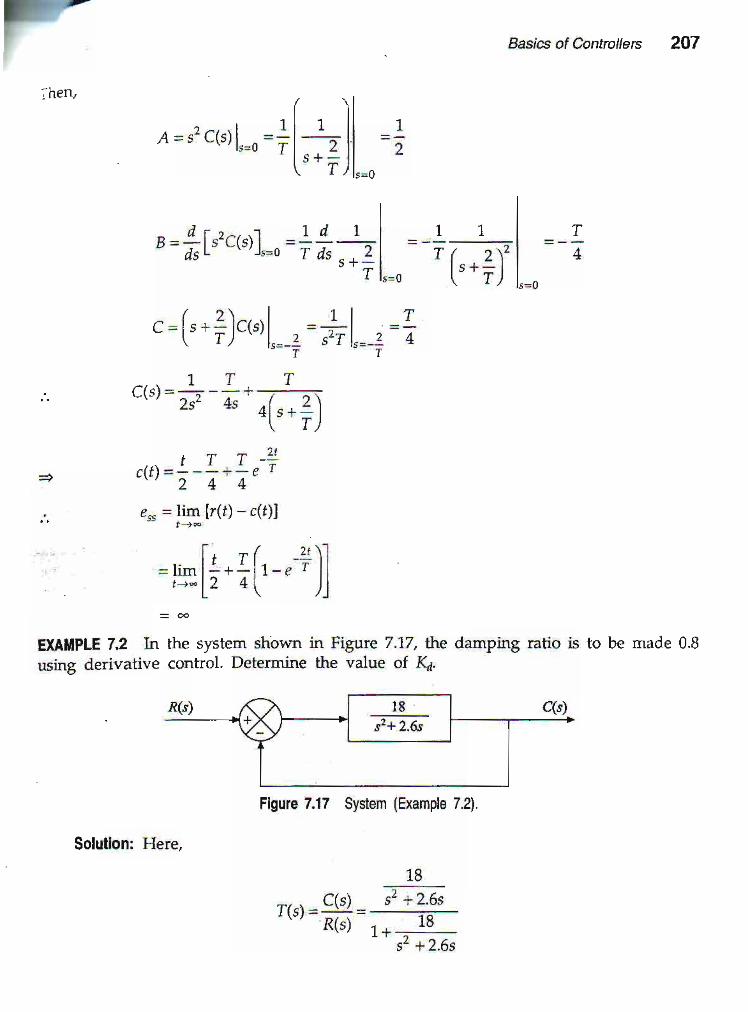
EXAI|PLE 7.2 In the system shown in Figore 7.17, the damping latio is to be made 0'8

using derivative control. Determine the value of K4'

Figure 7.17 Syslem (Exampl€ 7.2).

Solution: Here,

or

208 lntroduction to Linear and Digital Contrcl Systems

18sz +2.6s +18

Therefore, the characte stic equation is

By comparisory

s2 +2.5s+18=0=s2 +2(rons + of i

4=Ba, = 4'243 rad/ s

2€t'+ = z'0- 2 .O4=

- - =0.3' (2)(4243)

derivative control, 6'has to be 0.8. So,

- - Kaa-€ =E+_z_

= Ko=V-gL@n

= (0.8 - 0.3) 2 =0.24' ' 4.243

EXAi|PLE 7,3 hr the system shown in Figre 7.18, determine the derivative feedbackconstant I(o which will increase the damping factor of the system to 0.6. What is thesteady state eflor to unit ramp input with this setting of the derivative feedbackconstant?

or

Now, with

Solutlon: Given,

transfer function of the

Figure 7.18 System (Example 7.3).

1Gr G) = -:- and H1 (s) = sKo

irurer feedback loop is

G(s) =Gr(s)

1+qG)H1G)

1

tne

s(s+2)+sK,

Basics of Controllers 209

.nd the overall transfer

The characteristicequation is,

By comParisorL

or

or

Therefore,

EXAI'PtE7.4 Figure

function is

- . . Or(s) K,GG)I l s )= -= -" On(s) 1+K^G(s)

K^s(s+2)+sKo+Ka

10s2 +(2+4)s+10

s2+(2+IQs+10=0

= s2 +2(atos + afi

o ;=]u

a" = 3.762 nd/s2ea,=2+19

&=21a^-z= 2(0.61(3.762) - z= 1.8

.. sO" (s)-""

;ii 1+ KAc(s)

1- ' - 2

: lim -------------!-; -d , . 10'-?.rr* lst

=lim s+3.8s-ro s' + 3.8s + 10

= 0.38

the block diagram of a position contlol system.7.19 shows

AEplifie!

Flgure 7.19 Positionctnlrolsystem (Example 7.4).

21O Intrcduction to Linear and Digital Control Systems

(a) In the absence of the derivative feedback, i e', Kl = 0, determine the damPing ratio

of the system for amplifier gain KA = 5'

(b) Find the suitable values of parameters Ka and K1 so that the damping ratio of-the*'

;yrt"^ is increased to 0.7 without affecting the steady-state error as obtained in

part (a).

Solulion: (a) Here,

5

rG)=ffi=s(0.5s + 1)

r -u ---i-- s(0.5s + 1)

Therefore, the characteristic

*

By comparison,,4=ro(4 = 3.'162 lad/s

zEa" = Z

q=-f-=s.s153.1,62

(b) Steady-state error (for a ramp input) for palt (a)

'" =telS*-_ .-o 1+ do;*1)

s2 + 2s+ 10

equation is

+2s+10=0

= sz + 2(ans + afi,

0.5s + 1=lim

,+0 s(U.5s + I) + )

- n t

the inner loop rs

1s(0.5s + 1)

s(0.5s + 1)

1

Now, the trarufer function for

qG)=

s(0.5s+1)+sKi

Basi6 ot contoltels 211

ro, the overall transfer function is

rto=91')=, Kt9'l'1,-'

R(s) 1+ KaQ(s)

KAs(0.5s+1)+sK1=;----E^

-- s(0.5s + 1)+ s(1

KA

05s2 +(K1 +1)s+KA

Ka /0.5-- -'-------7;L'-"

2 Kr+r . l (A

The characteristic equation is

. K+1 K, ^5 _ T - : = - j - - - = = \ ,

u.5 u.J

= s2 +2(ais + aiz

By comPariso&

,f =#' tx;or a; =h5

ztu;=T

or P=Kt+ l ' L

' - 0.5 'zt ;

- t v L 1 \ I : =_..., , 1'{r(e

= 0.7 (grven)

0.7J0.5

(0

Now.1,

sx- - te" = lin]

s-eo r r\Alf---.------::.---:-

s (0.5s + 1) + s&

212 lnboduction to Linear and Digitat Control Systems

=lim 0.5s+1+Kr

Dividing Eq. (i)

Kr +1

by Eq. (ii), we get

sro s(0.5s + 1+ Kl) + K,{

1+KKA

=02 ldetermined for part (a)] (ii)K^

n7JK'=d(ot

Kt = 24.5

l(r = U.ZK,q - 1 [From Eq. (ii)]- l o

1. Choose the correct answer:(a) Excellent transient and steady state resporue is provided by

(i) a proportional action system(ii) a proportional + differential action system(iii) a proportional + integral + differential action system(iv) none of the above

(b) Derivative controllers are nevel used alone because of(i) their large input impedance

(ii) they amplify noise signal and cause saturation of the actuator(iii) they worsen the frarLsient response of the system(iv) none of the above

(c) The measure of average error(i) integal absolute error

(ii) inte$al square enor(iii) steady-state error(iv) none of these

(d) Igtcl of the following control actions is to be employed for eliminating theoffset?(i) Proportional control

(ii) Proportional plus derivative conhol(iii) Propodional plus integral control(iv) None of these

over a specified time period is called