3.1 tactical 0-2 hour convective weather …classification module. this same high resolution echo...
TRANSCRIPT

1
TACTICAL 0-2 HOUR CONVECTIVE WEATHER FORECASTS FOR FAA†
M.M. Wolfson*, B.E. Forman, K.T. Calden, W.J. Dupree, R.J. Johnson Jr., R.A. Boldi, C.A. Wilson, P.E. Bieringer, E.B. Mann, and J.P. Morgan
MIT Lincoln Laboratory, Lexington, Massachusetts
CONTENTS (PAGE #) 1. INTRODUCTION 1 2. DEVELOPMENT OF THE CWF
TECHNOLOGY 1 3. DESCRIPTION OF THE TACTICAL 0-2 HR
CWF ALGORITHM 5 3.1 Overview 5 3.2 Tracking the Radar Data 7 3.3 Mosaicing Multiple Radars Together 9 3.4 CWF Processing 10 3.4.1 Weather Classification 10 3.4.2 MultiScale Tracking 13 3.4.3 Growth and Decay Trending 15 3.4.4 Initial and Final Forecast Combination 15 3.5 CWF Scoring 18 3.6 CWF Display 23 4. STATUS OF CWF FOR ITWS AND CIWS 27 5. FUTURE WORK 28 5.1 Including Convective Initiation 28 5.2 Coupling Forecasts to ATM Automation Tools 30 5.2.1 Forecast Error Model 30 5.2.2 Echo Tops Forecasts 32 5.3 Coupling Forecasts with NWP Models 33 6. SUMMARY 34 7. REFERENCES 34
1. INTRODUCTION
Major airlines and FAA Traffic Flow Managers
alike would prefer to plan their flight routes around convective weather and thereby avoid the tactical maneuvering that results when unforecasted thunderstorms occur. Strategic planning takes place daily and 2-6 hr forecasts are utilized, but
†This work was sponsored by the Federal Aviation Administration under Air Force Contract No. F19628-00-C-0002. Opinions, interpretations, conclusions, and recommendations are those of the authors and are not necessarily endorsed by the U.S. Government. *Corresponding author address: Dr. Marilyn M. Wolfson, MIT Lincoln Laboratory, 244 Wood Street, Lexington, MA 02420-9108; e-mail: [email protected]
these early plans remain unaltered in only the most predictable of convective weather scenarios. More typically, the ATC System Command Center and the Air Route Traffic Control Centers together with airline dispatchers will help flights to utilize jet routes that remain available within regions of convection, or facilitate major reroutes around convection, according to the available “playbook” routes. For this tactical routing in the presence of convective weather to work, both a precise and timely shared picture of current weather is required as well as an accurate, reliable short term (0-2 hr) forecast. This is crucial to containing the system-wide and airport-specific delays that are so prevalent in the summer months (Figure 1), especially as traffic demands approach full capacity at the pacing airports.
This paper describes the Tactical 0-2 hr
Convective Weather Forecast (CWF) algorithm developed by the MIT Lincoln Laboratory for the FAA, principally sponsored by the Aviation Weather Research Program (AWRP). This CWF technology is currently being utilized in both the Integrated Terminal Weather System (ITWS; Wolfson et al., 2004) and the Corridor Integrated Weather System (CIWS; Evans et al., 2004) proof-of-concept demonstrations. Some of this technology is also being utilized in the National Convective Weather Forecast from the Aviation Weather Center (Megenhardt, 2004), the NCAR Autonowcaster (Saxen et al., 2004), and in various private-vendor forecast systems. 2. DEVELOPMENT OF THE CWF TECHNOLOGY
Development of the Tactical 0-2 hr Convective
Weather Forecast began in 1996 with the formation of the FAA AWRP Convective Weather Product Development Team. A timeline of key demonstration and technology transfer milestones achieved as the CWF technology was being developed is shown in Figure 2.
Proceedings of the 11th Conference on Aviation, Range and Aerospace Meteorology, Hyannis, MA 2004
3.1

2
OPSNET Weather Delays
05
1015202530354045
Jan
Feb Mar AprMay Ju
n Jul
Aug Sep OctNov Dec
Month
Thou
sand
s of
Del
ays
20042003200220012000199919981997
Figure 1. Weather-related delays (> 15 min) as recorded in OPSNET. The summer months consistently show the largest delays, illustrating the effects of convective weather on the NAS. Figure 2. Timeline showing Demonstration Milestones (above time line) and Technology Transfer Milestones (below time line) during the development of the Tactical Convective Weather Forecast algorithm.
1998: 1-hr Forecast in ITWS
Dallas Orlando New York Memphis
2004: CWF, VIL and new Tracker
technology transfer to ITWS production
contractor
2002: 2-hr Forecast in CIWS
1996 1997 1998 1999 2000 2001 2002 2003 2004
Demonstration Milestones
Technology Transfer
Milestones
2002: NEXRAD ORPG Hi-res VIL
New Old
New Old
Licensed to 6 companies
1999: G&D Tracker Patent
2003: NEXRAD ORPG Hi-res Echo Tops
2003: Winter CWF Forecast1998: 1-hr Forecast in ITWS
Dallas Orlando New York Memphis
2004: CWF, VIL and new Tracker
technology transfer to ITWS production
contractor
2002: 2-hr Forecast in CIWS
1996 1997 1998 1999 2000 2001 2002 2003 2004
Demonstration Milestones
Technology Transfer
Milestones
2002: NEXRAD ORPG Hi-res VIL
New OldNew Old
New OldNew Old
Licensed to 6 companies
1999: G&D Tracker Patent
2003: NEXRAD ORPG Hi-res Echo Tops
2003: Winter CWF Forecast

3
The development of the Growth and Decay
Tracker technology described in Wolfson et al. (1999) provided a breakthrough that allowed operational forecasts of up to 1-hr to be fielded. The Terminal Convective Weather Forecast was demonstrated in the ITWS testbeds operated by MIT Lincoln Laboratory, first in Dallas (1998), then in Orlando and New York (1999), and finally in Memphis (2000) in an official “Demonstration/Validation.” The product concept involved an animated loop showing 30 min of past weather and 60 min of forecast weather, in 10 min increments (10 images per loop).
This initial work also pioneered the use of high
resolution Vertically Integrated Liquid water (or VIL) derived from NEXRAD radar data as a better representation of the convective hazard to aviation than the Composite Reflectivity used in ITWS (Crowe and Miller, 1999) or the Base Reflectivity used in WARP (Robinson et al., 2002). Smalley and Bennett (2002) worked to insert the new high resolution VIL used in the CWF demonstrations into the NEXRAD Open Radar Products Generator (ORPG), thus making it available as a Level III NEXRAD product for eventual use in FAA weather systems.
The Dem/Val user evaluation by the FAA
Technical Center staff indicated that the CWF “was viewed favorably by almost all participants in terms of utility, task benefit, benefit beyond ITWS, and interface characteristics. The overall impression of the product was positive.” They analyzed the TRACON and TMU task benefits to understand specifically how the product helped the traffic managers (FAA DOT, 2001).
A cost/benefit analysis was performed during
the Memphis 2000 Dem/Val by MCR Federal, Inc. (2001), who also utilized the task analysis approach and structured interviews to estimate dollar benefits of the improved performance of traffic management tasks. They estimated benefits in New York, Dallas, and Orlando/Jacksonville, and used these numbers, in conjunction with thunderstorm climatology, to estimate the national benefit. MCR Federal found that inclusion of CWF in ITWS would provide annual benefits that were very high.
The Lincoln Laboratory Dem/Val CWF
algorithm performance evaluation (Theriault et al., 2000, 2001) showed many cases of excellent
performance. However, critical analysis of all the data revealed several cases where performance was sub-optimal. Research identified the main causes of the incorrect forecasts were a) the use of a single track vector quality control constraint (each “local” vector’s direction had to be within ± 70 degrees of a single “global” vector’s direction or it would be eliminated), b) tracking artifacts arising from excessive smoothing of small cells in the precipitation images before they were tracked, and c) the lack of explicit growth and decay in the forecast.
These problems were addressed with three
key enhancements in preparing the CWF algorithm for eventual technology transfer, which are discussed in detail in Section 3 of this paper: a) a new “local-global” quality control constraint was developed for the ITWS Tracker (Section 3.2), b) CWF Weather Classification and MultiScale Tracking modules, which permit tracking of small storms and line storms equally well, were added (Sections 3.4.1 and 3.4.2), and c) a Growth & Decay Trending module, which provides growth and decay of existing storms, was developed for the CWF (Section 3.4.3).
The Corridor Integrated Weather System
(CIWS) concept exploration demonstration was fielded in 2000, when it became clear that “terminal” operations in the northeast actually stretched over several states and covered both enroute and terminal airspace in a busy “corridor” configuration (Figure 3). While CIWS debuted with a version of the 1-hr forecast used for ITWS, it also became clear that traffic managers in the Corridor required a longer lead time forecast because of their large geographical area of concern.
The CWF enhancements stemming from the
Memphis 2000 Dem/Val provided a sufficient increase in forecast accuracy to enable the extension of forecast lead time from 1 hour to 2 hours, thus making the forecast much more useful to enroute traffic managers and other users of CIWS. The 2-hr Forecast for CIWS was first demonstrated in August 2002. The product concept was much like ITWS with an animated loop, but the loop interval stretched from 60 min in the past to 120 min in the future, in 15 min increments (13 images per loop). A CIWS benefits assessment conducted in 2003 (Robinson et al., 2004) identified the 2-hr Forecast and the Echo

4
Tops product as the two most heavily used products by the users (Figure 4). The CWF algorithm now makes use of the Echo Tops information internally for its Weather Classification module. This same high resolution
Echo Tops product has been coded for the NEXRAD ORPG by Smalley and Bennett (2002), and is now available as a Level III NEXRAD product.
2003 CIWS Products Usage
2-hrForecast
EchoTops
NEXRADPrecip
G&DTrends
495
363 350
262
217
44 39 34 21 18
0
100
200
300
400
500
600
StormMotion
Lightning ASRPrecip
ForecastAccuracy
Verif.Contours
Satellite
Num
ber o
f Obs
erve
d Pr
oduc
t App
licat
ions
2-hr Forecast
2003 CIWS Products Usage
2-hrForecast
EchoTops
NEXRADPrecip
G&DTrends
495
363 350
262
217
44 39 34 21 18
0
100
200
300
400
500
600
StormMotion
Lightning ASRPrecip
ForecastAccuracy
Verif.Contours
Satellite
Num
ber o
f Obs
erve
d Pr
oduc
t App
licat
ions
2-hr Forecast
Figure 3. 24-hr traffic counts over the continental United Stated on a clear weather day (12-13 September 2002), showing the high traffic density in the Northeast Corridor, where several major terminals are located. The strong coupling between terminal and enroute delay in this area motivated the 2-hr forecast horizon for CIWS, to help improve management of the congested enroute traffic.
Figure 4. Chart from Robinson et al. (2004) showing the frequency of use of each of the CIWS products during the intense observation periods when MIT LL staff were onsite at several of the enroute centers in the CIWS domain and at the ATC System Command Center.

5
The CWF algorithm was further enhanced in 2003, in response to the need for high quality year-round forecasts expressed by the New York ITWS and CIWS user community. The CWF algorithmic logic that suppressed stratiform rain signatures (because there was no threat of convective weather in those locations) was not appropriate in the winter, when the majority of weather fell into the stratiform or non-convective category. The forecast of a moderate to heavy stratiform rain or snow event would show less and less precipitation with time, eventually emptying the screen of all indication of forecast precipitation. With the release of the 2004 CWF algorithm, the forecast is purely deterministic, depicting at every forecast time horizon an estimate of what the radar will show in the future. A new user-selectable Winter color scale to enable depiction of significant structure within weak radar returns (i.e., within the level 1 precipitation band) was also added. This will be particularly important in the northern part of the CIWS domain, including the major terminals such as Chicago, New York, Detroit, Cleveland, Boston, and Toronto.
The final milestone shown in the Figure 2
timeline is the 2004 technology transfer of the 1-hr Terminal Convective Weather Forecast to the ITWS production contractor. With this milestone met and the contractor development of TCWF underway, we can look forward to operational deployment of this new capability in FY06. The following chapter describes in some detail the major elements of the FAA Convective Weather Forecast algorithm that was transferred to ITWS in March, 2004. This same CWF technology is used in CIWS, and the differences are pointed out specifically in Section 4 where the status of the CWF algorithm for both ITWS and CIWS is discussed. Section 5 points out some of the research efforts underway to increase the operational utility of the Tactical 0-2 hr Convective Weather Forecast. 3. DESCRIPTION OF THE TACTICAL 0-2 HR CWF ALGORITHM
3.1 Overview
The Tactical 0-2 hr Convective Weather
Forecast (CWF) algorithm is fundamentally a multi-scale storm tracking algorithm that internally determines the type and strength of existing storms, their motion and growth/decay trends, and forecasts their evolution based on models
developed from thunderstorm case studies. For example, thunderstorms can be broadly categorized into “airmass” and “line” storms (Figure 5). Airmass or single cell storms are small scale, seemingly random, fairly disorganized convective elements. Line storms or multicell storms are a collection of cells much like airmass cells, but they are maintained in an organized linear pattern or “envelope by their forcing mechanisms. These more organized storms tend to persist longer and evolve less rapidly than the airmass cells. In the CWF algorithm, all storms are tracked, classified according to weather type, and measured growth/decay trends are fed into models that determine the eventual evolution of the storms. The storms are advected to their predicted location and altered in size and strength to produce the forecast.
A schematic overview of the CWF algorithm
processing is presented in Figure 6. The diagram is color-coded according to algorithm timing, where it can bee seen that the CWF algorithm processing takes place in two main parts: one “per radar” part that triggers upon receipt of each radar’s complete scan of data, and the other “clock-driven” part based on the entire grid, once the mosaicing has taken place. The MultiScale storm tracking also takes place in two parts.
Beginning before Box 1 in Figure 6 at the data
ingest, polar VIL data comes into the processing stream from a set of NEXRAD and/or TDWR radars. In the case of NEXRAD, polar VIL could be derived from Level II base data or read directly from the new Level III High Resolution VIL product, which has already passed through some data quality assurance steps prior to VIL processing in the NEXRAD Open Radar Product Generator. In the case of TDWR, an algorithm similar to that used in NEXRAD is used to generate polar VIL from the radial TDWR reflectivity data.
The polar VIL data is gridded and sent to the
numbered boxes, which are described briefly in Table 1. The incorporation of VIL from the NEXRAD/TDWR radars as part of the CWF permits the replacement of maximum composite reflectivity with VIL as the new Long Range Precipitation product for ITWS. The inclusion of Mosaic Processing for multiple NEXRAD/TDWR radars (Box 3) represents another large enhancement for ITWS.

6
Figure 5. Models of two major storm types: airmass storms and line storms. Idealized vertical cross sections of the storms, their plan-view appearance in radar data, and a heuristic depiction of their life cycle are shown.
0 5 10 15 20 25 30 35
12
9
6
3Hei
ght (
km)
Time (min)
0 10 20 km"Dissipating""Mature""Cumulus"
14
12
10
8
6
4
20 –18 –16 –14 –12 –10 –8 –6 –4 –2 0 2 4 6
Distance Ahead of Outflow Boundary (km)
Storm Motion –40°C
–20°C
–0°C
SN
Hei
ght (
km)
Model of Storm Type Appearance inRadar Data Storm Life Cycle
Time
Wat
er C
onte
nt
Time
Wat
er C
onte
nt
0 2 4 6 8 hr
Multi-cell or “Line” Storms
Isolated or “Airmass” Storms
• Solar forcing• Short-lived, small scale• Largely disorganized
• Large scale forcing• Long-lived, large scale• Highly organized
0 2 4 6 8 hr
0 5 10 15 20 25 30 35
12
9
6
3Hei
ght (
km)
Time (min)
0 10 20 km"Dissipating""Mature""Cumulus"
0 5 10 15 20 25 30 35
12
9
6
3Hei
ght (
km)
Time (min)
0 10 20 km"Dissipating""Mature""Cumulus"
14
12
10
8
6
4
20 –18 –16 –14 –12 –10 –8 –6 –4 –2 0 2 4 6
Distance Ahead of Outflow Boundary (km)
Storm Motion –40°C
–20°C
–0°C
SN
Hei
ght (
km)
14
12
10
8
6
4
20 –18 –16 –14 –12 –10 –8 –6 –4 –2 0 2 4 6
Distance Ahead of Outflow Boundary (km)
Storm Motion –40°C
–20°C
–0°C
SN
Hei
ght (
km)
Model of Storm Type Appearance inRadar Data Storm Life Cycle
Time
Wat
er C
onte
nt
Time
Wat
er C
onte
nt
0 2 4 6 8 hr
Multi-cell or “Line” Storms
Isolated or “Airmass” Storms
• Solar forcing• Short-lived, small scale• Largely disorganized
• Large scale forcing• Long-lived, large scale• Highly organized
0 2 4 6 8 hr
Figure 6. Block diagram of the processing involved in the Tactical 0-2 hr Convective Weather Forecast algorithm. Processes in pink boxes update upon receipt of radar data (~3-6 min), the green box indicates receipt of RUC data (~1 hour), the blue process updates at a 2.5 min clock rate, and the gray processes update at a 5 min clock rate or upon receipt of forecast algorithm output.
1. Data Quality Editing
2. CWF Per Radar Processing
- Filter and Track
- Growth & Decay Trends
3. Mosaic Processing
4. CWF Full-Grid Processing
- Weather Classification
- MultiScale Tracking
- Initial and Final Forecast Combination
5. CWF Scoring
6. Display Product Server
7. CWF Display Processing
CWF Algorithm Processing
Radar Data Ingest
RUC Model
Data Ingest
Grids for display
Forecast Grids for display
Per radar ~ 3-6 min
2.5 min (clock)
5.0 min (clock)
RUC data ~ 1 hr
Timing Color Key
Per radar ~ 3-6 min
2.5 min (clock)
5.0 min (clock)
RUC data ~ 1 hr
Timing Color Key

7
The balance of the CWF Algorithm Processing
diagram shows inclusion of the Rapid Update Cycle (RUC) numerical model data at approximately 1-hr time intervals (green) into the 5-min CWF Processing (Box 4, shown in gray), the creation of forecasts and scoring information (Box 5), and the preparation of data for display (Boxes 6 and 7). These steps are described in more detail below.
3.2 Tracking the Radar Data
For purposes of obtaining magnitude and
direction of storm cell and storm envelope motion, a “cross-correlation tracking” method is employed. A full description of the cross-correlation tracker (hereafter denoted XCT) can be found in Chornoboy et al. (1994). This section describes the enhancement made to the ITWS XCT algorithm for use in CWF, introducing the local quality control constraint of the correlation track
Box Update Rate
Component Name Description
1 Per input radar
Data Quality Editing Removes small, thin, isolated non-meteorological regions (dubbed “lint”). This filtering is applied to both VIL and Echo Tops data.
2 Per input radar
CWF Per Radar VIL Processing - Filter and Track - G&D Trends
Part of the core CWF Processing. (a) Tracks storm motion using multiple instances of the modified ITWS cross-correlation tracker, each optimized to track features with different spatial and temporal scales. (b) Computes growth/decay trend images containing information about the evolution of storm elements.
3 2.5 min clock
Mosaic Processing
For each type of data generated by the Per Radar processes 1 and 2, an instance of the Mosaic Process reads all the input radar data and combines it into a single output stream. For all input except the vector lists, the Mosaic algorithm generates an output grid showing the union of all the input images using a set of region-specific rules to decide how to merge the overlap regions. For the vector lists, the Mosaic algorithm generates one master output list that is the union of all the input lists. Additionally, for both types of inputs, the data are advected to a common time prior to output. This process is referred to as “Time-aligning” the data.
4 5 min clock
CWF Processing
The bulk of the core CWF Processing. This algorithm: (a) classifies the type of Weather (WxType) at each pixel in the input image; (b) associates an appropriate scale motion vector with each pixel based on the WxType, creating the MultiScale vectors; (c) applies scoring functions based on models of thunderstorm evolution and measured growth/decay trends, VIL, and WxType, to transform the inputs into unadvected forecast images for each forecast time horizon; (d) advects the forecast images to their forecasted position using the MultiScale vectors, and (e) applies further corrections to the forecasts in their advected locations based on environmental stability.
5 Receipt of forecast output
CWF Scoring Computes the recent skill of the forecast system by comparing past forecasts with the current weather; also provides contours of the forecast images.
6 Receipt of forecast output
Display Product Server
An interface between the CWF system and the display system. This is where rescaling, clipping, and any other strictly display related preprocessing occurs.
7 Receipt of forecast for display
CWF Situation Display Processing
This algorithm merges the appropriate past weather images with the current weather and forecast images in preparation for display. It also stores the current weather at each update for future use in building the loop of past weather images.
Table 1. Major Processing Components of the CWF System

8
vectors. XCT is one of the core building blocks of CWF MultiScale tracking, which is discussed further in Section 3.4.2.
For ITWS currently, all local motion vectors
are constrained using a single, so-called “global” motion vector which is meant to capture the average motion across the entire image. Typically if a local vector is not within ± 70 degrees of the global vector, it will be flagged as invalid and later filled in by interpolation. The intent of the global constraint vector is to impose some degree of uniformity on the field of local motion vectors. Unfortunately the use of a single global vector to constrain all local motion vectors can be seriously flawed in some circumstances. This is particularly true in the case of a hurricane or any other circulation feature, where there can literally be a valid 360 degrees of motion within a single image (i.e., the set of motion vectors immediately around the eye of a hurricane).
In order to impose some uniformity on the
vector motion field without constraining the vectors in a way which prohibits accurate portrayal of the actual motion, for CWF we introduced the idea of a “local-global” constraint. Effectively, a “global” vector is computed within a relatively small sub-grid of the full motion grid. This “local-global” vector is generally constructed as a weighted
average of the raw motion vectors within the subgrid. The averaged vector is then used to constrain only that raw motion vector located at the center of the corresponding subgrid. Thus, each single local vector has its own associated constraining vector. Since there is considerable overlap in the subgrids when going from one analysis location to the next, local smoothness of the final vector field is enforced, and adjacent raw vectors will necessarily have roughly equivalent constraining vectors. But since the subgrids for two vectors which are "far apart" within the image will have no overlap, they are free to have very different constraining vectors.
The result of using the local-global method for tracking the Hurricane Claudette case is contrasted with the ITWS single-global method result in Figure 7. With local-global, the full 360 degree range of motion around the hurricane eye is now captured. Small subgrids of vectors on the south side of the eye tend to average out to an eastward constraining vector, while small subgrids to the east of the eye tend to average out to northward constraining vectors, etc. Again, local uniformity is enforced, but as one traverses large distances within the image (say from well south of the eye to well north of the eye) very different constraining vectors are obtained.
global motion local motionsglobal motion local motions
Figure 7. Motion vectors in Hurricane Claudette constrained with the new “Local-Global” setting for the ITWS cross-correlation tracker.

9
3.3 Mosaicing Multiple Radars Together Some parts of the convective weather forecast
system are run on data from individual radars, and others parts are run on data merged or mosaiced together from multiple radars into one image. This section describes the process used to merge data from individual radars into mosaiced images.
Currently four mosaic processes take place in
the CWF system to merge four different data types: Vertically Integrated Liquid water (VIL), Echo Tops, precipitation Growth and Decay Trends, and Storm Motion. The mosaics are triggered on a 2.5 min clock for display of products, and CWF makes use of every other set of mosaics in its five minute update rate. Even with a 2.5 min clock trigger, there will still be small differences between the radar data volume end times and the clock trigger times. To compensate for this, a time alignment step is executed in which the storm motion image derived from that radar’s VIL data is used to advect the radar data from its volume end time to the trigger time. If a data set is too old (e.g., > 15 min), it is dropped out of the mosaic. The motion-compensated data are then merged.
The logic to decide what value to put into the
mosaic output image in locations of overlapping coverage varies depending on the type of product
being mosaiced. Storm Motion vectors are simply interpolated into a mosaiced image. For the Echo Tops product, the maximum value is currently selected in places of overlap, although enhancements to this logic are planned. For the VIL product, the “maximum plausible” value is selected. The “maximum plausible” algorithm is biased towards using the maximum VIL value of a radar within a given range (nominally 230km) unless it is found to be “not plausible” given what is shown by the other radars at that location. If the highest value is not deemed plausible, it is not used in the mosaic. This reduces clutter and anomalous propagation (AP) breakthrough in the VIL mosaic output. The maximum plausible algorithm takes into account the radar locations and times in making the plausibility decision. The G&D Trend mosaic selects data according to the radars selected at each pixel in the corresponding VIL mosaic.
Figures 8 shows an example of a maximum
plausible VIL mosaic in the New York area. Three images are shown, with VIL from the DIX NEXRAD on the left, VIL from the OKX NEXRAD in the middle, and the maximum plausible mosaic on the right. In this case, the OKX radar observed returns (ground clutter) along the shore of New Jersey that were not confirmed by the DIX radar and these returns were excluded in the mosaic output.
DIX VIL OKX VILMax Plausible
Mosaic
Clutter
DIX VIL OKX VILMax Plausible
Mosaic
Clutter
Figure 8. VIL from the DIX NEXRAD is on the left, VIL from the OKX NEXRAD is in the middle, and the maximum plausible mosaic is on the right. Clutter in OKX not confirmed by DIX is not used in the mosaic, but elsewhere the maximum is used. Data from 21 July 2000, at 20:08.

10
3.4 CWF Processing
3.4.1 Weather Classification Weather Classification is a fundamental
component of the CWF system. The Weather Classification is used in subsequent CWF processing steps to determine how the storms should evolve, as depicted qualitatively in Figure 5. Because the CWF is required to function in the various environments across the country, the Weather Classification has been tested in a wide variety of climates and seasons.
Dupree et al. (2002) introduced the convective
Weather Classification scheme that extracts lines, cells and stratiform precipitation regions from vertical integrated liquid water (VIL) images. That algorithm has been further enhanced to use additional input fields, and to provide growing and decaying subtype categorization. Distinct weather types are now constructed from the VIL, Echo Tops, and Growth and Decay Trend images. With the application of Functional Template Correlation (FTC) techniques (Delanoy et al., 1992), and image processing region analysis, weather features are extracted and used to sort the pixels into specific categories. Table 2 gives a complete listing of all the weather categories being classified. Figure 9 shows an example of the Weather Classification image for a single radar scan.
A simplified flow diagram for the Weather Classification algorithm processing chain is shown in Figure 10. The algorithm can be decomposed into four primary processing steps a) the fundamental interest detections using FTC and region analysis, b) secondary interest detections using thresholding and region size sorting on convective and non-convective elements c) sub-classification of types based on the growth and decay trends and d) a final classification where the primitive images are used to assemble the final Weather Classification image using a rule-based precedence order.
The region based analysis consists of
thresholding input images at various levels, and then applying image processing techniques that characterize the regions according to size, shape and other statistical parameters (e.g., Morgan and Troxel, 2002). A series of masks are used to sort
underlying interest. Region statistics are calculated on the following masks: a) a precipitation intensity mask where VIL images are thresholded at the equivalent of Level 2 precipitation, b) an Echo Tops mask used in identifying deep convective elements and c) a base precipitation mask used to identify regions with large broad precipitation areas.
A spatial standard deviation image
(“Variability”) is used to differentiate between convective and non-convective regions. The convective weather regions are filtered with a 13 x 69 km rotated elliptical filter to highlight areas with line storm interest. Region analysis is further applied to each of the non-convective and convective images to generate specific classifications. Embedded cells are defined in this context as any strong cells with precipitation above Level 2, Echo Tops above 26 Kft and located in a precipitation region greater than 70 km in size. Isolated convective regions (< 70 km in size) are sorted into sizes from 4-20 km (small cells) and 21-70 km (large cells).
Non-convective elements are classified into
stratiform and weak cells. Weak cells are simply regions with low variability that are less than 70 km in size and have precipitation less than Level 2. Remaining non-convective regions are considered stratiform areas. Stratiform is further divided into convective and non-convective stratiform even though variability is low throughout. There are two kinds of stratiform regions associated with convective weather: anvil stratiform (high echo tops) and convective associated stratiform (proximity to convective regions).
The final step is to assemble all the sub-
classified images into a single Weather Classification. This is done with the precedence order given in Table 2. In most cases classification pixels are mutually exclusive, but there are a few cases where pixels can be classified as more than one weather type. For example line regions can contain embedded cells and convective stratiform pixels and therefore we present line as the class for those pixels based on the greater precedence order.

11
Table 2: Weather Classifications and their precedence order used in the final assembly.
Major Type Sub-type Precedence Order
Line Boundary 1 Line Growing 2 Line Decaying 3
Line
Line 4 Large Cell Boundary 5 Large Cell Growing 6 Large Cell Decaying 7
Large Cell
Large Cell 8 Small Cell Boundary 9 Small Cell Growing 10 Small Cell Decaying 11
Small Cell
Small Cell 12 Embedded Cell Growing
13
Embedded Cell Decaying
14
Embedded Cell
Embedded Cell 15 Weak Cell Growing 16 Weak Cell Decaying 17
Weak Cell
Weak Cell 18 Stratiform Anvil 19 Stratiform Convective 20
Stratiform
Stratiform 21 Minutia Minutia 22 No Type No Type 23
Decaying Line
Growing Line
Weak Cell
Convective Stratiform
Large Cell
Small Cell
Embedded Cell
Anvil Stratiform
Growing Weak Cell
Decaying Embedded Cell
Stratiform
Decaying Line
Growing Line
Weak Cell
Convective Stratiform
Large Cell
Small Cell
Embedded Cell
Anvil Stratiform
Growing Weak Cell
Decaying Embedded Cell
Stratiform
Figure 9. The Weather Classification image.

12
Figure 10. Simplified processing chain of the Weather Classification algorithm.
Detections
Classify Non-Convective Weather Using Regions Classify Convective Cells Using RegionsSort Precip . Regions by Size
And Cells by Size
Embedded Cells Small Cells Large Cells
Precip. < 70 km and
cells 4-20 km
Precip. < 70 km and
cells 21-70 km
Regions
Weak Cells
Sort Precip . Regions by Size
Regions
Precip. < 70 km
Precip. > 70 km, Echo tops > 26 kft
andcells < 70 km
Precip. > 70 km and near a
convective weather
ConvectiveStatiform
Precip. > 70 km and Echo Tops < 30 Kft
Assign sub-types based on Growth and Decay Trends
Statiform
Weather Classification
Growth and DecayTrends
Precip. > 70 km and Echo Tops > 30Kft
AnvilStatiform
Line Detection
Convective Weather Detection
VIL
Variablity
Low(Non-convective)
High(Convective)
Regions(cell, Echo Tops,
and precip.)
Line
13 x 69 kmmean filter
VILEcho Tops

13
3.4.2 MultiScale Tracking
The need to forecast line storm or “envelope” motion as distinct from the local cell motion was the impetus for developing the Growth and Decay Storm Tracker (Wolfson, et al., 1999). The first CWF algorithm (1998 – Dallas ITWS prototype) produced forecasts by extracting and tracking large scale, elongated two-dimensional features in VIL Precipitation images. These images were correlated with prior filtered precipitation images to produce a track vector field and, using these vectors, the current precipitation images were advected forward to produce the forecasts.
These initial forecasts were quite skilled for
large scale persistent line storms, but in cases dominated by airmass storms, the algorithm occasionally performed poorly (Theriault et al., 2000, 2001). Problems included difficultly in forecasting slow-moving or stationary storms and/or advecting storms in the wrong direction, occasionally with erroneously high speeds.
The sources of error were identified and
recommendations for improvements to the TCWF algorithm were developed. The two main causes of incorrect projections were found to be a) the use of a vector quality control constraint based on the direction of the global correlation vector and b) over-filtering artifact in the tracking image. Improvements to the cross-correlation tracker to remedy the first problem were discussed in Section 3.2. Solving the second problem required the development of the MultiScale Tracking technique.
A simplified flow diagram for the MultiScale
Tracking algorithm is depicted in Figure 11, showing three main processing steps. The filtering of VIL to extract envelope-scale and cell-scale precipitation interest is shown in the ‘Filter Box’. Tracking of envelope- and cell-scale precipitation is depicted in the ‘Track Box’. Finally the creation of the composite MultiScale vector field is given in the MultiScale Algorithm Box’. The first two steps actually take place on a per-radar basis, as shown in Figure 6, Box 2, while the final step takes place on the full grid, as shown in Figure 6, Box 4.
Filtering of the VIL images is achieved by
finding the maximum mean VIL value under a series of rotated elliptical kernels. An optimum elliptical kernel of size 13 x 69 km, rotated at every 5 degrees, is used (Cartwright et al., 1999). Large
scale elliptical filtering is done using image correlation with the Fast Fourier Transform (FFT) for maximum efficiency. Optimum cell scales are found using a circular 13 km diameter circular kernel filter.
Once the precipitation scales of interest are
found, these images are tracked using the cross-correlation tracker described in Section 3.2. For both envelope and cell tracking, the new local- global constraint is used with a parameter setting of ± 45 degree vector direction tolerance. Any vector with a direction outside of this range when compared with the local mean vector would be rejected. Furthermore, a simple temporal weighed averaging is applied to all the track vectors. In the case of envelope tracking, the newest set of vectors is weighted 30% and the previous running weighted vector average is weighted 70%. For cell tracking, the newest vectors are weighted 90% and the previous average 10%, so cell vectors can quickly change in speed and/or direction. Correlations of the filtered images are also done on different temporal scales: 18 min for envelope tracking and 6 min for cell tracking.
One additional constraint is applied to the
selection of the peak correlation in cell tracking, which effectively provides a check on the vector speeds. The constraint requires any correlation pattern match with weather far from the point in question to have a much higher correlation than that from a pattern match with closer proximity, if it is to be selected as defining the motion vector. This “correlation restriction” technique prevents motion vectors from being selected that end up correlating the cell in question with some distant, unrelated cell at a slightly higher max value than the correct correlation with the cell in question at closer range.
With full sets of both cell and envelope
vectors, execution of the MultiScale algorithm, as shown in the third large box in Figure 11, can begin. The MultiScale algorithm itself has three fundamental steps: a deviant vector check, vector sorting and merging based on weather type from the Weather Classification module (Section 3.4.1), and interpolation.
Track vectors are calculated on individual
radar grids and then time aligned and merged into data streams with vectors for all the radars. Because tracking of different radars can result in different motion vectors for the same patch of

14
weather when placed on a common grid, it is necessary to look for locations where the vector fields are deviant. We calculate the standard
deviation of regions under a 57 km diameter circular kernel and reject all vectors in the top 15% of deviants.
Filter
Envelope Filter13 x 69 km Rotated
Ellipse
Cell Filter13 km Circular Kernel
VIL
TrackTrack Envelope
Every 14 km18 min time difference
locally constrained
Track CellEvery 7 km
6 min time differencelocally constrained
MultiScale Algorithm
Interpolate
Filtered ImagesEnvelope and Cell
Track VectorsEnvelope and Cell
MultiScale Vector Field
WeatherClassification
Sort and merge based on Weather Type
Check for deviant Vectors
Once deviant track vectors have been rejected, the envelope and cell vectors are sorted according to weather type. For the present operational deployment we group cell vectors as all vectors that occur under the ‘small cell’ weather type and its associated stratiform. All other Weather Classification types receive envelope track vectors. The merging of the envelope and cell vectors is simply a mapping of the envelope and cell vectors according to the Weather Classification onto a single grid.
The mapped vectors on this single grid will be spaced irregularly, so interpolation is required to provide a vector at every pixel. The vectors are first interpolated with a 1/r interpolation weighting function at a user-specified spatial frequency, and the remaining unfilled pixels are found using bilinear interpolation with the previously calculated 1/r values. (Bilinear sub-interpolation is used for processing speed.) The result is the MultiScale track vector field which is used to advect the growth and decay forecasts for each time horizon.
Figure 11. Flow diagram for the MultiScale tracking algorithm.

15
3.4.3 Growth and Decay Trending
The “Growth and Decay Trends” algorithm (Figure 6; Box 2) consists of a large suite of image processing feature detectors that produce interest images used in the forecast combination. Inputs include data quality edited VIL from a single radar, and the associated envelope and cell track vectors. The resultant G&D Trends interest images used in the forecast combination can: (a) modify the current VIL values, and/or (b) add new regions of interest to the forecast. For a full description of all feature detector functionality and the forecast combination techniques, see Wolfson et al., 2004.
The fundamental image processing step for
several of the feature detectors is the differencing of two VIL images. A prior VIL image is advected to the current time with a set of vectors which capture the desired scale of motions. The cell vectors are used for the short term trend image while the envelope vectors are used for the long term trend image. The cell vectors better capture the motions of individual cells within a storm complex, while the envelope vectors better capture the motions of the entire storm structure. Once the prior image is aligned in time with the current image, the two images are subtracted. This difference image represents the change in VIL over the given time period.
For the short-term trend image, two
consecutive VIL images (e.g., ~ 5 min apart) are differenced utilizing the cell vectors. The individual difference images are quite noisy, but by averaging several of these difference images together much of the high-frequency noise is mitigated (Figure 12). This averaging still allows the persistent trends to remain. These real areas of both growth and decay represent the short term trend in VIL.
The long-term trend interest image is
generated similarly by differencing two VIL images, but separated by a longer time difference (e.g., ~ 24 min). Here, a Lagrangian advection scheme is used to advect the past data to the current time, with a new set of envelope vectors being used at each radar update timestep within the longer time interval.
When several adjacent small cells grow nearly
simultaneously and form a linear pattern, it is likely there is some boundary-related forcing taking
place. This is a special case which, when observed, usually warrants fairly aggressive and rapid growth of the cells into a line storm. By assessing the short-term trend and the current VIL images, the Boundary Growth feature detector returns an interest image which represents regions of linearly aligned growth. Specifically the detector assign high interest to areas which show thin bands of moderate to strong growth surrounded by no radar returns (Figure 13). Based upon the size and aspect ratio of the specific boundary interest region, a matched dilation kernel is created. This dilation kernel, in conjunction with the boundary orientation image, is used by the Forecast Combination algorithm to increase the forecasted area along the axis of orientation of the growing precipitation region.
Another important feature detector, used to
de-emphasize false growth/decay regions, produces the Isolated Cell interest image. So as not to remove real growth signatures, the detector kernel is structured such that high interest is only given to small storm cells surrounded by large areas of no radar returns (Figure 14). Typically, in active convective regions where small cells develop into larger storm complexes, the cells are larger and less isolated than this feature detector requires.
3.4.4 Initial and Final Forecast Combination The Initial Forecast Combination creates a
separate forecast for each time horizon at the initial time (the current radar scan time), then advects them forward in time to each forecast time horizon. The combination of the current VIL image with all the Growth and Decay Trends interest images and the Weather Classification image is accomplished via one Scoring Function and one Weighting Function for each time horizon, weather class, and input interest image type (Figure 15). The CWF algorithm models of how storms of each type behave with time, given their measured strength and growth/decay characteristics, are embodied in these Scoring Functions and Weighting Functions. The numerical values are based on statistical data from in-house case studies and from thunderstorm evolution behavior documented in the literature (Byers, 1949).
Following the Initial Forecast Combination,
each forecast is advected with the MultiScale vectors to its corresponding time horizon. As the storm moves, it may encounter different

16
environmental stability or surface temperature conditions which can also influence convective
growth and decay, so a Final Forecast Combination is also executed.
Current ImagePrior Image
Precipitation Difference(VIL) Images
Average DifferenceImage
A number of prior images aresaved then advected to next time.
An average is calculated.
Precipitation (VIL) Images
Figure 12. Diagram showing the generation of the average difference image.
61x31 km tandem kernel applied to each image
Growth & Decay Trends template gives high interest for linear bands of growth
Precipitation (VIL) template gives high interest for isolated linear bands
Growth & Decay Trends
Precipitation (VIL)
Boundary Growth Interest
Figure 13. Diagram showing the generation of the boundary growth interest image.

17
61x61km kernel with 21x21km center
Used as negative interest tosuppress false alarms
Figure 14. Diagram showing the generation of the isolated cell interest image.
Figure 15. Flow diagram for the Initial Forecast Combination step, where Weighting Functions and interest Scoring Functions are applied based on the inputs shown at the left.

18
Much research was performed on how to best provide this environmental influence for the CWF algorithm in the FAA operational setting. While explicit numerical model forecasts of precipitation provide limited value in the 0-2 hr time frame, the operational models do resolve many large scale features of the atmosphere including the vertical stability. Several different stability measures from the NOAA Rapid Update Cycle (RUC) model were evaluated, and the model-diagnosed “Potential Convective Cloud Top Height” field, which we have dubbed the RUC Convective Cloud Top Potential (CCTP), was deemed the most useful. The CCTP is the maximum height that a surface air parcel can reach (assuming no entrainment) given the vertical profile of convective available potential energy. The parcel’s velocity goes to zero at this level as negative buoyancy aloft cancels out the positive buoyancy below the equilibrium level. We use this as guidance when estimating the potential for development of existing storms.
An example comparing the RUC CCTP to the
CIWS Echo Tops mosaic is presented in Figure 16, along with the satellite/radar composite for the same time period. It is clear that there is at least qualitative correspondence between the VIL hot spots, the maximum echo tops, and the predicted CCTP heights. Results of a study quantifying the relationship between the CCTP and both the peak (turret) cloud top and the anvil (stratiform) cloud top as observed in the CIWS Echo Tops mosaic for several summer and fall cases in 2003 are shown in Figure 17. The data show that the CCTP is a good indicator of the maximum height that a storm will attain at various times of the year for both active convection and stratiform anvil regions.
The CCTP is used in the Final Forecast
Combination to modify the expected behavior of a storm as it is advected into new stability regimes. An adjustment factor is computed as a function of the forecast time horizon and the scaled CCTP interest, and used to alter the forecast values.
The CCTP is also useful in other parts of the
CWF algorithm processing which require information regarding the potential for convection in a region. Specifically, it is used to (1) modify the expected behavior of convection within regions of scattered airmass storms and (2) control the rate of development of line storm convection in response to Boundary Growth feature detection.
After the combined forecast is advected using the MultiScale vectors and the final combination step takes place, a median filter is applied to each forecast, simply to reduce image artifact. A 3x3 pixel median filter is used for time horizons out to 60 minutes and a 5x5 pixel filter is used out to 120 minutes. Figure 18 provides a schematic summary of the steps involved in making the 0-2 hr Convective Weather Forecast.
An example of a 2-hr forecast made during a
time of strong Boundary Growth is shown in Figure 19. The small cluster of storm cells at the initial time grows into a large, elongated line storm region that verifies quite well, although the actual storm two hours later was even more extensive than forecast.
3.5 CWF Scoring The CWF algorithm performs its own quality
assessment in real-time, and a display of the numerical performance scores can be shown. There is a separate score for each of the 30, 60, and 120-min forecasts (Figure 20), and there are separate scores for an “Airport” area or a “Regional” area around each home airport in the CWF domain. These scores give an indication of the recent past performance of the algorithm, and help users gauge the current performance of the algorithm.
Discussions with potential users of the CWF
produced a set of guidelines for the scores, also known as ‘forecast accuracy’. Users desired a 1-hr forecast that was accurate to within 5nm (10 km) and 10 minutes of the actual weather. The User Scoring technique was developed to provide this buffer around each pixel being evaluated.
Both the Airport and Regional scoring domains
typically cover a large array of storms, and they do not pinpoint the forecast accuracy for any single storm region. To provide this storm-specific forecast performance information, forecast verification contours are also implemented. These contours of the high forecast level are color coded for the 30-min forecast (blue), 60-min forecast (magenta) and 120-min forecast (white), and overlaid on the past or current weather. This allows the current and previously forecast weather pattern to be inspected against the “truth” weather, for each storm region of concern (Figure 21).

19
Satellite Albedo – Radar VIL Composite
Radar Echo Tops RUC Convective Cloud Top Potential
(Kft)
Satellite Albedo – Radar VIL Composite
Radar Echo Tops RUC Convective Cloud Top Potential
(Kft)
Figure 16. Example showing the radar and satellite data, the corresponding echo tops and the RUC Convective Cloud Top Potential for a line storm in the CIWS domain on 25 September 2003 at 01:49 UTC.

20
Summer Turret
Fall Turret
Summer AnvilSummer Turret
Fall Turret
Summer Anvil
Figure 17. Quantitative comparison of RUC Convective Cloud Top Potential height and the measured Echo Tops for the turret and anvil tops (summer) and the turrets only (fall). Data from 10 different CIWS cases (657 storms) were evaluated for the summer statistics, and 4 different cases (389 storms) were evaluated for the fall statistics. Pat Lamey and Richard Ferris of MIT Lincoln Laboratory performed this analysis.

21
Combined Forecasts
Multi-scaleTracking
BoundaryGrowth*
Growth & DecayTrends
Weather Classification
Thunderstorm Evolution Models
FinalForecast
Loop
(15, 30, … 120 min)
Multi-scale vectors and *Convective cloud top potentialCombined Forecasts
Multi-scaleTracking
BoundaryGrowth*
BoundaryGrowth*
Growth & DecayTrends
Growth & DecayTrends
Weather Classification
Weather Classification
Thunderstorm Evolution Models
FinalForecast
Loop
(15, 30, … 120 min)
Multi-scale vectors and *Convective cloud top potential
Figure 18. Schematic diagram showing the creation of the Forecast Loop from the various feature detectors, the thunderstorm evolution models embodied in the scoring functions and weighting functions, the RUC CCTP and the MultiScale Vectors.
15:52 16:02
16:52 17:02
15:42
16:42
14:42 15:42 16:42
1-hr forecastvalid 15:42
2-hr forecastvalid 16:42
Actual Precipitation
Forecastsgeneratedat 14:42
15:52 16:02
16:52 17:02
15:42
16:42
14:42 15:42 16:42
1-hr forecastvalid 15:42
2-hr forecastvalid 16:42
Actual Precipitation
Forecastsgeneratedat 14:42
Figure 19. Example of 0-2 hr forecast generated with strong Boundary Growth feature (lower images), and the actual precipitation used to verify the forecast (upper images). The CWF algorithm aggressively grew the small cluster of cells at 14:42 on 9 July 2003 into a large line storm. The actual line storm region was quite similar – yet even larger than forecast.

22
Figure 20. Example of CWF numerical scores.
Figure 21. Example of forecast verification contours on past/current weather portion of the CWF loop. The blue contours represent the 30 min forecast verifying at this time, the magenta – the 60 min forecast, and the white – the 120 min forecast. We can see that the 120 min contours are slightly behind the convective regions indicating a slight slow bias in the longer range forecast, while the 30-min and 60-min forecasts are for the most part very accurate.

23
3.6 CWF Display The Tactical 0-2 Hour Convective Weather
Forecast provides a deterministic representation of what the radar display will look like in the future, using a color scheme that cannot accidentally be mistaken for current weather. This display concept was guided by user interviews conducted in Dallas and Memphis (Forman et al., 1999), that led to the development of the forecast window on the Integrated Terminal Weather System (ITWS) Situation Display (SD) and ultimately on the Corridor Integrated Weather System (CIWS) SD. The deterministic forecast requires the least amount of user-interpretation and provides an extremely precise forecast relative to various probabilistic representations that are operationally available. The inherent uncertainty in the CWF forecasts, increasing as it does with forecast time horizon, is not currently quantified or represented graphically for the users other than via the scoring statistics that are always available. Providing an error model for the CWF is, however, a planned enhancement (see Section 5.2.1).
The Terminal Convective Weather Forecast
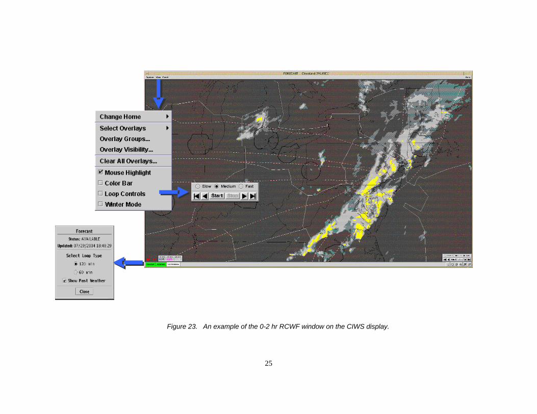
(TCWF) for ITWS is displayed in a new window type capable of animation. The TCWF animated loop contains 30 minutes of past weather, the current weather, and up to 60 minutes of forecast weather, in 10-min increments. The Regional Convective Weather Forecast (RCWF) display for CIWS provides a similar animated loop, but with 60 minutes of past weather, the current weather, and up to 120 minutes of forecast weather, in 15-min increments. Figure 22 shows an example of the ITWS TCWF display and Figure 23 shows an example of CIWS RCWF display. Features of both CWF displays include user selectable loop preferences such as: pausing the loop to look at single static time images, displaying past weather, selecting the forecast loop time-horizon, as well as changing the speed of the loop. Forecast accuracy scores and verification contours are also available on the SD (see Section 3.5).
There are several aspects of the 0-2 hr
Forecast that can be displayed in various CIWS windows, as illustrated in Figure 24. First, the past forecast performance can be displayed graphically via forecast verification contours overlaid on the past weather portion of the loop in the Forecast window. Second, the 30, 60, and/or 120-min forecast can be represented via color-coded overlay contours on the VIL Precip mosaic in the
NEXRAD window. This provides users with a very useful “shorthand” forecast when they only have time to glance at the Precip display. Third, also in the NEXRAD window, it is possible to overlay a map of the Growth and Decay Trends mosaic. This information, used internally in CWF to generate the 0-2 hr Forecast loop, provides users with an ever-vigilant diagnosis of recent storm behavior. Knowing that a cluster of cells is growing – even if the storms do not currently appear threatening – can provide important tactical guidance for route management and short-term planning. Finally, the CIWS display of Echo Tops, used internally in the CWF Weather Classification algorithm, provides a valuable tool for enroute traffic flow management. An Echo Tops Forecast as a derivative of the CWF technology is currently under development (see Section 5.2.2).
New York users in particular have expressed
concerns about the utility of the CWF display during weak (in terms of radar reflectivity) yet operationally significant precipitation events (e.g., east coast snow storms, hurricane remnants inland, etc.). Not only does the standard 6-level color scale fail to represent the important storm features embedded within level 1, but the forecast and scoring of the level 3+ regions makes little sense in these scenarios.
In response to this feedback, the CWF
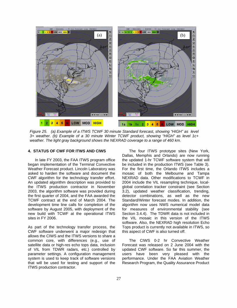
forecast is now available in two modes: Standard and Winter (Figure 25). In Standard mode, precipitation levels 1-6 are shown. Standard forecasts are displayed in three levels: low (shown in dark gray), moderate (shown in light gray), and high (shown in yellow) to represent the level 3+ weather forecast. In Winter mode, the bottom threshold for level 1 precipitation is lowered to reveal more weak precipitation and the whole interval is further divided into levels 1a, 1b, and 1c, while levels 2-6 remain unchanged. In Winter mode, the high forecast is for level 1c+ weather. The Winter Forecast (Fig. 25b) better reveals the relative precipitation strengths of the weather in central New York state than does the Standard Forecast (Fig. 25a). Both the Airport/Regional scoring numbers and the verification contours relate to the high forecast being shown. For the Standard forecast, this is the Level 3+ region; for the Winter Forecast, this corresponds to the Level 1c+ region.

24
ITWS Alerts
Display Configuration Buttons
Product Status Buttons
Forecast LoopDisplay Window
PrecipitationDisplay Window
Window Window Configuration Configuration
ButtonsButtons
ITWS AlertsITWS Alerts
Display Configuration Buttons
Product Status Buttons
Forecast LoopDisplay Window
PrecipitationDisplay Window
PrecipitationDisplay Window
Window Window Configuration Configuration
ButtonsButtons
Figure 22. An example of 0-1 hr TCWF Window on the New York ITWS Situation Display.
25
Figure 23. An example of the 0-2 hr RCWF window on the CIWS display.

26
Figure 24. Example of the CIWS display showing forecast and echo tops information. The 60-min forecast verification contours are shown in the Forecast window (upper left), overlaid on the current precipitation. The 30, 60 and/or 120 min forecast can be viewed in the NEXRAD window via color-coded contours (upper right); shown is the white 120-min forecast. The Growth & Decay Trends can also be viewed as an overlay in the same window with orange representing growth and blue - decay; here they are shown overlaid on the satellite data with the Precip turned off (lower right). The Echo Tops information, used internally in the CWF algorithm, is also shown (lower left).
27
4. STATUS OF CWF FOR ITWS AND CIWS
In late FY 2003, the FAA ITWS program office
began implementation of the Terminal Convective Weather Forecast product. Lincoln Laboratory was asked to harden the software and document the CWF algorithm for the technology transfer effort. An updated algorithm description was provided to the ITWS production contractor in November 2003, the algorithm software was provided during the first quarter of 2004, and the FAA awarded the TCWF contract at the end of March 2004. The development time line calls for completion of the software by August 2005, with deployment of the new build with TCWF at the operational ITWS sites in FY 2006. As part of the technology transfer process, the CWF software underwent a major redesign that allows the CIWS and the ITWS versions to share a common core, with differences (e.g., use of satellite data or high-res echo tops data, inclusion of VIL from TDWR radars, etc.) controlled by parameter settings. A configuration management system is used to keep track of software versions that will be used for testing and support of the ITWS production contractor.
The four ITWS prototype sites (New York,
Dallas, Memphis and Orlando) are now running the updated 1-hr TCWF software system that will be included in the production ITWS (see Table 3). For the first time, the Orlando ITWS includes a mosaic of both the Melbourne and Tampa NEXRAD data. Other modifications to TCWF in 2004 include the VIL resampling technique, local- global correlation tracker constraint (see Section 3.2), updated weather classification, trending, detector combinations, as well as the new Standard/Winter forecast modes. In addition, the algorithm now uses NWS numerical model data for measures of environmental stability (see Section 3.4.4). The TDWR data is not included in the VIL mosaic in this version of the ITWS software. Also, the NEXRAD high resolution Echo Tops product is currently not available in ITWS, so this aspect of CWF is also turned off.
The CIWS 0-2 hr Convective Weather
Forecast was released on 2 June 2004 with the updated CWF software. So far this summer, the users have been very pleased with the performance. Under the FAA Aviation Weather Research Program, the Quality Assurance Product
(a) (b)(a) (b)
(a) (b)
Figure 25. (a) Example of a ITWS TCWF 30 minute Standard forecast, showing “HIGH” as level 3+ weather. (b) Example of a 30 minute Winter TCWF product, showing “HIGH” as level 1c+ weather. The light gray background shows the NEXRAD coverage to a range of 460 km.

28
Table 3. Implementation dates for the redesigned TCWF software at the ITWS
prototype sites.
Development Team (QAPDT) monitors the statistical performance of the CIWS 0-2 hr Tactical CWF algorithm, along with the National Convective Weather Forecast, the NCAR Autonowcaster and, under separate sponsorship, the Collaborative Convective Forecast Product (Mahoney et al., 2002). Lincoln Laboratory asked that the QAPDT produce graphical comparisons of the CWF vs. the truth for the 30, 60 and 120 min forecasts, in addition to their usual statistics. An example of their password-protected web page is shown in Figure 26. Our intent is to further update the CIWS CWF in Fall, 2004 with the Winter/Standard mode selection capability. 5. FUTURE WORK
The CWF algorithm has improved greatly since its debut in Dallas in 1998, but there are still areas of relatively poor performance for the 0-2 hr forecast. For example, the forecast fails to decay airmass cells properly as they move offshore, either off the east coast or over Lake Michigan. Inclusion of land-sea surface temperatures in the Final Forecast Combination will be helpful. Also, the CWF algorithm can currently grow an existing storm, but cannot anticipate convective initiation. Without this, forecasts of convectively active regions will deteriorate rapidly with forecast time horizon. This is an area of intense research for the Convective Weather PDT, as described in Section 5.1, below. Further improvements are also demanded by the desire to couple the forecast data with automated air traffic management tools currently under development. Work to develop an accurate error model for the forecast and to anticipate the future storm echo tops is underway, and is also described below (Section 5.2). Finally, extending the forecast lead time beyond 2 hrs will require at least guidance from numerical models if not an explicit precipitation forecasts. Future work in this area is described in Section 5.3.
5.1 Including Convective Initiation One of the largest sources of error in the
current 0-2 hour Convective Weather Forecast is its inability to accurately account for new convective storm development. Figure 27 depicts a perfect forecast of the rapidly developing convection in Illinois, Wisconsin and around Lake Michigan on 3 August 2003, compared with the actual CIWS forecast for that same time. Clearly the CWF under-forecast the amount of precipitation by failing to initiate new convection in the region.
In many situations convective initiation is
preceded by low altitude convergence in the horizontal winds (e.g., Wilson and Megenhardt, 1997, Wilson et al., 1998). Gridded wind analyses that utilize Doppler weather radar, surface observations, and aircraft measurements are the best source of low altitude winds. The Convective Weather PDT has underway an experiment to demonstrate that high resolution (1-5 km) boundary layer wind analyses can be generated in real time over large domains (i.e. 500 km or greater).
An initial feasibility study utilizing a domain
centered near Chicago, IL demonstrated boundary layer wind synthesis using the ITWS Terminal Winds technique. Preliminary results from the August 3rd case indicate this technique can be utilized over the large domain in what is equivalent to a single Doppler retrieval mode, and provide a suitable wind analysis for identifying low altitude coherent structures in the wind field (Figure 28). The results were surprisingly good in this lake breeze case considering the weak divergence signatures, complexity of the case, and the minimal post processing conducted on the 1 km resolution wind analysis. As a result of this and other encouraging preliminary analyses, a prototype large-scale Terminal Winds analysis system will be tested in real-time. The NCAR Auto-Nowcaster and four-dimensional variational wind retrieval system are also being tested in the same domain (Saxen et al., 2004; Sun and Crook, 2001). Also, experiments to determine the value of including GOES satellite data in the convective initiation forecast are being conducted as well.
ITWS Site New TCWF Implementation Date
New York 13 May 2004
Memphis 5 August 2004
Orlando 12 August 2004
Dallas 25 August 2004

29
Figure 26. Example of web-based graphics from the off-line forecast verification exercise conducted by the Quality Assurance Product Development Team. The green areas represent hits, the red - false alarms, and the blue – missed detections. This example shows the 1-hr CIWS Tactical Convective Weather Forecast verified at the level 2 precipitation threshold (Scaled VIL=73). Notice that the bulk of the heavy weather in Michigan and northern Indiana/Ohio is forecasted very well, but that the initiation of small airmass storms in southern Illinois/Indiana is largely missed, and the algorithm failed to decay the weather off the east coast.
Perfect 60-min Forecast CWF 60-min ForecastPerfect 60-min Forecast CWF 60-min Forecast Figure 27. A “perfect” 60-min convective weather forecast (left) vs. the CWF (right) for lake breeze-induced and land-based airmass convection on 3 August 2003. This comparison illustrates the large errors that can occur because convective initiation is not included in CWF.

30
Once the boundary layer wind synthesis has been performed, as described in the preceding section, the question of automatic boundary detection can be addressed. Lincoln Laboratory has developed the Machine Intelligent Gust Front Algorithm (MIGFA), which uses polar surface reflectivity and velocity radar input to identify and track convergence boundaries automatically (Morgan and Troxel, 2002). MIGFA does this by forming a set of so-called “interest images”, which indicate the likelihood that a convergence boundary passes through a given pixel in the radar data space.
Figure 28. Wind vectors and six level weather radar reflectivity returns valid at 19:00 UTC on 3 August 2003. The wind vectors are from the 900 mb level of the TWINDS large domain 1-km wind analysis. The wind analysis captures realistic low altitude convergence signatures associated with the lake breeze and convection.
A key point is that MIGFA-style analysis is not limited to just polar radar reflectivity and velocity data. Any data relevant to boundary structures can be directly employed by MIGFA, if that data is first “converted” into the interest/orientation image format used by MIGFA. For example, MIGFA-style feature detectors for “convergence” and “dispersal” can be run on the wind grid, thus determining the likely locations and orientations of any boundaries in the synthesized wind field. This data can then be fed into MIGFA's extraction and tracking modules in exactly the same way as MIGFA's existing interest images are currently
used. In fact, improvement in MIGFA performance over that based on single-radar polar input is expected because of the wind synthesis technique’s ability to analyze multiple radars simultaneously, and to capture boundary layer convergence signatures in locations where there may be very few radar returns. MIGFA will be tested on the synthesized wind grids in FY 2005.
5.2 Coupling Forecasts to ATM Automation Tools
Through discussions with the developers of Air
Traffic Management (ATM) automation tools such as Mitre’s User Request Evaluation Tool (URET; Heagy and Kirk, 2003), and the New York Route Availability Planning Tool (RAPT; Allan et al., 2004), the need for additional tactical forecast capabilities has become clear. First, the need to produce a finer time granularity has been addressed. The CIWS 0-2 hr CWF is now available in 5 min time increments, although the user display still shows only the 15-min interval loop. Aircraft travel time and routing is so fast that storms must be resolved with the 5-min granularity to correctly judge route impacts. Second, a spatial error estimate as a companion to the deterministic forecast is required to convey the uncertainty in predicted route blockage, and to stabilize the route blockage assessment (Section 5.2.1). Finally, departing aircraft reach enroute flight levels quickly, and enroute flights in general will be blocked only by storms that extend above ~25Kft. Thus a forecast of storm echo tops is also highly desirable (Section 5.2.2).
5.2.1 Forecast Error Model In addition to a deterministic forecast of the
VIL value expected at a given pixel, users of the CWF system, especially automation tools that can digest large grids of information, also need the estimated variance of the VIL forecast at each pixel. This estimate can be obtained from an empirical analysis of historic data spanning a range of seasons and locales, and/or from statistics gathered in real-time on the day in question. The variance of the forecast is modeled as a function of the forecast time horizon and the local variability of the weather at the time the forecast is issued.
The precision of the forecast is a decreasing
function of forecast time horizon. This is illustrated at the top of Figure 29 with scattergrams of Forecast VIL values vs. Truth VIL values for a 5

31
minute forecast (left) and a 1 hour forecast (right). As expected, the 5-min forecast has less scatter (increased precision) relative the to 1 hour forecast. The corresponding histograms of the resulting VIL values when a forecast was made for VIL at the Level 3 precipitation threshold (scaled VIL = 128) are shown at the bottom of Figure 30. These VIL=128 forecasts represent a cross-section of statistics along the horizontal black line in the middle of the scattergrams. Again, as expected, the standard deviation of the forecast increases with increasing forecast time horizon.
The variance of the forecast is not a function
of the forecast time horizon alone, but also a function of the local variability of the weather itself. This can be seen by classifying forecasts according to the local variability of the weather. Similar scattergrams and histograms to those shown in Figure 30 can be produced comparing
forecasts of weather to truth for low variability and for high variability weather.
To overcome the increasing variance of the
forecast as the forecast time and local variability increase, we can compute spatially-averaged forecasts. These area-averaged forecasts will have greater precision (lower relative standard deviation) compared with single pixel deterministic forecasts. Figure 30 shows the effects of increasing the amount of spatial averaging upon the scattergram of the 1-hr Forecast VIL vs. Truth VIL and the corresponding histograms of the 1-hr, VIL = 128 forecast. These plots show that the standard deviations do indeed decrease as the amount of spatial averaging is increased.
Figure 29. Scattergrams (top) of forecast VIL value vs. truth VIL value for a 5 min forecast (left) and a 1-hr forecast (right). Histograms (bottom) of the resulting VIL values for a forecast of level 3 precipitation (VIL = 128; corresponding to the horizontal black line in scattergrams) at 5 min (left) and 1-hr (right).

32
Figure 30. Scattergrams of forecast vs. truth VIL (top) and histograms at forecast VIL=128 (bottom) for varying size of averaging box.
In general, we can compute the minimum averaging box required to achieve a stated level of precision (standard deviation). Figure 31 shows the width of the averaging box required to achieve a stated standard deviation as forecast time horizon increases. Germann and Zawadzki (2004) studied large scale continental storms at forecast time horizons out to 8 hrs, and also developed a notion of optimum scale vs. forecast time horizon. The study here focuses in detail on the 0-2 hr forecast time range, which the large-scale study did not precisely address.
By providing an accurate estimate of the error
variance of each forecast pixel along with the VIL value itself, developers of ATM automation tools can create probabilistic estimates of route blockage. These will prevent route status from changing rapidly from “blocked” to “clear” as each refresh of the CWF is incorporated. Research to produce and utilize the CWF error model is ongoing at Lincoln Laboratory.
5.2.2 Echo Tops Forecasts Operational experience from the Corridor
Integrated Weather System has shown that an accurate and timely Echo Tops mosaic is a critical Air Traffic Management tool. While the Growth and Decay Trends overlay is helpful to users in predicting a growing top, the decay products have not been very useful in detecting or predicting decaying storm tops. Often ATM users make mental notes of decaying trends of tops and anticipate the opening of a route in the 1-2 hour time frame. In coupling the CWF with tools that help alleviate the mental workload of the ATM personnel and provide improved situational awareness, we are actively researching how to produce and deploy an Echo Tops Forecast product as part of CWF for the CIWS system. Operationally, a prediction of echo tops requires most accuracy in the range of 25-35 Kft to correctly predict aircraft thunderstorm avoidance behavior.

33
Figure 31. Curves of constant standard deviation (scaled VIL units) plotted against Forecast Time Horizon (min) and Width of Averaging Box (km).
Several approaches to forecasting echo tops are being considered, including a) Echo Tops advection coupled with precipitation trends to produce a heuristic rule-based algorithm, b) trending of Echo Tops heights, and c) development of multiple regression models using predictors such as precipitation, cell size, echo tops and other potentially significant meteorological variables.
Developers of the Route Availability Planning Tool (RAPT; Allan et al., 2004) have been studying the use of echo top trending coupled with precipitation forecasts and RUC convective cloud top potential to produce up to a 1-hr Echo Tops prediction. These efforts are being coupled with an advection-based Echo Tops forecast developed under the CWF system and the results are currently being evaluated.
5.3 Coupling Forecasts with NWP Models
The use of the CWF tracking and trending
techniques described in this paper are most accurate and appropriate in the 0-2 hr forecast interval. Over even this short interval, the skill of these heuristic techniques diminishes exponentially with increasing time horizon. The
Convective Weather PDT is exploring methods for improving the overall forecast accuracy by incorporating information derived from Numerical Weather Prediction (NWP) model forecasts.
When mesoscale numerical models run at resolutions in which individual convective elements are explicitly resolved, they have demonstrated skill in reproducing observed storm life cycles, structures, and other properties of individual and grouped convective storms. Figure 32 shows a mesoscale NWP simulation of the lake breeze initiation case mentioned in Section 5.1, which results in good timing and spatial extent of the thunderstorm initiation. NWP simulations have also been useful in characterizing convection in idealized modeling studies (Weisman and Klemp, 1982, 1984, 1986; Droegemeier, 1990). Unfortunately, most often the inaccuracies in the timing and spatial representation of convective precipitation in NWP models make their direct coupling with heuristic-based automated convective weather forecasts extremely difficult (Brooks et al., 1992).

34
11:00 am 12:00 noon 1:00 pm 2:00 pm
3 August 2003Init. at 3:00 am
11:00 am 12:00 noon 1:00 pm 2:00 pm
3 August 2003Init. at 3:00 am
To effectively couple CWF forecasts with NWP
forecasts, the NWP forecast elements that are robust must be exploited while, as the same time, the characteristic inaccuracies must be avoided. This is a new area of development and we are just beginning to examine its potential. The first step involves identifying elements of the mesoscale NWP forecast that provide accurate information on convective behavior without association with a specific temporal or spatial location. In particular, the mesoscale model forecasts are analyzed with image processing software to diagnose and characterize variables such as: preferred orientations for the convection, aerial coverage of precipitation, precipitation intensity trends, storm motions, storm mode/type, etc. as a function of time. These NWP-derived properties are matched with the observed properties to identify the temporal correlations. These correlations can then be used to shift the NWP information in time (and space) to maximize its accuracy. The aligned convective weather properties are ingested by the CWF system and allowed to have an increasing influence on the automated forecast as the forecast length increases.
6. SUMMARY
This paper has discussed the development
history and the algorithmic details of the FAA Tactical 0-2 hr Convective Weather Forecast capability. The CWF has been used in both the ITWS (1-hr forecast) and CIWS (2-hr forecast) proof-of-concept demonstrations, and has proven highly useful in these operational settings as an aid to tactical traffic flow management. Keeping in mind the annual air traffic delay statistics curves, we recognize that the CWF technology – as valuable as it may be for making short-term
forecasts - does nothing to solve the national summertime delay problem if air traffic management decisions are not being made differently as a result. So while a major milestone was reached in 2004 with the transfer of the CWF technology to the ITWS program for implementation, work is ongoing to improve the performance and increase the operational utility of the CWF.
7. REFERENCES Allan, S., R. DeLaura, B. Martin, D. Clark, C. Gross, and
E. Mann, 2004: Advanced Terminal Weather Products Demonstration in New York, 11th Conference on Aviation, Range, and Aerospace Meteorology, Hyannis, MA.
Brooks, H. E., C.A. Doswell, R.A. Maddox, 1992: On the Use of Mesoscale and Cloud-Scale Models in Operational Forecasting. Weather and Forecasting, Vol. 7, pp. 120–133.
Cartwright, T.J., M.M. Wolfson, B.E. Forman, R.G. Hallowell, M.P. Moore, and K.E. Theriault, 1999: The FAA Terminal Convective Weather Forecast Product: Scale Separation Filter Optimization, 29th International Conference on Radar Meteorology, Montreal, Quebec, pp. 852-855.
Chornoboy, E.S., A.M. Matlin, and J.P. Morgan, 1994: Automated Storm Tracking for Terminal Air Traffic Control, MIT Lincoln Laboratory Journal, No. 7, pp. 427-448.
Crowe, B.A and D.W. Miller, 1999: The Benefits of Using NEXRAD Vertically Integrated Liquid Water as an Aviation Weather Product. 8th Conference on Aviation, Range, and Aerospace Meteorology, Dallas, Texas, pp. 168-171.
Delanoy, R. L., J.G. Verly, and D. Dudgeon, 1992: Functional Templates and Their Applications to 3-D Object Recognition, Proc. Int. Conf. On Acoustics, Speech, and Signal Processing (ICAASP), 3, IEEE, pp. III-141-144.
Figure 32. Time series of NWP-generated VIL precip maps for the 3 August 2003 lake breeze convective initiation case discussed in Section 5.1, and shown in Figures 27 and 28. This shows an example where the MM5 mesoscale model generated quasi-realistic convection around the lake at approximately the right time, from a single run initialized with large scale environmental conditions at 3 am local time.

35
Droegemeier, K. K., 1990: Toward a science of storm-scale prediction, 16th Conference on Severe Local Storms. Kananaskis Park, Alberta, Canada. Amer. Meteor. Soc. 256-262.
Dupree, W.J., R.J. Johnson, M.M. Wolfson, K.E. Theriault, B.E. Forman, R.A. Boldi, and C. A. Wilson, 2002: Forecasting Convective Weather Using MultiScale Detectors and Weather Classification – Enhancements to the MIT Lincoln Laboratory Terminal Convective Weather Forecast, 10th Conference on Aviation, Range, and Aerospace Meteorology, Portland, Oregon, pp. 132- 135.
Evans, J.E., K. Carusone, M. Wolfson, M. Robinson, E. Ducot, B. Crowe, 2004: Improving Convective Weather Operations in Highly Congested Airspace with the Corridor Integrated Weather System (CIWS), 11th Conference on Aviation, Range and Aerospace Meteorology, Hyannis, MA
FAA DOT Communication/Navigation/Surveillance, Engineering and Test Division, Weather Branch, ACT-320, 2001: Terminal Convective Weather Forecast (TCWF) 2000 Demonstration Report, 40 pp. and appendices.
Forman, B.E., M.M. Wolfson, R.G. Hallowell, M.P. Moore, 1999: Aviation User Needs for Convective Weather Forecasts, 8th Conference on Aviation, Range and Aerospace Meteorology, Dallas, TX, Jan.10-15, pp. 526-530
Germann, U. and I. Zawadzki, 2004: Scale Dependence of the Predictability of Precipitation from Continental Radar Images. Part II: Probability Forecasts, J. Appl. Meteor., Vol. 43, pp. 74-89.
Heagy, W. and Kirk, D., 2003: Description of URET Enhancements to Support Severe Weather Avoidance, AIAA-ATIO, Denver, CO.
Mahoney, J.L., J.K. Henderson, B.G. Brown, J.E. Hart, A. Loughe, C. Fischer, and B. Sigren, 2002: The Real-Time Verification System (RTVS) and its Application to Aviation Weather Forecasts. 10th Conference on Aviation, Range, and Aerospace Meteorology, 13-16 May, Portland, OR.
MCR Federal, Inc., 2001: FAA Terminal Convective Weather Forecast Benefits Analysis Report, No. TR-7100/029-1. 31 pp.
Megenhardt, D., C.K. Mueller, N.A. Rehak, S.B. Trier, and D. Ahijevych, 2004: NCWF-2 Probabilistic Forecasts. 11th Conf. on Aviation, Range, and Aerospace Meteorology, Hyannis, MA
Morgan, J. and S. Troxel, 2002: CSKETCH Image Processing Library, Project Report ATC-283, MIT Lincoln Laboratory, 183 pp.
Robinson, M, J.E. Evans, and B.A. Crowe, 2002: Enroute Weather Depiction Benefits of the NEXRAD Vertically Integrated Liquid Water Product Utilized by the Corridor Integrated Weather System. 10th Conf. on Aviation, Range, and Aerospace Meteorology, Portland, OR.
Robinson, M., J. Evans, B. Crowe, D. Klingle-Wilson and S. Allan, 2004: CIWS Operational Benefits 2002-3: Initial Estimates of Convective Weather Delay Reduction, MIT Lincoln Laboratory Project Report ATC-313, 326 pp.
Saxen, Thomas R., C.K. Mueller, J. Wilson, R. Roberts, E. Nelson, D. Ahijevych, and S. Trier, 2004: Updates to the NCAR Auto-nowcaster for the 2004 convective weather season.11th Conf. on Aviation, Range, and Aerospace Meteorology, Hyannis, MA.
Smalley, D. J., and B.J. Bennett, 2002: Using ORPG to Enhance NEXRAD Products to Support FAA Critical Systems. 10th Conf. on Aviation, Range, and Aerospace Meteorology, Portland, Oregon.
Sun, J. and N.A. Crook, 2001: Real-time low-level wind and temperature analysis using single WSR-88D data. /Wea. Forecasting, 16, pp. 117-132.
Theriault, K.E., M.M. Wolfson, B.E. Forman, R.G. Hallowell, M.P. Moore, R.J. Johnson, Jr., 2000: FAA Terminal Convective Weather Forecast Algorithm Assessment. 9th Conf. on Aviation, Range, and Aerospace Meteorology, Orlando, FL.
Theriault, K.E., M.M. Wolfson, W.J. Dupree, B.E. Forman, R.G. Hallowell, R.J. Johnson and M.P. Moore, 2001: TCWF Algorithm Assessment – Memphis 2000, MIT Lincoln Laboratory Project Report, ATC-297, 109 pp.
Weisman, M.L., and Klemp, J.B. 1982: The Dependence of Numerically Simulated Convective Storms on Vertical Wind Shear and Buoyancy. Monthly Weather Review, Vol. 110, pp. 504–520.
Weisman, M.L., Klemp, J. B. 1984: The Structure and Classification of Numerically Simulated Convective Storms in Directionally Varying Wind Shears. Monthly Weather Review, Vol. 112, pp. 2479–2498.
Weisman, M.L., and J.B. Klemp, 1986: Characteristics of isolated convective storms, Mesoscale Meteorology and Forecasting, P. S. Ray Ed., American Meteor. Soc., pp. 331-358.
Wilson, J.W. and D.L. Megenhardt, 1997: Thunderstorm Initiation, Organization, and Lifetime Associated With Florida Boundary Layer Convergence Lines. Monthly Weather Review, Vol. 125, pp. 1507–1525.
Wilson, J.W., Crook, N.A., Mueller, C.K., Sun J. and M. Dixon, 1998: Nowcasting Thunderstorms: A Status Report, Bulletin of the American Meteorological Society, Vol. 79, pp. 2079-2099.
Wolfson, M.M., B.E. Forman, R.G. Hallowell, and M.P. Moore, 1999: The Growth and Decay Storm Tracker, 8th Conference on Aviation, Range, and Aerospace Meteorology, Dallas, TX, pp.58-62.
Wolfson, M., R. Boldi, K. Calden, W. Dupree, B. Forman, R. Johnson, Jr., E. Mann, and C. Wilson, 2004: ITWS Pre-Planned Product Improvement Algorithm Description for Convective Weather Forecast, Project Report ATC-316, MIT Lincoln Laboratory, 476 pp.