3. synthetic cdos of cdos - idc · lehman brothers | quantitative credit research quarterly 30 june...

Synthetic CDOs of CDOs: Squaring theDelta-Hedged Equity Trade

Tight spreads in the credit markets have forced investors to turn to innovative structures in the search for yield.

One such structure is the synthetic CDO of CDO tranches, also known as CDO2. In this article, we introduce this

structure, present a framework for valuation, and highlight the risk-return profile of a delta-hedged equity super

tranche referencing a portfolio of mezzanine CDO tranches.

Prasun Baheti, Roy Mashal, Marco Naldi and Lutz Schloegl

Fixed IncomeQuantitative Credit Research

30 June 2004

Lehman Brothers | Quantitative Credit Research Quarterly

30 June 2004 1

Synthetic CDOs of CDOs: Squaring the Delta-Hedged Equity Trade Tight spreads in the credit markets have forced investors to turn to innovative structures in the search for yield. One such structure is the synthetic CDO of CDO tranches, also known as CDO2. In this article, we introduce this structure, present a framework for valuation, and highlight the risk-return profile of a delta-hedged equity super tranche referencing a portfolio of mezzanine CDO tranches.

1. INTRODUCTION

In the past few years, dynamically hedged synthetic CDO tranches have had an impact on the credit derivatives market which is difficult to overstate. They have increased the liquidity and changed the dynamics of the default swap market via the “synthetic bid” for credit, and taken the CDO concept beyond the realm of structured finance into the derivatives arena. Nevertheless, synthetic CDOs are susceptible to arbitrage spreads just like their cashflow counterparts. Given the relentless spread tightening since the end of 2002, it is perhaps not surprising that it has become more difficult to obtain the yields investors had become used to via standard synthetic tranches.

The CDO2 concept addresses this difficulty by providing an additional layer to the capital structure. In a CDO2, a portfolio of synthetic CDO tranches is itself tranched into so-called super tranches. This introduces quite a few new variables into the structuring equation. Not only is the composition of the underlying portfolio of individual tranches to be determined, but their joint characteristics can be tailored by varying the degree of overlap between the reference credits in the individual pools. Moreover, extra flexibility is provided to the structure by the ability to choose the level of subordination and the width of the super tranche. These additional degrees of freedom make it possible to further fine tune the risk-return profile of a loss tranche, eg, achieving high leverage while controlling the exposure to idiosyncratic default risk.

CDOs of CDOs have been used for some time in the cashflow world. However, the terms of the purely synthetic CDO2 we are discussing here are somewhat different, so that it is worth clarifying the structure and the notation in section 2. In section 3, we extend the semi-analytical techniques for synthetic tranche valuation to the CDO2 case, and in section 4 we illustrate the flexibility of super tranches by means of an application to a delta-hedged equity trade.

Prasun Baheti Tel: +1-212-526-9251

[email protected]

Roy Mashal Tel: +1-212-526-7931

[email protected]

Marco Naldi Tel: +1-212-526-1728

[email protected]

Lutz Schloegl Tel: +44-20-7102-2113

[email protected]


30 June 2004 2

2. THE CDO2 STRUCTURE

The fundamental inputs to a CDO2 trade are a large pool of individual credits. The main constraint on the size of the pool is the number of credits that can be dynamically hedged due to their liquidity in the single-name default swap market. A typical pool might consist of 250-350 credits.

We denote the total number of credits in the pool by M. The credits are assigned to different so-called “mini portfolios”, and we denote the total number of mini portfolios by N. It is important to note that a given credit can appear in more than one portfolio, and that the weight of a particular credit is specific to each mini portfolio.

Source: Lehman Brothers.

The percentage weight of credit j in mini portfolio k is denoted by wj,k; these weights are constrained to be non-negative and add up to 100% within each mini portfolio, ie:

∑ ===

==≥M

j kj

kj

Nkw

NkMjw

1 ,

,

.,...,2,1 ,1

,,...,2,1 ,,...,2,1 ,0

The matrix ( )kjw , is the “population matrix” of the trade; it encapsulates the information

about issuer concentrations and the overlap between different mini portfolios.

As the underlying risk sources of the CDO2, we consider a tranche linked to each mini portfolio. The easiest way to describe the kth mini tranche is by its percentage subordination U k, and its percentage width V k. Note that so far we have not fixed any absolute notional amounts yet. We denote the absolute notional of the kth mini tranche by N k, so that the total notional of the corresponding mini portfolio is N k/V k. This will become relevant when we describe how the individual credit losses flow through to the super tranche.

The portfolio underlying the super tranche consists of the N mini tranches, and its total

notional is therefore∑ =

N

kkN

1. The super tranche itself is described by its percentage

subordination U st and percentage width V st. We also refer to the portfolio of mini tranches as the super portfolio.


30 June 2004 3

Let us now consider how the credit losses in the pool ultimately flow to the super tranche. Suppose that credit j defaults with a recovery rate of R. The loss to the kth mini portfolio is then given by ( ) kk

kj VNwR /1 ,− , and the percentage notional lost is equal to ( ) kjwR ,1− .

Once the cumulative percentage loss in any of the mini portfolios is greater than its tranche subordination, the super portfolio starts to take losses and the subordination of the super tranche is reduced. The seller of super tranche protection is obliged to make protection payments once the tranche has been eaten into, just as in a standard synthetic CDO tranche. Similarly, the contractual spread paid to the protection seller is based on the outstanding notional of the super tranche. Note that the synthetic super tranche structure is different from traditional cash CDOs of CDOs in that the mini tranches are not “physical” assets as such. They have no premium associated with them and only serve to define the subordination structure to resolve losses.

As we explain in greater detail in the next section, valuation can be performed using the concept of “tranche curve”. To construct this curve, we need to define the cumulative percentage loss of the super tranche Lst up to a given time horizon. If the cumulative percentage loss to the kth mini portfolio is L k, then the cumulative percentage loss to the kth mini tranche is:

[ ] ( )[ ]k

kkkkkkmt

VVULULL

+++−−−=)(

The cumulative percentage loss to the super portfolio is therefore:

∑

∑

=

== N

kk

N

kkmtk

sp

N

LNL

1

1)(

,

and the cumulative percentage loss to the super tranche is:

[ ] ( )[ ]st

ststspstspst

VVULULL

+++−−−=

While the loss on a standard CDO tranche is a call spread on the underlying portfolio loss, the equations above show that the super tranche loss is given by compound options, effectively calls on a basket of vanilla call spreads.

3. A SIMPLE MODEL FOR VALUATION

At the core of any CDO pricing model is a mechanism for generating dependent defaults. Latent variable models describe default as an event generated by a latent variable – generally interpreted as asset return – falling below a specified threshold, which is in turn calibrated to observable CDS spreads of the reference credit. The dependence among the default times of different names is then naturally determined by the dependence structure (a.k.a. the copula) of the latent variables.

One of the most popular latent variable models combines a Gaussian copula with a one-factor correlation framework. The return of asset j, Xj, is driven by a common market factor Y, and an idiosyncratic variable Ej:

.1 2jjjj EYX ⋅−+⋅= ββ


30 June 2004 4

Here the variables Y, Ej , j=1,2…,M are taken to be independent standard normal random variables, so that the asset returns Xj are jointly normal with an MxM correlation matrix given by:

( ) ( )ljljC ββ ⋅=, .

Within the one-factor Gaussian framework, the dependence structure is fully specified by a vector of betas, each of which can be interpreted as the correlation of an asset with the market. Given a particular realization of the market factor, the probability that the jth credit defaults is now given by:

( ) [ ] ,1

|2

−

⋅−=<=

j

jjjjj

YDNYDXPY

ββ

π

where Dj represents the default threshold for a given time horizon calibrated to the jth name’s credit curve.

The parsimonious one-factor structure of this model implies that, conditional on the realization of the market factor, the M individual credits are independent. When pricing a standard CDO, this conditional independence greatly facilitates the calculation of the conditional loss distribution of the tranche. In a CDO2, however, since some of the credits may belong to several mini portfolios, the loss distributions of the mini tranches need not be conditionally independent even if the defaults of the individual credits are. The possibility of overlapping credits in the reference mini portfolios significantly complicates the task of recovering the conditional joint loss distribution of the mini tranches, which is in turn necessary to compute the conditional loss distribution of the super tranche. In the Appendix, we show how we can overcome this obstacle by means of a recursive procedure which is a multivariate extension of a well-known recursive algorithm used for standard CDOs.

Once we know how to compute the loss distribution of the super tranche for a given realization of the market factor, it is straightforward to take a probability weighted average across all possible market realizations and thus recover the unconditional loss distribution of the super tranche. Repeating the entire procedure for a grid of horizon dates, and interpreting the expected percentage loss up to time t as a cumulative default probability, we can price a tranche using exactly the same analytics as in a single-name default swap. More precisely, define the “survival probability” of the super tranche up to time t as:

[ ]stt

st LEtQ −= 1)( .

Then the two legs of the CDO2 swap can be priced using:

PV(Protection Leg) = ∑=

− −S

ii

sti

sti

st sQsQsBN1

1 ))()()(( ,

PV(Premium Leg) = ∑=

∆T

iii

sti

stst tBtQNc1

)()( ,

where cst is the coupon paid on the super tranche, Nst is the notional of the super tranche, ti, i=1,2,…,T are the coupon dates, ∆i, i=1,2,…T are accrual factors, si, i=1,2,…,S discretize the timeline for the valuation of the protection leg, and B(t) is the risk-free discount factor for time t.

To summarize, in the context of a one-factor Gaussian framework, we can price a super tranche if we specify:


30 June 2004 5

1. the CDO2 structure, ie,

a. the population matrix ( )kjw , ,

b. the mini tranches triples ( )kkk NVU ,, ,

c. the super tranche triple ( )ststst NVU ,, ,

2. the issuer curves of all the underlying credits (used to calibrate the thresholds Dj, j=1,2,…,M for each horizon date),

3. the asset correlations among all of the underlying credits (used to calibrate the market sensitivities βj, j=1,2,…,M).

The major advantage of the pricing approach outlined above is that the quasi-analytic valuation is convenient for the computation of precise sensitivities to the underlying parameters. As we show in the next section, these sensitivities can be highly valuable for the purpose of hedging out some of the risks and designing attractive risk-return profiles.

4. DELTA-HEDGING SYNTHETIC TRANCHES

A trade that has recently gained popularity consists of selling protection on a synthetic equity tranche and simultaneously buying protection on the individual CDS of the underlying names. Single-name protection is bought in amounts sufficient to delta-hedge the tranche position against individual spread movements, ie, to immunize the present value of the long position in the equity tranche against small changes in the underlying spread curves.

Selling delta-hedged equity protection provides the investor with a risk-return profile which generally displays positive carry, negative “Value On Default” (VOD), positive systematic convexity, and positive exposure to correlation risk. In other words, the investor earns positive carry and profits from general spread volatility through the positive convexity. In return for these features, she tolerates exposure to idiosyncratic default risk and to changes in correlations. We will come back to each of these points in greater detail below.

In this section we construct a series of stylized trades. We start by reviewing the standard delta-hedged equity exposure, and then show that similar convexity trades can in principle be constructed by hedging tranches other than the equity. However, our results indicate that by increasing the subordination of the delta-hedged tranche, the reduction in idiosyncratic default risk is necessarily accompanied by a significant loss of convexity. The main point of our discussion is then to show that, due to the increased leverage inherent in the additional capital structure layer, a delta-hedged super equity tranche of a CDO2 retains the positive convexity while trading off idiosyncratic default risk for carry.

4.1. Delta-Hedged Equity In a delta-hedged tranche trade, the carry is simply the difference between the compensation the investor receives for protecting the losses on the equity tranche and the premia she pays to delta-hedge. It is generally positive for a typical delta-hedged equity position.

VOD is generally defined with respect to each name in the underlying reference set, and it is equal to the change in value of the delta-hedged position in case a given name defaults instantly. Of course, VOD can be defined analogously for multiple instantaneous defaults. In order to compute VOD correctly, one has to calculate the difference between the protection payments on both sides of the trade (tranche and hedge) following the hypothesized default(s), and add the effect of the default(s) on the mark-to-market of the remaining piece of the equity tranche. VOD is generally negative for a delta-hedged equity trade, since the


30 June 2004 6

protection bought on each name through the CDS market, chosen to immunize the investor against spread movements, is less than the notional represented by that name in the reference portfolio. This means that, for each hypothesized default, the protection payment received on the CDS is not enough to compensate the protection payment due on the tranche.

The term “positive systematic convexity” simply refers to the fact that the delta-hedged equity position increases in value when there is a general spread widening as well as following a general spread tightening. In the first scenario, the gains from the hedges outweigh the loss on the tranche, while in the second the gain from the tranche investment outweighs the losses on the CDS shorts.

Lastly, an equity investor has positive exposure to changes in correlations. An increase in correlations increases the volatility of the loss distribution of the underlying reference portfolio, thereby decreasing the expected loss on the first-loss tranche and increasing the present value of the equity investment (changes in correlations have obviously no effect on the values of the single-name hedges). Of course, a decrease in correlations hurts the equity investor for exactly the opposite reason.

In summary, one can think of the delta-hedged equity trade as a way of gaining positive carry and positive systematic convexity in exchange for tolerating negative VOD and correlation risk. Figure 1 reports the carry, VOD and correlation exposure for a 10MM notional, delta-hedged equity investment, referencing an equally weighted homogenous portfolio of 100 names. Each name in the reference portfolio has a “beta” equal to 50% (ie, flat pairwise correlations equal to 25%), a flat CDS curve of 65bp, and a recovery rate equal to 40%. Note that we denote with VODx the change in value of the position in case x issuers instantly default1.

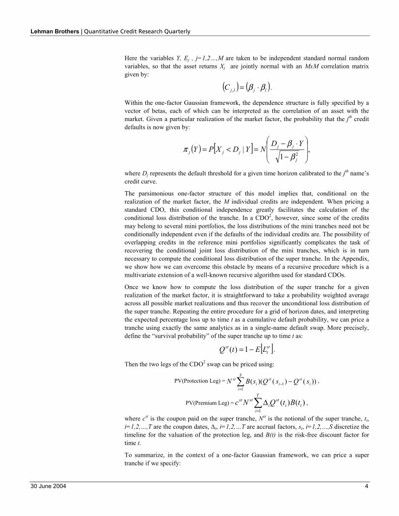
Figure 1 shows that this position offers an annual carry of about $256K. Under the modeling assumptions detailed above, a sudden default occurring immediately after the inception of the trade will cause a VOD loss of $356K, two defaults will cost the investor $672K and three defaults $940K. The position is also long correlation, with its mark-to-market gaining $53K if all betas increase by 1%. The positive systematic convexity of this position is captured in Figure 2, which shows that a generalized spread widening from 65bp to 100bp will produce a net gain of about $218,000. We stress that this is a stylized, albeit reasonably realistic trade, and that we are discussing model outputs without taking into account liquidity costs.

Figure 1. Carry, VOD, and Correlation Exposure of Delta-Hedged Equity Tranche

Annual Carry

($) VOD1

($) VOD2

($) VOD3

($)

Correlation Exposure(Net $ gain for 1% increase in betas)

Equity (0-5%) 256K 356K 672K 940K 53K

1 To compute VOD, one generally needs to specify not only the number but also the identities of the hypothesized

defaulters, since their deltas depend on name-specific inputs such as credit curves and betas. When dealing with an equally weighted homogeneous portfolio, however, it is sufficient to specify the number of hypothesized defaults.


30 June 2004 7

Figure 2. Systematic Convexity of Delta-Hedged Equity Tranche

0K

100K

200K

300K

400K

500K

600K

0 20 40 60 80 100 120 140

Spread

PV


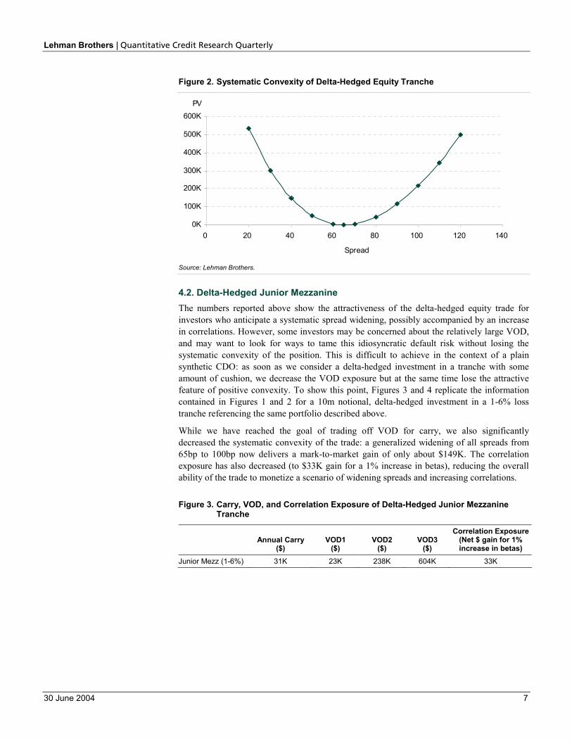
4.2. Delta-Hedged Junior Mezzanine The numbers reported above show the attractiveness of the delta-hedged equity trade for investors who anticipate a systematic spread widening, possibly accompanied by an increase in correlations. However, some investors may be concerned about the relatively large VOD, and may want to look for ways to tame this idiosyncratic default risk without losing the systematic convexity of the position. This is difficult to achieve in the context of a plain synthetic CDO: as soon as we consider a delta-hedged investment in a tranche with some amount of cushion, we decrease the VOD exposure but at the same time lose the attractive feature of positive convexity. To show this point, Figures 3 and 4 replicate the information contained in Figures 1 and 2 for a 10m notional, delta-hedged investment in a 1-6% loss tranche referencing the same portfolio described above.

While we have reached the goal of trading off VOD for carry, we also significantly decreased the systematic convexity of the trade: a generalized widening of all spreads from 65bp to 100bp now delivers a mark-to-market gain of only about $149K. The correlation exposure has also decreased (to $33K gain for a 1% increase in betas), reducing the overall ability of the trade to monetize a scenario of widening spreads and increasing correlations.

Figure 3. Carry, VOD, and Correlation Exposure of Delta-Hedged Junior Mezzanine Tranche

Annual Carry

($) VOD1

($) VOD2

($) VOD3

($)


Junior Mezz (1-6%) 31K 23K 238K 604K 33K


30 June 2004 8

Figure 4. Systematic Convexity of Delta-Hedged Junior Mezzanine Tranche

0K

50K

100K

150K

200K

250K

300K

350K

400K

0 20 40 60 80 100 120 140

Spread

PV


4.3. Delta-Hedged Super Equity A delta-hedged super equity tranche of a CDO2 referencing a portfolio of mezzanine tranches preserves a pronounced systematic convexity while efficiently trading off VOD for carry. To show this point, we first build three mini mezzanine tranches covering losses between 3% and 6%. Once again, each tranche references an equally weighted homogeneous portfolio of 100 names, each with a beta of 50%, a recovery rate of 40%, and a flat CDS curve of 65bp. The three reference portfolios overlap: each one has 40 unique names, 40 names that also belong to one of the other two portfolios, and 20 names that are common to all three portfolios.2

Next, we consider a 10MM notional, delta-hedged investment in a 0-5% super equity tranche referencing the three mini mezzanines described above. Figures 5 and 6 report the usual measures associated with this trade. First, notice that both the carry and the VOD profile of this trade are very close to those of the delta-hedged, 1-6% loss tranche analyzed above3. Most importantly, notice that this time the reduction of the idiosyncratic default risk did not come at the expense of either the correlation exposure or the systematic convexity. This “squared” delta-hedged equity investment has a positive correlation exposure of $54K for a 1% increase in betas, which is slightly higher than that of the delta-hedged 0-5% equity, and significantly higher than that of the delta-hedged 1-6% tranche. Moreover, figure 6 shows that a generalized increase in spreads from 65bp to 100bp now produces a net mark-to-market gain of approximately $261K.

Figure 5. Carry, VOD, and Correlation Exposure of Delta-Hedged Super Equity Tranche

Annual Carry

($) VOD1

($) VOD2

($) VOD3

($)


Super Equity (0-5%) of Three Mini Mezz (3-6%)

28K 11K 246K 726K 54K

2 This implies that the reference universe for the CDO2 consists of 200 issuers. 3 Since in our CDO2 the VOD numbers depend on whether the defaulter(s) belong(s) to one, two or all three of the

reference portfolios, we conservatively compute VOD assuming that each hypothesized defaulter belongs to all three mini portfolios.


30 June 2004 9

Figure 6. Systematic Convexity of Delta-Hedged Super Equity Tranche

0K

100K

200K

300K

400K

500K

600K

700K

0 20 40 60 80 100 120 140

Spread

PV


To help the reader summarize our findings, Figure 7 compares carry, VOD and correlation exposure for the three trades we have analyzed in this section, while Figure 8 compares their systematic convexities.

Figure 7. Carry, VOD, and Correlation Exposure of Three Delta-Hedged Loss Tranches

Annual Carry

($) VOD1

($) VOD2

($) VOD3

($)


Equity (0-5%) 256K 356K 672K 940K 53K Junior Mezz (1-6%) 31K 23K 238K 604K 33K Super Equity (0-5%) of Three Mini Mezz (3-6%)

28K 11K 246K 726K 54K

Figure 8. Systematic Convexity of Three Delta-Hedged Loss Tranches

0K

100K

200K

300K

400K

500K

600K

700K

0 20 40 60 80 100 120 140

Spread

PV

Equity Junior Mezz Super Equity



30 June 2004 10

APPENDIX: DERIVING THE LOSS DISTRIBUTION OF A SUPER TRANCHE

Our goal in this Appendix is to construct the cumulative loss distribution of a super tranche up to a given horizon. As mentioned in the main text, the possibility of overlapping credits in the reference mini portfolios significantly complicates the task of recovering the conditional joint loss distribution of the mini tranches, which is in turn necessary to compute the conditional loss distribution of the super tranche. To overcome this obstacle, we propose a recursive procedure which is a multivariate extension of a well-known recursive algorithm used for plain CDOs (see, for example, Greenberg et al (2004)).4

We first discretize losses in the event of default by associating each credit with the number of loss units that its default would produce in each of the mini portfolios: the representative element of the “loss matrix” ( )kj ,λ indicates the integer number of loss units in mini

portfolio k due to the default of name j.

Next, we construct an N-dimensional hyper-cube whose kth side consists of all possible loss levels for the kth mini portfolio, ie, ( )∑ =

M

j kj1 ,,...,1,0 λ . For ease of explanation, and without

loss of generality, we consider here a two-dimensional example (k=2). In this case, our hyper-cube is simply a matrix ( )

21 ,vvZ where we can store the conditional joint distribution

of the two mini portfolios; for example, we store in 5,3Z the probability of jointly having

three loss units in the first mini portfolio and five in the second. In order to obtain the correct set of joint probabilities, we first initiate each state (recursion step j=0) by setting:

,10, 21

=vvZ if 01 =v and 02 =v ,

00, 21

=vvZ otherwise.

Then, we feed the M credits, one at a time, through the following recursion:

( )( ) ( ) ( ) ( )1

,1

,, 2,21,121211 −

−−− ⋅+⋅−= j

vvjj

vvjj

vv jjZYZYZ λλππ if 2,21,1 jj vv λλ ≥∩≥

( )( ) 1,, 2121

1 −⋅−= jvvj

jvv ZYZ π otherwise,

where ( )Yjπ indicates the conditional probability that issuer j defaults. Each credit can

either survive, and every state then “keeps” its position, or default, in which case every state “moves” in the direction [λj,1, λj,2]. After including all the issuers, we set:

( ) ( )Mvvvv ZZ

2121 ,, = .

The matrix ( )21 ,vvZ now holds the joint loss distribution of the two mini portfolios

conditional on the realization of the market factor. It is then straightforward to recover the conditional joint distribution of losses on the mini tranches, the conditional loss distribution of the super portfolio and the conditional loss distribution of the super tranche. We can then proceed to integrate over the market factor, construct the tranche survival curve, and price the super tranche as described in the main text.

4 Greenberg, A., Mashal, R., Naldi, M., Schloegl, L. (2004), “Tuning Correlation and Tail Risk to the Market Prices of

Liquid Tranches”, Quantitative Credit Research, March 3-12.

The views expressed in this report accurately reflect the personal views of Prasun Baheti, Roy Mashal, Marco Naldi and Lutz Schloegl, theprimary analyst(s) responsible for this report, about the subject securities or issuers referred to herein, and no part of such analyst(s)’compensation was, is or will be directly or indirectly related to the specific recommendations or views expressed herein.

Any reports referenced herein published after 14 April 2003 have been certified in accordance with Regulation AC. To obtain copies of thesereports and their certifications, please contact Larry Pindyck ([email protected]; 212-526-6268) or Valerie Monchi ([email protected];44-(0)207-102-8035).

Lehman Brothers Inc. and any affiliate may have a position in the instruments or the Company discussed in this report. The Firm’s interestsmay conflict with the interests of an investor in those instruments.

The research analysts responsible for preparing this report receive compensation based upon various factors, including, among other things,the quality of their work, firm revenues, including trading, competitive factors and client feedback.

This material has been prepared and/or issued by Lehman Brothers Inc., member SIPC, and/or one of its affiliates (“Lehman Brothers”)and has been approved by Lehman Brothers International (Europe), authorised and regulated by the Financial Services Authority, inconnection with its distribution in the European Economic Area. This material is distributed in Japan by Lehman Brothers Japan Inc.,and in Hong Kong by Lehman Brothers Asia Limited. This material is distributed in Australia by Lehman Brothers Australia Pty Limited,and in Singapore by Lehman Brothers Inc., Singapore Branch. This material is distributed in Korea by Lehman Brothers International(Europe) Seoul Branch. This document is for information purposes only and it should not be regarded as an offer to sell or as asolicitation of an offer to buy the securities or other instruments mentioned in it. No part of this document may be reproduced in anymanner without the written permission of Lehman Brothers. We do not represent that this information, including any third party information,is accurate or complete and it should not be relied upon as such. It is provided with the understanding that Lehman Brothers is notacting in a fiduciary capacity. Opinions expressed herein reflect the opinion of Lehman Brothers and are subject to change withoutnotice. The products mentioned in this document may not be eligible for sale in some states or countries, and they may not be suitablefor all types of investors. If an investor has any doubts about product suitability, he should consult his Lehman Brothers representative.The value of and the income produced by products may fluctuate, so that an investor may get back less than he invested. Value andincome may be adversely affected by exchange rates, interest rates, or other factors. Past performance is not necessarily indicative offuture results. If a product is income producing, part of the capital invested may be used to pay that income. Lehman Brothers may, fromtime to time, perform investment banking or other services for, or solicit investment banking or other business from any companymentioned in this document. © 2004 Lehman Brothers. All rights reserved. Additional information is available on request. Please contacta Lehman Brothers’ entity in your home jurisdiction.

3. synthetic cdos of cdos - idc · lehman brothers | quantitative credit research quarterly 30 june...

Documents