3. review on transfer and processing of the continuous ... fileinternational journal of smart home...

International Journal of Smart Home

Vol.3, No.4, October, 2009

23

Review on Transfer and Processing of the Continuous Information

Minkyu Choi, Alisherov F.A, Seung-Hwan Jeon and Sattarova F.Y.

Hannam University, Daejeon, S.Korea [email protected]

Abstract

In this article some transport-layer access network deployment scenarios that show user equipment accessing the NGN are considered. The figures used to illustrate these cenarios show physical devices and indicate high-level functionality are shown. In the paper we are stating results of issue for developing: algorithms of analysis of quality and choice the most adequate activate function at neural network for smoothing of non-stationary process; algorithms of control the mistakes in the data of a non-stationary nature at formation of training subset; algorithms of adaptive training of neural networks in view of errors in structural components. The new technique and algorithm for analysis of information dynamic characteristics under their incremental characteristics, and also the general principles and rules for the adaptive control of data by non-stationary nature are developed. The general and private decisions of tasks, formulas for estimation of control optimum borders and of minimal mean square deviation are received for the control of the information at stationary, partial-stationary and non-stationary processes. Quality of Service is the subject of multiple researches in network technologies industry that’s why a group of scientists are always working out the new methods and algorithms, which provide corresponding quality of service. We will study this question from the position of routing protocols in on IP-based networks. An increasing number of emerging Internet applications require better than best effort quality of service (QoS) that is offered by the current Internet. Applications such as voice over IP, video on demand (VoD) need end-to-end QoS guarantees defined in terms of throughput, delay and loss rate. However, QoS guarantee for these services require to match optimal routing protocol. That is can significantly increase the complexity and affect the scalability of the network. This paper addresses the analysis of the backbone routing protocols. This paper focuses on relatively simple direct search methods for solving the optimization problem of minimizing a loss function L = Z (θ ) subject to the parameter vector 0 lying in some set 0. 1. Introduction This article describes some transport-layer access network deployment scenarios that show user equipment accessing the NGN. The figures used to illustrate these scenarios show physical devices and indicate highlevel functionality but do not indicate business models, enterprise roles, or operator domain boundaries. In general, many different business models may be used with each functional scenario. Some of the text used to describe the figures contains examples of such business model considerations. Also, note that the term "policy enforcement" as used here covers generalized transport-layer user-plane policy enforcement actions, such as QoS traffic conditioning, packet filtering, NAPT binding manipulation, usage metering, flow-based charging, and policy-based forwarding, which may in some cases be



24

broader in scope than NGN release 1. In this discussion, the terms "link layer" and "layer 2" are used synonymously. In the diagrams, some link-layer segments are shown with a specific type (e.g., VLAN (Virtual LAN)), but in general any type of link layer can be used (e.g., SDH (synchronous digital hierarchy), ATM, MPLS (multi protocol label switching)). As the convenient computer technology for adaptive processing of the data of non-stationary and poorly formalisable processes it is possible to note the use of the artificial neural networks (NN). At the same time, carrying out of researches for construction a neuronetworking information technology, allowing to intellectualize the specific processes of visualization, classifications, approximations and ordering of images of microobjects, fingerprints, elements of texts, schedules of technical and economic indicators for recognition and forecasting, where decisions of problems are brought to develop of methods and algorithms of processing of the information continuous by nature, is proved and is represents the big theoretical and practical interest. In article let’s state results of researches connected to development of methods and algorithms abetting to increase the quality of job of neuronetworking data processing systems (DPS) at the expense of identification error minimization during forming the NN’s training subsets and target parameters [1,2].

Table 1. Comparison of Link-State and Distance-Vector Routing Protocols.

Routers forward IP packets based on the destination IP address in the IP packet header. They compare the destination address to the routing table with the hope of finding a matching entry—an entry that tells the router where to forward the packet next. If the router does not match an entry in the routing table, and no default route exists, the router discards the packet. Therefore, having a full and accurate routing table is important. When first created distance vector protocols, routers had slow processors connected to slow links (relative to today’s technology). For perspective, RFC 1058, published as an Internet standard RFC in June 1988, defined the first version of RIP for IP. Therefore, distance vector protocols were designed to advertise just the basic routing information across the network to save bandwidth. Link-state



25

and balanced hybrid protocols were developed mainly in the early to mid 1990s, and they were designed under the assumptions of faster links and more processing power in the routers. By sending more information, and requiring the routers to perform more processing, these newer types of routing protocols can gain some important advantages over distance vector protocols—mainly, faster convergence. The goal remains the same—to add the currently-best routes to the routing table—but these protocols use different methods to find and add those routes.[3] Link-state routing protocols perform in a very different way from distance vector protocols. Understanding the difference between distance vector and link-state protocols is vital for network administrators. One essential difference is that distance vector protocols use a simpler method of exchanging routing information. Link-state routing protocols collect routing information from all other routers in the network or within a defined area of the network. Once all of the information is collected, each router, independently of the other routers, calculates its best paths to all destinations in the network. Because each router maintains its own view of the network, it is less likely to propagate incorrect information provided by any of its neighboring routers. In Table 1 you can see comparison between Link- State and Distance-Vector Routing Protocols. All distance vector protocols learn routes and then send these routes to directly connected neighbors. However, link-state routers advertise the states of their links to all other routers in the area so that each router can build a complete link-state database. These advertisements are called link-state advertisements (LSAs). Unlike distance vector routers, link-state routers can form special relationships with their neighbors and other linkstate routers. This is to ensure that the LSA information is properly and efficiently exchanged. The initial flood of LSAs provides routers with the information that they need to build a link-state database. Routing updates occur only when the network changes. If there are no changes, the routing updates occur after a specific interval. If the network changes, a partial update is sent immediately. The partial update only contains contains information about links that have changed, not a complete routing table. An administrator concerned about WAN link utilization will find these partial and infrequent updates an efficient alternative to distance vector routing, which sends out a complete routing table every 30 seconds. When a change occurs, link-state routers are all notified simultaneously by the partial update. Distance vector routers wait for neighbors to note the change, implement the change, and then pass it to the neighboring routers. The benefits of link-state routing over distance vector protocols include faster convergence and improved bandwidth utilization. Link-state protocols support classless interdomain routing (CIDR) and variable-length subnet mask (VLSM). This makes them a good choice for complex, scalable networks. In fact, link-state protocols generally outperform distance vector protocols on any size network. Link-state protocols are not implemented on every network because they require more memory and processing power than distance vector protocols and can overwhelm slower equipment. Another reason they are not more widely implemented is the fact that link-state protocols are quite complex. This would require well-trained administrators to correctly configure and maintain them. This paper examines several direct search methods for optimization, “direct” in the sense that the algorithms use minimal information about the loss function. These direct methods have the virtues of being simple to implement and having broad applicability. Further, it is sometimes possible to make rigorous statement about the convergence properties of the algorithms, which is not always possible in more complex procedures.



26

The information required to implement these methods is essentially only input-output data where θ is the input and Z (θ ) (noise-free) or y(θ ) (noisy) is the output. Further, the underlying assumptions about L are relatively minimal. In particular, there are no requirements that the gradient of L be computable (or even that the gradient exist) or that L be unimodal (i.e., that L have only one local optimum, corresponding to the global optimum). This paper focuses on two distinct types of popular direct search methods. The first is random search and the specialty is based on the geometric notion of a simplex. Note that when the random search or nonlinear simplex methods are applied to problems with differentiable L, these techniques make no use of the gradient that exists. Avoiding the use of the gradient can often significantly ease implementation. With the exception of some of the discussion on the nonlinear simplex method, the algorithms of this chapter have at least one of the two characteristics of stochastic search and optimization noisy input information or injected algorithm randomness. For purposes of algorithm evaluation by Monte Carlo, pseudorandom numbers generated via a computer algorithm are used to produce both the noise and the injected randomness. For purposes of actual application to a physical system producing its own randomness, pseudorandom numbers are used only for the injected randomness. There are never likely to be fully acceptable automated stopping criteria for stochastic search algorithms. For that reason, this paper will generally emphasize algorithm comparisons and stopping based on "budgets" of function evaluations. Nonetheless, sometimes one may wish to augment function budgets or analyst "intuition" via some automated approach. Two common stopping criteria are given below. Let r\ represent a small positive number, N be the number of iterations for which the algorithm should be "stable," and k θ be the estimate for θ at iteration k. An algorithm may be stopped at iteration n > N when, for all 1 <j < N, at

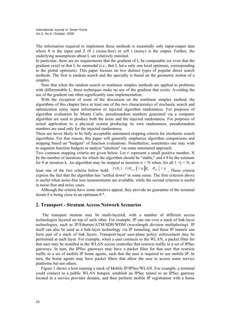
least one of the two criteria below hold: , These criteria express the fact that the algorithm has "settled down" in some sense. The first criterion above is useful when noise-free loss measurements are available, while the second criterion is useful in noise-free and noisy cases. Although the criteria have some intuitive appeal, they provide no guarantee of the terminal iterate θ n being close to an optimum θ *. 2. Transport - Stratum Access Network Scenarios The transport stratum may be multi-layered, with a number of different access technologies layered on top of each other. For example, IP can run over a stack of link-layer technologies, such as IP/Ethernet/ATM/SDH/WDM (wavelength division multiplexing). IP itself can also be used as a link-layer technology via IP tunneling, and these IP tunnels can form part of a stack of link layers. Transport-layer user-plane policy enforcement may be performed at each layer. For example, when a user connects to the WLAN, a packet filter for that user may be installed in the WLAN access controller that restricts traffic to a set of IPSec gateways. In turn, the IPSec gateways may have a packet filter for that user that restricts traffic to a set of mobile IP home agents, such that the user is required to run mobile IP. In turn, the home agents may have packet filters that allow the user to access some service platforms but not others. Figure 1 shows a host running a stack of Mobile IP/IPSec/WLAN. For example, a terminal could connect to a public WLAN hotspot, establish an IPSec tunnel to an IPSec gateway located in a service provider domain, and then perform mobile IP registration with a home



27

agent also in the service provider domain. In this example, a co-located care-of address is used, so there is no foreign agent. Here, the terminal has three IP addresses, one for each layer. The first IP address is assigned when the terminal connects to the WLAN network; the second, when the terminal connects to the IPSec gateway; and the third, when mobile IP registration is performed. Also, an AAA request may be issued independently at each layer for the purposes of user authentication and authorization. The terminal may send all application traffic over mobile IP, or it can bypass one or more layers in the stack and send application traffic via a lower layer. For example, split IPSec tunneling could be used, whereby only traffic destined to the service provider domain is sent via IPSec, with general Internet traffic bypassing IPSec.

Figure 1. Multi-layered transport stratum

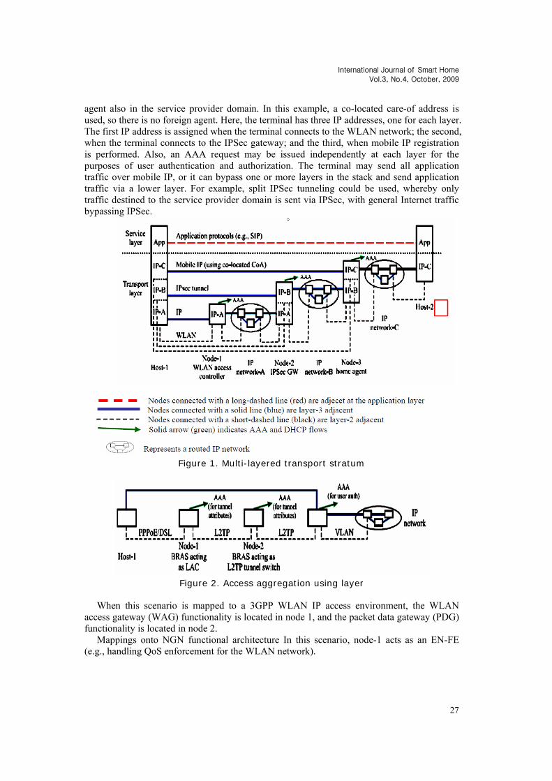
Figure 2. Access aggregation using layer

When this scenario is mapped to a 3GPP WLAN IP access environment, the WLAN access gateway (WAG) functionality is located in node 1, and the packet data gateway (PDG) functionality is located in node 2. Mappings onto NGN functional architecture In this scenario, node-1 acts as an EN-FE (e.g., handling QoS enforcement for the WLAN network).



28

Node-1 may also act as an ABG-FE (e.g., performing NAPT). Node-2 and node-3 act as ABG-FEs, handling policy enforcement for their respective IP layers. This scenario illustrates that ABG-FE and EN-FE functionality may be performed independently at each IP layer in a transport stratum which contains multiple IP layers. Node-2 and node-3 may also act as EN-FEs, handling QoS enforcement for the IP tunnels for which they are performing a layer-2 termination function. This scenario illustrates that ABG-FE and EN-FE functionality may be performed independently at each IP layer in a transport stratum which contains multiple IP layers. Within a single layer of the transport stratum, there may be multiple points where access traffic is aggregated. Traffic forwarding between different aggregation segments may be done at layer 2 or layer 3. Figure II.2 shows a host running PPPoE connected over DSL (digital subscriber line) to a BRAS (broadband remote access server). This BRAS acts as a LAC (L2TP access concentrator) and forwards the traffic by using L2TP to a second BRAS acting as an LNS (L2TP network server). Node 1 may issue a RADIUS request to obtain attributes for the tunnel to be established (e.g., RFC 2868). The second BRAS performs L2TP tunnel switching and in turn acts as a LAC and forwards the traffic to a third BRAS acting as an LNS. Node 2 may also issue a RADIUS request to obtain attributes for the tunnel to be established. The third BRAS terminates the PPP state machine and may issue a RADIUS request to perform user authentication. Forwarding at nodes 1 and 2 is done at layer 2, with traffic being switched between two link-layer segments: IP header information is not examined in making forwarding decisions. Policy enforcement (e.g., traffic conditioning, packet filtering, NAPT, etc.) is generally only done in node 3, though there are cases where some policy enforcement may be done at nodes 1 or 2. For example, a similar scenario can be used in a mobile environment with a mobile operator providing a network-based VPN service and backhauling traffic to a corporate LNS. If a pre-paid charging model is used, service termination upon reaching a zero-balance condition may be enforced at nodes 1 or 2. The scenario shown here may be used in a wholesale business model, where one party owns the physical DSL lines and aggregates traffic to a second party acting as a wholesaler, who in turn aggregates traffic to a third party acting as a service provider (e.g., an ISP). By introducing a wholesale intermediary, the party dealing with the physical lines (or more generally, the party operating the access-technology-specific equipment) does not need to maintain a business relationship with all the service providers, and a party acting as a service provider does not need to maintain a business relationship with multiple operators each handling some specific access technology, such as DSL, 2G/3G, or WiMax (worldwide interoperability for microwave access). 2.1.Mappings onto NGN functional architecture In this scenario, node-1 acts as an EN-FE (e.g., handling QoS enforcement for the DSL aggregation network). Node-3 acts an ABG-FE (e.g., performing traffic conditioning, packet filtering, NAPT, etc.). Node-3 may also act as an EN-FE, handling QoS enforcement for the L2TP tunnels it terminates. Typically node-2 is acting as a pure layer-2 relay and is not playing either an EN-FE or an ABG-FE role. Node-2 acts as an ABGFE if it is performing IP-level policy enforcement (e.g., accounting).



29

Figure 3. Access aggregation using layer 3 This is similar to Figure 2, except that forwarding between different aggregation segments is done at layer 3. Node 1 terminates PPP and associates the traffic for a PPP session with a particular domain (e.g., using the realm part of the PPP username to identify the domain). In the upstream direction, policy-based forwarding is used, so that traffic for different domains is segregated and the correct IP next-hop for each domain is chosen. In the downstream direction, node 1 performs regular IP forwarding based on the longest match prefix. Node 2 implements multiple virtual routers, one for each domain. Again, policy-based forwarding is done in the upstream direction, such that all traffic for a given user is sent upstream to node 3, and regular IP forwarding is done in the downstream direction. In this example, nodes 1, 2, and 3 see all the traffic for a given subscriber. Node 1 may issue a RADIUS request to perform user authentication. This request may be sent via a RADIUS proxy, or directly over the virtual routed network itself, thus avoiding the need for a RADIUS proxy. Aggregation at layer 3 may simplify node 3, since it does not need to terminate large numbers of L2TP tunnels and associated PPP state machines, but it instead receives an aggregated traffic stream delivered over a single VLAN. Note that node 3 can still identify individual subscriber traffic flows for the purposes of performing subscriber-specific policy enforcement actions, but on the user plane this is done using layer-3 information (e.g., the source IP address) rather than by maintaining an individual link-layer connection for Transport - each subscriber. Policy enforcement actions (e.g., traffic conditioning, packet filtering, NAPT, etc.) may be carried out in all nodes, and this may be done at the subscriber-flow level or at coarser granularities such as at the virtual router level (e.g., some VRs may have a higher level of QoS than others). Mappings onto NGN functional architecture In this scenario, node-1 acts as an EN-FE (e.g., handling QoS enforcement for the DSL aggregation network). Node-3 acts an ABG-FE (e.g., performing traffic conditioning, packet filtering, NAPT, etc.). Node-1 and node-2 act as ABG-FEs if they are performing IP-level policy enforcement (e.g., NAPT or support of different QoS classes). Node-2 and node-3 may also act as EN-FEs, handling QoS enforcement for the VLANs they terminate.

Figure 4. Multi-stage policy enforcement

Within a single layer of the transport stratum, the set of policy enforcement actions carried out for traffic for a given subscriber may be distributed across a sequence of devices, with each device doing a subset of the total work. This may reflect a network deployment strategy



30

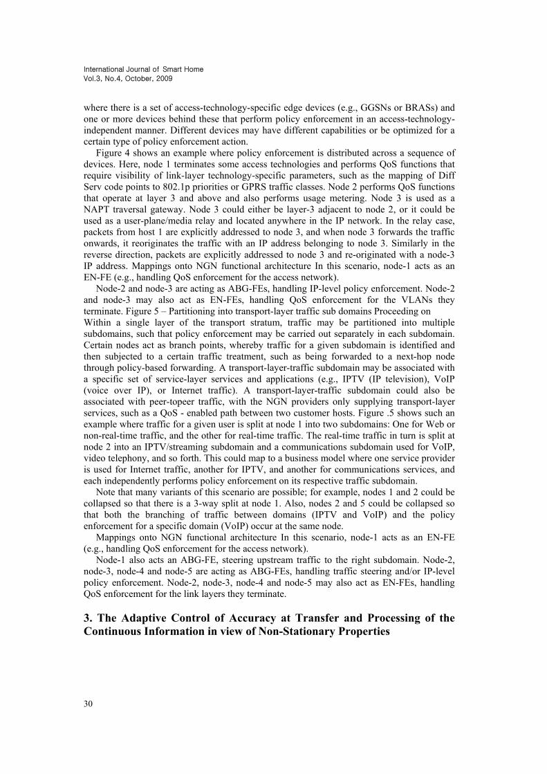
where there is a set of access-technology-specific edge devices (e.g., GGSNs or BRASs) and one or more devices behind these that perform policy enforcement in an access-technology-independent manner. Different devices may have different capabilities or be optimized for a certain type of policy enforcement action. Figure 4 shows an example where policy enforcement is distributed across a sequence of devices. Here, node 1 terminates some access technologies and performs QoS functions that require visibility of link-layer technology-specific parameters, such as the mapping of Diff Serv code points to 802.1p priorities or GPRS traffic classes. Node 2 performs QoS functions that operate at layer 3 and above and also performs usage metering. Node 3 is used as a NAPT traversal gateway. Node 3 could either be layer-3 adjacent to node 2, or it could be used as a user-plane/media relay and located anywhere in the IP network. In the relay case, packets from host 1 are explicitly addressed to node 3, and when node 3 forwards the traffic onwards, it reoriginates the traffic with an IP address belonging to node 3. Similarly in the reverse direction, packets are explicitly addressed to node 3 and re-originated with a node-3 IP address. Mappings onto NGN functional architecture In this scenario, node-1 acts as an EN-FE (e.g., handling QoS enforcement for the access network). Node-2 and node-3 are acting as ABG-FEs, handling IP-level policy enforcement. Node-2 and node-3 may also act as EN-FEs, handling QoS enforcement for the VLANs they terminate. Figure 5 – Partitioning into transport-layer traffic sub domains Proceeding on Within a single layer of the transport stratum, traffic may be partitioned into multiple subdomains, such that policy enforcement may be carried out separately in each subdomain. Certain nodes act as branch points, whereby traffic for a given subdomain is identified and then subjected to a certain traffic treatment, such as being forwarded to a next-hop node through policy-based forwarding. A transport-layer-traffic subdomain may be associated with a specific set of service-layer services and applications (e.g., IPTV (IP television), VoIP (voice over IP), or Internet traffic). A transport-layer-traffic subdomain could also be associated with peer-topeer traffic, with the NGN providers only supplying transport-layer services, such as a QoS - enabled path between two customer hosts. Figure .5 shows such an example where traffic for a given user is split at node 1 into two subdomains: One for Web or non-real-time traffic, and the other for real-time traffic. The real-time traffic in turn is split at node 2 into an IPTV/streaming subdomain and a communications subdomain used for VoIP, video telephony, and so forth. This could map to a business model where one service provider is used for Internet traffic, another for IPTV, and another for communications services, and each independently performs policy enforcement on its respective traffic subdomain. Note that many variants of this scenario are possible; for example, nodes 1 and 2 could be collapsed so that there is a 3-way split at node 1. Also, nodes 2 and 5 could be collapsed so that both the branching of traffic between domains (IPTV and VoIP) and the policy enforcement for a specific domain (VoIP) occur at the same node. Mappings onto NGN functional architecture In this scenario, node-1 acts as an EN-FE (e.g., handling QoS enforcement for the access network). Node-1 also acts an ABG-FE, steering upstream traffic to the right subdomain. Node-2, node-3, node-4 and node-5 are acting as ABG-FEs, handling traffic steering and/or IP-level policy enforcement. Node-2, node-3, node-4 and node-5 may also act as EN-FEs, handling QoS enforcement for the link layers they terminate. 3. The Adaptive Control of Accuracy at Transfer and Processing of the Continuous Information in view of Non-Stationary Properties



31

The computer systems of transfer and processing information, in particular, systems of teleprocessing given results of physical, chemical, biological researches, the automated control systems of technological processes, of stand tests and other systems of telemeasurement form the large volume of continuous on a nature information. The messages transmitted and processable in these systems, are exposed to distortions, and, the basic sources of mistakes are: influence of handicapes in channels of communication; failures and refusals of information processing means and control facilities; mistakes connected to job of the operator. It is necessary to note, that now basic methods of researches are directed on increase of a degree of information reliability on channels outputs and outputs of means used for transfer, formation and processing of the information. It is accumulated the wide experience of application of organizational, code and hardware methods wich have aim of detection and correction of mistakes allowing to ensure required level of information transfer reliability. As theoretical rules of quality estimation for reliable information transfer in thus serves the researches for reception the quantitative characteristics of the information, basically, on probabilistic criteria, in particular, on criteria of detected and non-detected mistakes probabilities or on criteria of information correct reception probability, in which questions of mistakes detection in the data are mainly [3-5]. Alongside with it, at processing the information, the research and mathematical substantiation of reception the estimations of information control quality for correction mistakes in the data represent large interest. It is necessary to note, that on a basis of apriory items about statistical characteristics of information continuous on a nature we can construct the methods, models, algorithms of increase of information control accuracy by known statistical criteria, for example, criteria Pirson’s, Kolmogorov’s criterias, rule of three sigmas, and also the methods of a dot or interval estimation, Bayeses decision, borders of the solved values etc. These traditional ways of the information control are widely applied in practice of management of organizing technical systems and technological processes. Other methodical basis of the information control accuracy is formed also by methods used at diagnosing of reliability industrial equipment, the receptions of the control and tracking job of information systems of technological parameters measurement etc. As important tool of construction the methods of the control accuracy for the information on a continuous nature serve results of development under the adaptive control of the information reliability at transfer and processing on the basis of natural redundancy [7]. 3.1 Control of the Data Accuracy for Nn Realization of researches for increase of quality of the continuous on a nature information control by mistakes correction requires construction the new researche plan of information accuracy control by qualitative criteria, in particular, criteria of minimal mean-square error is very convenient and effective. The works [8-10] of author also confirm, that use the criteria of minimal mean-square error of control the transmitted and processable data creates additional conditions and allows to develop adaptive methods and algorithms both for increase of training subsets forming quality, and for control of neuronetworking DPS target parameters errors at the expense of account statistical and dynamic characteristics of the visual information. In this connection, let’s show results of development the methods and adaptive algorithms of control and reduction error of NN’s training subset and target parameters on the basis of account statistical and dynamic characteristics of the information which non-stationary by nature.



32

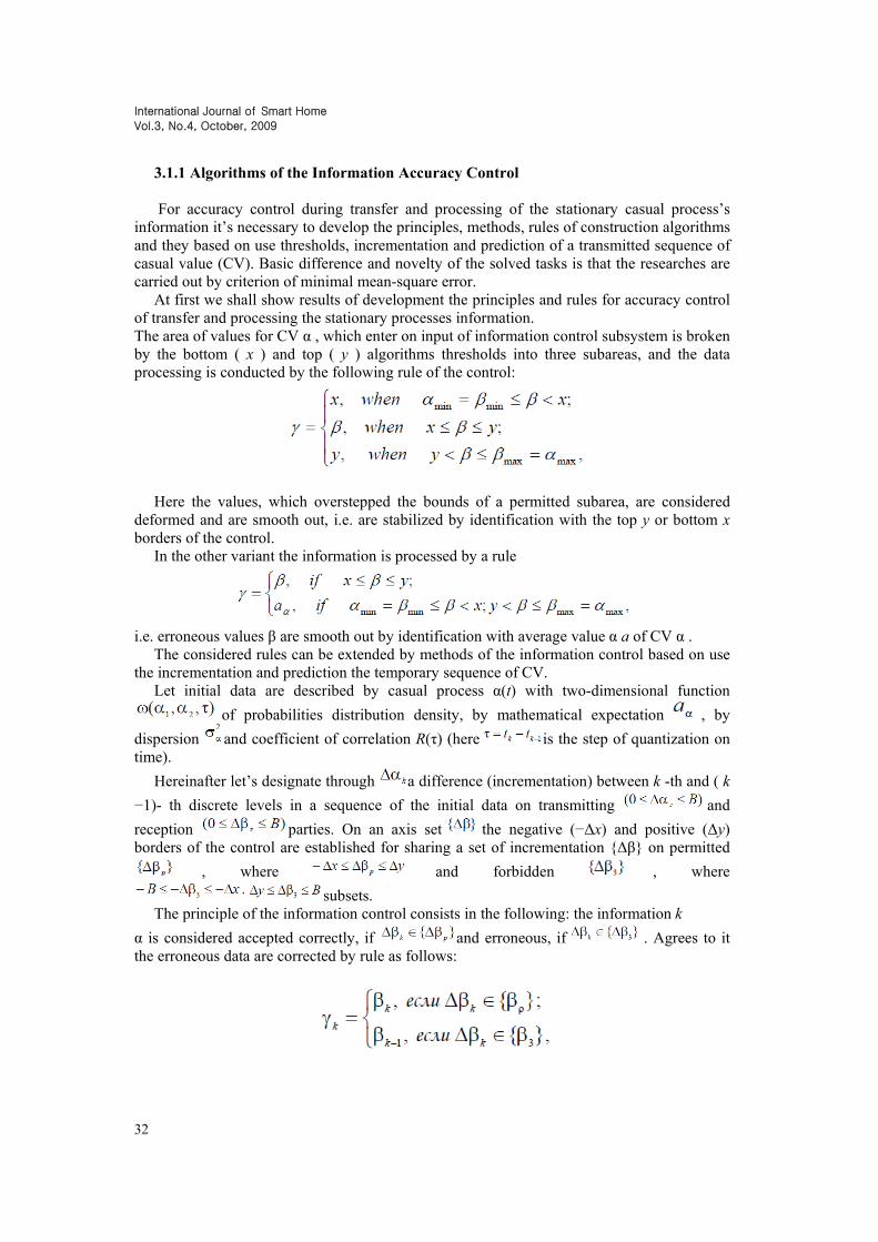
3.1.1 Algorithms of the Information Accuracy Control For accuracy control during transfer and processing of the stationary casual process’s information it’s necessary to develop the principles, methods, rules of construction algorithms and they based on use thresholds, incrementation and prediction of a transmitted sequence of casual value (CV). Basic difference and novelty of the solved tasks is that the researches are carried out by criterion of minimal mean-square error. At first we shall show results of development the principles and rules for accuracy control of transfer and processing the stationary processes information. The area of values for СV α , which enter on input of information control subsystem is broken by the bottom ( x ) and top ( y ) algorithms thresholds into three subareas, and the data processing is conducted by the following rule of the control:

Here the values, which overstepped the bounds of a permitted subarea, are considered deformed and are smooth out, i.e. are stabilized by identification with the top y or bottom x borders of the control. In the other variant the information is processed by a rule

i.e. erroneous values β are smooth out by identification with average value α a of СV α . The considered rules can be extended by methods of the information control based on use the incrementation and prediction the temporary sequence of СV. Let initial data are described by casual process α(t) with two-dimensional function

of probabilities distribution density, by mathematical expectation , by

dispersion and coefficient of correlation R(τ) (here is the step of quantization on time).

Hereinafter let’s designate through a difference (incrementation) between k -th and ( k

−1)- th discrete levels in a sequence of the initial data on transmitting and

reception parties. On an axis set the negative (−Δx) and positive (Δy) borders of the control are established for sharing a set of incrementation {Δβ} on permitted

, where and forbidden , where

subsets. The principle of the information control consists in the following: the information k

α is considered accepted correctly, if and erroneous, if . Agrees to it the erroneous data are corrected by rule as follows:



33

where k γ is value of CV k α , processed on the reception party. It means that the erroneous

information smoothes out by an identification with the previous value of initial process. The rules of the information control with a prediction of stationary process perform the

check of a difference between the transferred and predicted value of instead of

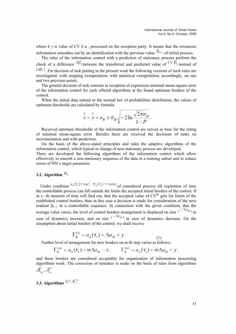
. For decision of task putting in the present work the following versions of such rules are investigated: with stepping extrapolation; with statistical extrapolation, accordingly, on one and two previous points. The general decision of task consists in reception of expression minimal mean-square error of the information control for each offered algorithms at the found optimum borders of the control. When the initial data submit to the normal law of probabilities distribution, the values of optimum thresholds are calculated by formula

Received optimum thresholds of the information control are served as base for the rating of minimal mean-square error. Besides there are received the decisions of tasks on incrementation and with prediction. On the basis of the above-stated principles and rules the adaptive algorithms of the information control, which typical to change of non-stationary process are developed. There are developed the following algorithms of the information control which allow effectively to smooth a non-stationary sequence of the data in a training subset and to reduce errors of NN’s target parameter.

3.2. Algorithm

Under condition of considered process till expiration of time the controllable process can fall outside the limits the accepted initial borders of the control. If in tk -th moment of time will find out, that the accepted value of СVβk gets for limits of the established control borders, then in this case a decision is made for consideration of the next readout βk+1 in a controllable sequence. In connection with the given condition, that the

average value varies, the level of control borders arrangement is displaced on size in

case of dynamics increase, and on size in case of dynamics decrease. On the assumption about initial borders of the control, we shall receive

(1) Further level of arrangement for new borders on m-th step varies as follows:

and these borders are considered acceptable for organization of information processing algorithms work. The correction of mistakes is made on the basis of rules from algorithms

3.3. Algorithms



34

Under condition of considered process there is defined as the significant minimal difference of mean-square rejections between various statuses of

process for the supervision period . In case of exit these readout from limits of the control borders we consider, that the information is accepted correctly, however their values fall outside the limits of control borders at the expense of change the controllable processes dynamics. Two variants of expansion of the control borders are considered.

Algorithm , where it is taken into account growth of controllable processes dynamics and

the top border extends on size , i.e. . Algorithm , where it is taken into account decrease of controllable processes dynamics and the bottom

border extends on size , i.е. the control of information for n-th step will be carried out

on borders .

3.4. Аlgorithm

Under condition the algorithm takes into account changes of

average value and mean-square rejection of controllable process and parameters are

set for the supervision period The adaptation of arrangement level and borders width for the control continue before hit of processes trajectory in limits of the control borders.

where through 1 n is designated a step of adaptation for top border, and through 2 n is designated a step for bottom border of the control algorithm. For adaptive algorithms of the control of information with non-stationary nature there is received the general expression of errors extreme value rating. The results are received for Laugranges and Newtons polynomials, R.Brauns adaptive model, models of neural network at exponential, bell-figurative and triangular functions of autocorrelation. 4. Analysis of the backbone routing protocols 4.1. Enhanced Interior Gateway Routing Protocol EIGRP operates quite differently from IGRP. EIGRP is an advanced distance vector routing protocol and acts as a link-state protocol when updating neighbors and maintaining routing information. The advantages of EIGRP over simple distance vector protocols include the following: � Rapid convergence � Efficient use of bandwidth



35

� Support for variable-length subnet mask (VLSM) and classless interdomain routing (CIDR). Unlike IGRP, EIGRP offers full support for classless IP by exchanging subnet masks in routing updates. � Multiple network-layer support � Independence from routed protocols. Protocol-dependent modules (PDMs) protect EIGRP from lengthy revision. Evolving routed protocols, such as IP, may require a new protocol module but not necessarily a reworking of EIGRP. EIGRP routers converge quickly because they rely on DUAL. DUAL guarantees loop-free operation at every instant throughout a route computation allowing all routers involved in a topology change to synchronize at the same time. EIGRP makes efficient use of bandwidth by sending partial, bounded updates and its minimal consumption of bandwidth when the network is stable. EIGRP routers make partial, incremental updates rather than sending their complete tables. This is similar to OSPF operation, but unlike OSPF routers, EIGRP routers send these partial updates only to the routers that need the information, not to all routers in an area. For this reason, they are called bounded updates. Instead of using timed routing updates, EIGRP routers keep in touch with each other using small hello packets. Though exchanged regularly, hello packets do not use up a significant amount of bandwidth. EIGRP supports IP, IPX, and AppleTalk through protocol-dependent modules (PDMs). EIGRP can redistribute IPX RIP and SAP information to improve overall performance. In effect, EIGRP can take over for these two protocols. An EIGRP router will receive routing and service updates, updating other routers only when changes in the SAP or routing tables occur. Routing updates occur as they would in any EIGRP network, using partial updates. EIGRP can also take over for the AppleTalk Routing Table Maintenance Protocol (RTMP). As a distance vector routing protocol, RTMP relies on periodic and complete exchanges of routing information. To reduce overhead, EIGRP redistributes AppleTalk routing information using event-driven updates. EIGRP also uses a configurable composite metric to determine the best route to an AppleTalk network. RTMP uses hop count, which can result in suboptimal routing. AppleTalk clients expect RTMP information from local routers, so EIGRP for AppleTalk should be run only on a clientless network, such as a wide-area network (WAN) link.

Figure 5. EIGRP working algorithm. Legend: Protocol Type — EIGRP, FD —

Feasible Distance, RD — Reported Distance as advertised by neighbor router,



36

Successor — Primary Route to Destination, FS — Feasible Successor - Backup route to Destination.

4.2 Simulated parameters comparison Imitation model which we simulated devoted to the IP-backbone with taking into account QoS main parameters and choosing the fastest routing protocol will be built. Below we presented results of imitation model of simulated IP backbone network, where shown comparison between four types of routing protocols, which are EIGRP, IGRP, OSPF and RIP:

Figure 6. Simulated parameters comparison. Video Conferencing packets end-to-end delay and Video Conferencing packets delay variation in different backbone

routing protocols

Figure 7. Simulated parameters comparison. IP Network Convergence Activity in different backbone routing protocols.



37

5. Direct search methods to solve stochastic optimization problem Random search methods for optimization are based on exploring the domain θ in a random manner to find a point that minimizes L = Z (θ ) . These are the simplest methods of stochastic optimization and can be quite effective in some problems. Their relative simplicity is an appealing feature to both practitioners and theoreticians. These direct random search methods have all or some of the following advantages relative to most other search methods. Some of these attributes were mentioned in the prescient paper of Karnopp (1963): (i) Ease of programming. The methods described below are relatively easy to code in software and can thereby significantly reduce the human cost of an optimization process (not to be ignored in practice, but often ignored in published results comparing the efficiency of one algorithm against another!). (ii) Use of only L measurements. The reliance on L measurements alone can significantly reduce the incentive to pick a loss function largely for analytical convenience—perhaps at a sacrifice to the true optimization goals—so that gradients or other ancillary information may be computed. Karnopp (1963) aptly calls this a reduction in "artful contrivance." (iii) Reasonable computational efficiency. Although not generally the most computationally efficient algorithms in practical problems, the algorithms can often provide reasonable solutions fairly quickly, especially if the problem dimension p (= dim(θ )) is not too large. This is especially true in those direct search algorithms that make use of some local information in their search (e.g., random search algorithms B and C below). For example, as demonstrated in Anderssen and Bloomfield (1975), random search may be more efficient than corresponding deterministic algorithms based on searches over multidimensional grids when p is large. The solution from a random search method can usually be augmented with some more powerful—but perhaps more complex— search algorithm if a more accurate solution is required. In fact, the random search algorithms may provide a means of finding "good" initial conditions for some of the more sophisticated algorithms to be presented later. For example, as demonstrated in Anderssen and Bloomfield (1975), random search may be more efficient than corresponding deterministic algorithms based on searches over multidimensional grids when p is large. The solution from a random search method can usually be augmented with some more powerful—but perhaps more complex—search algorithm if a more accurate solution is required. In fact, the random search algorithms may provide a means of finding "good" initial conditions for some of the more sophisticated algorithms to be presented later. (iv) Generality. The algorithms can apply to virtually any function. The user simply needs to specify the nature of the sampling randomness to allow an adequate search in θ . Thus, if θ is continuous valued, the sampling distribution should be continuous (e.g., Gaussian or continuously uniform on θ ); likewise, a discrete-valued θ calls for a discrete sampling distribution with nonzero probability of hitting the candidate points and a hybrid θ calls for the appropriate mix of continuous and discrete sampling distributions. (v) Theoretical foundation. Unlike some algorithms, supporting theory is often available to provide guarantees of performance and guidance on the expected accuracy of the solution. In fact, the theory may even be exact in finite samples, which is virtually unheard of in the analysis of other stochastic algorithms. 5.1 Three Algorithms for Random Search



38

Beginning with the most basic algorithm, this subsection describes three direct random search techniques. Because direct random search is a large subject unto itself, only a small selection of algorithms is being presented here in order to keep this subsection of manageable length. The three algorithms here are intended to convey the essential flavor of most available direct random search algorithms. The methods of this subsection assume perfect (noise-free) values of L. In the noise-free case, it can be shown that many random search methods converge to an optimum θ * in one of the probabilistic senses – almost surely (a.s.), in probability (pr.), or in mean square (m.s.)— as the number of L evaluations gets large. Realistically, however, these convergence results may have limited utility in practice since the algorithms may take a prohibitively large number of function evaluations to reach a value close to θ *, especially if p is large. This is illustrated below. Nevertheless, the formal convergence provides a guarantee not always available in other approaches. The simplest random search method is one where we repeatedly sample over θ such that the current sampling for θ does not take into account the previous samples. This "blind search" approach does not adapt the current sampling strategy to information that has been garnered in the search up to the present time. The approach can be implemented in batch (nonrecursive) form simply by laying down a number of points in θ and taking the value of θ yielding the lowest Z value as our estimate of the optimum. The approach can also be implemented in recursive form as we illustrate below. The simplest setting for conducting the random sampling of new (candidate) values of θ is when θ is a hypercube (a p-fold Cartesian product of intervals on the real line) and we are using uniformly generated values of θ . The uniform distribution is continuous or discrete for the elements of θ depending on the definitions for these elements. In fact, this particular (blind search) form of the algorithm is unique among all general stochastic search and optimization algorithms in this book: It is the only one without any adjustable algorithm coefficients that need to be "tuned" to the problem at hand. For a domain θ that is not a hypercube or for other sampling distributions, one may use transformations, rejection methods, or Markov chain Monte Carlo to generate the sample θ values. For example, if θ is an irregular shape, one can generate a sample on a hypercube superset containing θ and then reject the sample point if it lies outside of θ. A recursive implementation of the simple random search idea is as follows. This algorithm, called algorithm A here, applies when θ has continuous, discrete, or hybrid elements. 5.1.1 Algorithm A: Simple Random ("Blind") Search Step 0. (Initialization) Choose an initial value of Ө, say θ0 € Ө, either randomly or deterministically. (If random, usually a uniform distribution on Ө is used.) Calculate L ( ) θ0• Set k = 0.

Step 1. Generate a new independent value , according to the chosen probability distribution.

If . Step 2. Stop if the maximum number of L evaluations has been reached or the user is otherwise satisfied with the current estimate for θ via appropriate stopping criteria; else, return to step 1 with the new k set to the former k + 1. Algorithm A is the simplest random search in that the sampling generating the new θ value at each iteration is over the entire domain of interest. The sampling does not take account of where the previous estimates of θ have been. The two algorithms below, although still simple, are slightly more sophisticated in that the random sampling is a function of the position of the current best estimate for θ. In this way,



39

the search is more localized in the neighborhood of that estimate, allowing for a better exploitation of information that has previously been obtained about the shape of the loss function. Such algorithms are sometimes referred to as localized algorithms to emphasize their dependence on the local environment near the current estimate for 0. This terminology is not to be confused with the global versus local algorithms discussed in Chapter 1, where the emphasis is on searching for a global or local solution to the optimization problem. In fact, sometimes a localized algorithm is guaranteed to provide a global solution, as discussed below following the presentation of the first localized algorithm. Algorithm B is the first of the two localized algorithms we consider. This algorithm was described in Matyas (1965) and Jang et al. (1997). 5.1.2 Algorithm B: Localized Random Search Step 0 (Initialization) Pick an initial guess θ0 € Ө, either randomly or with prior information. Set k = 0.

Step 1 Generate an independent random vector and add it to the current θ value,

θ k . Check if , generate a new dë and repeat or, alternatively,

move to the nearest valid point within Ө. Let Өnew (k+l) equal θk + dk € Ө or the aforementioned nearest valid point in Ө. Step 2 If L(Өnew(k + 1)) < L(Ө k ), set (k+1) θ = (k +1) new θ ; else, set 1 + k θ = k θ . Step 3 Stop if the maximum number of L evaluations has been reached or the user is otherwise satisfied with the current estimate for 9 via appropriate stopping criteria; else, return to step 1 with the new k set to the former k + 1. Although Matyas (1965) and others have used the (multivariate) normal distribution for generating d k , the user is free to set the distribution of the deviation vector d k . The distribution should have mean zero and each component should have a variation (e.g., standard deviation) consistent with the magnitudes of the corresponding Ө elements. So, for example, if the magnitude of the first component in Ө lies between θ and 0.05 while the magnitude of the second component is between θ and 500, the corresponding standard deviations in the components of d ë might also vary by a magnitude of 10,000). This allows the algorithm to assign roughly equal weight to each of the components of Ө as it moves through the search space. Although not formally allowed in the convergence theorem below, it is often advantageous in practice if the variability in d ë is reduced as k increases. This allows one to focus the search more tightly as evidence is accrued on the location of the solution (as expressed by the location of our current estimate Ө k ). A simple implementation of this idea would be to reduce the variances by a factor such as k when the normal distribution is used in generating the d k . For the numerical studies below, we use the simple (constant variance) sampling, d k ~ N(0, p 2 Ip) for all k where p 2 represents the (common) variance of each of the components in d k . The convergence theory for the localized algorithms tends to be more restrictive than the theory for algorithm A. Solis and Wets (1981) provide a theorem for global convergence of localized algorithms, but the theorem conditions may not be verifiable in many practical applications. Their theorem would, in principle, cover both algorithm B and the enhanced algorithm C below. Other results related to formal convergence to global optima of various localized random search algorithms appear, for example, in Yakowitz and Fisher (1973) and Zhigljavsky (1991). An earlier theorem from Matyas (1965) (with proof corrected



40

in Baba et al., 1977) provides for global convergence of algorithm B if Z is a continuous function. The convergence is in the "in probability" (pr.) sense. Algorithm B above might be considered the most naive of the localized random search algorithms. More sophisticated approaches are also easy to implement. For instance, if a search in one direction increases Z, then it is likely to be beneficial to move in the opposite direction. Further, successive iterations in a direction that tend to consistently reduce Z should encourage further iterations in the same direction. Many algorithms exploiting these simple properties exist (e.g., Solis and Wets, 1981; Zhigljavsky, 1991; Li and Rhinehart, 1998; and the nonlinear simplex algorithm). An extensive survey emphasizing such algorithms developed prior to 1980 is given in Schwefel (1995). An example algorithm is given below (from Jang et al., 1997), which is a slight simplification of an algorithm in Solis and Wets (1981). The full Solis and Wets algorithm includes an even greater degree of adaptivity to the current environment, but this comes at the expense of more complex implementation. 5.1.3 Algorithm C: Enhanced Localized Random Search Step 0. (Initialization) Pick an initial guess θ0 € Ө, either randomly or with prior information. Set k = 0. Set bias vector b 0 = 0. Step 1. Generate an independent random vector dk and add it and the θ bias term bk to the

current value θk. Check if , generate a new d k and repeat;

alternatively, move to the nearest valid point within Ө. Let equal

or the above-mentioned nearest valid point in Ө.

Step 2. If go to step 5. Otherwise, go to step 3.

Step 3. Analogous to step 1, let or its altered version within Ө. If Ө (Ө'new(k +1)) < L(θk), set θ1 + k = θ 'new(k + 1) and bk+1 = bk - 0,4dk ; go to step 5 2 . Otherwise, go to step 4.

Step 4. Set - Go to step 5. Step 5. Stop if the maximum number of L evaluations has been reached or the user is otherwise satisfied with the current estimate for Ө via appropriate stopping criteria; else, return to step 1 with the new k set to the former k+l. Example.—Random search algorithms applied to Rosenbrock function. Consider the well-known Rosenbrock test function in the optimization literature. This test function was first presented in Rosenbrock (1960) for the p = 2 setting, with higher-dimensional extensions given in, among other places. This test function has an interesting shape in that the solution lies in a curved valley when considered in two-dimensional space. For general p, the function has the fourth-order polynomial form

where and p is divisible by 2.

Let us consider a problem where p = 10. Note that . Let the

constraint set be the Cartesian product of intervals . Table 2.5 presents the results of the study based on 40 independent runs for each algorithm. Each run of algorithms A and B uses 1000 loss evaluations; algorithm C is terminated at the 1000th loss evaluation or the first possible loss after the 1000th (it is not possible to specify a priori the exact number of



41

measurements needed by algorithm C). Each run was started at the initial condition

= 121; this is a common initial condition in numerical studies with this function). The confidence intervals are computed in the manner of Example 2.3. In algorithm A, standard uniform sampling over 0 is used. For algorithms B and C, the perturbations are in the standard form dk ~ N(0, p 2 /io), with p = 0.05. Algorithm A does not move away from the initial condition in any of the 40 runs due to the large size of the sampling region (relative to regions of Ө that produce improvements in the loss function). That is, not one of the 40,000 total loss evaluations from uniform random sampling in Ө produced a loss value lower than the initial value. Algorithms B and C perform better that algorithm A, with both B and C showing significant improvement relative to the initial condition. It is clear, however, that more loss evaluations are required to bring the solution close to L(Ө*) =0. The focus in this paper has been some of the popular search methods for optimization based only on direct measurements of the loss function. We considered two broad types of such algorithms. The first is random search, based on searching through the domain O using randomly generated steps, usually generated in a Monte Carlo fashion via a pseudorandom number generator. The second is a geometrically motivated search based on the idea of a simplex. 6. Conclusion In this paper we have presented an environment for putting or placing some transport-layer access network deployment scenarios that show user equipment accessing the NGN. This could map to a business model where one service provider is used for Internet traffic, another for IPTV, and another for communications services, and each independently performs policy enforcement on its respective traffic subdomain. As routing mechanism we have considered four routing solutions like EIGRP, IGRP, OSPF and RIP and also define the main QoS-impact parameters which can give any affect to the quality of service. Results of the simulation showed that we have better parameter value in case of using Enhanced Interior Gateway Protocol like IP-backbone routing network. The most important parameters to which we should pay attention is the Video Conferencing packets end-to-end delay and Video Conferencing packets delay variation. With the reason of that these parameters have a strictly impact to the video characteristics and for real-time multimedia applications EIGRP has one serious shortcoming: it can be used effectively only on Cisco Systems proprietary equipment. The methods of this paper are versatile and broadly applicable. Because they require only loss measurements, they are often easier to implement than other methods that require relatively detailed information about the loss function (e.g., gradient information). In particular, a user might find the localized random search algorithm B to be useful in many problems, especially if only modest precision is required in the solution. This algorithm is relatively easy to implement and has a long record of reasonable practical efficiency. References [1] Analysis of the backbone routing protocols by Abdurakhmanov R.P., Abdumajitov D.I., Mirfayziev M.M.

Proceeding on ITPA 2009 (Sept. 21 ~ 25, 2009) [2] U. Z. Yusupov “Transport - Stratum Access Network Scenarios” Proceeding on ITPA 2009 (Sept. 21 ~ 25,

2009), p.111 [3] Djumanov O.I. “The Adaptive Control of Accuracy at Transfer and Processing of the Continuous Information

in view of Non-Stationary Properties” Proceeding on ITPA 2009 (Sept. 21 ~ 25, 2009)



42

[4] M. Wollschlaeger, Intranet-Based Management Framework for Industrial Communication Systems, 7th. IEEE International Conference on Emerging Technologies and Factory Automation, 2,pp. October,1999.

[5] W. Kastner, C. Csebits, M. Mayer, Linux in Factory Automation? Internet Controlling of Field bus Systems!, 7th. IEEE International Conference on Emerging Technologies and Factory Automation, October,1999.

[6] C. Kaufman, R. Perlman, M. Speciner, Network Security: Private Communication in a Public World, Prentice Hall, 2nd. Edition, 2002.

[7] RFC 1058, Routing Information Protocol. June 1988. C. Hedrick Rutgers University. [8] RFC 1723: RIP Version 2. Carrying Additional Information. November 1994. G. Malkin, Xilogics Inc. [9] ITU-T Recommendation H.225.0. Call signaling protocols and media stream packetization for packet-based

multimedia communication systems. – Geneva, 1998. [10] ITU-T Recommendation H.245. Control protocol for multimedia communication. – Geneva, 1998. [11] ITU-T Recommendation H.323. Packet based multimedia communication systems. –Geneva, 1998.

[12] RFC 2543. SIP: Session Initiation Protocol. M. Handley, H. Schulzrinne, E. Schooler, J. Rosenberg.

March 1999. [13] Alex Berson, Stephen J. Smith. Data Warehousing, Data Mining, and OLAP. Computing McGraw-Hill,

1997, p. 20-50. [14] Kecman V., Vlacic Lj., Salman R. Learning in and performance of the new neural network based

adaptive backthrough control structure, Proceedings of the 14th IFAC Triennial World Congress, Beijing, PR China, Vol. K, 1999, p. 133-140.

[15] Giacomin, J.A., Steinwolf, A., Staszewsky, W.J., An algorithm for mildly nonstationary mission synthesis, Engineering Integrity, Vol. 7, January 2000, p. 44-56.

[16] Halkyard, C.R., Mace, B.R.1 ‘Adaptive Control of Flexural Beam Vibration in the Presence of a Nearfield’. The 2001 International Congress on Noise Control Engineering, The Hague, The Netherlands 27-30 August 2001, p.879-882.

[17] Harland, N. R.5, Mace, B. R.1, Jones, R. W.1, Halkyard, C. R. ‘Control of vibration transmission using tuneable structural inserts’ //Proceedings of Active 99, Fort Lauderdale, Florida, USA, 1999, p. 34-40.

[18] Kecman V. Eigenvector Approach for Reduced-Order Optimal Control Problems of Weakly Coupled Systems, Accepted for publication in the Dynamics of Continuous, Discrete and Impulsive Systems: An International Journal for Theory and Applications, (DCDIS), 2004, p. 66-72.

[19] Kecman V. Learning in Adaptive Backthrough Control Structure, The IEEE Third International Conference on Algorithms And Architectures for Parallel Processing (ICA3PP-97), Proc., Melbourne, Australia, World Scientific, Singapore, 1997, p. 611-624.

[20] Olimjan Djumanov. System of processing the continuous nature data for forecasting the basic parameters of organizing-technical systems activity // In proceedings of the 4-th WCIS, 2008. – Tashkent, Uzbekistan, ISBN 3- 933609-27-5, b-Quadrat Verlag-86916 Kaufering, – 133-140 p

[21] Olimjan Djumanov. Programmed System for the Adaptive Monitoring of the Continuous nature Information on the Basis of Supervised Learning of Neural Network // In proceedings of International Conference IT Promotion in Asia, 2007, TUIT, Tashkent, c.181-190/

[22] Olimjan Djumanov. The system of image recognition for dynamic processes objects on a basis of neural technologies // ICEIC 2008, the 9th International Conference on Electronics, Information and Communication, june 24-27 2008, organized by TUIT and IEE of Korea, Tashkent, pp. 286-290.

[23] Stoica and H. Zhang, "Providing guaranteed services without per flow management" in Proc. ACM SIGCOMM, Boston, MA, pp. 81-94. (Sept. 1999)

[24] Sivakumar, T. Kim, N. Venkitaraman, and V. Bharghavan, "Achieving per-flow weighted rate fairness in a core stateless network," in Proc. IEEE Distributed Computing Systems, Taipei, Taiwan (Mar. 2000) 3. CCNA Self-Study CCNA ICND Exam Certification Guide, Wendell Odom, CCIE No.1624, Cisco Press (2004)

[25] James C.Spall. Introduction to stochastic search and optimization. Estimation, simulation, and control. John Wiley & Sons, Inc., Hoboken, New Jersey. 2003.

[26] Zhigljavsky A.A. Theory of Global Random Search, Kluwer Academic, Boston. 1991. [27] Brent R.P. Algorithms for finding zeros and extreme of functions without calculating derivatives. –

STAN-CS, February, 1971, p.71-98. [28] Yin G. and Yin K. “Passive Stochastic Approximation with Constant Step Size and Window Width,”

IEEE Transactions on Automatic Control, vol. 41, pp. 90-106.

3. review on transfer and processing of the continuous ... fileinternational journal of smart home...

Documents