3 relationships between two quantitative variables€¦ · relationships between two quantitative...

28 Statistics in Action Calculator Notes for the TI-83 Plus and TI-84 Plus © 2008 Key Curriculum Press

Relationships Between Two Quantitative Variables

Calculator Note 3A: ScatterplotsThe TI-83 Plus and TI-84 Plus can display scatterplots of bivariate data contained in any two lists, say, lists L1 and L2. This particular example uses the mean net income for family practitioners from Display 3.17 on page 121 of the student book.Go to the Stat Plot screen, y [STAT PLOT], and define a scatterplot. Scatterplots are the first option under Type.Press q and select 9:ZOOMSTAT to fill the Graph window, or define an appropriate window.

[1988, 2002, 2, 100, 150, 5]

When you trace the scatterplot, you see the coordinates of the data points.

[1988, 2002, 2, 100, 150, 5]

It is important to keep in mind which is the independent variable (Xlist) and which is the dependent variable (Ylist).

Calculator Note 3B: Graphing a Line on a ScatterplotTo graph a line on a scatterplot, you must separately define the scatterplot and enter the equation of the line into one of the functions on the Y� screen. This particular example uses the mean net income for family practitioners from the example on pages 121–122 of the student book.

[1988, 2002, 2, 100, 150, 5]

C H A P T E R

3

© 2008 Key Curriculum Press Statistics in Action Calculator Notes for the TI-83 Plus and TI-84 Plus 29

On a TI-84 Plus, you can use the Manual-Fit feature to place a line on the screen, and adjust it by changing the steepness and y-intercept manually on the Graph screen. You access this command by pressing Ö, arrowing over to CALC, and selecting D: Manual-Fit. If you press o while the line is on the screen, the equation is stored into Y1.

Calculator Note 3C: Finding Function ValuesCalculating Function Values on the Home ScreenOnce an equation is entered into the Y� screen, you can evaluate the function at any value of the independent variable on the Home screen. To access the function names, press ê, arrow over to Y-VARS, and select 1:Function.For example, with Y1��8300.6 � 4.2248X defined, you can predict the y-coordinate when x � 1996 by entering Y1(1996).

Using TABLE FeaturesOnce an equation is entered into the Y� screen, you can evaluate the function at multiple values of the independent variable on the Table screen. Press y [TBLSET] to access the Table Setup screen. Set the independent variable to Ask so that you can enter any value for x. Press y [TABLE] to view the Table screen, and enter the desired values for x.

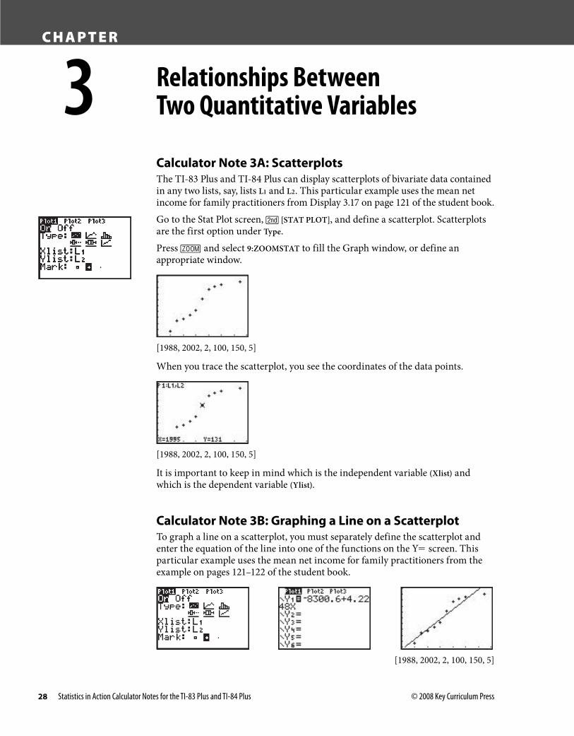
Calculator Note 3D: Finding ResidualsThe TI-83 Plus and TI-84 Plus will efficiently calculate residuals for any line of fit using the spreadsheet capabilities of the List Editor.a. First make sure that your data are entered into lists L1 and L2 and that the

equation of your fitted line is entered into the Y� screen.b. Define list L3 as the predicted y-coordinates, Y1(L1).

Calculator Note 3B (continued)


c. Then define list L4 as the residuals, L2–L3.

Alternatively, you could directly define list L3 as the residuals using the expression L2–Y1(L1).

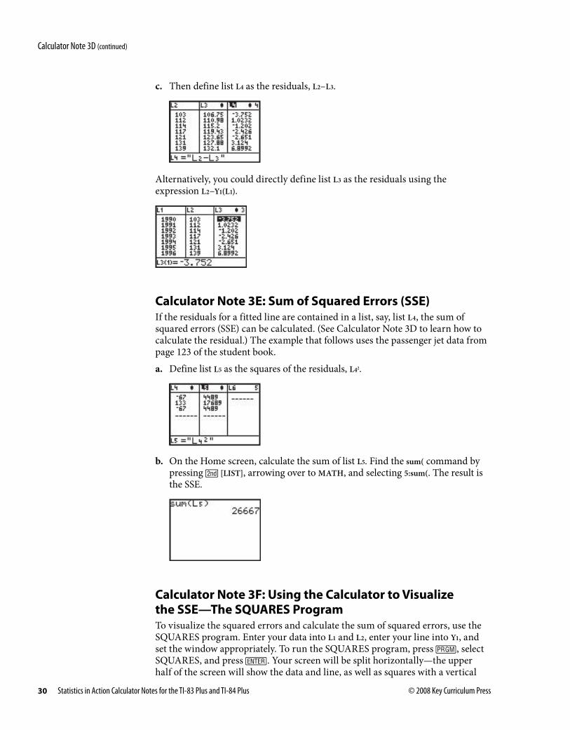
Calculator Note 3E: Sum of Squared Errors (SSE)If the residuals for a fitted line are contained in a list, say, list L4, the sum of squared errors (SSE) can be calculated. (See Calculator Note 3D to learn how to calculate the residual.) The example that follows uses the passenger jet data from page 123 of the student book.a. Define list L5 as the squares of the residuals, L 4 2 .

b. On the Home screen, calculate the sum of list L5. Find the sum( command by pressing y [LIST], arrowing over to MATH, and selecting 5:sum(. The result is the SSE.

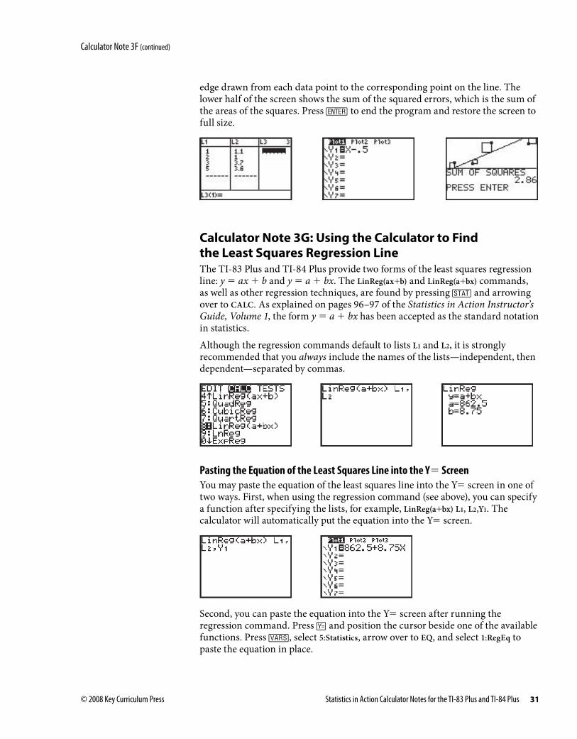
Calculator Note 3F: Using the Calculator to Visualize the SSE—The SQUARES ProgramTo visualize the squared errors and calculate the sum of squared errors, use the SQUARES program. Enter your data into L1 and L2, enter your line into Y1, and set the window appropriately. To run the SQUARES program, press è, select SQUARES, and press Õ. Your screen will be split horizontally—the upper half of the screen will show the data and line, as well as squares with a vertical

Calculator Note 3D (continued)


edge drawn from each data point to the corresponding point on the line. The lower half of the screen shows the sum of the squared errors, which is the sum of the areas of the squares. Press Õ to end the program and restore the screen to full size.

Calculator Note 3G: Using the Calculator to Find the Least Squares Regression LineThe TI-83 Plus and TI-84 Plus provide two forms of the least squares regression line: y � ax � b and y � a � bx. The LinReg(ax�b) and LinReg(a�bx) commands, as well as other regression techniques, are found by pressing Ö and arrowing over to CALC. As explained on pages 96–97 of the Statistics in Action Instructor’s Guide, Volume 1, the form y � a � bx has been accepted as the standard notation in statistics.Although the regression commands default to lists L1 and L2, it is strongly recommended that you always include the names of the lists—independent, then dependent—separated by commas.

Pasting the Equation of the Least Squares Line into the Y� ScreenYou may paste the equation of the least squares line into the Y� screen in one of two ways. First, when using the regression command (see above), you can specify a function after specifying the lists, for example, LinReg(a�bx) L1, L2,Y1. The calculator will automatically put the equation into the Y� screen.

Second, you can paste the equation into the Y� screen after running the regression command. Press o and position the cursor beside one of the available functions. Press ê, select 5:Statistics, arrow over to EQ, and select 1:RegEq to paste the equation in place.

Calculator Note 3F (continued)


Calculator Note 3H: Finding r and r 2 If you’d like the calculator to calculate and display the correlation, r, and coefficient of variation, r 2 , you must first turn Diagnostics on. Press yCATALOG, press É [D], arrow down to DiagnosticOn, and press Õ Õ. Now, when you perform a regression, the values of r 2 and r are shown.

A Formula for the Correlation, rIf desired, the spreadsheet capabilities of the List Editor can aid the calculation of the correlation. This process resembles Display 3.42 on page 142 of the student book.a. Enter the bivariate data into two lists, say, lists L1 and L2.b. Press Ö, arrow over to CALC, and select 2:2-VarStats and specify the lists.

Performing a 2-Var Stats calculates and stores the means, _ x and _ y , the standard deviations, Sx and Sy, and the number of data values, n. All of these variables can now be accessed by pressing ê, and selecting 5:Statistics.

c. Press Ö and select 1:Edit to return to the List Editor screen.d. Define list L3 with the expression L1 �

__ X /Sx.

e. Define list L4 with the expression L2 � __

Y /Sy.

f. Define list L5 with the expression L3*L4.g. On the Home screen, enter sum(L5)Y(n�1). The result is the correlation, r. Find

sum( by pressing y [LIST], arrowing over to MATH, and selecting 5:sum(.

Calculator Note 3G (continued)


Alternatively, after running the 2-Var Stats, you can calculate r directly on the Home screen by entering sum(((L1�

_ x )/Sx)((L2�

_ y )/Sy))/(n�1).

Calculator Note 3I: Residual PlotsEach time a TI-83 Plus or TI-84 Plus performs a regression, the calculator automatically computes the residuals and stores them in a list called RESID. Access this list by pressing y [LIST] and looking in the NAMES menu.Note that you can easily verify a necessary condition of residuals—that they sum to zero—by summing the values in RESID.You can easily make a residual plot by creating a scatterplot with RESID as the Ylist. Here are the original plot and the residual plot for the data on percentage of on-time arrivals versus mishandled baggage from Display 3.68 on page 169 of the student book.

[3.5, 8.5, 1, 65, 85, 5]

[3.5, 8.5, 1, –10, 10, 2]

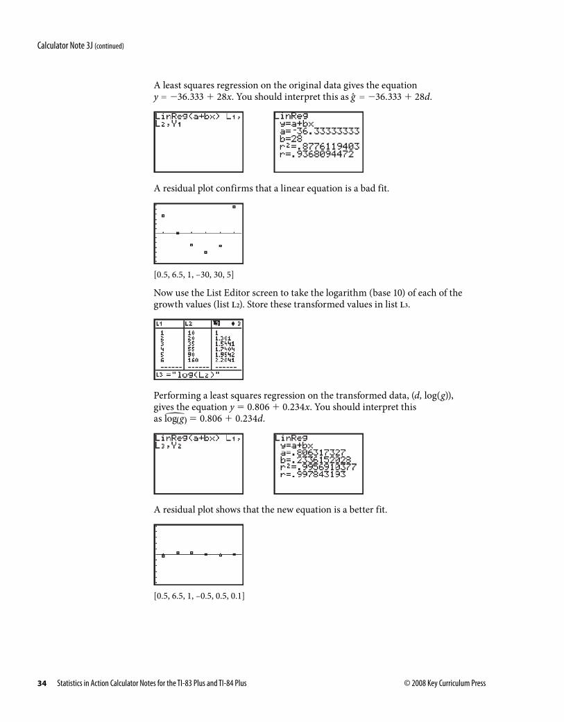
Calculator Note 3J: Shape-Changing TransformationsThe TI-83 Plus and TI-84 Plus can accomplish all of the transformations that are discussed in Section 3.5. However, the calculator always returns the coefficients of an equation in the form y � a � bx. It is up to you to note which transformations were used on which variables. For example, consider this small hypothetical data set that appears to exhibit an exponential relationship. Assume this data set relates days and growth, or data points in the form (d, g).

[0.5, 6.5, 1, �15.5, 185.5, 1]

Calculator Note 3H (continued)


A least squares regression on the original data gives the equation y � �36.333 � 28x. You should interpret this as g � �36.333 � 28d.

A residual plot confirms that a linear equation is a bad fit.

[0.5, 6.5, 1, –30, 30, 5]

Now use the List Editor screen to take the logarithm (base 10) of each of the growth values (list L2). Store these transformed values in list L3.

Performing a least squares regression on the transformed data, (d, log(g)), gives the equation y � 0.806 � 0.234x. You should interpret this as log � g � � 0.806 � 0.234d.

A residual plot shows that the new equation is a better fit.

[0.5, 6.5, 1, –0.5, 0.5, 0.1]

Calculator Note 3J (continued)

3 relationships between two quantitative variables€¦ · relationships between two quantitative...

Documents