Perceptron Learning; Maximum Margin Classifiers 13

3 Perceptron Learning; Maximum Margin Classifiers

Perceptron Algorithm (cont’d)

Recall:– linear decision fn f (x) = w · x (for simplicity, no ↵)– decision boundary {x : f (x) = 0} (a hyperplane through the origin)– sample points X1, X2, . . . , Xn 2 Rd; classifications y1, . . . , yn = ±1– goal: find weights w such that yiXi · w � 0– goal, rewritten: find w that minimizes R(w) =

Pi2V �yiXi · w [risk function]

where V is the set of indices i for which yiXi · w < 0.

[Our original problem was to find a separating hyperplane in one space, which I’ll call x-space. But we’vetransformed this into a problem of finding an optimal point in a di↵erent space, which I’ll call w-space. It’simportant to understand transformations like this, where a geometric structure in one space becomes a pointin another space.]

Objects in x-space transform to objects in w-space:

x-space w-spacehyperplane: {z : w · z = 0} point: wpoint: x hyperplane: {z : x · z = 0}

Point x lies on hyperplane {z : w · z = 0}, w · x = 0, point w lies on hyperplane {z : x · z = 0} in w-space.

[So a hyperplane transforms to its normal vector. And a sample point transforms to the hyperplane whosenormal vector is the sample point.]

[In this case, the transformations happen to be symmetric: a hyperplane in x-space transforms to a point inw-space the same way that a hyperplane in w-space transforms to a point in x-space. That won’t always betrue for the weight spaces we use this semester.]

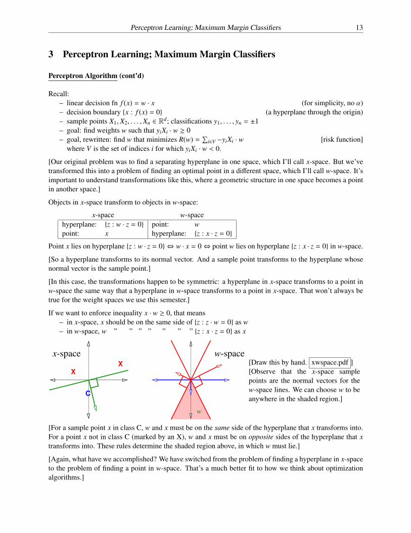
If we want to enforce inequality x · w � 0, that means– in x-space, x should be on the same side of {z : z · w = 0} as w– in w-space, w ” ” ” ” ” ” ” {z : x · z = 0} as x

C

X

X

w

x-space w-space[Draw this by hand. xwspace.pdf ][Observe that the x-space samplepoints are the normal vectors for thew-space lines. We can choose w to beanywhere in the shaded region.]

[For a sample point x in class C, w and x must be on the same side of the hyperplane that x transforms into.For a point x not in class C (marked by an X), w and x must be on opposite sides of the hyperplane that xtransforms into. These rules determine the shaded region above, in which w must lie.]

[Again, what have we accomplished? We have switched from the problem of finding a hyperplane in x-spaceto the problem of finding a point in w-space. That’s a much better fit to how we think about optimizationalgorithms.]

14 Jonathan Richard Shewchuk

[Let’s take a look at the risk function these three sample points create.]

-4 -2 0 2 4

-4

-2

0

2

4

riskplot.pdf, riskiso.pdf [Plot & isocontours of risk R(w). Note how R’s creases match thedual chart above.]

[In this plot, we can choose w to be any point in the bottom pizza slice; all those points minimize R.]

[We have an optimization problem; we need an optimization algorithm to solve it.]

An optimization algorithm: gradient descent on R.

Given a starting point w, find gradient of R with respect to w; this is the direction of steepest ascent.Take a step in the opposite direction. Recall [from your vector calculus class]

rR(w) =

2666666666666666664

@R@w1@R@w2...@R@wd

3777777777777777775

and r(z · w) =

26666666666666664

z1z2...

zd

37777777777777775= z

rR(w) =X

i2Vr � yiXi · w = �

X

i2VyiXi

At any point w, we walk downhill in direction of steepest descent, �rR(w).

w arbitrary nonzero starting point (good choice is any yiXi)while R(w) > 0

V set of indices i for which yiXi · w < 0w w + ✏

Pi2V yiXi

return w

✏ > 0 is the step size aka learning rate, chosen empirically. [Best choice depends on input problem!]

[Show plot of R again. Draw the typical steps of gradient descent.]

Problem: Slow! Each step takes O(nd) time. [Can we improve this?]

Perceptron Learning; Maximum Margin Classifiers 15

Optimization algorithm 2: stochastic gradient descent

Idea: each step, pick one misclassified Xi;do gradient descent on loss fn L(Xi · w, yi).

Called the perceptron algorithm. Each step takes O(d) time.[Not counting the time to search for a misclassified Xi.]

while some yiXi · w < 0w w + ✏ yiXi

return w

[Stochastic gradient descent is quite popular and we’ll see it several times more this semester, especiallyfor neural nets. However, stochastic gradient descent does not work for every problem that gradient descentworks for. The perceptron risk function happens to have special properties that guarantee that stochasticgradient descent will always succeed.]

What if separating hyperplane doesn’t pass through origin?Add a fictitious dimension.

Hyperplane: w · x + ↵ = 0

[w1 w2 ↵] ·

2666666664

x1x21

3777777775 = 0

Now we have sample points in Rd+1, all lying on plane xd+1 = 1.

Run perceptron algorithm in (d + 1)-dimensional space.

[The perceptron algorithm was invented in 1957 by Frank Rosenblatt at the Cornell Aeronautical Laboratory.It was originally designed not to be a program, but to be implemented in hardware for image recognition ona 20 ⇥ 20 pixel image. Rosenblatt built a Mark I Perceptron Machine that ran the algorithm, complete withelectric motors to do weight updates.]

Mark I perceptron.jpg (from Wikipedia, “Perceptron”) [The Mark I Perceptron Machine.This is what it took to process a 20 ⇥ 20 image in 1957.]

16 Jonathan Richard Shewchuk

[Then he held a press conference where he predicted that perceptrons would be “the embryo of an electroniccomputer that [the Navy] expects will be able to walk, talk, see, write, reproduce itself and be conscious ofits existence.” We’re still waiting on that.]

[One interesting aspect of the perceptron algorithm is that it’s an “online algorithm,” which means that ifnew data points come in while the algorithm is already running, you can just throw them into the mix andkeep looping.]

Perceptron Convergence Theorem: If data is linearly separable, perceptron algorithm will find a linearclassifier that classifies all data correctly in at most O(R2/�2) iterations, where R = max |Xi| is “radius ofdata” and � is the “maximum margin.”[I’ll define “maximum margin” shortly.]

[We’re not going to prove this, because perceptrons are obsolete.]

[Although the step size/learning rate doesn’t appear in that big-O expression, it does have an e↵ect on therunning time, but the e↵ect is hard to characterize. The algorithm gets slower if ✏ is too small because it hasto take lots of steps to get down the hill. But it also gets slower if ✏ is too big for a di↵erent reason: it jumpsright over the region with zero risk and oscillates back and forth for a long time.]

[Although stochastic gradient descent is faster for this problem than gradient descent, the perceptron algo-rithm is still slow. There’s no reliable way to choose a good step size ✏. Fortunately, optimization algorithmshave improved a lot since 1957. You can get rid of the step size by using any decent modern “line search” al-gorithm. Better yet, you can find a better decision boundary much more quickly by quadratic programming,which is what we’ll talk about next.]

MAXIMUM MARGIN CLASSIFIERS

The margin of a linear classifier is the distance from the decision boundary to the nearest sample point.What if we make the margin as wide as possible?

CX

X

X

X

X

X

C

C

CC

C

w · x + ↵ = 1w · x + ↵ = 0w · x + ↵ = �1 [Draw this by hand. maxmargin.pdf ]

We enforce the constraints

yi (w · Xi + ↵) � 1 for i 2 [1, n]

[Notice that the right-hand side is a 1, rather than a 0 as it was for the perceptron algorithm. It’s not obvious,but this a better way to formulate the problem, partly because it makes it impossible for the weight vector wto get set to zero.]

Perceptron Learning; Maximum Margin Classifiers 17

Recall: if |w| = 1, signed distance from hyperplane to Xi is w · Xi + ↵.Otherwise, it’s w

|w| · Xi +↵|w| . [We’ve normalized the expression to get a unit weight vector.]

Hence the margin is mini1|w| |w · Xi + ↵| � 1

|w| . [We get the inequality by substituting the constraints.]

There is a slab of width 2|w| containing no sample points [with the hyperplane running along its middle].

To maximize the margin, minimize |w|. Optimization problem:Find w and ↵ that minimize |w|2subject to yi(Xi · w + ↵) � 1 for all i 2 [1, n]

Called a quadratic program in d + 1 dimensions and n constraints.It has one unique solution! [If the points are linearly separable; otherwise, it has no solution.]

[A reason we use |w|2 as an objective function, instead of |w|, is that the length function |w| is not smooth atzero, whereas |w|2 is smooth everywhere. This makes optimization easier.]

The solution gives us a maximum margin classifier, aka a hard margin support vector machine (SVM).

[Technically, this isn’t really a support vector machine yet; it doesn’t fully deserve that name until we addfeatures and kernels, which we’ll do in later lectures.]

[Let’s see what these constraints look like in weight space.]

-1.0 -0.8 -0.6 -0.4 -0.2w2

-1.0

-0.5

0.5

1.0alpha

weight3d.pdf, weightcross.pdf [This is an example of what the linear constraints look likein the 3D weight space (w1,w2,↵) for an SVM with three training points. The SVM islooking for the point nearest the origin that lies above the blue plane (representing an in-class training point) but below the red and pink planes (representing out-of-class trainingpoints). In this example, that optimal point lies where the three planes intersect. At rightwe see a 2D cross-section w1 = 1/17 of the 3D space, because the optimal solution lies inthis cross-section. The constraints say that the solution must lie in the leftmost pizza slice,while being as close to the origin as possible, so the optimal solution is where the threelines meet.]