3 land allocation understanding land-use change (luc

2016 Billion-Ton Report | 37

3Land Allocation and Management: Understanding Land-Use Change (LUC) Implications under BT16 Scenarios

Keith L. Kline,1 Maggie R. Davis,1 Jennifer B. Dunn,2 Laurence Eaton,1 and Rebecca A. Efroymson.1

1 Oak Ridge National Laboratory2 Argonne National Laboratory

LAnd ALLoCAtIon And MAnAgeMent: UnderStAndIng LAnd-USe ChAnge (LUC) IMpLICAtIonS Under Bt16 SCenArIoS

38 | 2016 Billion-Ton Report

3.1 Introduction

3.1.1 Objectives The objective of this chapter is to help readers interpret results from the 2016 U.S. Billion-Ton Report (BT16) volume 1 related to the phenomena generally called “land-use change” (LUC) and “indirect land-use change” (ILUC). LUC can be described as a “change in the use or management of land by humans” (ISO 2015; IPCC 2000). However, definitions of LUC have varied widely in the literature (see appendix 3-A). In this chapter, unless specified otherwise, LUC refers to the effects on land that are caused or implied by the biomass production systems simulated in BT16. We describe where, how much, and what type of LUC is associated with the simulations.

The following questions and responses illustrate chapter goals and content:

• Why is analysis of LUC included in the BT16 volume 2? ▪ LUC is an important concern that can determine the acceptability of bioenergy, and current U.S. policies

call for monitoring and reporting on environmental effects of biofuel pathways inclusive of LUC. ▪ LUC effects are far-reaching and can be measured across all environmental indicators (see chapter 1).

• What are the LUC implications of BT16? ▪ LUC effects associated with any simulation are determined by model input parameters and assumptions,

and are distinctive for each scenario. ▪ BT16 scenarios apply constraints that prohibit net change in the total area of major land classes so that

the total area and extent of forestland and agricultural land are held constant throughout all simulations and time periods.

▪ Because total forest and agriculture land areas remain fixed, the most significant LUC effects relevant for environmental assessment under BT16 scenarios involve changes in land management practices.

▪ Building on continued trends of yield improvement and cropland area reduction, a principal manifes-tation of LUC is the net reduction in annual crops, which are replaced by idle land and perennial cover within the fixed agricultural area.

▪ Under BT16 scenarios at $60 per dry ton or less, by 2040, the area in perennial cover increases com-pared to the agricultural baseline in 2015 by ◦ 24 million acres under the base case (BC1) ◦ 45 million acres under the 3%-yield annual growth case (HH3).

▪ Under the same scenarios, the area in annual crops falls compared to the agricultural baseline in 2015 by ◦ 34 million acres under the base case (BC1) ◦ 55 million acres under the 3%-yield annual growth case (HH3).

▪ Approximately 10 million acres allocated to annual crops in the agricultural baseline in 2015, transitions to idle land under the BT16 scenarios.


• What other LUC issues are relevant to BT16? ▪ It is essential to understand the differences

between studies designed to estimate pol-icy-driven LUC and resource assessments such as BT16 that examine potential biomass supplies under specified conditions.

▪ The assumptions and constraints used in BT16 illustrate spatially explicit biomass supplies while excluding most potential LUC concerns by design.

▪ Estimates of change always depend on the reference case, and in this chapter we con-sider the BC1 simulation in 2017, and the agricultural baseline (described in volume 1) in 2015, 2017, and 2040, as references.

▪ BT16 does not simulate other references or define a “business as usual” case for 2040. However, other possible reference case con-siderations are discussed in appendix 3-A.

▪ Replicable methods to measure land-related effects are essential for science-based analy-sis of biomass production systems.

▪ Further research is required to clarify LUC effects of U.S. biomass production systems under different supply, demand, and policy scenarios.

3.1.2 The Importance of LUC and Related IndicatorsLUC is important because all other environmen-tal indicators, many of which are addressed in this report, as well as social and economic indicators, can be impacted by LUC (McBride et al. 2011; Dale et al. 2013). Under the Renewable Fuel Standard, LUC and indirect effects caused by U.S. biofuel policy must be considered. Since 2008, the effects of LUC have dominated discussion of environmental im-pacts of bioenergy because of their implications for greenhouse gas (GHG) emissions, biodiversity, food security, and other aspects of the environment.

The scientific literature identifies two LUC-related issues of high concern: (1) potential loss of areas of high conservation value, such as forests, peatland, wetlands, and native prairies; and (2) potential loss of agricultural output or displacement of cropland. The first type of potential LUC has implications for bio-diversity, GHG emissions, carbon stocks and seques-tration rates, and other environmental indicators, as discussed in this volume. The second type of poten-tial impact has implications for food security, as dis-cussed in the literature (e.g., GFMG 2010; Durham, Davies, and Bhattacharyya 2012; IFPRI 2015; Kline et al. 2016), as well as indirect effects. Chapter 2 discusses how BT16 applies modeling assumptions and constraints designed to estimate potential U.S. biomass supplies while controlling for and mitigat-ing these two specific concerns. In this chapter, we focus on LUC implications of the land management practices assumed in association with BT16 scenar-ios. As discussed in other chapters, changes in crop type and management are expected to affect most environmental indicators and especially those for soil carbon, GHG and air emissions, water quality, and biodiversity.

3.2 Research Goals Guide Choices for Model Parameters, Assumptions, and DefinitionsDifferent land input parameters and assumptions are applied to answer different questions about land and bioenergy (Dale and Kline 2013a). Many studies have aimed to address questions about the potential effects of a defined biofuel policy on land use (e.g., Fritsche and Wiegmann 2011; Fritsche, Sims, and Monti 2010; Oladosu et al. 2012; Oladosu and Kline 2013; Plevin et al. 2015; Valin et al. 2015; Taheripour and Tyner 2013; Tyner et al. 2010). LUC estimates



under specified scenarios require assumptions about relationships among productivity, prices, different commodity markets, and land (characterized by types, costs, locations, ownership, markets, etc.). LUC modeling studies are based on the assumption that biomass production will displace other produc-tion or other specific land uses.

3.2.1 The Differences between BT16 and Analyses that Focus on LUC BT16 is not an LUC study. Rather, BT16 describes domestic biomass resource potential with specific limitations on displacing other production (see de-tailed discussion in section 3.4 below). BT16 address-es questions about the locations and types of potential biomass within fixed agricultural and forestland areas and under scenarios that provide supplies not only for biomass, but for other projected agricultural and forestry market demands. BT16 scenarios are neutral about end use (i.e., the potential biomass supplies could be used for any purpose) and biofuel or other policies. While existing policies are implicitly reflect-ed in the USDA baseline projections (USDA 2015a), the U.S. Forest Products Module of the Global Forest Products Model (see chapter 2), and the BT16 agri-cultural baselines developed for BT16 scenarios (see chapter 2), BT16 supply simulations aim to illustrate prospective sources of biomass independent of any particular bioenergy policy.

BT16 aims to estimate how much biomass could be supplied from current agriculture and forestland in the conterminous United States under supply con-straints that limit typical LUC concerns, such as the loss of forests due to cropland expansion. U.S. for-estland area and U.S. cropland area are held constant in all scenarios. No land is allowed to transition from forestland to cropland under the simulations. Fur-thermore, all USDA Conservation Reserve Program (CRP) lands are excluded from biomass production (see BT16 volume 1, chapter 4). Assumptions and

constraints applied in BT16 scenarios mitigate po-tential market-mediated, global LUC effects, such as potential impacts on forests outside the United States (see chapter 2), and determine land allocation among crops and land cover. Understanding how these mod-el specifications influence land allocation is relevant for LUC estimates and for the interpretation of envi-ronmental effects. In summary, the BT16 scenarios il-lustrate future biomass potential from the agricultural and forestland bases as of 2015 and hold those areas constant for each simulation through 2040.

3.2.2 Concepts and Definitions Relevant to LUC The state of the art for LUC analysis reflects both operational and conceptual limitations associated with terms, definitions, and associated land classifi-cations used for analysis. Operationally, key terms used widely in the LUC and ILUC literature are often poorly defined, as many have acknowledged in the literature (e.g., Dale and Kline 2013a; ISO 2015; Kline, Oladosu, et al. 2011; Valin et al. 2015; Warner et al. 2014). Conceptually, LUC estimates from mod-els are limited by reliance on assumptions ranging from initial land classifications and attributes (includ-ing exclusivity of “use”) to the assumed causal driv-ers for transitions between classes (Efroymson et al. 2016). Large uncertainties in basic land cover classi-fications are well documented (e.g., Congalton et al. 2014; Kline, Parish, et al. 2011; Feddema et al. 2005; Emery et al. 2017). The classification uncertainties increase when land “use” is inferred from land cover classes (Lambin, Geist, and Lepers 2003), and uncer-tainties are inherently far greater still whenever an analysis attempts to quantify “change” (O’Hare et al. 2010; Dale and Kline 2013a; Dunn et al. 2017). Even more controversial are assumptions about causal drivers of LUC, such as the interaction of temporary price changes in commodity markets with many other known causal factors of deforestation (Efroymson et al. 2016; Aoun, Gabrielle, and Gagnepain 2013; Kline et al. 2016).


Every analysis that attempts to consider LUC is a product of underlying input data and assumptions, including how land classes and land use are defined (Dale and Kline 2013a; Woods et al. 2015). BT16 is no exception, although the goal of volume 1 was to estimate potential sustainable supplies rather than to perform an LUC analysis. BT16 focuses on biomass potential within the major land classes—agriculture and forestry—in the United States and builds on the best available USDA data sets for these two sectors. BT16 biomass potential is estimated under constraints that do not permit net changes in the land base over time for primary uses (e.g., forest to cropland) but rather involve changes in specified management over time on existing agriculture and forest domains. This makes BT16 distinct from other studies that attempt to define and parameterize land classes and to differentiate the services provided to society over space and time according to the classification system utilized. Models attempting to estimate LUC simplify data out of necessity, for example, by aggregating dynamic, heterogeneous uses into single classes for analysis (e.g., crop, pasture, forest, or urban). Relying on simplified land classes to assess LUC and gener-alizing characteristics of each class can be mislead-ing and detracts from science-based assessment and communication of verifiable impacts.

3.2.3 LUC and Biomass from ForestlandSee chapter 2 for a description of methods and assumptions applied to estimate potential biomass supplies from the forestry sector. The potential for the most significant LUC drivers associated with forest-ry biomass (e.g., loss of natural forest) is excluded from BT16 by design because the Forest Sustainable and Economic Analysis Model (1) aims to assure that demands for conventional wood products were met, in addition to those for biomass; (2) assumes no changes in areas for total timberland, plantations, and natural forest management lands; and (3) incor-

Text Box 3.1 | BT16 Land Terms and Major Crops Relevant to LUC

Key terms are defined in the glossary. The terms

“biomass” and “potential biomass supply” are

used without assumptions about end use. This is

in contrast to many biofuel LUC assessments that

estimate effects of a policy or production level

specified for bioenergy. In this chapter, the term

“bioenergy” is used in examples that aim to make

the discussion relevant to U.S. Department of

Energy Bioenergy Technologies Office stakeholders.

Moreover, scenarios in 2040 involve biomass “energy

crops,” so named because they are likely to be used

for energy purposes.

Agricultural land can be classified as annual crops

versus perennial cover, or as biomass (energy)

crops versus traditional (commodity) crops. For

our calculations of change in land cover and

management, idle land and Conservation Reserve

Program (see glossary) lands are excluded.

Traditional crops, such as corn and wheat, can supply

stover or straw (biomass); however, these are not

energy crops as defined by the U.S. Department of

Agriculture (USDA) because their primary end uses

are not for bioenergy. Agriculture simulations are

based on the Policy Analysis System model (see

chapter 2) using the following USDA major crops

(parenthetical values next to each crop indicate

millions of acres in 2015, the initial simulation year

of the agricultural baseline): corn (88), soybeans

(84), hay (58), wheat (all types, 56), cotton (10),

grain sorghum (7), barley (3), oats (3), and rice (3).

Forest-sector simulations are based on the Forest

Sustainable and Economic Analysis Model (see

chapter 2) to estimate potential supplies based on

timberlands in the United States.



porates supply constraints reflecting considerations, such as no new road building and limits or exclusions for biomass removals depending on terrain slope. As with agriculture lands, if less-restrictive assumptions are applied, larger potential biomass supplies could be simulated, but additional environmental issues would also be expected to arise.

Furthermore, BT16 does not consider the fact that some historic cropland is in transition to become for-est due to afforestation incentives provided under the CRP and similar programs. Because BT16 scenarios aim for supply potential that reflects some sustain-ability principles, all CRP lands were reserved and excluded from consideration in scenarios.

Thus, the estimates of biomass from the forestry sec-tor are meant to be conservative and avoid significant LUC concerns. Potential effects of alternative forest management approaches on the existing forestland, (e.g., water quality, habitat for selected species) are discussed in other chapters of BT16 volume 2. The remainder of this chapter focuses on the changes simulated on agriculture land.

One LUC effect relevant to forest cover is the in-creasing use of cropland for short-rotation woody crops (SRWCs). For the purposes of this analysis, these are treated as changes in management prac-tices on existing agricultural lands because, after a short rotation, the lands could rotate back into other agricultural uses. For example, as shown in table 3.1, by 2040 in HH3 case, 11 million acres of cropland are planted in SRWCs that can be coppiced (e.g., willow, eucalyptus), and an additional 13 million acres of cropland are planted in other SRWCs (e.g., poplar, pine). These changes in land management are discussed separately as one type of LUC within the agriculture sector.

3.3 Indicators to Capture LUC EffectsTo understand environmental effects of biomass pro-duction on land, clearly defined indicators and units are required to characterize and measure changes over space and time (McBride et al. 2011). The broad definition of LUC is nearly impossible to apply with consistency because any action or inaction of humans that potentially impacts land could be described as LUC. Furthermore, major changes in land qualities can occur within a forest or agriculture landscape without reaching a specified threshold for a defined change in cover class (a common proxy for LUC in modeling), such as forest/pasture or pasture/cropland. Therefore, specific indicators that permit consistent measurement of pertinent characteristics (i.e., of effects that stakeholders care about) are essential. Ex-amples of indicators relevant to LUC include carbon stocks and net primary productivity or biomass yield. While these are not measures of LUC per se, they are examples of indicators that capture the effects of different land management practices and production systems. Soil carbon is discussed in chapter 4. This chapter reviews how the amount of land managed for annual crops, pasture, and other perennial crops varies under different scenarios.

Two important conclusions about the use of LUC information to estimate environmental effects can be drawn from extensive literature and field work (e.g., Gasparatos et al. 2017): (1) what matters is what really changes rather than general land labels used for land classification, and (2) different manage-ment practices within a defined land class can lead to significant changes over time in measured values for environmental indicators (e.g., carbon stocks, biodiversity, water quality). For example, Fargione et


al. (2008) illustrate how the estimation of effects of bioenergy on carbon stocks depends on many factors independent of the basic land class used for LUC assessment. Forests range from degraded woodlands in dry environments to old-growth tropical forests. Carbon stocks and accumulation rates can vary by orders of magnitude while the land remains labeled as “forest.” The same holds true in agricultural sys-tems where, in addition to soils, weather, and prior use, the carbon stocks and sequestration rates depend on factors such as the type, timing and frequency of site preparation, fertilization, harvest, and soil tillage (e.g., specific equipment used, type and depth of tillage, area disturbed).

Biomass supplies in BT16 are sourced from the utili-zation of residues and coproducts from forestry and agriculture (e.g., timber thinning, corn stover), which are recognized in the literature to involve negligible potential for direct or indirect LUC (e.g., Fargione et al. 2008); biomass supplies in BT16 are also sourced through modifications of agricultural management practices, which influence environmental indicators over time. The incremental increases in biomass pro-duction under BT16 complement rather than displace current production. The assumptions and approach underlying BT16 reflect historical U.S. trends to im-prove land management efficiency in response to new and increasing biomass production. From 1984–2011,

for example, agricultural output increased by 1.5% per year while total area of land used for agriculture decreased by more than 0.5% per year, on average (Wang et al. 2015).

LUC-related effects that are estimated using indi-cators are a product of comparing BT16 scenarios (BC1 in 2017 and 2040 and HH3 in 2040) to each other and to the agricultural baseline in 2015, 2017, and 2040. Estimated effects always depend on the reference case, and many alternative future scenarios are possible (appendix 3-A). While BT16 scenarios exclude LUC between forestry and agriculture uses by design, and also exclude the use of CRP land for biomass crops, the scenarios involve changes in land management, crop type, and crop acreages within specific portions of the remaining agricultural landscape. The magnitude and implications of these changes are discussed below.

3.4 LUC and Agricultural Land: Cropland and PastureThe allocation of land among agricultural uses, including conventional crops, energy crops, and pe-rennial cover, is presented in table 3.1.



Table 3.1 | Crop Type, Cover Classification (Annual, Perennial, Idle), and Total Area in the Agricultural Baseline and in the BT16 Scenarios Considered in Volume 2

Agricultural Baseline

2015


2017

BC1 2017


2040

BC1 2040

HH3 2040

Crop Cover Class Millions of Acres

Barley Annual 3.5 3.2 3.2 2.9 2.8 2.7

Corn Annual 88 90 90 89 85 74

Cotton Annual 9.8 9.8 9.8 11 8.6 7.7

Oats Annual 3.0 2.5 2.5 2.4 2.1 1.9

Rice Annual 2.9 2.9 2.9 3.1 3.0 2.8

Sorghum Annual 7.5 7.4 7.4 7.0 6.2 5.8

Soybeans Annual 84 78 78 77 66 60

Wheat Annual 56 53 53 54 46 42

Total Major Crops 255 246 246 246 219 197

Hay Perennial 58 57 57 57 56 56

Idle Idle 13 22 22 23 23 23

Subtotal other cropland (idle, hay)

71 79 79 80 79 79

Total Cropland excl. energy crops

326 326 326 326 298 277

Total Pasture excl. energy crops

446 446 446 446 409 407

Bio-sorghum Annual 1.7 2.3

Coppice wood Perennial 5.0 11

Energy cane Perennial 0.0 0.3

Miscanthus Perennial 21 37

Non-coppice Perennial 9.3 13

Switchgrass Perennial 28 24

Total Energy Crops 0 0 0 0 64 88

Perennial 504 504 504 504 528 549

Annual 255 246 246 245 221 200

Idle 13 22 22 23 23 23

Total Agricultural Land Considered in BT16

772 772 772 772 772 772



2015


2017

BC1 2017


2040

BC1 2040

HH3 2040

Crop Cover Class Millions of Acres

Additional U.S. Agricultural Land:

Reserved CRP

Idle 27 27 27 27 27 27

Other farmland (woodlands, built up, roads, waste land, other)

110 110 110 110 110 110

Total farmland incl. CRP reserve

909 909 909 909 909 909

Table 3.1 summarizes total land allocation by class for the agricultural baseline in 2015, 2017, and 2040 to allow comparison with allocations under the BT16 scenarios analyzed in this volume. The land allocation data are consistent with U.S. farmland classifications as defined by the USDA National Agricultural Sta-tistics Service (NASS) (USDA NASS 2014) and as reported in the USDA baseline projections (USDA 2015a), with pasture categories combined in table 3.1. For comparison, note that the most recent Census of Agriculture (USDA NASS 2014) identified 914 million acres of total farmland, with 390 million in cropland (includes irrigated and cropland pasture); 415 million in other permanent pasture and range; 77 million in woodlands and grazed woodlands; and another 33 million acres in built-up areas, wasteland, or other non-productive uses of farmland. The smaller area considered in BT16 compared to the total USDA census (USDA NASS 2014) reflects reductions in cropland area based on the USDA baseline projections (USDA 2015a) and the exclusion of farmland outside the conterminous United States in BT16. The bottom rows of table 3.1 illustrate that 137 million acres were excluded from consideration in BT16 simulations be-fore the analysis began to apply constraints: 27 million acres of cropland in CRP were excluded, along with

110 million acres in built-up areas, wasteland, or other non-productive uses of farmland.

The differences in land allocation and management observed under different years and scenarios in table 3.1 include (1) increases in idle cropland area in all scenarios compared to the agricultural baseline in 2015; (2) decreases in conventional crop area in all scenarios compared to 2015; (3) decreases in pasture-land area in 2040 BT16 biomass scenarios compared to other scenarios; and (4) net increases in perennial land cover under BT16 biomass scenarios in 2040.

Idle cropland includes land allowed to go fallow for a period as part of normal rotations with other crops, as well as land available to support crops in response to market signals (see glossary). Because we do not assume idle cropland is managed exclusively as perennial or annual cover, idle remains a separate land class. For BT16 scenarios, 27 million acres of CRP are held constant and excluded from eligibility for any other use. By USDA’s definition, CRP falls into the “idle cropland” class. Thus, including the reserved CRP lands, there would be 50 million acres of idle cropland in the 2040 scenarios. LUC-related issues associated with different types of agricultural land management are discussed below.



3.4.1 Changes in Agricultural Land Management under BT16 ScenariosThe primary types of LUC associated with BT16 sup-ply scenarios involve changes in land management practices on land that has been in use for convention-al crops and pasture. The most significant net LUC from 2017 to 2040 is the transition from conventional annual crops to perennial land management systems, a transition that accelerates with increasing demand for biomass. The area estimated to be managed as perennial cover in 2040 is 45 million acres greater under the HH3 scenario than the area of perennial cover in the 2015 agricultural baseline or the 2040 agricultural baseline (see chapter 2) without new bio-mass demand. The geospatial distribution of the net change from annual to perennial cover is illustrated in figure 3.1 for BC1 2040 (reflecting a 24 million–acre expansion) and figure 3.2 for HH3 2040. The darker colors in figures 3.1 and 3.2 represent counties where perennial cover increased by 25%–40%. The light grey shading over most counties in the United States indicates that change was negligible or small (less than +/-5%). No counties have loss of perennial cover greater than 5% in 2040 under BT16 scenarios. Larger increases in percentage of perennial cover occur on agriculture land in areas where simulated returns from conventional crops are not as competi-tive with energy crops under the conditions defined in the base case scenario, BC1 2040.

The total land in perennial cover is about the same in the following scenarios: the agricultural baseline in 2015 and in 2017, the BC1 scenario in 2017, and the

agricultural baseline in 2040 (table 3.1). However, as with other land categories, while the total area in a class may appear to be constant across the nation over several years, this lack of net change can mask significant shifts in locations of perennial cover as well as net changes in any given county. In general, we observe that perennial cover increases incrementally in response to assumed biomass markets under BT16 scenarios.

The net expansion of perennial cover is significant in terms of land area (i.e., 24 to 45 million acres) but modest when considered relative to the overall agri-cultural landscape considered in the scenarios (772 million acres), as shown in figure 3.3. The expansion of idle cropland as a separate category in each sce-nario relative to the 2015 agricultural baseline is also illustrated in figure 3.3.

Figure 3.3 illustrates how total agricultural area managed as annual crops is estimated to decline and transition to perennial cover when the allocation of land in the agricultural baseline in 2015 is compared to land allocations in 2040 under (1) the agricultural baseline projection to 2040 without biomass demand; (2) BC1; and (3) HH3. Figure 3.3 illustrates the pro-gressively increasing amounts of land that transition on net from annual crops to perennial cover under these scenarios. The figure also illustrates that these shifts are small relative to the total agriculture land area considered in the analyses (772 million acres). Finally, note that in addition to the 27 million acres of CRP land reserved outside the analysis, the simu-lations include 23 million acres of idle land in each future scenario. The idle land provides a potential cushion, allowing response to unexpected increases in demand for crops or biomass in other sectors.


Figure 3.1 | Geospatial distribution of changes in perennial cover under the base case (BC1) scenario1

Figure 3.2 | Geospatial distribution of changes in perennial cover under the 3% annual yield increase (HH3) scenario1

Change in Perennial Cover as a Percent of Ag Acres (2040 vs. 2015)1% yield increase (BC1), $60/dry ton o�ered

> 35% change> 25% change> 15% change> 5% changeLess than 5% change or less than 1000 acres perennial


1 Change in perennial cover by county is the difference between the percentage of total agricultural acres (cropland + pasture) managed as perennial cover in BT16 2040 scenarios (BC1 or HH3) and the percentage managed as perennial cover in the 2040 agricultural baseline without new biomass production. In each scenario, the gray includes a few counties that transitioned to less than 1,000 acres of perennials in 2040. These are mostly urban areas and average less than 265 acres of planted perennials per county. For instance, this filter avoids showing Clayton County, Georgia, in the >35% change category, even though it went from 0 to 44 perennial acres out of a total of 106 planted acres.




Figure 3.3 | Agricultural land (millions of acres) managed as annual crops, perennial cover, or idle cropland in 2015 and 2040 as estimated under (a) the agricultural baseline; (b) base case scenario (BC1); and (c) high-yield scenario (HH3)

255 245 255 221 255 200

504

1323

204020152040201520402015

a. Agricultural Baseline b. Base-case (BC1) c. High-yield (HH3)

504 504 528 504 549

Annual Cover Idle (13 million rising to 23 million acres in each case) Perennial Cover

In addition to the gradual transition from row crops to perennial biomass crops illustrated in figure 3.1, changes in management occur on pasture. By 2040, 37–39 million acres, or about 8% of total pasture area in the 2015 extended agricultural baseline, would undergo changes in management to produce energy crops. This area is not segregated in figures 3.1–3.3, which compare annual crops to perennial cover, be-cause both pastureland and the energy crops illustrat-ed are classified as perennial cover.

The changes from annual to perennial land man-agement affect 3% of total agricultural land under BC1 and about 6% under HH3, and the transitions occur gradually between 2015 and 2040. There are also gradual changes in the management of pastures, with about 8% of total pastureland area in the 2015 agricultural baseline shifting to management for en-ergy crops by 2040. Fencing and pasture rotation are management practices that are assumed to intensify production on another 56–58 million acres of pasture (13% of total pastureland) to maintain forage output

in tandem with increasing energy crop production. Percentages here are expressed relative to the to-tal areas of cropland and pastureland in the 2015 agricultural baseline and the projected agricultural baseline in 2040 (table 3.1). As with any model, input parameters and assumptions regarding land classes, land area available for different uses, and productiv-ity influence how land is allocated among traditional and energy crops over time. Assumed increases over time in the productivity of pasture (see BT16 volume 1, section 4.8.5), yields for conventional and energy crops, and simulated prices of biomass are the drivers for the modeling results allowing for increased bio-mass feedstock production within the current (2015) agricultural landscape.

3.4.2 Land Input Assumptions Drive LUC Estimates The input values for land parameters and constraints relevant to LUC are described in chapter 2. Key pa-rameters impacting LUC include the initial land base


in POLYSYS, independent of assumed new biomass demand. For example, in the agricultural baseline scenario, the area planted in major crops is estimated to decrease by about 10 million acres while overall outputs increase through improved productivity.

In BT16 biomass scenarios, the area of agricultural land managed for annual crops in BC1 2040 is 25 million acres less that the quantity simulated in BC1 2017; and from BC1 2017 to HH3 2040, the decline is 46 million acres. Similar differences are observed if BC1 2040 and HH3 2040 are compared to the agricultural baseline in 2040 (table 3.1). However, the reduction in land area managed for annual crops is different if these scenarios are compared to the 2015 agricultural baseline (table 3.2), due primarily to decreased demand for commodity crops between 2015 and 2017. Most reductions in annual crop acreage over time can be accounted for by increased yields and decreased area planted in conventional crops (primarily soy beans, corn, and wheat; see table 3.1). As the area managed for conventional annual crops declines, the area managed as perennial cover increases along with increasing energy crop produc-tion.

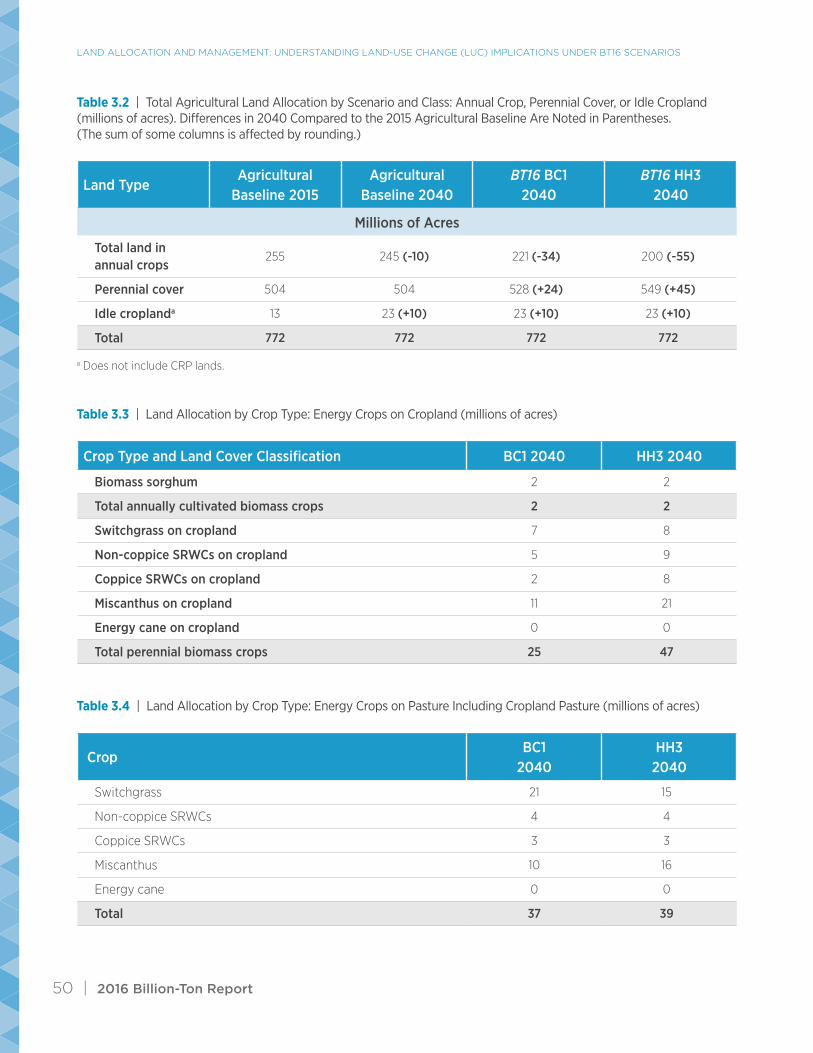
Table 3.2 highlights the net changes in land managed as annual crops, idle, and perennial cover when the 2015 agricultural baseline is compared to scenarios for 2040. Table 3.3 shows the allocation of 2015 cropland acres to specific biomass crops in 2040 under the two scenarios (BC1 and HH3). Table 3.4 illustrates the allocation of 2015 pastureland to bio-mass crops under the two scenarios.

and land classes considered, and the annual rates of expansion allowed. For example, energy crop acreage in a county is limited to 5% of permanent pasture, 20% of cropland pasture, and 10% of cropland. These percentages reflect an estimate of barriers and oppor-tunities associated with the adoption of new crops.

Before applying any constraints, an initial agricul-tural land base of 772 million acres was considered for BT16 biomass supply scenarios modeled in the Policy Analysis System (POLYSYS) (table 3.1). This acreage includes eight major row crops plus cultivat-ed hay on cropland, for a total of 313 million acres of cropland, plus 446 million acres of pasture. For BT16, pastureland includes 11 million acres classified as cropland pasture, plus other pasture and rangeland (figure 3.4). The definition of each class is based on the USDA 2012 Census of Agriculture (USDA NASS 2014; see glossary for full definitions), and the acre-ages in table 3.1 for cropland classes were based on average values reported over 4 years in recent NASS statistics (see appendix C of BT16 volume 1).

When interpreting any description of LUC, it is essential to understand that “change” is always ex-pressed with respect to the comparison of two select-ed values. Thus, LUC associated with BT16 varies depending on whether it is a product of comparing a given simulation (1) to another simulation (e.g., BC1 2040 versus HH3 2040), (2) to the agricultural base-line in 2015 or 2040 (table 3.2), (3) to different years within a given scenario (e.g., BC1 2017 versus BC1 2040), or (4) to some other reference case. Changes occur in the USDA baseline projections (USDA 2015a) and in the projected agricultural baseline simulated



Table 3.2 | Total Agricultural Land Allocation by Scenario and Class: Annual Crop, Perennial Cover, or Idle Cropland (millions of acres). Differences in 2040 Compared to the 2015 Agricultural Baseline Are Noted in Parentheses. (The sum of some columns is affected by rounding.)

Table 3.3 | Land Allocation by Crop Type: Energy Crops on Cropland (millions of acres)

Table 3.4 | Land Allocation by Crop Type: Energy Crops on Pasture Including Cropland Pasture (millions of acres)

Land Type Agricultural

Baseline 2015Agricultural

Baseline 2040BT16 BC1

2040BT16 HH3

2040

Millions of Acres

Total land in annual crops

255 245 (-10) 221 (-34) 200 (-55)

Perennial cover 504 504 528 (+24) 549 (+45)

Idle croplanda 13 23 (+10) 23 (+10) 23 (+10)

Total 772 772 772 772

Crop Type and Land Cover Classification BC1 2040 HH3 2040

Biomass sorghum 2 2

Total annually cultivated biomass crops 2 2

Switchgrass on cropland 7 8

Non-coppice SRWCs on cropland 5 9

Coppice SRWCs on cropland 2 8

Miscanthus on cropland 11 21

Energy cane on cropland 0 0

Total perennial biomass crops 25 47

CropBC1

2040HH3

2040

Switchgrass 21 15

Non-coppice SRWCs 4 4

Coppice SRWCs 3 3

Miscanthus 10 16

Energy cane 0 0

Total 37 39

a Does not include CRP lands.


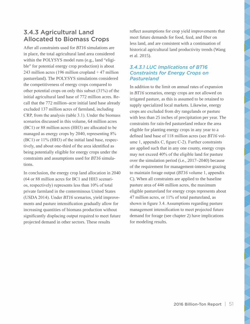
3.4.3 Agricultural Land Allocated to Biomass CropsAfter all constraints used for BT16 simulations are in place, the total agricultural land area considered within the POLYSYS model runs (e.g., land “eligi-ble” for potential energy crop production) is about 243 million acres (196 million cropland + 47 million pastureland). The POLYSYS simulations considered the competitiveness of energy crops compared to other potential crops on only this subset (31%) of the initial agricultural land base of 772 million acres. Re-call that the 772 million–acre initial land base already excluded 137 million acres of farmland, including CRP, from the analysis (table 3.1). Under the biomass scenarios discussed in this volume, 64 million acres (BC1) or 88 million acres (HH3) are allocated to be managed as energy crops by 2040, representing 8% (BC1) or 11% (HH3) of the initial land base, respec-tively, and about one-third of the area identified as being potentially eligible for energy crops under the constraints and assumptions used for BT16 simula-tions.

In conclusion, the energy crop land allocation in 2040 (64 or 88 million acres for BC1 and HH3 scenari-os, respectively) represents less than 10% of total private farmland in the conterminous United States (USDA 2014). Under BT16 scenarios, yield improve-ments and pasture intensification gradually allow for increasing quantities of biomass production without significantly displacing output required to meet future projected demand in other sectors. These results

reflect assumptions for crop yield improvements that meet future demands for food, feed, and fiber on less land, and are consistent with a continuation of historical agricultural land productivity trends (Wang et al. 2015).

3.4.3.1 LUC Implications of BT16 Constraints for Energy Crops on Pastureland

In addition to the limit on annual rates of expansion in BT16 scenarios, energy crops are not allowed on irrigated pasture, as this is assumed to be retained to supply specialized local markets. Likewise, energy crops are excluded from dry rangelands or pasture with less than 25 inches of precipitation per year. The constraints for rain-fed pastureland reduce the area eligible for planting energy crops in any year to a defined land base of 118 million acres (see BT16 vol-ume 1, appendix C, figure C-2). Further constraints are applied such that in any one county, energy crops may not exceed 40% of the eligible land for pasture over the simulation period (i.e., 2017–2040) because of the requirement for management-intensive grazing to maintain forage output (BT16 volume 1, appendix C). When all constraints are applied to the baseline pasture area of 446 million acres, the maximum eligible pastureland for energy crops represents about 47 million acres, or 11% of total pastureland, as shown in figure 3.4. Assumptions regarding pasture management intensification to meet projected future demand for forage (see chapter 2) have implications for modeling results.



Figure 3.4 | Total U.S. pastureland area and subset eligible for biomass crops (millions of acres). The constraints applied in BT16 reduce the area of pasture eligible for energy crops from a total of 446 million acres to 47 million acres (applica-ble to all scenarios, in all years).

Total Potential Pasture Unavailable: 399.3

Permanent Pasture(dry+irrigated): 291.1

Permanent Pasture(rainfed+non-irrigated): 291.1

Permanent Pasture: 402.1Total Pasture: 446.3

Cropland Pasture: 11.2

Other Pasture: 33.1Cropland Pasture (dry+irrigated): 4.4

Cropland Pasture (rainfed+non-irrigated): 6.8Total Potential Pasture Available: 47.1

3.4.3.2 Energy Crops on Cropland

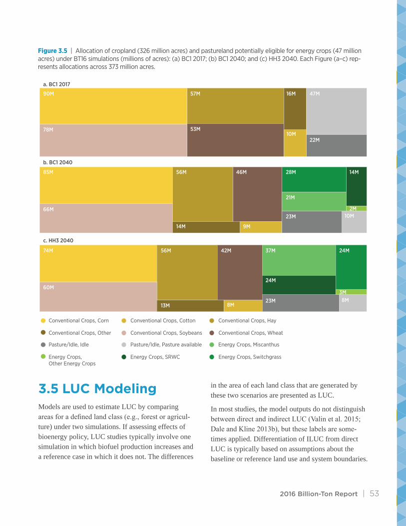
The cumulative effect of the BT16 constraints for ex-pansion of energy crops is that the maximum amount of cropland potentially eligible for energy crops by 2040 represents about half of the cropland area considered in the 2015 agricultural baseline and in BC1 2017. The cumulative expansion in 2040 of 27 million acres of energy crops in BC1 represents only about 8% of total 2015 cropland area (326 million acres) and 15% of the eligible cropland area under the constraints used in BT16 (27 million acres out of 181 million eligible). The high-yield scenario (HH3) results in a cumulative planting of energy crops by

2040 on 49 million acres of cropland, or about 15% of the 2015 agricultural baseline cropland area. As illustrated in figure 3.5, the allocation of cropland to row crops declines over time in BT16 scenarios in association with increasing biomass production. A gradual reduction in U.S. cropland area is consistent with historic trends and with the agricultural baseline projection that simulated a 10 million–acre reduction in cropland area from 2015 to 2017 (table 3.2). In part, the reduced area of cropland reflects the fact that total factor productivity of U.S. agriculture has been increasing while land as an input has been declining (Wang et al. 2015).


Figure 3.5 | Allocation of cropland (326 million acres) and pastureland potentially eligible for energy crops (47 million acres) under BT16 simulations (millions of acres): (a) BC1 2017; (b) BC1 2040; and (c) HH3 2040. Each Figure (a–c) rep-resents allocations across 373 million acres.

90M

a. BC1 2017

b. BC1 2040

c. HH3 2040

Conventional Crops, Corn Conventional Crops, Cotton Conventional Crops, Hay

Conventional Crops, Other Conventional Crops, Soybeans Conventional Crops, Wheat

78M 53M10M

57M 16M 47M

22M

85M 56M

14M

46M

9M

28M

21M

23M

14M

2M10M

66M

74M 56M

13M 8M

42M 37M

24M

23M

24M

3M8M

60M

Pasture/Idle, Idle Pasture/Idle, Pasture available Energy Crops, Miscanthus

Energy Crops, Other Energy Crops

Energy Crops, SRWC Energy Crops, Switchgrass

3.5 LUC ModelingModels are used to estimate LUC by comparing areas for a defined land class (e.g., forest or agricul-ture) under two simulations. If assessing effects of bioenergy policy, LUC studies typically involve one simulation in which biofuel production increases and a reference case in which it does not. The differences

in the area of each land class that are generated by these two scenarios are presented as LUC.

In most studies, the model outputs do not distinguish between direct and indirect LUC (Valin et al. 2015; Dale and Kline 2013b), but these labels are some-times applied. Differentiation of ILUC from direct LUC is typically based on assumptions about the baseline or reference land use and system boundaries.



For example, in the case of economic models exam-ining U.S. biofuel policies, LUC that occurs outside the United States is commonly labeled “indirect.” However, a study focusing on biomass production in a single U.S. state may consider LUC projected outside of that particular state to be indirect. Other studies attempt to allocate land areas based on an assumed initial land cover compared with a simulated land cover, wherein any land used for biomass pro-duction that is modeled to occur on non-agricultural land is considered a “direct LUC,” and the sum of all other changes in land use is assumed to be indirect.

The potential global impacts of an expansion of biomass production in the United States depend on many factors not analyzed under BT16 scenarios. Reasonable assumptions about increasing biomass production could generate estimates that vary wide-ly not only in terms of magnitude, but also in terms of direction of the effects—particularly in terms of whether forestland is expected to expand or contract in response to policies associated with biomass pro-duction (see appendix 3-A; Kline et al. 2009).

3.5.1 How BT16 Relates to Concerns about ILUCBT16 is not designed to address questions about LUC, but understanding how bioenergy policies actually interact with other policies, markets, and dis-turbances (such as fire) is critical for more accurate LUC assessment (Kline and Dale 2008). A review of the conceptual basis for LUC modeling can illustrate how common concerns about indirect effects are managed in BT16 with a focus on ILUC modeling. The two main forces assumed to drive ILUC are (1) price mechanisms and (2) crop displacement:

• Under the price mechanism, ILUC can occur if (1) biomass production causes higher prices for other commodities; (2) these higher prices are transmitted to markets in other countries; and

(3) the response in those countries to the higher prices is to clear more land for growing those crops than would have been cleared otherwise.

• Under the displacement mechanism, ILUC can occur if (1) biomass production displaces local output of a crop; (2) the reduced output of the crop is replaced by growing more of the crop elsewhere; and (3) growing more of the crop elsewhere requires the clearing of new agricul-tural land.

Both of these mechanisms require causal pathways (a b c…) in which the absence of any one step would block the effect (Efroymson et al. 2016). For example, under the first mechanism, if higher prices are not transmitted to other nations, or if higher pric-es cause intensification rather than new land clearing, then the pathway is interrupted and the assumed effect would be blocked. Empirical evidence suggests that such conditions may create breaks in the causal chain assumed for the price mechanism. Rather than testing for the existence of these mechanisms, eco-nomic models for ILUC typically begin by assuming the mechanisms are in place and then seek to assess effects of a “shock” in biofuel demand to generate ILUC estimates.

Regarding the two basic mechanisms above, BT16 constraints were applied to minimize these “mar-ket-mediated” effects. For the price mechanism, it is estimated under the BT16 supply scenarios that com-modity prices could be higher or lower depending on the rate of yield growth assumed (see BT16 volume 1, appendix C). Regardless of whether prices are pro-jected to decline or rise, the price changes associated with biomass production are small relative to other drivers of change in food commodity prices (Kline et al. 2016). More detailed analysis of the impacts of potentially higher or lower prices (depending on the BT16 scenario) on global markets and land use is beyond the scope of the analysis for this study.


Regarding potential crop displacement mechanisms, BT16 simulations were based on scenarios that allowed conventional commodity outputs to increase over time and fulfill increasing demand. The assumed incremental expansion of energy crops in tandem with increasing productivity reduces potential mech-anisms theorized to cause ILUC. Under the HH3 scenario, in which energy crops occupy the greatest area (88 million acres) by 2040, the land in row crops is simulated to decline by 56 million acres while total output continues to grow each year to meet or exceed demands projected under the 2040 agricultural base-line (see BT16 volume 1, appendix C). While corn stover is an important source of biomass in BC1 and HH3 simulations, acreage in corn and conventional crops overall decline in biomass production scenar-ios. These BT16 results are consistent with decadal trends, which show a small but steady reduction in conventional crop acreage over time. This study focuses on potential new cellulosic biomass supplies building from a 2015 agricultural baseline; it does not consider changes to current conventional biofuel programs (e.g., corn starch ethanol and soy-based biodiesel production).

The BT16 constraints aim to avoid biomass produc-tion locations, management practices, and economic competitions that would represent likely environmen-tal concerns (see chapters 1 and 2). This approach is consistent with other studies that investigate options to produce biomass while preventing or mitigating LUC and other environmental impacts (e.g., Brink-man et al. 2015; RSB 2015; Gerssen-Gondelach et al. 2016; Gerssen-Gondelach, Wicke, and Faaij 2015; Beringer, Lucht, and Schaphoff 2011; Schubert et al. 2009; Wicke et al. 2015). The assumptions applied to estimate potential biomass supplies that could be produced from current agricultural and forestlands without changing the areas now used for those broad categories are likely to be as accurate as (if not better than) alternative assumptions that attempt to predict how these land areas will change in the future (e.g., see Buchholz et al. 2014). Even though no one ex-

pects all current forestland acres to remain the same over the next 25 years, the BT16 assumption that net area does not change is defensible given the purpose of the assessment and historical trends (discussed below). No net change in area is a common ceteris paribus (all else held constant) modeling assumption that facilitates simulations by avoiding additional complications. Furthermore, the U.S. Renewable Fuel Standard (H.R. 6 2007) only considers biomass used for fuels to be renewable if it is derived from land cleared or cultivated for agriculture or managed forests prior to 2007. For more discussion of the assumptions underlying the agricultural baseline and how BT16 scenarios address projected future de-mand, see chapter 2 of BT16 volume 2 and appendix C of BT16 volume 1.

3.5.2 BT16 Results in Context of Other LUC StudiesIt is difficult to compare the BT16 resource assess-ment to other studies designed to estimate LUC, as the questions asked and approaches applied are distinct. However, it can be enlightening to carefully review the input parameters and assumptions un-derlying each approach to determine what is driving the results of a given simulation of future biomass production. Assumptions and details behind BT16 are carefully documented to support transparent analysis (see chapter 2).

Input data sets and assumptions are critical factors that determine LUC assessment results. The land class ontology, land areas and uses considered, and land rents assumed in a baseline are key factors, along with how spatially explicit land units are defined and how they are segregated or aggregated for analysis. These input specifications vary widely from study to study and are one of many sources of divergent LUC estimates. Further, the criteria and data used to differentiate land cover from land use, and to specify past productivity and potential future productivities at high resolution (not to mention



current carbon stocks and rates of net sequestration or emissions), are rarely documented but are also critical to many LUC effects assessments.

Modelers acknowledge that ILUC estimates cannot be validated (NRC 2011; Valin et al. 2015; Babcock 2009). Calibrating estimates of ILUC attributed to biomass production is challenging because (1) the LUC is not defined in practical, consistent, and verifi-able terms; (2) other confounding factors determine if and when observable changes, such as deforestation, occur around the world; (3) the processes involved are not singular events but rather reflect constant and ongoing incremental changes and dynamic cycles; and (4) to calibrate and validate models would require extensive and costly field analysis to support statistical analyses of all potential factors and support a defensible allocation of observed changes among countless causal agents (Efroymson et al. 2016; Valin et al. 2015; Kline et al. 2009). Even if all the data and statistical analyses could be completed, a reference case must be simulated in order to estimate “change,” and therefore, modeling assumptions are a necessity (NRC 2011).

Given high uncertainty and limitations of LUC models (Plevin et al. 2015; Verburg, Neumann, and Nol 2011; Aoun, Gabrielle, and Gagnepain 2013; Souza et al. 2015; Hertel et al. 2010; NRC 2014), it is important to examine underlying assumptions and input variables that drive LUC results for any study in order to understand and interpret results. Indeed, many assumptions used in past LUC model-ing for bioenergy have been found to be invalid (e.g., Babcock 2009; Kim and Dale 2011; Kline, Oladosu, et al. 2011; Dale and Kline 2013a), and there is little empirical evidence to support the types and magni-tudes of LUC that have been projected (Langeveld et al. 2014; Babcock and Iqbal 2014; Oladosu et al. 2011). Recent research suggests that the state of sci-ence is inadequate to include ILUC in international standards (Zilberman et. al., 2010; ISO 2015; ASTM 2016). As stated in a policy analysis report by the

National Research Council, the “range of estimates for GHG emissions from indirect land-use changes is wide…,” but “GHG emissions from land-use changes cannot be ignored…results by definition carry the assumptions and inherent uncertainties in these mod-els”; the report concludes that “[a]dditional research is needed to better understand the socioeconomic processes of land-use change and to integrate that process understanding into models” (NRC 2011). The caveat to carefully examine input specifications and assumptions is applicable to any analysis attempting to estimate impacts of future or alternative land man-agement, including BT16. Comparing input data and assumptions helps put land allocations from BT16 scenarios into a broader context of LUC analysis. See appendix 3-A for further discussion.

Estimating future LUC is difficult in part because of the controversies that surround analysis of past LUC. For example, some analyses begin by assuming that land in cropland subcategories—such as idle, hay, and cropland-pasture—are “non-agricultural” grassland in the baseline. It is then not surprising that these analyses identify large amounts of “grassland conversion” (e.g., Mladenoff et al. 2016; Wright and Wimberly 2013). However, based on USDA defini-tions, acres that such studies flag as “converted” are more accurately described as forming part of ongoing management and rotations on cropland because these lands were previously used and classified as culti-vated cropland (USDA NASS 2014; Kline, Singh, and Dale 2013; Qin et al. 2016; Johnston 2014). Further, managing idle, hay, and cropland-pasture land subcategories in rotation with row crops may be a preferable strategy to achieve ecosystem benefits (such as soil conservation, reductions in pests and the need for herbicides and pesticides, and soil moisture conservation) and to efficiently achieve other goals within constraints dictated by local circumstances. Regardless, under BT16, idle and hay are considered part of the cropland class, which is consistent with USDA definitions.


There is often not a clear line to separate grassland from pasture, or pasture from other cropland (see appendix 3-A). Alternating or coproducing row crops with perennial crops over long rotations is one of the many management complexities that makes anal-ysis of LUC difficult or misleading. Therefore, we recommend focusing on actual management practices and the specific effects of those practices on environ-mental indicators, rather than vague LUC labels for temporary changes in land management.

3.6 DiscussionIn this section, we review how BT16 simulations compare to historic LUC trends, discuss limitations and uncertainties inherent in LUC analysis, and propose some directions for future research. Because some type of LUC is constantly occurring practical-ly everywhere that humans are present and because LUC involves multiple ongoing interactions rather than a singular event, modeling LUC is a challenge. Therefore, LUC assessments must begin by clearly defining the question to be addressed, the type of LUC of concern, and the data to be used, and then applying an approach appropriate for the situation.

In the case of BT16, given the constraints that prohib-it net changes in total areas for forest and agriculture (and the reservation of 27 million acres for CRP within the agriculture land base), the LUC issues re-late to estimated land management changes and how the management practices and locations associated with biomass production compare to historic land management and alternative future scenarios. Above, we reviewed the BT16 scenarios compared to pro-jected future baseline scenarios. Below, we consider historical data and trends.

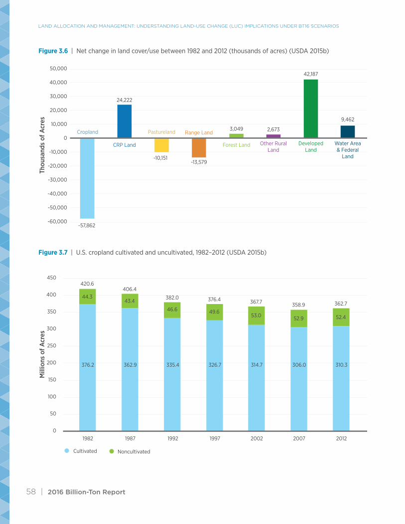
3.6.1 Land for Biomass Crops in Context of Historical Trends To place the BT16 land allocations in 2040 scenarios into perspective, consider that over the 30-year peri-od of 1982‒2012, U.S. agricultural output increased

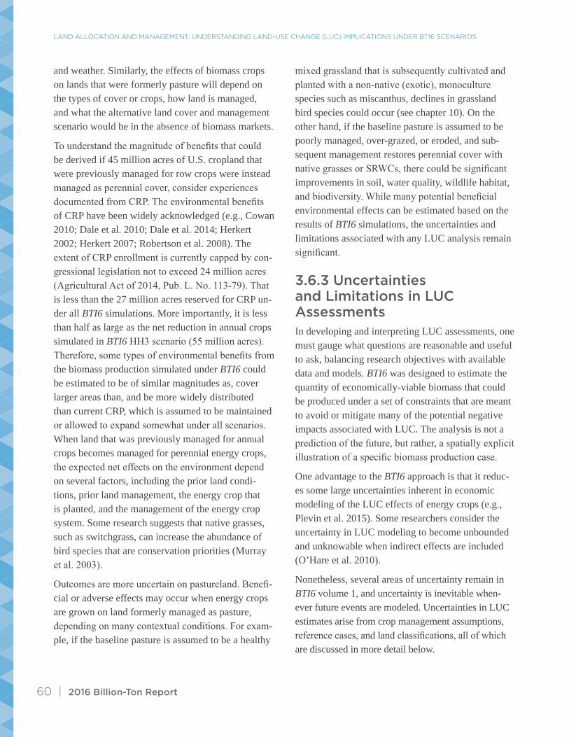
persistently at an average rate of 1.5% growth per year, while over the same time period, the land used as an input for agricultural production fell at an av-erage rate of 2.7 million acres per year—resulting in an 82 million–acre net reduction (summing cropland, pasture, and range), as shown in figure 3.6 (USDA 2015b). Focusing on the area of cultivated cropland, USDA analysis found that this input to production fell by 66 million acres, from 376.2 million in 1982 to 310.3 million in 2012, as illustrated in figure 3.7.

The ability to increase agricultural output while using less land over the past two decades is largely attribut-ed to “total factor productivity” improvements (figure 3.8; USDA ERS 2016a; Wang et al. 2015). System efficiency can improve by increasing coproducts and reducing wastes. Risks and costs are reduced by diversifying market options and increasing flexibility for substitution.

Future agricultural land-use trends will be influenced by many factors, including the impact of climate change on crop yields (chapter 13), commodity prices, and agricultural policies. Under the BT16 BC1 scenario, 64 million acres could be dedicated to biomass by 2040. This is similar to the acreage that could shift to non-agricultural uses if historical trends were to continue throughout the simulation period. However, future land-use trends may not follow past trends and are always uncertain. If new technologies and markets create incentives for cover crops, double crops, or higher yields, or if other mechanisms in-crease land-factor productivity, then less land will be required to meet future demand projections and more land would be available for other uses, including biomass. However, if yields do not grow as assumed in the BT16 scenarios, or if weather or markets disrupt production, or demands for commodity crops are higher than anticipated, then less land would be available. Thus, while BT16 simulations appear rea-sonable and are consistent with long-term historical trends for agricultural land management, actual future land use will be dependent on many factors.



Figure 3.6 | Net change in land cover/use between 1982 and 2012 (thousands of acres) (USDA 2015b)

Figure 3.7 | U.S. cropland cultivated and uncultivated, 1982–2012 (USDA 2015b)

Thou

sand

s of

Acr

es

-60,000

30,000

20,000

40,000

50,000

-40,000

-50,000

-10,000

-20,000

-30,000

10,000

0

-57,862

Cropland

24,222

CRP Land

3,049

Forest Land

2,673

Other RuralLand

42,187

DevelopedLand

9,462

Water Area& Federal

Land-10,151

Pastureland

-13,579

Range Land

Mill

ions

of A

cres

0

350

300

400

450

100

50

250

200

150

376.2

44.3

420.6

362.9

43.4

406.4

335.4

46.6

382.0

326.7

49.6

376.4

314.7

53.0

367.7

306.0

52.9

358.9

310.3

1982 1987 1992 1997 2002 2007 2012

52.4

362.7

Cultivated Noncultivated


Figure 3.8 | Total factor productivity in U.S. agriculture steadily increased from 1948-2010 while the value of land as an input to production decreased (Figure reproduced from Wang et al., 2015).

Qua

ntity

inde

x (1

948=

1)

0.0

1948 1958 1968 1978 1988 1998 2008

2.5

3.0

1.0

0.5

1.5

2.0

Capital Intermediate goods Land Labor

3.6.2 Implications and Potential Benefits of BTI6 LUC Desirable improvements in measured values for environmental indicators—such as air quality, soil carbon, and GHG emissions—are expected when management practices change from input-intensive annual crops to low-input perennial cover crops, SRWCs, and idle land (e.g., Robertson et al. 2008; Dale et al. 2014). Under BTI6 BC1 2040 and HH3 2040 scenarios, these transitions in land management (or LUC) from annual to perennial cover occur on 34 or 45 million acres, respectively. This is the most im-portant type of LUC associated with BTI6 scenarios.

Despite data limitations and uncertainties, evidence from other chapters in this volume and biomass case studies shows that significant environmental im-provements can be achieved when agricultural lands

are managed for native perennial cover crops rather than annual crops (Dale et al. 2011; Robertson et al. 2008). Perennial crops require lower quantities of pesticides, herbicides, and fertilizers, as well as less mechanized field work, such as spraying, cultivating, and tillage passes (frequency and types of tillage), and less tillage depth (intensities) over time.

The measurement and interpretation of environmental indicators are highly dependent on contextual condi-tions (Efroymson et al. 2013). The benefits of native perennial cover crops depend largely on two vari-ables: (1) the length of time perennial cover is sus-tained before soils are again cultivated or disturbed and (2) the alternative land management system in the absence of the perennials. However, net benefits of perennials also depend on additional contextual factors (e.g., soil types, slope, orientation, historical soil management, and crop rotations), management,



and weather. Similarly, the effects of biomass crops on lands that were formerly pasture will depend on the types of cover or crops, how land is managed, and what the alternative land cover and management scenario would be in the absence of biomass markets.

To understand the magnitude of benefits that could be derived if 45 million acres of U.S. cropland that were previously managed for row crops were instead managed as perennial cover, consider experiences documented from CRP. The environmental benefits of CRP have been widely acknowledged (e.g., Cowan 2010; Dale et al. 2010; Dale et al. 2014; Herkert 2002; Herkert 2007; Robertson et al. 2008). The extent of CRP enrollment is currently capped by con-gressional legislation not to exceed 24 million acres (Agricultural Act of 2014, Pub. L. No. 113-79). That is less than the 27 million acres reserved for CRP un-der all BTI6 simulations. More importantly, it is less than half as large as the net reduction in annual crops simulated in BTI6 HH3 scenario (55 million acres). Therefore, some types of environmental benefits from the biomass production simulated under BTI6 could be estimated to be of similar magnitudes as, cover larger areas than, and be more widely distributed than current CRP, which is assumed to be maintained or allowed to expand somewhat under all scenarios. When land that was previously managed for annual crops becomes managed for perennial energy crops, the expected net effects on the environment depend on several factors, including the prior land condi-tions, prior land management, the energy crop that is planted, and the management of the energy crop system. Some research suggests that native grasses, such as switchgrass, can increase the abundance of bird species that are conservation priorities (Murray et al. 2003).

Outcomes are more uncertain on pastureland. Benefi-cial or adverse effects may occur when energy crops are grown on land formerly managed as pasture, depending on many contextual conditions. For exam-ple, if the baseline pasture is assumed to be a healthy

mixed grassland that is subsequently cultivated and planted with a non-native (exotic), monoculture species such as miscanthus, declines in grassland bird species could occur (see chapter 10). On the other hand, if the baseline pasture is assumed to be poorly managed, over-grazed, or eroded, and sub-sequent management restores perennial cover with native grasses or SRWCs, there could be significant improvements in soil, water quality, wildlife habitat, and biodiversity. While many potential beneficial environmental effects can be estimated based on the results of BTI6 simulations, the uncertainties and limitations associated with any LUC analysis remain significant.

3.6.3 Uncertainties and Limitations in LUC AssessmentsIn developing and interpreting LUC assessments, one must gauge what questions are reasonable and useful to ask, balancing research objectives with available data and models. BTI6 was designed to estimate the quantity of economically-viable biomass that could be produced under a set of constraints that are meant to avoid or mitigate many of the potential negative impacts associated with LUC. The analysis is not a prediction of the future, but rather, a spatially explicit illustration of a specific biomass production case.

One advantage to the BTI6 approach is that it reduc-es some large uncertainties inherent in economic modeling of the LUC effects of energy crops (e.g., Plevin et al. 2015). Some researchers consider the uncertainty in LUC modeling to become unbounded and unknowable when indirect effects are included (O’Hare et al. 2010).

Nonetheless, several areas of uncertainty remain in BTI6 volume 1, and uncertainty is inevitable when-ever future events are modeled. Uncertainties in LUC estimates arise from crop management assumptions, reference cases, and land classifications, all of which are discussed in more detail below.


BTI6 assumptions relevant to LUC include the spec-ifications assumed for managing each crop system. The timing and type of land management are critical in determining changes in soil organic carbon, GHG emissions, and other environmental variables over time. Yet, spatially explicit data for management, such as type, depth, and timing of tillage activities, are limited. Agricultural scenario analyses tend to assume simple, single-step transitions from one crop to another crop, rather than the complexity involved in the use of cover crops and long-term rotations (Brankatschk and Finkbeiner 2015) or the highly variable tillage intensi-ties and timing, which necessarily respond to weather conditions. Commodity market fluctuations are normal and also influence management in any given growing season. The uncertainty surrounding these variables increases exponentially as they are projected further into the future. Researchers are still learning about the extensive range of crop rotations and manage-ment practices used in U.S. agriculture today (Porter et al. 2016; Porter et al. 2015; James 2016). In the real world, land uses are not exclusive, as is assumed in models. For example, livestock are pastured on cropland after crop harvest. Similar practices can be applied to land managed for biomass. Any single field can provide a mix of products ranging from timber and biomass to fruit, grains, and pasture. When multiple crops and multiple uses are simplified into classes for analysis, LUC estimates may have little relationship to the actual changes in soil and water management on the ground.

Uncertainties are also associated with adoption rates for new crops and technologies. Swinton et al. (2016) found low willingness to bring marginal lands into production for bioenergy crops but generally found a greater willingness to use existing agricultural lands—a finding that is aligned with the assumptions applied in BTI6 (Swinton et al. 2016; Swinton et al. 2011). However, analysis of these and other socio-economic factors that influence adoption rates and LUC were not within the scope of this BTI6 assess-ment.

Among many challenges associated with the BTI6 analysis—and, indeed, most analyses that consider U.S. biomass production and LUC—is the lack of data to clearly characterize past land-use history. It is for this reason that the soil organic carbon change analysis (chapter 4) relies on assumptions about land-use history regarding how much time land had spent in cropland and pasture. Historical data for tillage and crop rotations have significant bearing on actual environmental conditions and future outcomes.

3.6.3.1 Reference Case

The reference case is the point of comparison used to estimate change. Reference cases may be called the business-as-usual, extrapolated future, extended baseline, or counterfactual case. Whenever a change is calculated, the point of comparison becomes the reference case. The reference case for most analyses in this volume is the BC1 2017 scenario. However, reviewers concerned about LUC recommended that this chapter consider the agricultural baseline as a reference case, as discussed earlier. Appendix 3-A re-views how different potential reference case assump-tions can generate wildly divergent conclusions about the expected LUC associated with a set of well-de-fined BTI6 scenarios.

History suggests that changes in the area classified as agriculture or cropland in the future will depend on a mixture of local and national factors, ranging from how ownership changes over time to stock market returns, policies impacting land taxation, farm programs and subsidies, and, particularly, the programs defined under the federal farm bill (i.e., the current 2014 farm bill [Agriculture Act of 2014, Pub. L. No. 113-79]). Farm bill provisions, such as crop insurance, CRP funding, and crop subsidies, have an influence on the U.S. agricultural landscape that appears to be more important than short-term price signals and biofuel markets (Babcock 2009; Kline et al. 2016). For example, despite price spikes in farm commodity prices that began in 2006,



USDA acknowledged that “in 2007, total cropland area—which includes cropland used for crops, idled cropland, and cropland used for pasture—reached its lowest level since the Major Land Use series began in 1945” (USDA ERS 2016b).

Similarly, there are uncertainties in assumptions nec-essary to estimate future pastureland productivity and intensification options under reference scenarios. As with most aspects of modern agricultural production, the relationships between forage yield, stocking rates, management intensification practices, and other mar-kets are far more complex in the real world than in model simulations. Historical trends show increasing livestock production from a decreasing land area, and the majority of U.S. meat now comes primarily from confined animal operations. As grain yields increase and prices stagnate, livestock producers may find it advantageous to continue shifting to supplemental feed as a substitute for grazing. For more details on the uncertainties surrounding pastureland in BTI6, see volume 1.

In BTI6, the reference system for agriculture is rep-resented by the agricultural baseline (BTI6 volume 1, appendix C). Because there is a 10 million–acre dif-ference between 2015 and 2017 agricultural baseline scenarios, the net reduction in annual crop acreage under BTI6 scenarios will depend on which reference case is used. This difference illustrates the impor-tance of clearly specifying the reference case.

Assumptions are necessary to simulate future condi-tions as a reference point to estimate LUC. If a model assumes that, on the margin, land not required for agriculture returns to forest, that model’s results are distinct from a model that assumes those lands would end up being managed for urban or other developed uses. Thus, the assumptions behind the reference case used in determining LUC are at least equally as important as those governing the biomass case. Yet, there is no agreement on how to best define a refer-ence case for comparison (Soimakallio et al. 2015; Zamagni et al. 2012; Kline, Oladosu, et al. 2011).

There is also little agreement on how the timing of measurements should occur to define “change” and whether change should be simplified to be a single, irreversible event (as is often assumed in models) or to be represented by multiple events, cycles, and tran-sitions that can be reversed (Dale and Kline 2013a). Partly due to these complications, the reference sys-tem is not clearly specified in most studies purporting to conduct LUC analysis (Soimakallio et al. 2015; Matthews et al. 2014).

3.6.3.2 Definitions and Data Sources

Differences in LUC estimates and their interpretation also arise when studies rely on different definitions or data sources for basic inputs, such as available agricultural land. For example, confusion is often generated from overlapping land classifications at the cropland-pastureland interface and the USDA defini-tions associated with pasture and grazing lands that have changed over time (see appendix 3-A). USDA sources for total pasture/rangeland on private prop-erty in 2007 ranged from 409 million acres to 529 million acres—a 120 million acre (30%) difference, depending on which source and definitions are used (USDA 2016c; also see table 2 in appendix 3-A). This is one of many reasons why there are large un-certainties when attempting to measure LUC involv-ing cropland and pastureland.

Consider, for example, a 2016 article on LUC associ-ated with biomass in the conterminous United States (i.e., the same area considered in BTI6), which began by assuming an agricultural land base of 366 million acres, including both cropland and pasture (Hudiburg et el. 2016). This is less than half of the USDA-de-fined agricultural land base considered in BTI6 and helps illustrate how seemingly similar studies can generate divergent results. Different baseline land bases and different assumed land productivities will generate starkly different estimates of LUC associat-ed with the same level of biomass production. Many published analyses of LUC for bioenergy lack a clear


exposition of detailed baseline data and specifications for land classes and productivities, making it difficult to interpret and compare the results (Soimakallio et al. 2015).

3.6.3.3 Crop Rotations and Indistinct Lines among Land Classes

Crop rotations matter for LUC estimates because they imply changes in inputs, emissions, soil carbon, wa-ter quality, and other variables that depend not only on what is grown in a given year, but also on what was grown in prior years and what will be grown in subsequent years. For convenience, models of LUC omit most complexity of crop rotations. Some models, as in BTI6, choose a few representative rotations, such as corn-soy, for the analysis. Ideally, historical crop rotations over a 25-year period should be considered when developing scenarios 25 years into the future. Lacking such data adds uncertainty to LUC assessment and the corresponding estimates of soil organic carbon, GHG, and other factors. When assumptions omit or ignore past practices and crop rotations, the estimates of environmental impacts as-sociated with land management for biomass produc-tion can be skewed, misrepresented, or misinterpreted (e.g., see Dunn et al. 2017; Dunn, Mueller, and Eaton 2015; Kline, Singh, and Dale 2013).

When the USDA National Laboratory for Agriculture and Environment (James 2016; Porter et al. 2015) assessed rotations in fields 15 acres or larger in size over a 6-year period (2010‒2015) in the Corn Belt, 36,098 unique rotation strings were identified. While most rotations in the Corn Belt involve corn and soy beans, the next most common rotation observed was surprising: 5 years of pasture with 1 year of corn. Indeed, following the different variations of corn-soy rotations, the next six most common unique rotations identified by USDA in the Corn Belt all involved pas-ture in rotation with other crops. This suggests that a significant share of land classified as pasture is man-aged in rotation with annual crops. And conversely,

a share of annual cropland likely includes forage or pasture rotations. Most LUC studies assume distinct boundaries and inherent differences in soil quality and productivity between pastureland and cropland in the United States. Available data sets such as the USDA “cropland data layer” have limitations when they are used to estimate LUC (Reitsma et al., 2016).

Complex and constantly evolving crop rotations are one of the challenges to conducting meaning-ful LUC analysis (Brankatschk and Finkbeiner 2015), especially where existing models allocate land among simple crop groups based on assumed average generic classes, such as pasture versus row crops. Monitoring to gather relevant measures of site-specific environmental indicators (e.g., soil and water qualities, productivity) that are associated with long-term management regimes (such as crop rota-tions) and then potentially incorporating the field data into models (Krӧbel et al. 2016) will be important for improved future analysis. Given the history of U.S. agriculture and its shrinking footprint on the overall landscape, as well as the increasing complexity of ob-served crop rotations, these assumptions merit review and adjustment to align with empirical evidence.

3.7 Future ResearchThe large variability in results from previous LUC analyses associated with increased U.S. biomass production underscores the need for more consistent and transparent approaches to LUC assessment. One key area of future work could be to integrate the BTI6 assumptions and outputs from BC1 and HH3 scenarios with global models to estimate potential ILUC effects. The following areas also merit further research—in collaboration with other agencies and stakeholders—because of their implications for the potential land management change and LUC model-ing related to biomass production supply chains:

• The implementation of double cropping and the extent to which it is reflected in yield estimates



• The implementation of crop rotations and the extent to which they are reflected or not reflect-ed in land-use and land-cover data

• The characterization of management practices, idle land, pasture, cropland-pasture, and CRP in agriculture models and how the evolving use of these lands can influence measurement of change (i.e., perceived LUC) in land characteris-tics and environmental indicators over time

• Effects on other markets that could be induced by changes in relative prices of biomass feed-stocks

• Historical changes in U.S. land management, primary drivers of change, and the ways that biomass production interacts with those drivers

• The accuracy of assumptions about pasture in-tensification, based on an analysis of the scien-tific literature

• Inter-model comparisons for LUC effects of U.S. biomass production scenarios

• Updated empirical studies (such as indexed decomposition analysis) of effects of histori-cal biomass production changes over time and correlation with environmental, social, and economic sustainability indicators

• The role of extreme events, environmental thresholds, and potential buffering effects asso-ciated with biomass supply chains

• Definition of a consistent and systematic hierar-chy to characterize soil disturbance and manage-ment intensities for agriculture and forestry.

To better understand the effects on land cover and land management attributable to particular biomass production or to any specific intervention, monitoring needs to provide data on both the effects over time and the human behaviors that drive those effects. Considering how observed indicators evolve over time (before and after a policy is implemented or be-fore and after management practices are modified, for example), while applying clear and consistent defi-nitions for the effects of concern, can support causal

analysis and attribution among multiple drivers of an observed LUC effect (Efroymson et al. 2016).

To understand how BTI6 compares to other studies requires investigation of the underlying data sets and input parameters (land classification, productivity, elasticity factors, etc.). This research could include the documentation of how different input parameters and specifications influence results. Such inter-model comparison efforts can help to pinpoint the items that require additional research to reduce uncertainty. In the near term, the specifications used for BTI6 could be compared to another well-documented analysis of LUC associated with a similar level of future U.S. biomass production (e.g., Hudiburg et al. 2016).

3.8 ConclusionsThe objective of this chapter was to help readers in-terpret LUC associated with biomass supply changes from BTI6 volume 1, with an emphasis on energy and other agricultural crops. As described in this chapter, LUC can refer to land management change or land cover change or both. LUC scenarios are modeled and are therefore uncertain, but they are predictably dependent on model assumptions and input data. The purpose of BTI6—to estimate biomass that could potentially be available at particular prices, given a market—necessitated that economic models would be used to estimate changes in land management. Moreover, land management change determines environmental effects that are estimated elsewhere in this report.

The constraints and assumptions applied in models determine the range of results that are possible. BTI6 simulations are constrained so that no net changes oc-cur in forest and agriculture land areas. Input assump-tions regarding land classes and productivity have a major influence on how land is allocated among traditional and energy crops over time within the agricultural sector. The implementation of constraints in BTI6 effectively reduces potential adverse environ-


mental effects and also reduces the potential biomass supply itself compared to volumes of biomass that could be estimated in the absence of the constraints.

In BTI6, the total land area estimated to be managed for energy crops on agricultural land in 2040 is 64 million and 88 million acres under BC1 and HH3 cases, respectively. In both cases, 97% of the total es-timated energy crop acreage is managed as perennial crops, such as switchgrass or SRWCs. The remaining 3% of the biomass crop area is composed of biomass sorghum, an annual crop—1.7 million acres in BC1 and 2.3 million acres in HH3. Also, note that the net area in idle land remains constant in all three 2040 scenarios, but amounts and locations of idle cropland vary in each scenario, as idle land rotates with other crops.

The primary type of LUC associated with BTI6 biomass supply scenarios involves land management practices to transition up to 45 million acres of annual crops to perennial cover by 2040. The environmental effects that are discussed in the following chapters are largely outcomes of this LUC.

The environmental benefits derived from shifting land from annual crops to native perennial cover can be expected to resemble the benefits that have been documented for the CRP program. However, effects associated with monoculture and exotic crops such as miscanthus replacing mixed vegetation on pasture-land could be negative.

Under BTI6 biomass demand scenarios in 2040, 37 million (BC1) or 39 million (HH3) acres of pasture-land (approximately 8% of total pasture area in the 2015 agricultural baseline and the BC1 2017 scenar-io) are managed for the perennial energy crops shown in table 3.4. As described in chapter 2, a proportional share of remaining pasture (56–58 million acres) un-dergoes improved management (fencing, rotation) to accommodate the biomass crops while meeting other market demands. The assumptions regarding inten-sification of pasture are required to produce biomass

feedstocks within the constraints established that aim to meet other market demands without changing the total area dedicated to agriculture and forestry.

The land management changes described above re-flect the purpose of BTI6: to identify where and how much biomass is potentially available at particular prices, assuming a growing U.S. bioeconomy. While the scenarios and results can be useful for policy analysis, they are not meant to reflect anticipated pol-icies or predictions. Other LUC studies ask different questions and use different approaches and assump-tions. Few LUC models specify all the implications of their assumptions and modeling parameters with respect to land management changes. This is a key component of the BTI6 analysis. In all LUC studies, the approaches and assumptions should reflect clearly defined research goals.

The ambiguity in overlapping land-use labels leads us to call for science-based indicators and monitor-ing to test hypotheses related to any environmen-tal effects (e.g., measured changes in soil organic carbon, biodiversity, GHG emissions, etc.) that occur in response to the changes in management required for biomass crops, rather than assuming effects based on perceived “changes” from pasture to cropland. At a minimum, consistent definitions for land cov-er and land management are required to support a consistent analysis of change over time. This is not easy given that even within the U.S. government, definitions, classifications, and measuring methods vary over time and among agencies. BTI6 mitigates some of these problems and uncertainties by clearly documenting assumptions and sources and applying a single model to represent sectoral activities (e.g., POLYSYS for agriculture, Forest Sustainable and Economic Analysis for forestry).

The challenges faced when trying to measure LUC as-sociated with biomass production are large. Consistent and transparent use of terms and definitions for land cover classes, crop types and rotations, and character-ization of land management are essential elements for



Improved monitoring of changes in land cover, crop type, and land management practices (all of which represent different aspects of LUC) is recommended as a basis for reducing uncertainty. Monitoring, in-cluding monitoring of changes in clearly defined land attributes, is essential to guide continual improve-ment in environmental indicators and in the mod-els that simulate them. A U.S. bioeconomy should provide a reliable source of renewable biomass for materials and energy while promoting beneficial LUC, defined as continual improvement in land management practices over the long term, to provide multiple services and benefits to society.

improved LUC analysis. The land class definitions and initial acreages applied in BTI6 are based on USDA sources, and the simulation assumptions are consistent with current land uses, laws, and regulations.

Our review of LUC modeling concludes that different approaches attempt to answer different questions, and each approach will generate results that are driven by model specifications, definitions, data sets, and assumptions. Empirical data are not available to sup-port definitive analysis when simulating the future. Therefore, assumed values are applied in models, and the assumptions have a large influence on estimates of LUC and corresponding environmental effects.


3.9 ReferencesAgricultural Act of 2014, Pub. L. 113-79.

Aoun, Wassim Ben, Benoît Gabrielle, and Bruno Gagnepain. 2013. “The Importance of Land Use Change in the Environmental Balance of Biofuels.” Oilseeds & fats Crops & Lipids 20 (5): D505.

ASTM (American Society for Testing and Materials). 2016. Standard Practice for Assessing the Relative Sus-tainability Involving Energy or Chemicals from Biomass. West Conshohocken, PA: ASTM International. E3066-16. https://www.astm.org/Standards/E3066.htm.

Babcock, Bruce A. 2009. “Measuring Unmeasurable Land-Use Changes from Biofuels.” Iowa Ag Review 15 (3).

Babcock, Bruce A., and Zabid Iqbal. 2014. Using Recent Land Use Changes to Validate Land Use Change Mod-els.” Staff Report 14-SR 109. Ames, IA: Center for Agricultural and Rural Development. http://www.card.iastate.edu/products/publications/pdf/14sr109.pdf.

Beringer, Tim, Wolfgang Lucht, and Sibyll Schaphoff. 2011. “Bioenergy Production Potential of Global Bio-mass Plantations under Environmental and Agricultural Constraints.” GCB Bioenergy 3 (4): 299–312.

Brankatschk, Gerhard, and Matthias Finkbeiner. 2015. “Modeling Crop Rotation in Agricultural LCAs — Chal-lenges and Potential Solutions.” Agricultural Systems 138: 66–76.

Brinkman, Marnix, Birka Wicke, Sarah Gerssen-Gondelach, Carina van der Laan, and André Faaij. 2015. Meth-odology for Assessing and Quantifying ILUC Prevention Options: ILUC Prevention Project - Methodolo-gy Report. The Netherlands: Copernicus Institute of Sustainable Development, Utrecht University.

Buchholz, Thomas, Stephen Prisley, Gregg Marland, Charles Canham, and Neil Sampson. 2014. “Uncertainty in Projecting GHG Emissions from Bioenergy.” Nature Climate Change 4: 1045–47.

Congalton, Russell G., Jianyu Gu, Kamini Yadav, Prasad Thenkabail, and Mutlu Ozdogan. 2014. “Global Land Cover Mapping: A Review and Uncertainty Analysis.” Remote Sensing 6 (12): 12070–93.

Cowan, Tadlock. 2010. Conservation Reserve Program: Status and Current Issues. Washington DC: Congres-sional Research Service. RS21613. http://nationalaglawcenter.org/wp-content/uploads/assets/crs/RS21613.pdf.

Dale, Bruce E., James E. Anderson, Robert C. Brown, Steven Csonka, Virginia H. Dale, Gary Herwick, Rebecca G. Jackson, Nicholas Jordan, Stephen Kaffka, Keith L. Kline, Lee R. Lynd, Carolyn Malmstrom, Rebecca G. Ong, Tom L. Richard, Caroline Taylor, and Michael Q. Wang. 2014. “Take a Closer Look: Biofuels Can Support Environmental, Economic and Social Goals.” Environmental Science & Technology 48 (13): 7200–03. doi:10.1021/es5025433.

Dale, Virginia H., Rebecca A. Efroymson, Keith L. Kline, Matthew H. Langholtz, Paul N. Leiby, Gbadebo A. Oladosu, Maggie R. Davis, Mark E. Downing, and Michael R. Hilliard. 2013. “Indicators for Assessing Socioeconomic Sustainability of Bioenergy Systems: A Short List of Practical Measures.” Ecological Indicators 26 (March): 87–102. doi:10.1016/j.ecolind.2012.10.014.

Dale, Virginia H., and Keith L. Kline. 2013a. “Modeling for Integrating Science and Management.” In Land Use and the Carbon Cycle: Advances in Integrated Science, Management, and Policy, edited by D. G. Brown, D. T. Robinson, N. H. F. French, and B. C. Reed. Cambridge, UK, and New York: Cambridge University Press.

https://www.astm.org/Standards/E3066.htm

http://www.card.iastate.edu/products/publications/pdf/14sr109.pdf

http://www.card.iastate.edu/products/publications/pdf/14sr109.pdf

http://nationalaglawcenter.org/wp-content/uploads/assets/crs/RS21613.pdf

http://pubs.acs.org/doi/abs/10.1021/es5025433

http://www.sciencedirect.com/science/article/pii/S1470160X12003652



———. 2013b. “Issues in Using Landscape Indicators to Assess Land Changes.” Ecological Indicators 28: 91–9. doi:10.1016/j.ecolind.2012.10.007.

Dale, Virginia H., Keith L. Kline, John Wiens, Joseph Fargione. 2010. “Biofuels: Implications for Land Use and Biodiversity.” Ecological Society of America Biofuels and Sustainability Reports (January). http://www.esa.org/biofuelsreports/files/ESA%20Biofuels%20Report_VH%20Dale%20et%20al.pdf.

Dale, Virginia H., Keith L. Kline, Lynn Wright, Robert Perlack, Mark Downing, and Robin L. Graham. 2011. “Interactions among Bioenergy Feedstock Choices, Landscape Dynamics, and Land Use.” Ecological Applications 21 (4): 1039–54. doi:10.1890/09-0501.1.

GFMG (Global Food Markets Group). 2010. The 2007/08 Agricultural Price Spikes: Causes and Policy Impli-cations. United Kingdom: Department for Environmental Food & Rural Affairs, HM Government. http://www.growthenergy.org/images/reports/UKgov_Ag_Price_Spikes.pdf.

Dunn, J. B., D. Merz, K. C. Copenhaver, and S. Mueller. 2017. “Measured Extent of Agricultural Expansion Depends on Analysis Technique.” Biofuels, Bioproducts & Biorefining, forthcoming.

Dunn, Jennifer B., Steffen Mueller, and Laurence Eaton. 2015. “Comments on Cropland Expansion Outpac-es Agricultural and Biofuel Policies in the United States.” Argonne, IL: Argonne National Laboratory. https://greet.es.anl.gov/publication-comments-cropland-expansion.

Durham, Chris, Grant Davies, and Tanya Bhattacharyya. 2012. Can Biofuels Policy Work for Food Security? An Analytical Paper for Discussion. United Kingdom: Department for Environment Food and Rural Affairs. PB13786. https://www.gov.uk/government/uploads/system/uploads/attachment_data/file/69565/pb13786-biofuels-food-security-120622.pdf.

Efroymson, Rebecca A., Virginia H. Dale, Keith L. Kline, Allen C. McBride, Jeffrey M. Bielicki, Raymond L. Smith, Esther S. Parish, Peter E. Schweizer, and Denice M. Shaw. 2013. “Environmental Indicators of Biofuel Sustainability: What About Context?” Environmental Management 51 (2): 291–306. doi:10.1007/s00267-012-9907-5.

Efroymson, Rebecca A., Keith L. Kline, Arild Angelsen, Peter H. Verburg, Virginia H. Dale, Johannes W. A. Langeveld, and Allen McBride. 2016. “A Causal Analysis Framework for Land-Use Change and the Potential Role of Bioenergy Policy.” Land Use Policy 59 (December): 516–27. doi:10.1016/j.landuse-pol.2016.09.009.

Emery, Isaac, Steffen. Mueller, Zhangcai. Qin, and Jennifer. B. Dunn. 2017. “Evaluating the Potential of Mar-ginal Land for Cellulosic Feedstock Production and Carbon Sequestration in the United States.” Environ-mental Science and Technology, In Press.

Fargione, Joseph, Jason Hill, David Tilman, Stephen Polasky, and Peter Hawthorne. 2008. “Land Clearing and the Biofuel Carbon Debt.” Science 319 (5867): 1235–38. doi:10.1126/science.1152747.

Feddema, Johannes, Keith Oleson, Gordon Bonan, Linda Mearns, Warren Washington, Gerald Meehl, and Douglas Nychka. 2005. “A Comparison of a GCM Response to Historical Anthropogenic Land Cover Change and Model Sensitivity to Uncertainty in Present-Day Land Cover Representations.” Climate Dy-namics 25 (6): 581–609. doi:10.1007/s00382-005-0038-z.

http://fulltext.study/preview/pdf/4373547.pdf

http://www.esa.org/biofuelsreports/files/ESA%20Biofuels%20Report_VH%20Dale%20et%20al.pdf

http://www.esa.org/biofuelsreports/files/ESA%20Biofuels%20Report_VH%20Dale%20et%20al.pdf

http://onlinelibrary.wiley.com/doi/10.1890/09-0501.1/abstract

http://www.growthenergy.org/images/reports/UKgov_Ag_Price_Spikes.pdf

https://greet.es.anl.gov/publication-comments-cropland-expansion

https://www.gov.uk/government/uploads/system/uploads/attachment_data/file/69565/pb13786-biofuels-foo

https://www.gov.uk/government/uploads/system/uploads/attachment_data/file/69565/pb13786-biofuels-foo

http://www.sciencedirect.com/science/article/pii/S0264837716302654


http://doi.org/10.1126/science.1152747

http://doi.org/10.1007/s00382-005-0038-z


Fritsche Uwe R., Ralph E. H. Sims, Andrea Monti. 2010. “Direct and Indirect Land-Use Competition Issues for Energy Crops and their Sustainable Production – An Overview.” Biofuel, Bioproducts & Biorefining 4 (6): 692−704. doi:10.1002/bbb.258.

Fritsche, Uwe R., and Kirsten Wiegmann. 2011. Indirect Land Use Change and Biofuels. Brussels: European Parliament, Directorate General for Internal Policies, Policy Department A: Economic and Scientific Policy, Committee on Environment, Public Health and Food Safety. IP/A/ENVI/ST/2010-15. PE 451.495. http://www.europarl.europa.eu/RegData/etudes/etudes/join/2011/451495/IPOL-JOIN_ET(2011)451495_EN.pdf.

Gasparatos, Alexandros, Christopher N. H. Doll, Miguel Esteban, Abubakari Ahmed, and Tabitha A. Olang. 2017. “Renewable Energy and Biodiversity: Implications for Transitioning to a Green Economy.” Renew-able and Sustainable Energy Reviews 70 (April): 161–84. http://dx.doi.org/10.1016/j.rser.2016.08.030.

Gerssen-Gondelach, Sarah J., Birka Wicke, Magdalena Borzęcka-Walker, Rafał Pudełko, and Andre P. C. Faaij. 2016. “Bioethanol Potential from Miscanthus with Low ILUC Risk in the Province of Lublin, Poland.” GCB Bioenergy 8 (5): 909–24. doi:10.1111/gcbb.12306.

Gerssen-Gondelach, Sarah J., Birka Wicke, and Andre P. C. Faaij. 2016. “GHG Emissions and Other Environ-mental Impacts of ILUC Mitigation.” GCB Bioenergy, forthcoming.

Herkert, James R. 2002. Effects of Management Practices on Grassland Birds: Henslow's Sparrow. Jamestown, ND: Northern Prairie Wildlife Research Center. First published in 1998. https://pubs.usgs.gov/unnum-bered/70159918/report.pdf.

———. 2007. “Evidence for a Recent Henslow's Sparrow Population Increase in Illinois.” The Journal of Wild-life Management 71 (4): 1229–33. doi:10.2193/2006-029.

Hertel, Thomas W., Alla A. Golub, Andrew D. Jones, Michael O’Hare, Richard J. Plevin, and Daniel M. Kam-men. 2010. “Effects of US Maize Ethanol on Global Land Use and Greenhouse Gas Emissions: Estimating Market-mediated Responses.” BioScience 60 (3): 223–31. doi:10.1525/bio.2010.60.3.8.

Hudiburg, Tara W., WeiWei Wang, Madhu Khanna, Stephen P. Long, Puneet Dwivedi, William J. Parton, Mela-nie Hartman, and Evan H. DeLucia. 2016. “Impacts of a 32-Billion-Gallon Bioenergy Landscape on Land and Fossil Fuel Use in the US.” Nature Energy 1. doi:10.1038/NENERGY.2015.5.

IFPRI (International Food Policy Research Institute). 2015. Workshop on Biofuels and Food Security Inter-actions, Report of the Scientific Committee. Washington, DC: IFPRI. http://www.ifpri.org/event/work-shop-biofuels-and-food-security-interactions.

IPCC (Intergovernmental Panel on Climate Change). 2000. “Definitions of Terms Used in the Convention and Protocol: Land Use, Land-Use Change, and Forestry.” In Land Use, Land-Use Change and Forestry, edited by Robert T. Watson, Ian R. Noble, Bert Bolin, N. H. Ravindranath, David J. Verardo, and David J. Dokken. Cambridge, UK: Cambridge University Press. http://www.ipcc.ch/ipccreports/sres/land_use/index.php?idp=44.

ISO (The International Organization for Standardization). 2015. “13065:2015 - Sustainability Criteria for Bioen-ergy.” Paris, France: ISO. https://www.iso.org/obp/ui/#iso:std:iso:13065:ed-1:v1:en.

http://doi.org/10.1002/bbb.258

http://www.europarl.europa.eu/RegData/etudes/etudes/join/2011/451495/IPOL-JOIN_ET(2011)451495_EN.pdf


http://dx.doi.org/10.1016/j.rser.2016.08.030

http://onlinelibrary.wiley.com/doi/10.1111/gcbb.12306/abstract

https://pubs.usgs.gov/unnumbered/70159918/report.pdf

https://pubs.usgs.gov/unnumbered/70159918/report.pdf

http://doi.org/10.2193/2006-029

http://doi.org/10.1525/bio.2010.60.3.8

http://www.nature.com/articles/nenergy20155

http://www.ifpri.org/event/workshop-biofuels-and-food-security-interactions

http://www.ifpri.org/event/workshop-biofuels-and-food-security-interactions

http://www.ipcc.ch/ipccreports/sres/land_use/index.php?idp=44

http://www.ipcc.ch/ipccreports/sres/land_use/index.php?idp=44

https://www.iso.org/obp/ui/#iso:std:iso:13065:ed-1:v1:en



James, David. 2016. Personal communication to Keith Kline, April 26, from David James, Geographic Informa-tion Specialist, U.S. Department of Agriculture/Agricultural Research Service, National Laboratory for Agriculture and the Environment, Ames, IA.

Johnston, Carol A. 2014. “Agricultural Expansion: Land Use Shell Game in the U.S. Northern Plains.” Land-scape Ecology 29 (1): 81–95. doi:10.1007/s10980-013-9947-0.

Kim, Seungdo, and Bruce E. Dale. 2011. “Indirect Land Use Change for Biofuels: Testing Predictions and Im-proving Analytical Methodologies.” Biomass and Bioenergy 35 (7): 3235–40. http://dx.doi.org/10.1016/j.biombioe.2011.04.039.

Kline, Keith L., and Virginia H. Dale. 2008. “Biofuels, Causes of Land-Use Change, and the Role of Fire in Greenhouse Gas Emissions.” Science 321 (321): 199. doi:10.1126/science.321.5886.199.

Kline, Keith, Virginia H. Dale, Russell Lee, and Paul Leiby. 2009. “In Defense of Biofuels, Done Right.” Issues in Science and Technology 25 (3): 75–84.

Kline, Keith L., Siwa Msangi, Virginia H. Dale, Jeremy Woods, Glaucia M. Souza, Patricia Osseweijer, Joy S. Clancy, Jorge A. Hilbert, Francis X. Johnson, Patrick C. McDonnell, and Harriet K. Mugera. 2016. “Rec-onciling Food Security and Biofuels: Priorities for Action.” GCB Bioenergy, forthcoming. doi:10.1111/gcbb.12366.

Kline, Keith L., Gbadebo A. Oladosu, Virginia H. Dale, and Allen C. McBride. 2011. “Scientific Analysis Is Essential to Assess Biofuel Policy Effects: In Response to the Paper by Kim and Dale on ‘Indirect Land-Use Change for Biofuels: Testing Predictions and Improving Analytical Methodologies.’” Biomass and Bioenergy 35 (10): 4488–91. http://dx.doi.org/10.1016/j.biombioe.2011.08.011.

Kline, Keith, Esther Parish, Nagendra Singh, Stan Wullschleger, Benjamin Preston, Martin Keller, and Lee Ry-beck Lynd. 2011. “Collaborators Welcome: Global Sustainable Bioenergy Project.” GLP NEWS (7): 7–8.

Kline, Keith L., Nagendra Singh, and Virginia H. Dale. 2013. “Cultivated Hay and Fallow/Idle Cropland Con-found Analysis of Grassland Conversion in the Western Corn Belt.” Letter published in Proceedings of the National Academy of Sciences 110 (31): E2863. doi:10.1073/pnas.1306646110.

Krӧbel, R., M. A. Bolinder, H. H. Janzen, S. M. Little, A. J. Vandenbygaart, and T. Kätterer. 2016. “Canadian Farm-Level Soil Carbon Change Assessment by Merging the Greenhouse Gas Model Holos with the Introductory Carbon Balance Model (ICBM).” Agricultural Systems 143 (March): 76–85. http://dx.doi.org/10.1016/j.agsy.2015.12.010.

Lambin, Eric F., Helmut J. Geist, and Erika Lepers. 2003. “Dynamics of Land-Use and Land-Cover Change in Tropical Regions.” Annual Review of Environment and Resources 28: 205–41. doi:10.1146/annurev.energy.28.050302.105459.

Langeveld, Johannes W. A., John Dixon, Herman van Keulen, and P. M. Foluke Quist-Wessel. 2014. “Analyzing the Effect of Biofuel Expansion on Land Use in Major Producing Countries: Evidence of Increased Multi-ple Cropping.” Biofuels, Bioproducts & Biorefining 8 (1): 49–58. doi:10.1002/bbb.1432.

http://doi.org/10.1007/s10980-013-9947-0

http://dx.doi.org/10.1016/j.biombioe.2011.04.039


https://doi.org/10.1126/science.321.5886.199

http://onlinelibrary.wiley.com/doi/10.1111/gcbb.12366/full

http://onlinelibrary.wiley.com/doi/10.1111/gcbb.12366/full


http://www.pnas.org/cgi/doi/10.1073/pnas.1306646110

http://dx.doi.org/10.1016/j.agsy.2015.12.010

http://dx.doi.org/10.1016/j.agsy.2015.12.010

http://doi.org/10.1146/annurev.energy.28.050302.105459

http://doi.org/10.1146/annurev.energy.28.050302.105459

http://onlinelibrary.wiley.com/doi/10.1002/bbb.1432/abstract


Matthews, Robert, Laura Sokka, Sampo Soimakallio, Nigel Mortimer, Jeremy Rix, Mart-Jan Schelhaas, Tom Jenkins, Geoff Hogan, Ewan Mackie, Allison Morris, and Tim Randle. 2014. Review of Literature on Bio-genic Carbon and Life Cycle Assessment of Forest Bioenergy - Final Task 1 Report, DG ENER Project, ‘Carbon Impacts of Biomass Consumed in the EU.’ United Kingdom: Forest Research, Forestry Commis-sion.

McBride, Allen C., Virginia H. Dale, Latha M. Baskaran, Mark E. Downing, Laurence M. Eaton, Rebecca A. Efroymson, Charles T. Garten Jr., Keith L. Kline, Henriette I. Jager, Patrick J. Mulholland, Esther S. Parish, Peter E. Schweizer, and John M. Storey. 2011. “Indicators to Support Environmental Sus-tainability of Bioenergy Systems.” Ecological Indicators 11 (5): 1277–89. http://dx.doi.org/10.1016/j.ecolind.2011.01.010.

Mladenoff, David J., Ritvik Sahajpal, Christopher P. Johnson, and David E. Rothstein. 2016. “Recent Land Use Change to Agriculture in the U.S. Lake States: Impacts on Cellulosic Biomass Potential and Natural Lands.” PLOS ONE 11 (2): e0148566. doi:10.1371/journal.pone.0148566.

Murray Les D., Louis B. Best, Tyler J. Jacobsen, Martin L. Braster. 2003. Potential effects on grassland birds of converting marginal cropland to switchgrass biomass production. Biomass and Bioenergy 25: 167-175.

NRC (National Research Council). 2011. Renewable Fuel Standard: Potential Economic and Environmental Effects of U.S. Biofuel Policy. Washington, DC: The National Academies Press.

———. NRC 2014. Advancing Land Change Modeling: Opportunities and Research Requirements. Wash-ington, DC: The National Academies Press. Committee on Needs and Research Requirements for Land Change Modeling; Geographical Sciences Committee; Board on Earth Sciences and Resources; Division on Earth and Life Studies. National Research Council.

O’Hare, Michael, Wes Ingram, Paul Hodson, Stephen Kaffka, Keith Kline, Michelle Manion, Richard Nelson, Mark Stowers, and Richard Plevin. 2010 “Uncertainty in LUC Estimates – California Air Resources Board Expert Work Group on LUC.” California Environmental Protection Agency Air and Resources Board.

Oladosu, Gbadebo, and Keith Kline. 2013. “A Dynamic Simulation of the ILUC Effects of Biofuel Use in the USA.” Energy Policy 61 (October): 1127–39.

Oladosu, Gbadebo, Keith Kline, Paul Leiby, Rocio Uria-Martinez, Maggie Davis, Mark Downing, and Laurence Eaton. 2012. “Global Economic Effects of the US Biofuel Policy and the Potential Contribution from Advanced Biofuels.” Biofuels 3 (6): 703–23.

Oladosu, Gbadebo, Keith Kline, Rocio Uria-Martinez, and Laurence Eaton. 2011. “Sources of Corn for Ethanol Production in the United States: A Decomposition Analysis of the Empirical Data.” Biofuels, Bioproducts & Biorefining 5 (6): 640–53. doi:10.1002/bbb.305.

Plevin, Richard J., Jayson Beckman, Alla A. Golub, Julie Witcover, and Michael O’Hare. 2015 “Carbon Ac-counting and Economic Model Uncertainty of Emissions from Biofuels-Induced Land Use Change.” Environmental Science & Technology 49 (5): 2656–64. doi:10.1021/es505481d.

http://dx.doi.org/10.1016/j.ecolind.2011.01.010

http://dx.doi.org/10.1016/j.ecolind.2011.01.010

http://dx.doi.org/10.1371/journal.pone.0148566

http://doi.org/10.1002/bbb.305

http://doi.org/10.1021/es505481d



Porter, Sarah A., Mark D. Tomer, David E. James, Kathleen M. B. Boomer. 2016. Agricultural Conservation Planning Framework ArcGis® Toolbox User's Manual. North Central Region Water Network. www.north-centralwater.org/acpf/.

Porter, S. A., Mark D. Tomer, K. M. B. Boomer, David E. James. 2015. Agricultural Conservation Planning Framework (ACPF) Toolbox. Washington, DC: Agricultural Research Service, U.S. Department of Agri-culture.

Qin, Zhangcai, Jennifer B. Dunn, Hoyoung Kwon, Steffen Mueller, and Michelle M. Wander. 2016. “Influence of Spatially-Dependent, Modeled Soil Carbon Emission Factors on Life-Cycle Greenhouse Gas Emissions of Corn and Cellulosic Ethanol.” GCB Bioenergy, doi:10.1111/gcbb.12333.

Reitsma, Kurtis Kurtis. D., David David. E. Clay, Sharon Sharon. A. Clay, Barry Barry. H. Dunn, and Cheryl Cheryl. Reese. 2016. “Does the U.S. Cropland Data Layer Provide an Accurate Benchmark for Land-Use Change Estimates?” Agronomy Journal 108 (1): 266–72. doi:10.2134/agronj2015.0288.

Robertson, G. Philip, Virginia H. Dale, Otto C. Doering, Steven P. Hamburg, Jerry M. Melillo, Michele M. Wan-der, William J. Parton, et al. 2008. “Sustainable Biofuels Redux.” Science 322 (5898): 49–50. doi:10.1126/science.1161525.

RSB (Roundtable for Sustainable Biomaterials). 2015. RSB Low iLUC Risk Biomass Criteria and Compliance Indicators. Geneva, Switzerland: RSB.

Schubert, R., H. J. Schellnhuber, N. Buchmann, A. Epiney, R. Grießhammer, M. Kulessa, D. Messner, S. Rahmstorf, and J. Schmid. 2009. Future Bioenergy and Sustainable Land Use. Berlin, Germany: German Advisory Council on Global Change.

Soimakallio, Sampo, Annette Cowie, Miguel Brandão, Göran Finnveden, Tomas Ekvall, Martin Erlandsson, Kati Koponen, and Per-Erik Karlsson. 2015. “Attributional Life Cycle Assessment: Is a Land-Use Base-line Necessary?” The International Journal of Life Cycle Assessment 20 (10): 1364–75. doi:10.1007/s11367-015-0947-y.

Souza, Glaucia Mendes, Reynaldo L. Victoria, Carlos A. Joly, and Luciano M. Verdade, eds. 2015. Bioenergy & Sustainability: Bridging the Gaps. Vol. 72. São Paulo, Brazil: SCOPE. http://bioenfapesp.org/scopebioen-ergy/index.php.

Swinton, Scott M., Bruce A. Babcock, Laura K. James, and Varaprasad Bandaru. 2011. “Higher US Crop Prices Trigger Little Area Expansion So Marginal Land for Biofuel Crops Is Limited.” Energy Policy 39 (9): 5254–58. http://dx.doi.org/10.1016/j.enpol.2011.05.039.

Swinton, Scott M., Sophia Tanner, Bradford L. Barham, Daniel F. Mooney, and Theodoros Skeva. 2016. “How Willing Are Landowners to Supply Land for Bioenergy Crops in the Northern Great Lakes Region?” GCB Bioenergy, forthcoming. doi:10.1111/gcbb.12336.

Taheripour, Farzad, and Wallace E. Tyner. 2013. “Biofuels and Land Use Change: Applying Recent Evidence to Model Estimates.” Applied Sciences 3 (1): 14–38. doi:10.3390/app3010014.

Tyner, Wallce E., Farzad Taheripour, Qianlai Zhuang, Dileep Birur, and Uris Baldos. 2010. Land Use Changes and Consequent CO2 Emissions due to US Corn Ethanol Production: A Comprehensive Analysis. West Lafayette, IN: Department of Agricultural Economics, Purdue University.

http://www.northcentralwater.org/acpf/

http://www.northcentralwater.org/acpf/

https://dl.sciencesocieties.org/publications/aj/abstracts/108/1/266



http://doi.org/10.1007/s11367-015-0947-y

http://doi.org/10.1007/s11367-015-0947-y

http://bioenfapesp.org/scopebioenergy/index.php

http://bioenfapesp.org/scopebioenergy/index.php

http://dx.doi.org/10.1016/j.enpol.2011.05.039

http://onlinelibrary.wiley.com/doi/10.1111/gcbb.12336/abstract

http://10.3390/app3010014


USDA (U.S. Department of Agriculture). 2015a. USDA Agricultural Baseline Projections to 2024. Washington, DC: Interagency Agricultural Projections Committee, USDA. OCE-2015-1.

———. 2015b. Summary Report: 2012 National Resources Inventory. Washington, DC: Natural Resources Conservation Service, and Ames, IA: Center for Survey Statistics and Methodology, Iowa State Universi-ty. https://www.nrcs.usda.gov/Internet/FSE_DOCUMENTS/nrcseprd396218.pdf.

USDA ERS (U.S. Department of Agriculture Economic Research Service). 2016a. “Agricultural Productivity in the U.S.” Last updated October 3. https://www.ers.usda.gov/data-products/agricultural-productivi-ty-in-the-us/.

———. 2016b. Major Land Uses (webpage) Last updated Sept 27, 2016. Accessed November 30, 2016. https://www.ers.usda.gov/topics/farm-economy/land-use-land-value-tenure/major-land-uses/.

———. 2016c. Land Use and Land Cover Estimates for the U.S., by Source (table). USDA Economic Research Service. Last accessed December 18, 2016. http://www.ers.usda.gov/about-ers/strengthening-statis-tics-through-the-interagency-council-on-agricultural-rural-statistics/land-use-and-land-cover-estimates-for-the-united-states.

USDA NASS (U.S. Department of Agriculture National Agricultural Statistics Service). 2014. 2012 Census of Agriculture. Washington, DC: USDA.

Valin, Hugo, Daan Peters, Maarten van den Berg, Stefan Frank, Petr Havlik, Nicklas Forsell, and Carlo Hamelinck. 2015. The Land Use Change Impact of Biofuels Consumed in the EU: Quantification of Area and Greenhouse Gas Impacts. Study commissioned by the European Commission. The Netherlands: ECOFYS. BIENL13120. https://ec.europa.eu/energy/sites/ener/files/documents/Final%20Report_GLOBI-OM_publication.pdf.

Verburg Peter H., Kathleen Neumann, and Linda Nol. 2011. “Challenges in Using Land Use and Land Cov-er Data for Global Change Studies.” Global Change Biology 17 (2): 974–89. doi:10.1111/j.1365-2486.2010.02307.x.

Wang, Sin Ling, Paul Heisey, David Schimmelpfennig, and Eldon Ball. 2015. Agricultural Productivity Growth in the United States: Measurement, Trends, and Drivers. Washington, DC: Economic Research Service, U.S. Department of Agriculture. ERR-189. https://www.ers.usda.gov/webdocs/publications/err189/53417_err189.pdf.

Warner, Ethan, Yimin Zhang, Daniel Inman, and Garvin Heath. 2014. “Challenges in the Estimation of Green-house Gas Emissions from Biofuel-Induced Global Land-Use Change.” Biofuels, Bioproducts & Biorefin-ing 8 (1): 114–25. doi:10.1002/bbb.1434.

Wicke, Birka, Marnix Brinkman, Sarah Gerssen-Gondelach, Carina van der Laan, and André Faaij. 2015. ILUC Prevention Strategies for Sustainable Biofuels: Synthesis Report from the ILUC Prevention Project. Utrecht, the Netherlands: Utrecht University. http://www.geo.uu.nl/iluc.

Woods, Jeremy, Lee R. Lynd, Mark Laser, Mateus Batistella, Daniel de Castro Victoria, Keith Kline, and André Faaij. 2015. “Land and Bioenergy.” In Bioenergy & Sustainability: Bridging the Gaps. Vol. 72. São Paulo, Brazil: SCOPE.

https://www.nrcs.usda.gov/Internet/FSE_DOCUMENTS/nrcseprd396218.pdf

https://www.ers.usda.gov/topics/farm-economy/land-use-land-value-tenure/major-land-uses

https://www.ers.usda.gov/topics/farm-economy/land-use-land-value-tenure/major-land-uses

http://www.ers.usda.gov/about-ers/strengthening-statistics-through-the-interagency-council-on-agric



https://ec.europa.eu/energy/sites/ener/files/documents/Final%20Report_GLOBIOM_publication.pdf

https://ec.europa.eu/energy/sites/ener/files/documents/Final%20Report_GLOBIOM_publication.pdf

http://onlinelibrary.wiley.com/doi/10.1111/j.1365-2486.2010.02307.x/abstract

http://onlinelibrary.wiley.com/doi/10.1111/j.1365-2486.2010.02307.x/abstract

https://www.ers.usda.gov/webdocs/publications/err189/53417_err189.pdf



http://www.geo.uu.nl/iluc



Wright, Christopher K., and Michael C. Wimberly. 2013. “Recent Land Use Change in the Western Corn Belt Threatens Grasslands and Wetlands.” Proceedings of the National Academy of Sciences 110 (10): 4134–9. doi:1073/pnas.1215404110.

Zamagni, Alessandra, Jeroen Guinée, Reinout Heijungs, Paolo Masoni, and Andrea Raggi. 2012. “Lights and Shadows in Consequential LCA.” The International Journal of Life Cycle Assessment 17 (7): 904–18. doi:10.1007/s11367-012-0423-x.

Zilberman, David., Gal. Hochman G, and Deepak. Rajagopal D. (2010). Indirect Land Use: One Consideration Too Many in Biofuel Regulation. Agricultural and Resource Economics Update 13 (4): 1–4.

http://www.pnas.org/content/110/10/4134.abstract

http://link.springer.com/article/10.1007/s11367-012-0423-x


Appendix 3-A: Terminology, Definitions, and SourcesScience-based sustainability metrics apply methods for consistent measurements. Metrics with relevance to BT16 and LUC include: crop type (along with the type, carbon stocks [density], evolution, and duration of specific characteristics of vegetative land cover), soil management practices (type, intensity and frequency of tillage, and other activities that disturb or impact soil, water, and vegetation), productivity (above and be-low ground, both in terms of material harvested and in terms of total NPP [McBride et al. 2011]), disturbance regimes, and environmental indicators analyzed in other chapters of BT16 volume 2 (e.g., soil carbon, GHG emissions, biodiversity, etc.). Additional metrics are applicable to forest management and LUC (structure, age class, above and below ground carbon, NPP, etc.).

Indirect LUC is not a science-based metric. There is no agreement on clearly defined units, replicable measure-ment procedures, or published standards for assessing and distinguishing between direct and indirect LUC. As

Table 3A.1 | Published Definitions and Descriptions of ILUC with Respect to Bioenergy Vary Widely and Allow for Subjective Interpretations

Definition Reference

“When existing cropland is used for biofuel feedstock production, forcing food, feed, and materials to be produced on new cropland elsewhere. This expansion is called indirect land-use change, or ILUC…Because ILUC occurs through global market mechanisms with many direct and indirect effects, it can only be modelled, not measured.”

Valin et al. 2015

“Market-mediated or policy-driven shifts in land use that cannot be directly attributed to land-use management decisions of individuals or groups,” where land use refers to “the total of arrangements, activities, and inputs undertaken in a certain land cover type.”

Verbruggen, Moomaw, and Nyboer 2011

“Whereby mechanized agriculture encroaches on existing pastures, displacing them to the frontier,” “takes place when agricultural activities displaced from one region are reconsti-tuted in another one…In such a situation, deforestation at particular locations occurs partly due to events far away,” “occurs as loss of land dedicated to a given crop (or production strategy) in one region triggers its expansion in another region.”

Arima et al. 2011

“The hypothesis is that the planting of biofuel crops on pastures or croplands in consolidat-ed agricultural regions induces increased expansion of agricultural land in frontier regions to compensate for the lost food production capacity.”

Barretto et al. 2013

“Land-use change that occurs outside the system boundary because of the loss of a service that the land provided before the application of the bioenergy activity.”

Bird et al. 2010

“If the area (where the cultivation of the biofuel crop is taking place) was previously utilized for other purposes, that activity might be displaced to other areas. This…may occur in the same country where the feedstock is produced, but due to the international trading of crops it is possible that they are displaced to other parts of the world competing with local production of food, feed, and with nature conservation.”

Di Lucia, Ahlgren, and Ericsson 2012



Definition Reference

“Displacing previous production to other land” following “the production of biofuels feedstocks on arable and pasture land.”

Fritsche and Wiegmann 2011

“Occurs outside the system boundary because of the displacement of services (usually food production) provided by the land before the change.”

Bird et al. 2011

“results in displacement effects, including price-induced changes in global commodity markets, that, in turn, also lead to land being altered from one state to another, with resulting changes in GHG emissions and carbon stocks on that land”

Sanchez et al. 2012

“when pressure on agriculture due to the displacement of previous activity or use of the biomass induces land-use changes on other lands in order to maintain previous level of (e.g., food) production”

Van Stappen, Brose, and Schenkel 2011

illustrated in table 3A.1, LUC and ILUC are ambiguous and subjective terms that have been defined and inter-preted inconsistently.

Science-based analysis begins with clear terms and definitions (Dale et al. 2013). The lack of agreement on clear definitions has been noted as an underlying factor confounding analysis of LUC and ILUC (Kline et al. 2011; Warner et al. 2014; ISO 2015). Agreement on definitions, and consistent use aligned with those definitions, are prerequisites for understanding and communicating the effects of bioenergy production on land and for the allocation of causal burden to different factors in the case of a defined land disturbance, such as deforestation (Efroymson et al. 2016).

One common example of LUC cited in the literature is deforestation, a change in land cover typically defined by remote sensing analysis. The change in classification from forest to some other use is easier to observe and measure than most other LUCs, yet presents many challenges. The threshold point at which classification of a land unit changes is independent of actual land use before or after deforestation was identified. Deforestation typically results following decades of changes and incremental degradations prior to the point when a threshold (e.g., 10% canopy cover) is no longer met and land unit classification changes. Another example of LUC found in the literature is when production from cropland (e.g., a field in conventional corn/soy rotation) is used for bio-energy rather than animal feed. In this case, all aspects of land cover and management could remain unchanged while the use of one part of the harvested grain changes. Another example could be when the corn/soy rotation field switches from conventional tillage to reduced-till (a change in management practice). Another LUC could be when the legal status of a parcel changes (even if nothing else changes).

3A.1 Issues of Initial Land Cover Classification are Complex and have Huge Influence on LUC AnalysisFor assessing LUC in the United States, USDA (Allison A. Borchers, personal communication) recommends that the National Resources Inventory (NRI) be used. If considering effects on an indicator associated with changes in land cover, please note that the USDA NRI (USDA ERS 2015, USDA ERS 2016) is the government data product designed to provide wall-to-wall consistency in land cover and use. NRI is explicitly designed “to provide legitimate trends and estimates of change across multiple points in time.” The NRI classification sys-tem uses a different set of definitions than those used by BT16 and USDA Agricultural Census to distinguish


between cropland (363 million acres), pasture (121 million acres), and rangeland (406 million acres) (see table 3A.2). The constraints applied in POLYSYS simulations effectively limit the modeled supply of energy crops to a subset of the cropland and pastureland as defined in the NRI. The 2015 NRI is the only U.S. government source designed to provide nationally consistent data for U.S. land cover and land use over the 30-year period of 1982–2012 (USDA 2015), using the following classes for all non-federal land:

• Cropland including tilled and untilled (cropland pasture) and CRP• Pasture (seeded and managed for forage crops with periodic inputs, complications can arise as the defini-

tion overlaps with some cropland-pasture and some permanent pastures)• Rangeland (these lands may be managed and seeded but are less intensively managed for grazing than

pastureland)• Forestland (based on USDA Forest Inventory Analysis)• Water• Developed, barren and “other rural land” (homesteads, roadways).

USDA explains that there are many different sets of data for land area in a given class, depending on year, data source, and definitions applied. Table 3A.2 illustrates some of the differences. The potential for misinterpretation when doing LUC analysis is high when users re-arrange classes or make assumptions about subcategories such as idle cropland and CRP. For example, by reclassifying those cropland subcategories as grassland, and then declaring a LUC whenever those parcels are put back into production, an analysis can generate large quantities of LUC. And by ignoring the total landscape dynamic of cropland-pasture/grassland rotations, the LUC can be further exaggerated (Kline, Singh, and Dale 2013).

While differences in reported area for a given land cover or use are sometimes purely jurisdictional (e.g., the Bureau of Land Management manages 158 million acres of public pasture/range lands) or depend on whether federal lands are included or excluded (e.g., forest), the choice of data set has huge implications for any LUC analysis. The areas by class cited in the table below vary from 311 million to 408 million acres (over 30%) for cropland; from 409 to 751 million acres (80%) for forest, and 409 to 995 million acres for permanent pasture/range (140%). Even when only private lands are considered, the values vary significantly. For example, Nick-erson et al. (2015) show that in 2007, private pasture/rangeland area could range from 409 million acres under NASS surveys to 529 million under NRCS surveys, a 30% difference depending on which source and definitions are used.

When LUC analyses use data from multiple sources and classification schemes, or selectively use data without accounting for “wall-to-wall” land cover in a landscape, it becomes impossible to verify a baseline and under-mines credibility of the simulations. These LUC analyses become “shell games” where changes are calculated for selected parts of a landscape without accounting for all the corresponding changes in the remainder of the landscape (Kline, Singh, and Dale 2013). The USDA Economic Research Service provides guidelines for use of data and recommends that the NRI data set be used for LUC analysis involving major land classes.



Table 3A.2 | Land Use and Land Cover Estimates for the United States, by Source (Nickerson et al. 2015)

Land UseHybrid

(LU/LC)Land Cover

USFS BLM NASSCensus Bureau

ERS NRCS USGS BLM

Scope of Coverage

All forestland

Area managed by BLM

Land in farms

Urban areas

All land uses

All non- federal land

All land and water cover

Area managed by BLM

Category Millions of acres

Forest/ woodland

751 11 75 - 671 409 600 69

Forest in timber use

11 46 - 544

Forest in grazed use

29 - 127

Permanent pasture/range

- 158 409 - 614 529 995 174

Cropland - - 406 - 408 390 311 -

Urban areas - - - 68 61 112* 102 -

Rural parks, wilderness areas

- 2 - - 252 - - -

Rural trans-portation

- - - - 26 * - -

Other - 85 32 - 232 504 373 13

Total area included in estimates

751 256 922 68 2,264 1,944 2,381 256

Total U.S. land area: 2,264 million acresa

Total U.S. land and water area: 2,381 million acresb

Year estimates were derived

2007 2007 2007 2010 2007 2007 2006** 2007

a Source: Census Bureau

b Source: U.S. Geological Survey

* NRCS combines Urban areas and Rural transportation into a Developed land category. NRCS estimates exclude Alaska.

** USGS data are from 2006, except Alaska and Hawaii estimates are from 2001.


3A.2 Reference Case Considerations for LUC Modeling Interpretations of outputs from any prospective model should reflect the assumptions and constraints imposed on the model, recognizing that the outputs are not a prediction of the future. The inherent uncertainties of future projections are compounded if results are then used to estimate a “change” compared to some other simulated future or reference system. Effects of LUC are manifested in the differences identified when the biomass scenar-io is compared to the reference case scenario (Koponen et al. 2016). Projecting management details and effects into the future inevitably involves significant judgment and guesswork for both the biomass and reference scenarios. Independent of the constraints applied in BT16 and the agricultural reference cases illustrated in this chapter, a range of other plausible reference cases for BT16 can be considered. Consider the following possibili-ties for what could occur on the landscape in the absence of bioenergy markets:

• The agricultural land used for energy crops in BT16 scenarios could return to forest. This possibility is supported by the historical transitions observed in different parts of the United States from the 1800s to the 1980s. However, little evidence supports this hypothesis in more recent decades, given current trends in U.S. land cover (USDA 2015).

• The agricultural land used for energy crops in BT16 could transition to urban and developed uses, since this has been the predominant type of expanded land use leading to net loss of agriculture land over the past 40 years and continuing to present. However, the rate of loss to developed uses has declined in recent years.

• The agricultural land used for energy crops in BT16 could transition into cropland pasture and forage crop rotations, as acreages for these land covers tend to expand when row crop prices fall and shrink when row crop prices rise, and because rotations between cropland and pasture represent the largest gross LUC over the past 40 years (Lubowski et al. 2006).

• The agricultural land used for energy crops in BT16 could simply be left in agriculture and managed for lower yields and/or lower-risk crops. This has been observed in the past, for example, when low corn prices led to fewer acres in high yield (densely seeded) corn, and more acres in lower-yield corn, sorghum, and soy beans. Aspects of this scenario are reflected in the agricultural baseline as total agricultural area re-mains unchanged but the land in rotation as “idle cropland” increases and other crop and pasture land areas hold mostly constant through 2040.

Historical evidence suggests that at least a bit of all of these reference case alternatives will emerge with or without bioenergy markets. How much transition occurs, where, and which types of transition predominate, will depend on many factors, with bioenergy markets playing a minor role relative to the many more significant policy, environ-mental, and economic factors that determine crop prices, productivity, access to markets, and sector growth.

The rate of increase in productivity assumed in the agricultural baseline as projected to 2040 is less than the his-toric average rate of 1.5% per year documented over the prior 3 decades (Wang et al. 2015), a period when total agricultural land area decreased by 82 million acres (USDA 2015) as cropland outputs rose. However, while historic trends on a national basis point to improved productivity and reduced overall cropland area (USDA 2015), studies examining selected areas in the Midwest over short time frames found the opposite trend (e.g., Lark, Salmon, and Gibbs 2015 examined four years [2008–2012]; also see comments on methods and results: Dunn, Mueller, and Eaton 2015; Kline, Singh, and Dale 2013). These contradictions underscore the need for better monitoring and accurate assessment of land management and effects on well-defined, verifiable qualities for soil, water, and vegetation.



3A.3 BT16 LUC Constraints and Land Allocation ScenariosBT16 biomass supplies are estimated under assumptions that prohibit net cropland expansion into forestland (or vice versa) and biomass crop harvest on sensitive lands (see chapter 2). One rationale for such constraints is to reduce the number and types of assumptions required for modeling. Another reason is that it avoids many complications involved when intermingling large data sets from different sources, a necessity whenever a model attempts to couple forestry and agricultural models, or attempts to expand beyond the temporal or spatial bound-aries of available census and land (remote sensing) data products. Further, in order to model LUC between sec-tors, value judgments and assumptions are required to define what is expected to cause or deter future exchanges between forestland and agriculture. For example, some studies have attempted to estimate the potential impacts of bioenergy markets on CRP lands (e.g., Walsh et al. 2003; Secchi et al. 2009; Huang, Khanna, and Yang 2011), but the economic model projections for large-scale CRP contract cancellations and non-renewals in response to high corn prices proved to be wrong. Demand for CRP contracts consistently outstripped the funding available for the program and CRP contract area peaked in conjunction with some of the highest corn prices on record.

BT16 scenarios identify sustainable supply potential and therefore prioritize CRP as a land use (27 million acres of CRP were excluded from the scenarios [see table 3.1]). Furthermore, the past four decades of U.S. experience reflect significant swings in commodity prices without notable response in the relative size of the agricultural and forestland areas. This is due in part to a large latent productive potential in U.S. agriculture. U.S. farmers have demonstrated an ability to respond to rising price signals, over-produce and drive prices back down, while consistently using less total agricultural land (USDA 2015; USDA ERS 2015; USDA ERS 2016; Lubowski et al. 2006).

BT16 constrained biomass production to land already in productive agricultural and forestry uses in 2015. The scenarios analyzed in volume 2 also excluded irrigated land. These constraints limit potential impacts in sensi-tive and special-use lands to previously existing conditions. By definition, no LUC occurs on sensitive lands. The simulations are also designed (see chapter 2) to reduce potential for international indirect effects by prior-itizing estimated future demands for food, feed, fiber, and exports through adjustments using price elasticities (see volume 1:360). Additional assumptions and constraints are applied to limit the rate, scale, and types of simulated transitions from conventional crop management and pasture to management for energy crops.

If BT16 had not incorporated assumptions that limit biomass potential from less sustainable sources, the project-ed biomass supply at any given price point would be larger. There are several reasons to support the assumed LUC constraints. First, changes in agriculture and forestry production systems take time and the incremental nature of change is reflected by the constraints applied. Second, current U.S. energy and land policies protect water, soils, and other ecologically sensitive lands (e.g., see EPA 2016; NRC 1993) and explicitly exclude biomass from federal forests and from land that was not already in agricultural production in 2007 (EPA 2010). Third, the constraints are consistent with historic land-use trends as discussed below (USDA 2015). Fourth, such constraints are consistent with the U.S. strategic plan for decarbonizing the economy (White House 2016) and nationally determined contributions to the Paris Climate Accords, and the U.S. Bioeconomy Vision (BRDI 2016). Finally, eliminating these constraints would be inconsistent with the BT16 aim to estimate sustainable biomass supply.


References Arima, Eugenio Y., Peter Richards, Robert Walker, and Marcellus M. Caldas. 2011. “Statistical confirmation

of indirect land use change in the Brazilian Amazon.” Environmental Research Letters 6 (2): 024010. doi:10.1088/1748-9326/6/2/024010.

Barretto, A. G. O. P, G. Berndes, G. Sparovek, and S. Wirsenius. 2013. “Agricultural intensification in Brazil and its effects on land-use patterns: an analysis of the 1975–2006 period.” Global Change Biology 19: 1804–15. doi:10.1111/gcb.12174.

Bird D. N., N. Pena, H. Schwaiger, and G. Zanchi. 2010. Review of existing methods for carbon accounting. Bogor, Indonesia: Center for International Forestry Research (CIFOR). CIFOR Occasional Paper 54. http://citeseerx.ist.psu.edu/viewdoc/download?doi=10.1.1.383.2206&rep=rep1&type=pdf.

Bird, N., A. Cowie, F. Cherubini, and G. Jungmeier, 2011. IEA Bioenergy report, “Using a Life Cycle Assess-ment Approach to Estimate the Net Greenhouse Gas Emissions of Bioenergy.” file:///C:/Users/y9m/Down-loads/Using%20a%20LCA%20approach%20to%20estimate%20the%20net%20GHG%20emissions%20of%20bioenergy.pdf

BRDI (Biomass Research and Development Interagency Board). 2016. Federal Activities Report on the Bioeco-nomy. Washington, DC: U.S. Department of Energy. http://www.biomassboard.gov/pdfs/farb_2_18_16.pdf.

Dale, Virginia H., Keith L. Kline, Donna Perla, and Al Lucier. 2013. “Communicating About Bioenergy Sustain-ability.” Environmental Management 51 (2): 279–90. doi:10.1007/s00267-012-0014-4.

Di Lucia, Lorenzo, Serina Ahlgren, and Karin Ericsson. 2012. “The dilemma of indirect land-use changes in EU biofuel policy – An empirical study of policy-making in the context of scientific uncertainty.” Environ-mental Science & Policy 16 (February):9–19. doi:10.1016/j.envsci.2011.11.004.

Dunn, Jennifer B., Steffen Mueller, and Laurence Eaton. 2015. Comments on “Cropland expansion outpaces agricultural and biofuel policies in the United States.” Argonne, IL: Argonne National Laboratory. https://greet.es.anl.gov/publication-comments-cropland-expansion.

Efroymson, Rebecca A., Keith L. Kline, Arild Angelsen, Peter H. Verburg, Virginia H. Dale, Johannes W. A. Langeveld, and Allen McBride. 2016. “A causal analysis framework for land-use change and the potential role of bioenergy policy.” Land Use Policy 59 (December): 516–27. doi:10.1016/j.landuse-pol.2016.09.009.

EPA (U.S. Environmental Protection Agency). 2010. Renewable Fuel Standard Program (RFS2) Regulato-ry Impact Analysis. Washington, DC: EPA. EPA-420-R-10-006. https://www.epa.gov/sites/production/files/2015-08/documents/420r10006.pdf.

EPA (U.S. Environmental Protection Agency). 2016. “Lead Laws and Regulations for air.” Last updated June 3. https://www.epa.gov/lead/lead-laws-and-regulations.

Fritsche, Uwe R., and Kirsten Wiegmann. 2011. Indirect Land Use Change and Biofuels. Study prepared for the European Parliament’s Committee on Environment, Public Health ,and Food Safety. IP/A/ENVI/ST/2010-15. PE 451.495. http://www.europarl.europa.eu/RegData/etudes/etudes/join/2011/451495/IPOL-JOIN_ET(2011)451495_EN.pdf.

http://iopscience.iop.org/article/10.1088/1748-9326/6/2/024010/pdf

http://onlinelibrary.wiley.com/doi/10.1111/gcb.12174/abstract

http://citeseerx.ist.psu.edu/viewdoc/download?doi=10.1.1.383.2206&rep=rep1&type=pdf

http://www.biomassboard.gov/pdfs/farb_2_18_16.pdf

http://www.biomassboard.gov/pdfs/farb_2_18_16.pdf

http://web.ornl.gov/sci/ees/cbes/Publications/Dale et al 2013 EM Communicating.pdf


https://greet.es.anl.gov/publication-comments-cropland-expansion



https://www.epa.gov/sites/production/files/2015-08/documents/420r10006.pdf

https://www.epa.gov/sites/production/files/2015-08/documents/420r10006.pdf

https://www.epa.gov/lead/lead-laws-and-regulations





Huang, Haixiao, Madhu Khanna, and Xi Yang. 2011. “Cost of Maintaining CRP in Presence of Biofuels.” Paper presented at the Agricultural & Applied Economics Association’s 2011 AAEA&NAREA Joint Annual Meeting, Pittsburgh, Pennsylvania, July 24–26. http://ageconsearch.umn.edu/bitstream/103829/1/CRP%20in%20the%20presence%20of%20biofuels5.pdf.

ISO (The International Organization for Standardization). 2015. “13065:2015 - Sustainability criteria for bioen-ergy.” Paris, France: ISO. https://www.iso.org/obp/ui/#iso:std:iso:13065:ed-1:v1:en.

Kline, Keith L., Gbadebo A. Oladosu, Virginia H. Dale, and Allen C. McBride. 2011. “Scientific analysis is essential to assess biofuel policy effects: In response to the paper by Kim and Dale on ‘Indirect land-use change for biofuels: Testing predictions and improving analytical methodologies.’” Biomass and Bioener-gy 35 (10): 4488–91. doi:10.1016/j.biombioe.2011.08.011.

Kline, Keith L., Nagendra Singh, and Virginia H. Dale. 2013. “Cultivated hay and fallow/idle cropland confound analysis of grassland conversion in the Western Corn Belt.” Letter published in Proceedings of the Nation-al Academy of Sciences 110 (31):E2863. doi:10.1073/pnas.1306646110.

Koponen, K., S. Soimakallio, K. L. Kline, A. Cowie, and M. Brandãod. 2016. “Quantifying the climate effects of bioenergy systems: identifying the appropriate reference system.” Submitted for IEA Bioenergy Task. GCB Bioenergy.

Lark, Tyler J., J. Meghan Salmon, and Holly K. Gibbs. 2015. “Cropland expansion outpaces agricultural and biofuel policies in the United States.” Environmental Research Letters 10 (4):044003. doi:10.1088/1748-9326/10/4/044003.

Lubowski, Ruben N., Shawn Bucholtz, Roger Claassen, Michael J. Roberts, Joseph C. Cooper, Anna Gueorguie-va, and Robert Johansson. 2006. Environmental Effects of Agricultural Land-Use Change: The Role of Economics and Policy. Washington, DC: Economic Research Service, U.S. Department of Agriculture. ERR-25. https://www.ers.usda.gov/publications/pub-details/?pubid=45621.

McBride, Allen C., Virginia H. Dale, Latha M. Baskaran, Mark E. Downing, Laurence M. Eaton, Rebecca A. Efroymson, Charles T. Garten Jr., Keith L. Kline, Henriette I. Jager, Patrick J. Mulholland, Esther S. Par-ish, Peter E. Schweizer, and John M. Storey. 2011. “Indicators to support environmental sustainability of bioenergy systems.” Ecological Indicators 11 (5):1277–89, doi:10.1016/j.ecolind.2011.01.010.

Nickerson, C., M. Harper, C. Henrie, R. Mayberry, S. Shimmin, B. Smith, and J. Smith. 2015. Land Use and Land Cover Estimates for the United States. Report prepared for the Interagency Council on Agricultural and Rural Statistics, subcommittee of the Interagency Council on Statistical Policy. https://www.ers.usda.gov/about-ers/strengthening-statistics-through-the-interagency-council-on-agricultural-rural-statistics/land-use-and-land-cover-estimates-for-the-united-states/

NRC (National Research Council). 1993. “Policies to Protect Soil and Water Quality.” In Soil and Water Quali-ty: An Agenda for Agriculture. Washington, DC: The National Academies Press. doi:10.17226/2132.

Sanchez, Susan Tarka, Jeremy Woods, Mark Akhurst, Matthew Brander, Michael O’Hare, Terence P. Daw-son, Robert Edwards, Adam J. Liska, Rick Malpas. 2012. “Accounting for indirect land-use change in the life cycle assessment of biofuel supply chains.” Journal of Royal Society Interface 9 (71): 1105–19. doi:10.1098/rsif.2011.0769.

http://ageconsearch.umn.edu/bitstream/103829/1/CRP%20in%20the%20presence%20of%20biofuels5.pdf

http://ageconsearch.umn.edu/bitstream/103829/1/CRP%20in%20the%20presence%20of%20biofuels5.pdf


http://www.pnas.org/cgi/doi/10.1073/pnas.1306646110

http://iopscience.iop.org/article/10.1088/1748-9326/10/4/044003/meta

http://iopscience.iop.org/article/10.1088/1748-9326/10/4/044003/meta

https://www.ers.usda.gov/publications/pub-details/?pubid=45621

http://www.sciencedirect.com/science/article/pii/S1470160X11000276

https://www.ers.usda.gov/about-ers/strengthening-statistics-through-the-interagency-council-on-agric



https://www.nap.edu/read/2132/chapter/7

https://www.ncbi.nlm.nih.gov/pubmed/22467143


Secchi, Silvia, Philip W. Gassman, Jimmy R. Williams, and Bruce A. Babcock. 2009 "Corn‐Based Ethanol Production and Environmental Quality: A Case of Iowa and the Conservation Reserve Program." Environ-mental Management 44 (4):732–44. doi:10.1007/s00267-009-9365-x.

USDA (U.S. Department of Agriculture). 2015. Summary Report: 2012 National Resources Inventory. Wash-ington, DC: Natural Resources Conservation Service, and Ames, Iowa: Center for Survey Statistics and Methodology, Iowa State University. https://www.nrcs.usda.gov/Internet/FSE_DOCUMENTS/nrcse-prd396218.pdf.

USDA (U.S. Department of Agriculture). “Land Use and Land Cover Estimates for the United States.” Last updated September 20, 2016. https://www.ers.usda.gov/about-ers/strengthening-statistics-through-the-in-teragency-council-on-agricultural-rural-statistics/land-use-and-land-cover-estimates-for-the-united-states.aspx.

USDA NASS (U.S. Department of Agriculture National Agricultural Statistics Service). 2016. “Quick Stats.” https://quickstats.nass.usda.gov/?source_desc=CENSUS.

Valin, Hugo, Daan Peters, Maarten van den Berg, Stefan Frank, Petr avlik, Nicklas Forsell, and Carlo Hamelinck. 2015. “The land use change impact of biofuels consumed in the EU: Quantification of area and greenhouse gas impacts.” The Netherlands: Ecofys. BIENL13120.

Van Stappen, Florence, Isabelle Brose, Yves Schenkel. 2011. “Direct and indirect land use changes issues in European sustainability initiatives: State-of-the-art, open issues and future developments.” Biomass and Bioenergy 35 (12):4824−34. doi:10.1016/j.biombioe.2011.07.015.

Verbruggen, Aviel, William Moomaw, John Nyboer. 2011. “Annex I: Glossary, Acronyms, Chemical Symbols and Prefixes.” In IPCC Special Report on Renewable Energy Sources and Climate Change Mitigation, edited by O. Edenhofer, R. Pichs-Madruga, Y. Sokona, K. Seyboth, P. Matschoss, S. Kadner, T. Zwickel, P. Eickemeier, G. Hansen, S. Schlӧmer, C. von Stechow. United Kingdom and New York: Cambridge University Press.

Walsh, Marie E., Daniel G. de la Torre Ugarte, Hosein Shapouri, Stephen P. Slinsky. 2003. “Bioener-gy Crop Production in the United States: Potential Quantities, Land Use Changes, and Econom-ic Impacts on the Agricultural Sector.” Environmental and Resource Economics 24 (4): 313–33. doi:10.1023/A:1023625519092.

Wang, Sin Ling, Paul Heisey, David Schimmelpfennig, and Eldon Ball. 2015. Agricultural Productivity Growth in the United States: Measurement, Trends, and Drivers. Washington, DC: Economic Research Service, USDA. ERR-189. https://www.ers.usda.gov/webdocs/publications/err189/53417_err189.pdf.

Warner, Ethan, Yimin Zhang, Daniel Inman, and Garvin Heath. 2014. “Challenges in the estimation of green-house gas emissions from biofuel-induced global land-use change.” Biofuels, Bioproducts & Biorefining 8 (1):114–25. doi:10.1002/bbb.1434.

White House. 2016. United States Mid-Century Strategy for Deep Decarbonization. Washington, DC: The White House. https://www.whitehouse.gov/sites/default/files/docs/mid_century_strategy_report-final.pdf.

http://link.springer.com/article/10.1007/s00267-009-9365-x






https://quickstats.nass.usda.gov/?source_desc=CENSUS

https://www.researchgate.net/publication/251628769_Direct_and_indirect_land_use_changes_issues_in_European_sustainability_initiatives_State-of-the-art_open_issues_and_future_developments

http://link.springer.com/article/10.1023/A:1023625519092



https://www.whitehouse.gov/sites/default/files/docs/mid_century_strategy_report-final.pdf

This page was intentionally left blank.

3 land allocation understanding land-use change (luc

Documents