3-d prestack wavepath migration h. sun geology and geophysics department university of utah
Post on 21-Dec-2015
222 views
TRANSCRIPT

3-D PRESTACK WAVEPATH 3-D PRESTACK WAVEPATH MIGRATIONMIGRATION
H. SunH. Sun
Geology and Geophysics Department Geology and Geophysics Department University of UtahUniversity of Utah

OutlineOutline
Problems in 2-D WMProblems in 2-D WM• Objectives of 3-D WM Objectives of 3-D WM • Numerical ResultsNumerical Results• ConclusionsConclusions

• Lower CPU EfficiencyLower CPU Efficiency only 1/3 faster than KMonly 1/3 faster than KM or even 2 times slower than KMor even 2 times slower than KM• Moderate CPU EfficiencyModerate CPU Efficiency 4~11 times faster than KM4~11 times faster than KM By Slant StackingBy Slant Stacking
Problems in 2-D WMProblems in 2-D WM

2-D KM of a Single Trace2-D KM of a Single Trace
RR SS
NNNN
11
11CPU Count = NCPU Count = N 22
AA
AA
BB
BB
CC
CC

2-D WM of a Single Trace2-D WM of a Single Trace
RR SSAA
BBCC
CPU Count = 3 * ( Tracing + Searching + Migrating )CPU Count = 3 * ( Tracing + Searching + Migrating ) = 3 * ( N + 2N + 7N) = 30N = 3 * ( N + 2N + 7N) = 30N
NNNN
11
11
AABB
CC

OutlineOutline
• Problems in 2-D WMProblems in 2-D WM Objectives of 3-D WM Objectives of 3-D WM • Numerical ResultsNumerical Results• ConclusionsConclusions

• To Achieve Higher CPU EfficiencyTo Achieve Higher CPU Efficiency Compared to 3-D KMCompared to 3-D KM • To Generate Comparable or BetterTo Generate Comparable or Better Image Quality than 3-D KMImage Quality than 3-D KM
Key Goals of 3-D WMKey Goals of 3-D WM

OutlineOutline• Problems in 2-D WMProblems in 2-D WM• Objectives of 3-D WM Objectives of 3-D WM Numerical ResultsNumerical Results 3-D Point Scatterer Data3-D Point Scatterer Data 3-D SEG/EAGE Salt Data3-D SEG/EAGE Salt Data 3-D West Texas Field Data3-D West Texas Field Data• ConclusionsConclusions

3-D Prestack KM Point Scatterer Response3-D Prestack KM Point Scatterer Response R
efle
ctiv
ity
Ref
lect
ivit
y
Y Offset (km)Y Offset (km) X Offset (km)X Offset (km)
11
-0.5-0.5
00
11
Ref
lect
ivit
yR
efle
ctiv
ity
Y Offset (km)Y Offset (km) X Offset (km)X Offset (km)
11
-0.01-0.01
00
0.020.02
Ref
lect
ivit
yR
efle
ctiv
ity
Y Offset (km)Y Offset (km) X Offset (km)X Offset (km)
11
-0.05-0.05
00
0.10.1
Ref
lect
ivit
yR
efle
ctiv
ity
Y Offset (km)Y Offset (km) X Offset (km)X Offset (km)
11
-0.2-0.2
00
0.40.4
11
1111
11
Z0Z0
Z0-1Z0-1Z0-9Z0-9
Z0+8Z0+8

Ref
lect
ivit
yR
efle
ctiv
ity
Y Offset (km)Y Offset (km) X Offset (km)X Offset (km)
11
-0.5-0.5
00
11
Ref
lect
ivit
yR
efle
ctiv
ity
Y Offset (km)Y Offset (km) X Offset (km)X Offset (km)
11
-0.01-0.01
00
0.020.02
Ref
lect
ivit
yR
efle
ctiv
ity
Y Offset (km)Y Offset (km) X Offset (km)X Offset (km)
11
-0.05-0.05
00
0.10.1
Ref
lect
ivit
yR
efle
ctiv
ity
Y Offset (km)Y Offset (km) X Offset (km)X Offset (km)
11
-0.2-0.2
00
0.40.4
11
1111
11
3-D Prestack WM Point Scatterer Response3-D Prestack WM Point Scatterer Response
Z0Z0
Z0-1Z0-1Z0-9Z0-9
Z0+8Z0+8

OutlineOutline• Problems in 2-D WMProblems in 2-D WM• Objectives of 3-D WM Objectives of 3-D WM Numerical ResultsNumerical Results 3-D Point Scatterer Data3-D Point Scatterer Data 3-D SEG/EAGE Salt Data3-D SEG/EAGE Salt Data 3-D West Texas Field Data3-D West Texas Field Data• ConclusionsConclusions

A Common Shot GatherA Common Shot GatherTrace NumberTrace Number11 390390
Tim
e (s
ec)
Tim
e (s
ec)
00
5.05.0

Receiver DistributionReceiver DistributionC
ross
line
(m)
Cro
sslin
e (m
)
44804480
23202320
19201920
19201920 Inline (m)Inline (m)

Inline Velocity ModelInline Velocity Model
Offset (km)Offset (km)00 9.29.2
Dep
th (
km)
Dep
th (
km)
00
3.83.8
SALTSALT
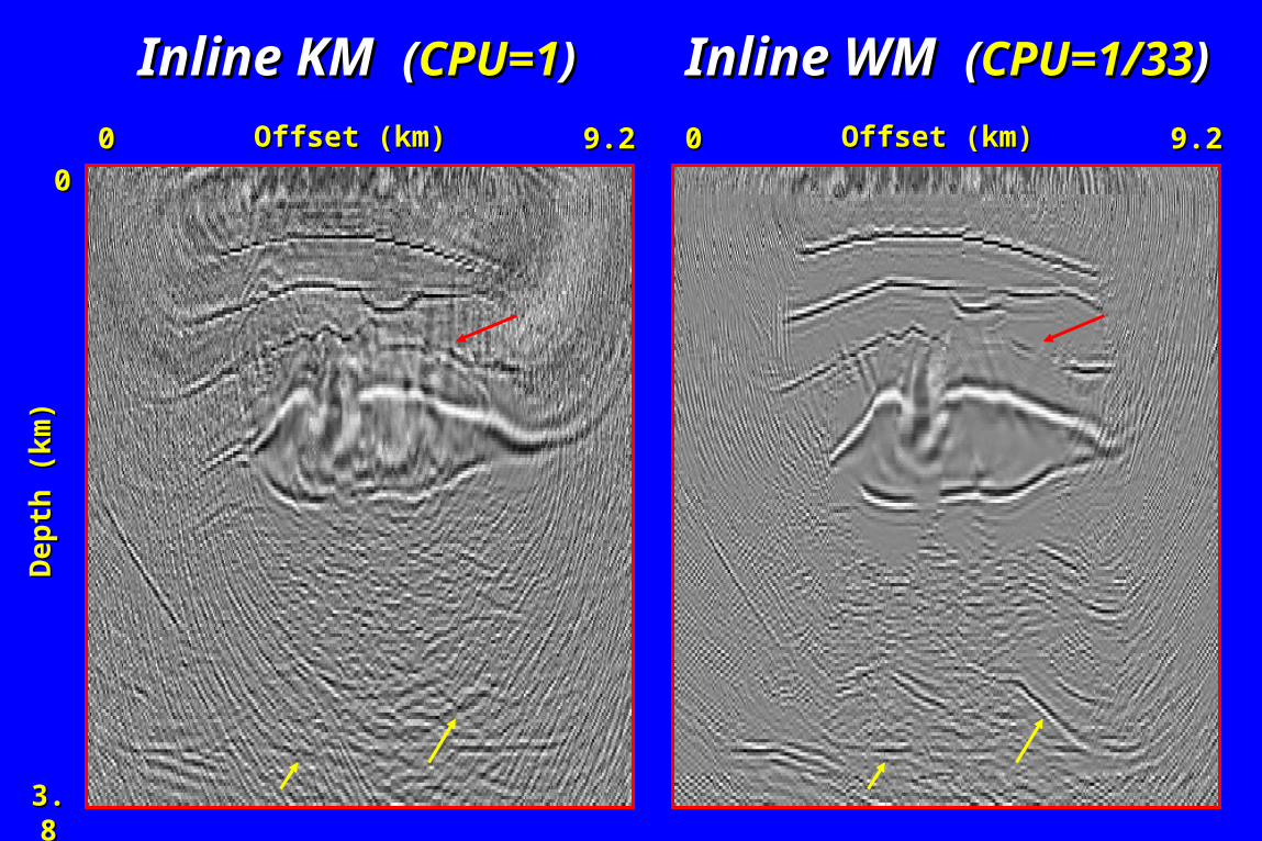
Inline KMInline KM ((CPU=1CPU=1)) Inline WMInline WM ((CPU=1/33CPU=1/33))
Offset (km)Offset (km)00 9.29.2
00
3.83.8
De
pth
(k
m)
De
pth
(k
m)
Offset (km)Offset (km)00 9.29.2

Receiver DistributionReceiver DistributionC
ross
line
(m)
Cro
sslin
e (m
)
44804480
23202320
19201920
19201920 Inline (m)Inline (m)

Inline KMInline KM ((CPU=1CPU=1)) Inline WMInline WM ((CPU=1/170CPU=1/170))
Offset (km)Offset (km)00 9.29.2
00
3.83.8
De
pth
(k
m)
De
pth
(k
m)
Offset (km)Offset (km)00 9.29.2
(subsample)(subsample)
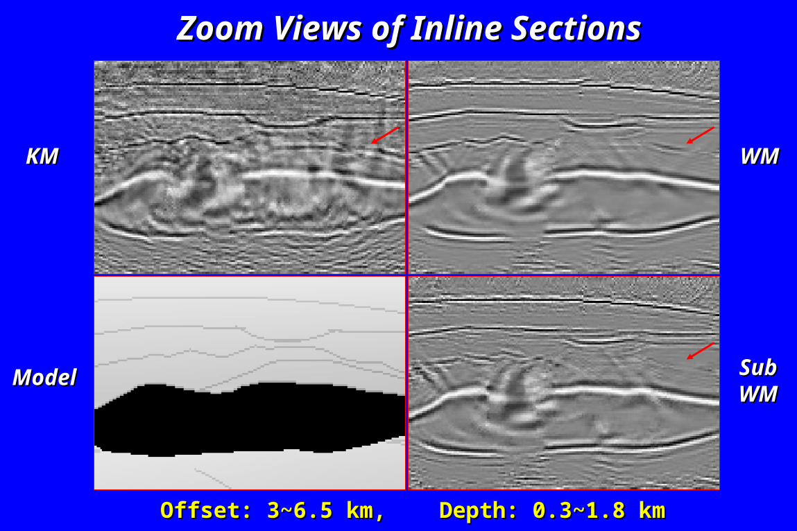
Zoom Views of Inline Sections Zoom Views of Inline Sections
Offset: 3~6.5 km, Depth: 0.3~1.8 kmOffset: 3~6.5 km, Depth: 0.3~1.8 km
WMWM
ModelModel
KM KM
SubSubWMWM

Offset: 1.8~4 km, Depth: 0.6~2.1 kmOffset: 1.8~4 km, Depth: 0.6~2.1 km
WMWM
ModelModel
KM KM
SubSubWMWM
Zoom Views of Crossline Sections Zoom Views of Crossline Sections

Inline: 1.8~7.2 km, Crossline: 0~4 kmInline: 1.8~7.2 km, Crossline: 0~4 km
WMWM
ModelModel
KM KM
SubSubWMWM
Horizontal Slices (Depth=1.4 km) Horizontal Slices (Depth=1.4 km)

OutlineOutline• Problems in 2-D WMProblems in 2-D WM• Objectives of 3-D WM Objectives of 3-D WM Numerical ResultsNumerical Results 3-D Point Scatterer Data3-D Point Scatterer Data 3-D SEG/EAGE Salt Data3-D SEG/EAGE Salt Data 3-D West Texas Field Data3-D West Texas Field Data• ConclusionsConclusions

A Common Shot GatherA Common Shot GatherTrace NumberTrace Number5454 193193
Tim
e (s
ec)
Tim
e (s
ec)
00
3.43.4
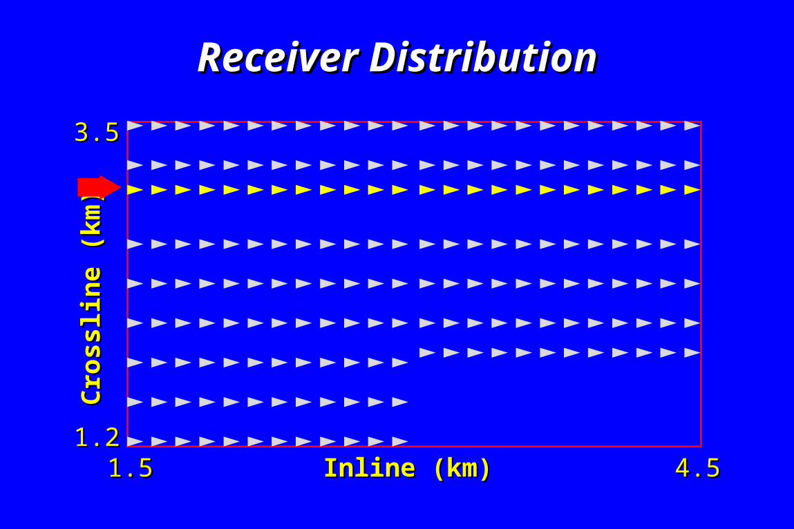
Receiver DistributionReceiver DistributionC
ross
line
(km
)C
ross
line
(km
)
4.54.51.21.2
3.53.5
1.51.5 Inline (km)Inline (km)

Receiver DistributionReceiver DistributionC
ross
line
(km
)C
ross
line
(km
)
4.54.51.21.2
3.53.5
1.51.5 Inline (km)Inline (km)

Inline KM Inline KM ((CPU=1CPU=1)) Inline WMInline WM ((CPU=1/14CPU=1/14))
Offset (km)Offset (km)0.40.4 4.54.5
0.80.8
3.83.8
De
pth
(k
m)
De
pth
(k
m)
Offset (km)Offset (km)0.40.4 4.54.5

Inline KMInline KM ((CPU=1CPU=1)) Inline WMInline WM ((CPU=1/50CPU=1/50))
Offset (km)Offset (km)0.40.4 4.54.5
0.80.8
3.83.8
De
pth
(k
m)
De
pth
(k
m)
Offset (km)Offset (km)0.40.4 4.54.5
(subsample)(subsample)

Crossline KM Crossline KM ((CPU=1CPU=1)) Crossline WMCrossline WM ((CPU=1/14CPU=1/14))
Offset (km)Offset (km)0.30.3 3.53.5
0.80.8
3.33.3
De
pth
(k
m)
De
pth
(k
m)
Offset (km)Offset (km)0.30.3 3.53.5

Crossline KMCrossline KM ((CPU=1CPU=1)) Crossline WMCrossline WM ((CPU=1/50CPU=1/50))(subsample)(subsample)
Offset (km)Offset (km)0.30.3 3.53.5
0.80.8
3.33.3
De
pth
(k
m)
De
pth
(k
m)
Offset (km)Offset (km)0.30.3 3.53.5

Inline: 0~4.6 km, Crossline: 0~3.8Inline: 0~4.6 km, Crossline: 0~3.8
KM (KM (CPU=1CPU=1))
Horizontal Slices (Depth=2.5 km) Horizontal Slices (Depth=2.5 km)
WM (WM (CPU=1/14CPU=1/14)) WM (Sub, WM (Sub, CPU=1/50CPU=1/50))

OutlineOutline
• Problems in 2-D WMProblems in 2-D WM• Objectives of 3-D WM Objectives of 3-D WM • Numerical ResultsNumerical Results ConclusionsConclusions

ConclusionsConclusions
SEG/EAGE Salt DataSEG/EAGE Salt Data• Fewer Migration ArtifactsFewer Migration Artifacts• Better for Complex Salt BoundaryBetter for Complex Salt Boundary• Higher Computational EfficiencyHigher Computational Efficiency
CPUCPU KM: KM: 11 WM: WM: 1/331/33 Subsampled WM: Subsampled WM: 1/1701/170

ConclusionsConclusions
West Texas Field DataWest Texas Field Data• Fewer Migration ArtifactsFewer Migration Artifacts• Similar Image QualitySimilar Image Quality• Higher Computational EfficiencyHigher Computational Efficiency
CPUCPU KM: KM: 11 WM: WM: 1/141/14 Subsampled WM: Subsampled WM: 1/501/50

ConclusionsConclusions
• Trade-off:Trade-off: between Image Quality between Image Quality and CPU Costsand CPU Costs
• Caution:Caution: WM Angle Estimation WM Angle Estimation Sensitive to Recording Geometry Sensitive to Recording Geometry

• More Robust Angle CalculationMore Robust Angle Calculation• Crossing-event CalculationCrossing-event Calculation• 3-D Marine Field Data3-D Marine Field Data• 3-D Iterative Velocity Analysis3-D Iterative Velocity Analysis
Future WorkFuture Work

Real-time Velocity UpdatingReal-time Velocity Updatingfor Target-oriented Migrationfor Target-oriented Migration
Possible ?Possible ?
QuestionQuestion

AcknowledgementsAcknowledgements
I thank UTAM sponsorsI thank UTAM sponsorsfor their financial supportfor their financial support