IEEE TRANSACTIONS ON MAGNETICS, VOL. 31, NO. 3, MAY 1995 226 I

3-D Eddy-Current Computation with a Self-Adaptive Refinement

N. A. Golias, Member, IEEE, and

Abstract-A method for the adaptive computation of 3-D eddycurrent problems is presented. The 3-D eddy-current problem is formulated in terms of the electric intensity ( E for- mulation). Edge elements that impose tangential continuity of the approximation function are employed for the discretization of the problem with the finite element method. An a-posferiori error estimation technique is proposed with the introduction of two error criteria: a) the tangential discontinuity of the mag- netic intensity H , and b) the normal discontinuity of the eddy current density J,. The proposed error estimation technique is employed in a 3-D self-adaptive refinement procedure. Suffi- cient approximation of the skin effect and calculation of the eddy current distribution is obtained with the proposed method. The implementation of the proposed technique in a problem of 3-D eddy-current computation in a multiply connected con- ducting body is discussed.

I. INTRODUCTION DDY CURRENT problems constitute a wide class of E time-varying electromagnetic problems in which the

contribution of the displacement current is considered negligible. In these problems the change of the magnetic flux density gives rise to an electric intensity, which causes the development of eddy currents in conducting materials. In this way energy is diffused in conducting bodies and is transformed into Joule losses.

Eddy currents tend to develop on the outer surfaces of conductors, a phenomenon known as skin effect. The pen- etration depth is a very important parameter in eddy cur- rent phenomena, and expresses the ability of penetration of the electromagnetic field in conducting bodies. The skin effect has a direct relation to frequency. Eddy currents appear mainly in 1-5 depths of penetration. The higher the frequency, the smaller the penetration depth.

The proper operation of many electromagnetic devices depends on the distribution of eddy currents in their con- ducting parts. Therefore, the knowledge of the distribu- tion of eddy currents within conducting bodies is very im- portant and an accurate calculation is often needed. Many methods have been employed for the solution of eddy cur- rent problems [16], [19]. The finite element method has been used extensively during the last decade for the so- lution of 3-D eddy-current problems [1]-[3], [6], 171, [ 181. Of particular interest are the formulations in terms

Manuscript received February 11, 1994; revised September 19, 1994. The authors are with the Department of Electrical and Computer Engi-

neering, Aristotle University of Thessaloniki, Thessaloniki, 54006, Greece. IEEE Log Number 9407360.

Technique T. D. Tsiboukis, Member, IEEE

of a field variable directly. Two such formulations have been proposed for 3-D eddy-current problems, one in terms of the magnetic intensity H, and one in terms of the electric intensity E [8]. The formulation that employs the magnetic intensity H as the primary unknown is valid in conducting material only, so it has to be coupled to an integral equation technique. A sufficient implementation of the so called H formulation with edge elements is pre- sented in [3].

The formulation in terms of the electric intensity E is valid in the whole domain [5]. This allows for a complete formulation with the electric intensity in conducting and non-conducting domains as the primary unknown. Al- though this formulation is particularly useful when the distribution of the electric intensity is required in non- conducting domains, e.g., in air, it may be considered a disadvantage when the primary region of interest is the conducting material. It can be argued that in problems where the main objective is the calculation of the distri- bution of eddy currents in conducting bodies, the distri- bution of the electromagnetic fields outside the conduct- ing material is of no importance, so the discretization of non-conducting material leads to increased computational cost.

The problem of the increased computational cost, due to the discretization of nonconducting regions, as well as the sufficient approximation of the skin effect, can be ad- dressed with the employment of a self-adaptive refine- ment technique. Adaptive techniques offer the optimum solution to a problem with the minimum cost. Several adaptive techniques in 2-D have been developed during the last decade. An efficient computation of 2-D eddy- currents with an adaptive refinement technique, taking into account the skin effect, was presented in [9]. The appli- cation of an adaptive refinement technique has the result of increasing the density of elements in conducting bod- ies, especially near the outer surfaces. Due to the skin effect the eddy current distribution is confined. In this way, a calculation of the eddy current distribution with increased accuracy can be obtained.

It is only recently that several significant contributions have appeared in the area of adaptive refinement in 3-D. The delay, probably due to the difficulty in developing geometrical algorithms for refining 3-D meshes, has been surpassed with the proposal of several techniques [ 111, [ 151, [ 171. Three dimensional refinement algorithms based on the discontinuity of the tangential component of the

0018-9464/95$04.00 0 1995 IEEE

2262 IEEE TRANSACTIONS ON MAGNETICS, VOL. 31, NO. 3, MAY 1995

magnetic intensity H applied in the solution of the mag- netostatic problem were presented in [15], [17]. A for- mulation applied to 3-D scalar problems was presented in [lo], while an implementation of a 3-D adaptive refine- ment algorithm, exploiting the symmetry and comple- mentarity of Maxwell’s equations for error estimation showed very good results [13].

An error estimation technique is proposed in this paper for the automatic self-adaptive solution of 3-D eddy-cur- rent problems. The proposed error estimator is intimately related to the symmetry of Maxwell’s equations and the constitutive laws. The nature of the proposed error esti- mator is easily perceived by considering the Tonti dia- gram for eddy current problems, a convenient way of rep- resenting Maxwell’s equations in diagrammatic form. The proposed error estimation technique consists of two com- ponents. The first one is based on the discontinuity of the tangential component of the magnetic intensity across ele- ment interfaces. The second one is based on the discon- tinuity of the normal component of the eddy current den- sity. The proposed technique is applied to the calculation of the distribution of 3-D eddy-currents in a multiply con- nected conductor.

11. FORMULATION OF THE PROBLEM A . Maxwell Equations

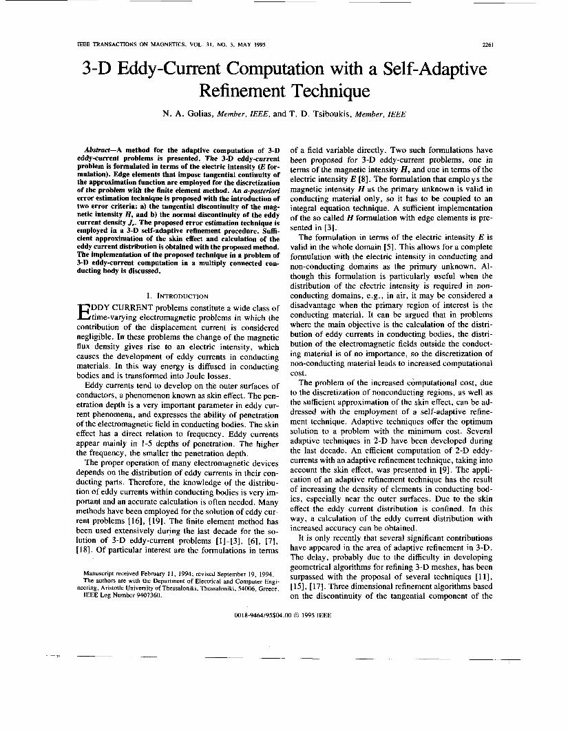
Consider the solution of the eddy current problem in the domain of Fig. 1. Neglecting displacement currents and assuming time harmonic problems, Maxwell’s equa- tions for the eddy current case become

V x E = -jwB (1)

V x H = J, + J, (2)

V * B = O (3) with the constitutive relations

B = p H

Je = uE

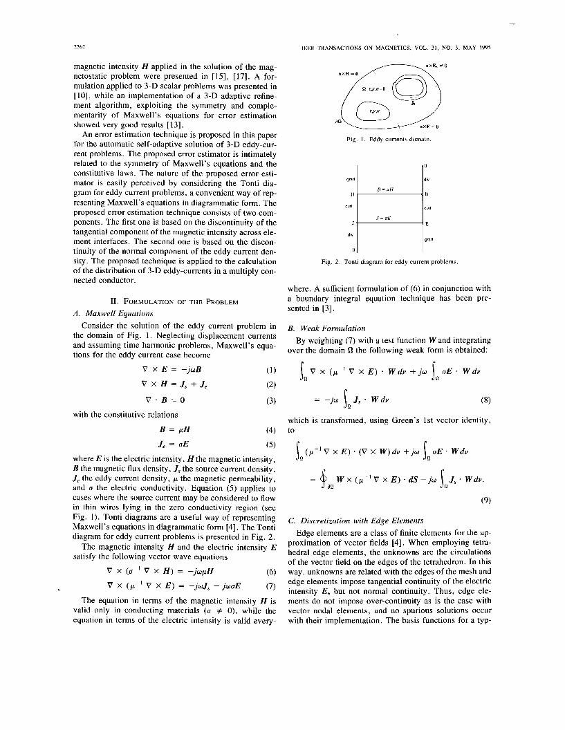
where E is the electric intensity, H the magnetic intensity, B the magnetic flux density, J, the source current density, Je the eddy current density, p the magnetic permeability, and U the electric conductivity. Equation ( 5 ) applies to cases where the source current may be considered to flow in thin wires lying in the zero conductivity region (see Fig. I ) . Tonti diagrams are a useful way of representing Maxwell’s equations in diagrammatic form [4]. The Tonti diagram for eddy current problems is presented in Fig. 2.

The magnetic intensity H and the electric intensity E satisfy the following vector wave equations

(6)

(7) The equation in terms of the magnetic intensity H is

valid only in conducting materials (a # 0), while the equation in terms of the electric intensity is valid every-

v x ( U - ’ v x H ) = -jwpH

V x ( p - I V x E ) = -jwJ, - jwuE

- nxE, # O

: = 0

Fig. 1. Eddy currents domain.

curl

J = a E

div cur:HE grad

Fig. 2. Tonti diagram for eddy current problems.

where. A sufficient formulation of (6) in conjunction with a boundary integral equation technique has been pre- sented in [3].

B. Weak Formulation

over the domain D the following weak form is obtained: By weighting (7) with a test function Wand integrating

s , V x ( p - l V x E ) * W d u + jw

= -jw J, W d u sa which is transformed, using Green’s 1st vector identity, to

s a ( p - I V x E ) * ( V x W ) d u + j w sa u E - Wdu

P I-

= $ W x ( p - l V X E ) . d S - j w aa

(9)

C. Discretization with Edge Elements Edge elements are a class of finite elements for the ap-

proximation of vector fields [4]. When employing tetra- hedral edge elements, the unknowns are the circulations of the vector field on the edges of the tetrahedron. In this way, unknowns are related with the edges of the mesh and edge elements impose tangential continuity of the electric intensity E , but not normal continuity. Thus, edge ele- ments do not impose over-continuity as is the case with vector nodal elements, and no spurious solutions occur with their implementation. The basis functions for a typ-

GOLIAS AND TSIBOUKIS: 3-D EDDY-CURRENT COMPUTATION 2263

ical edge e = { i , j } connectiiig vertices i and j of a tetra- hedral element, are given by

where Ci (i = 1, 2, 3, 4) are the simplex coordinates or barycentric functions of the corresponding nodes.

The electric intensity in a tetrahedron is approximated as

6

E = EeW, (1 1) e = I

where the coefficients E, are the circulations of the elec- tric intensity along the edges of the tetrahedron.

If the edge element shape functions are used as the weighting function W in (9), it is discretized as

{[SI +ju[Tll[Xl = [4 (12) where [SI, [TI and [b] are matrices with elements

S- = ( p - ' V X Wi) (V X Wj)dv (13) r J Q s

P

r

Solution of (12) is accomplished with an iterative pre- conditioned conjugate gradient technique exploiting sym- metry and sparsity of the finite element matrices [14].

111. ERROR ESTIMATION The magnetic induction is calculated as B = V x

El( -ju) in terms of the electric intensity E, as is shown in the Tonti diagram for eddy currents (Fig. 2). The re- maining pair of electromagnetic quantities, the magnetic intensity H, and the eddy current density J, are calculated by traversing the horizontal bars of the Tonti diagram, thus making use of the constitutive laws H = p-IB and J , = UE respectively. The magnetic intensity and the eddy current density, calculated in this way, do not present the right continuity conditions across interfaces. Actually, the magnetic intensity H presents tangential discontinuity, while the eddy current density J, presents normal discon- tinuity across element interfaces.

In this context two new error estimators for eddy cur- rent problems are proposed: a) the tangential discontinu- ity of the magnetic intensity H, and b) the normal discon- tinuity of the eddy current density J,. Consider two tetrahedra (e) and (f) and their common face (ABC). Let H(') and H ( f ) denote the magnetic intensity in tetrahedra (e) and (f) respectively. The error estimator of the mag- netic intensity H of face (ABC) is defined by the follow- ing quantity:

EZ$Bc) = I no x (H") - @')I2 dS. (16) S(ABC)

Let J f ) and J k f ' denote the eddy current density in tet- rahedra (e) and (f) respectively. The error estimator of the eddy current density J, of face (ABC) is defined as:

EZ&) = 1 I(JF' - J L f ' ) * nOl2 dS. (17) &ABC)

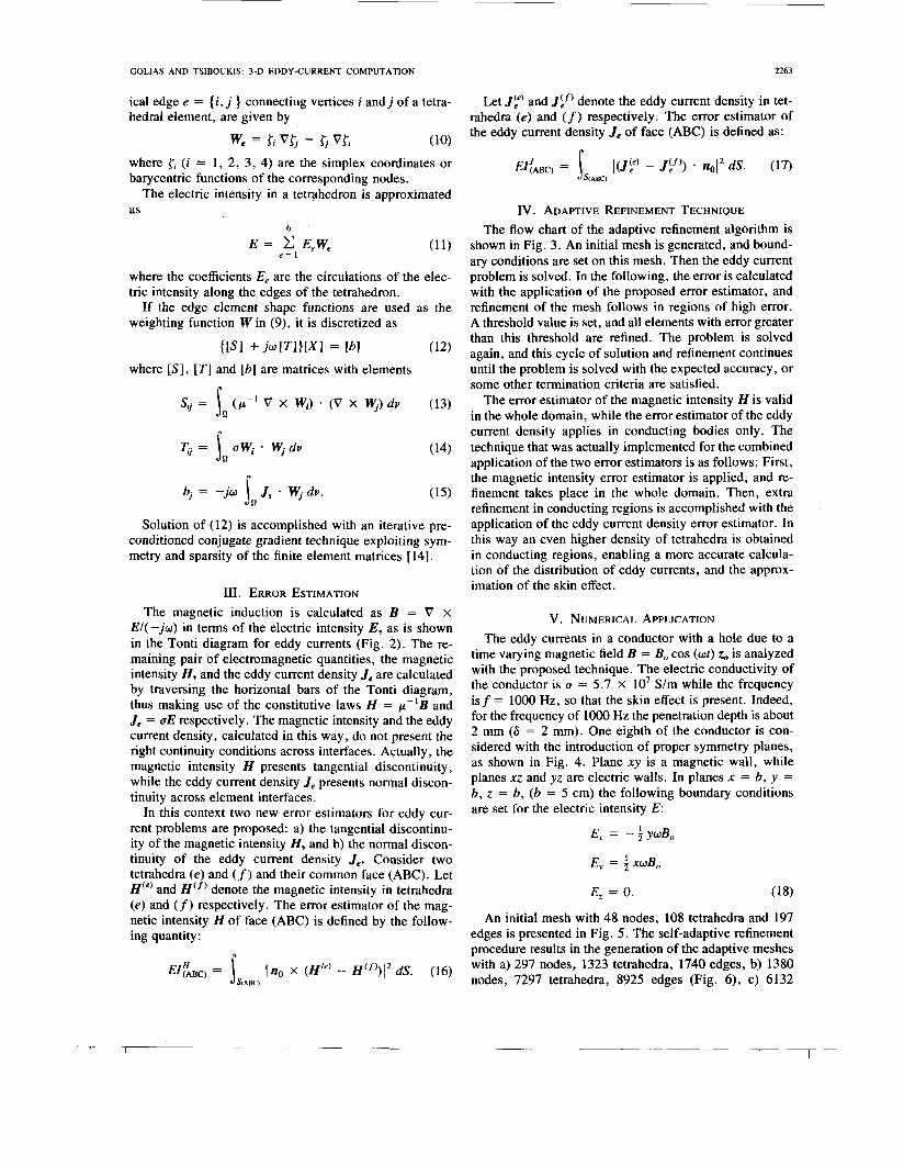
IV. ADAPTIVE REFINEMENT TECHNIQUE The flow chart of the adaptive refinement algorithm is

shown in Fig. 3. An initial mesh is generated, and bound- ary conditions are set on this mesh. Then the eddy current problem is solved. In the following, the error is calculated with the application of the proposed error estimator, and refinement of the mesh follows in regions of high error. A threshold value is set, and all elements with error greater than this threshold are refined. The problem is solved again, and this cycle of solution and refinement continues until the problem is solved with the expected accuracy, or some other termination criteria are satisfied.

The error estimator of the magnetic intensity H i s valid in the whole domain, while the error estimator of the eddy current density applies in conducting bodies only. The technique that was actually implemented for the combined application of the two error estimators is as follows: First, the magnetic intensity error estimator is applied, and re- finement takes place in the whole domain. Then, extra refinement in conducting regions is accomplished with the application of the eddy current density error estimator. In this way an even higher density of tetrahedra is obtained in conducting regions, enabling a more accurate calcula- tion of the distribution of eddy currents, and the approx- imation of the skin effect.

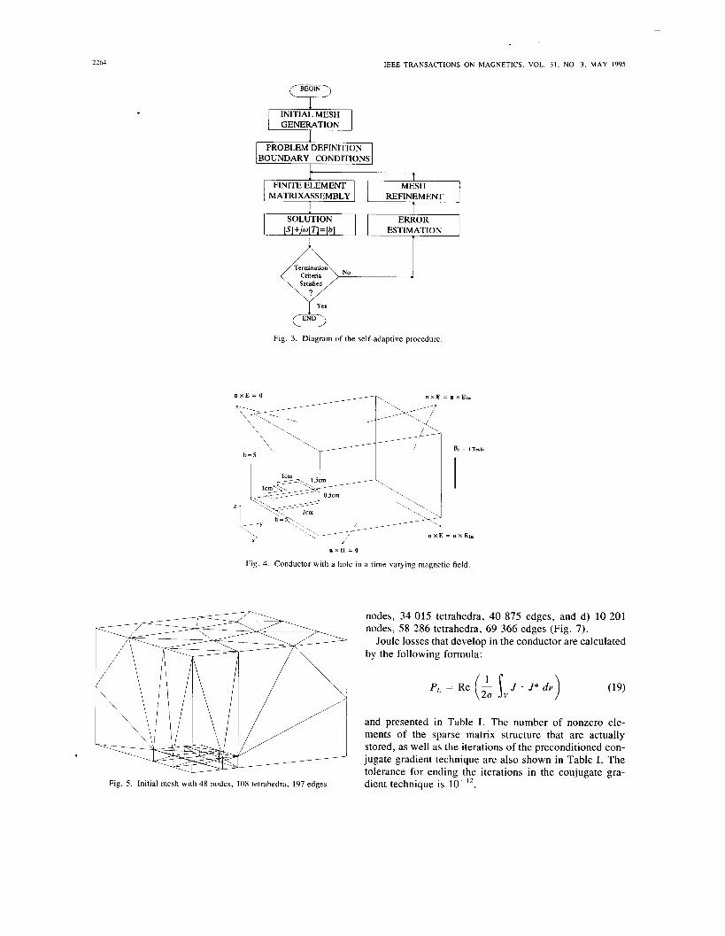
V. NUMERICAL APPLICATION The eddy currents in a conductor with a hole due to a

time varying magnetic field B = Bo cos (ut) z, is analyzed with the proposed technique. The electric conductivity of the conductor is U = 5.7 X lo7 S/m while the frequency isf = 1000 Hz, so that the skin effect is present. Indeed, for the frequency of IO00 Hz the penetration depth is about 2 mm (6 = 2 mm). One eighth of the conductor is con- sidered with the introduction of proper symmetry planes, as shown in Fig. 4. Plane x y is a magnetic wall, while planes xz and yz are electric walls. In planes x = b, y = b, z = b, ( b = 5 cm) the following boundary conditions are set for the electric intensity E:

E = -1. u B x 2 Y U

Ey = i x u B ,

E, = 0. (18)

An initial mesh with 48 nodes, 108 tetrahedra and 197 edges is presented in Fig. 5 . The self-adaptive refinement procedure results in the generation of the adaptive meshes with a) 297 nodes, 1323 tetrahedra, 1740 edges, b) 1380 nodes, 7297 tetrahedra, 8925 edges (Fig. 6), c) 6132

2264

FINITE ELEMENT MATRIXASSEMBLY

SOLUTION [SI +jw[T) = [b]

I

IEEE TRANSACTIONS ON MAGNETICS, VOL. 31. NO. 3, MAY 1995

MESH REFINEMENT

ERROR ESTIMATION

T

Satisfied

& Fig. 3 . Diagram of the self-adaptive procedure.

n x E = O n x E = n x Ei.

U X H = O

Fig. 4. Conductor with a hole in a time-varying magnetic field.

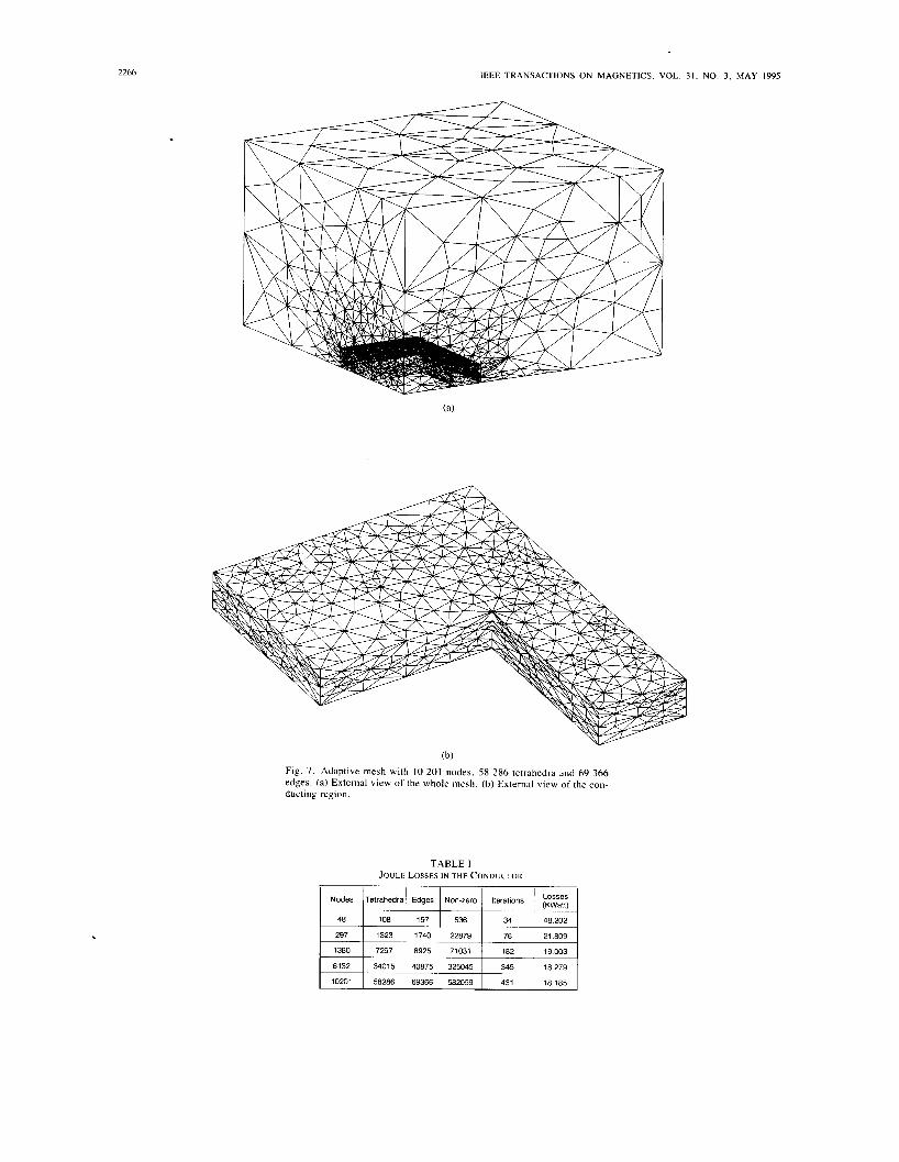
nodes, 34 015 tetrahedra, 40 875 edges, and d) 10 201 nodes, 58 286 tetrahedra, 69 366 edges (Fig. 7).

Joule losses that develop in the conductor are calculated by the following formula:

PL = Re (L 20 v J J* dv) (19)

and presented in Table I . The number of nonzero ele- ments of the sparse matrix structure that are actually stored, as well as the iterations of the preconditioned con- jugate gradient technique are also shown in Table I. The tolerance for ending the iterations in the conjugate gra- dient technique is Fig. 5 . Initial mesh with 4 8 nodes, 108 tetrahedra, 197 edges.

GOLIAS AND TSIBOUKIS: 3-D EDDY-CURRENT COMPUTATION 2265

(b)

Fig. 6. Adaptive mesh with 1380 nodes, 7297 tetrahedra and 8925 edges. (a) Extemal view of the whole mesh. (b) Extemal view of the conducting region.

It is observed that the iterative procedure has a very good convergence since 40 875 equations are solved with 345 iterations, and 69 366 equations are solved with 431 iterations. An adaptive mesh better approaches the correct distribution of the electromagnetic field, which results in a well-conditioned system of equations. In addition, the condition of the set of equations depends on the quality of the tetrahedral elements. The tetrahedral elements,

produced with the refinement algorithm based on Delau- nay transformations, are of very high quality (nearly equi- lateral) [ 1 11. In this way the obtained system of equations is well conditioned, and the application of the precondi- tioned conjugate gradient technique results in fast con- vergence.

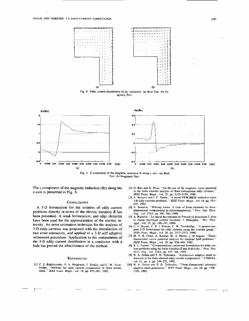
The eddy current distribution in the conducting body is presented in Fig. 8, where the skin effect can be observed.

2266 IEEE TRANSACTIONS ON MAGNETICS, VOL. 31, NO. 3, MAY 1995

(b) Fig. 7. Adaptive mesh with IO 201 nodes, 58 286 tetrahedra and 69 366 edges. (a) External view of the whole mesh. (b) External view of the con- ducting region.

TABLE I JOULE LOSSES IN THE CONDUCTOR

GOLIAS AND TSIBOUKIS: 3-D EDDY-CURRENT COMPUTATION

2 -

1.6

1 -

0.6

-0.6

2267

0.6 -

- 0.4 -

0.2 -

- 0

0 1 -0.2 -

-0.4

Fig. 8. Eddy current distribution in the conductor. (a) Real Part. (b) Im- aginary Part.

The z-component of the magnetic induction (Bz) along the x-axis is presented in Fig. 9.

CONCLUSIONS A 3-D formulation for the solution of eddy current

problems directly in terms of the electric intensity E has been presented. A weak formulation, and edge elements have been used for the approximation of the electric in- tensity. An error estimation technique for the analysis of 3-D eddy-currents was proposed with the introduction of two error estimators, and applied in a 3-D self adaptive refinement procedure. Application to the computation of the 3-D eddy-current distribution in a conductor with a hole has proved the effectiveness of the method.

REFERENCES [ I ] C. S. Biddlecombe, E. A. Heighway, J. Simkin, and C. W. Trow-

bridge, “Methods for eddy current computation in three dimen- sions,” IEEE Trans. Magn. , vol. 18, pp. 492-497, 1982.

121 0. Biro and K. Preis, “On the use of the magnetic vector potential in the finite element analysis of three-dimensional eddy currents,” IEEE Trans. Magn., vol. 25, pp. 3145-3159, 1989.

[3] A. Bossavit and J . C. Verite, “A mixed FEM-BIEM method to solve 3-Deddy-currents problems,” IEEE Trans. Magn. , vol. 18, pp. 431- 435, 1982.

141 A. Bossavit, “Whitney forms: A class of finite elements for three- dimensional computations in electromagnetism,” Proc. Inst. Elect. Eng. , vol. 135A, pp. 493-500, 1988.

[5] A. Bossavit, “Le calcul des courants de Foucalt en dimension 3, avec le champ electrique comme inconnue. I: Principles,” Rev. Phys. Appl . , vol. 25, pp. 189-197, 1990.

[6] C. F. Bryant, C. R. I. Emson, C. W. Trowbridge, “A general pur- pose 3-D formulation for eddy currents using the Lorentz gauge,” IEEE Trans. Magn., vol. 26, pp. 2373-2375, 1990.

[7] M. V. K. Chari, A. Konrad, M. A. Palmo, J. D’Angelo, “Three- dimensional vector potential analysis for machine field problems,” IEEE Trans. Magn., vol. 18, pp. 436-446, 1982.

[8] R. L. Ferrari, “Complementary variational formulation for eddy-cur- rent problems using the Field variables E and H directly,” Proc. Insr. E l m . Eng. , vol. 132A. pp. 157-164, 1985.

[9] N. A. Golias and T. D. Tsiboukis, “A-posteriori adaptive mesh re- finement in the finite element eddy current computation,” COMPEL, vol. 11, no. 1, pp. 249-252, 1992.

[ IO] N. A. Golias and T. D. Tsiboukis, “Three-dimensional automatic adaptive mesh generation,” IEEE Trans. Magn. , vol. 28, pp. 1700- 1703, 1992.

2268 IEEE TRANSACTIONS ON MAGNETICS. VOL. 31, NO. 3, MAY 1995

[ I I] N. A. Golias and T. D. Tsiboukis, “An approach to refining three- dimensional tetrahedral meshes bases on Delaunay transformations,” 1/11. J . Nurn. Meth. Eng. , vol. 37, pp. 793-812, 1994.

[I21 N. A. Golias and T. D. Tsiboukis, “Automatic finite element anal- ysis: Application to the shielding by a spherical shell,” Arch. Elekrr.,

[I31 N. A. Golias. T. D. Tsiboukis, and A. Bossavit, “Constitutive in- consistency: rigorous solution of Maxwell equations based on a com- plementary approach,” IEEE Trans. Magn. , Sept. 1994.

[ 141 D. S . Kershaw, “The incomplete Cholesky-conjugate gradient method for the iterative solution of systems of linear equations,” J . Comp.

[I51 H. Kim, S. Hong, K. Choi. H . Jung, and S. Hahn, “A three dimen- sional adaptive finite element method for magnetostatic problems,’’ IEEE Trans. Magn . . vol. 27, pp. 4081-4084, 1991.

[ 161 E. E. Kriezis, T. D. Tsiboukis, S. M. Panas. and J. A. Tegopoulos, “Eddy currents: Theory and applications.” IEEE Proc . , vol. 80, pp.

1171 T. W . Nehl and D. A. Field, “Adaptive refinement of first order tetrahedral meshes for magnetostatics using local Delaunay subdivi- sions,” IEEE Trans. Magn. , vol. 27, pp. 4193-4196, 1991.

[ 181 D. Rodger, “ Finite-element method for calculating power frequency 3-dimensional electromagnetic field distributions,” Proc. Inst. Elect. Eng . , vol. 130A. pp. 233-238, 1983.

(191 G . A. Tegopoulos and E. E. Kriezis, Eddy Currents in Linear Con- ducting Media. New York: Elsevier, 1985.

vol. 77, pp. 85-93, 1994.

Phvs. , vol. 26, pp. 43-65, 1978.

1556-1589, 1992.

Nikolaos A. Golias (S’91-M’93) was born in Veria, Greece, on April 29, 1966. He received the Dipl. Eng. degree in electrical engineering from the Aristotle University of Thessaloniki, Greece in 1989, and the Ph.D. degree from the same institution in 1993.

Since 1989 he has been a research assistant at the Department of Elec- trical Engineering at the University of Thessaloniki. His research activities include the application of the finite element method to the field solution of various engineering problems, and the development of adaptive techniques in 2-3-dimensions.

Dr. Golias is a member of the Technical Chamber of Greece, and a mem- ber of IEEE.

Theodoros D. Tsiboukis (S’79-M’91) was born in Larissa, Greece. on February 25, 1948. He received the Dipl. Eng. degree from the National Technical University of Athens, Athens. Greece, in 1971, and the Ph.D. degree from the Aristotle University of Thessaloniki, Thessaloniki. Greece, in 1981.

Since 1981 he has been working at the Department of Electrical Engi- neering of the Aristotle University of Thessaloniki. where he is now an Associate Professor. He is the author of several books and papers. His research activities include electromagnetic field analysis by energy meth- ods with emphasis to the development of special finite element techniques to the field solution of various engineering applications.

Dr. Tsiboukis is a member of the Technical Chamber of Greece, and a member of IEEE.