2s nuclear instruments 8 methods in phvsics … · nuclear instruments and methods in physics...
TRANSCRIPT
2s . __
t!z
+j_:
EL..FXVIER
Nuclear Instruments and Methods in Physics Research A 373 (1996) 227-260 NUCLEAR INSTRUMENTS
8 METHODS IN PHVSICS RESEARCH
Sectlon A
Track finding and fitting in the HI Forward Track Detector
S. Burke”‘*, R.C.W. Hendersona, S.J. Maxfieldb, J.V. Morris”, G.D. Patelb, D.P.C. Sankey”, 1.0. Skillicomd
“hncasrer Universip, Lancaster LA I 3YB. UK hUniversity of Liverpool, Liverpool L69 3BX, UK
‘Ruthetford Appleton Laboratory, Didcot. Oxon.. 0x11 OQX, UK ‘Universir)! of Glasgow. Glasgow Cl2 SQQ. UK
Received 30 June 1995
Abstract
The tracking environment in the HI Forward Track Detector, where the hit multiplicity from proton fragments is high, is
particularly hostile. The techniques and software which have been developed for pattern recognition and Kalman fitting of
charged particle tracks in this region are described in detail.
1. Introduction
The Forward Track Detector (FTD) is part of the HI detector used at the HERA accelerator to study high
energy electron-proton collisions. This paper describes the software used for the pattern recognition and fitting of
tracks measured by the Forward Tracker. To set the framework and to motivate the design of the FTD, Section
1 discusses the HERA accelerator and its physics goals, and outlines the construction of the Hl detector. Section 2
describes the hardware of the FTD. The techniques used to
find the hits in the drift chamber data are presented in Section 3, and calibration and monitoring procedures are
described in Section 4. Sections 5 and 6 discuss the algorithms developed for finding line segments in the drift chambers and the methods used for joining the segments to form tracks. A Kalman filter technique is used for de-
termining track parameters; this is described in Section 7. The method used to align the Forward Tracker is outlined
in Section 8. Details of the performance of the software and the relation between this performance and that of the
hardware are given in Section 9. Section 10 summarises the conclusions.
1.1. The HERA accelerator
The HERA accelerator has been constructed to investi- gate lepton-quark interactions at high energy by colliding 30 GeV electrons with 820 GeV protons. The experimental programme at HERA includes searches for new physics,
* Corresponding author.
such as massive new bosons, super-symmetric particles, lepton and quark substructure. and heavy leptons. It permits measurement of the proton structure functions up
to values of Q’ that are two orders of magnitude greater than previous experiments and down to values of xs, two
orders of magnitude lower [I].
1.2. The HI detector
The kinematics of HERA collisions lead to an asymmet-
ric detector design [2]. The centre of mass of the collision
moves in the proton direction, and consequently any collision products are boosted along this direction. The HI
detector is designed to provide a smooth and homogeneous response from small forward angles (with respect to the proton direction) through to backward angles. The mea-
surement of charged tracks at small angles requires a Forward Tracker.
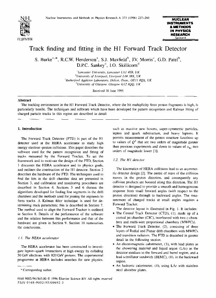
The detector layout is illustrated in Fig. I. It includes:
The Central Track Detector (CTD), (I), made up of a central jet chamber (CJC), interleaved with two z-cham-
bers and multi-wire proportional chambers (MWPCs). The Forward Track Detector, (2), consisting of three
layers of Radial and Planar drift chambers with MWPCs and transition radiators. The FTD is described in greater detail in the following section. An electromagnetic calorimeter, (3), with lead plates as the showering material and liquid argon (LAr} as the detector medium in the forward and barrel region, and a lead scintillator sandwich (BEMC), (8), in the backward region. An hadronic calorimeter, (4), using LAr with stainless steel absorber plates.
016%9002/96/$15.00 0 1996 Elsevier Science B.V. All rights reserved
SSDl 0168-9002(95)00692-3
228
Y
electron detector
Fig. 1. Schematic y-z view of the Hl detector. Also included is the luminosity monitor, situated downstream in the electron direction (not
to scale). The nominal interaction point is marked by . . See text for key.
A superconducting solenoid giving a field of about 1.2 T, (5), outside the hadronic calorimeter. An outer shell of iron plates to contain the return
magnetic flux, (6). The iron is interleaved with plastic
streamer tubes to act as a tail-catcher for the hadronjc calorimeter and as a muon detector and tracker.
Additional muon detection, provided by three layers of muon chambers in the barrel and forward region. along with a forward muon spectrometer, which consists of a
magnetised iron toroid, (7) and six layers of drift
chambers, ( IO). A plug calorimeter, (9), to detect hadronic energy at small angles (>0.7”) built as a copper and silicon
sandwich. A time-of-flight scintillator, (I I), to veto events not
originating at the vertex. A luminosity monitor, ( 12).
1.2. I. The HI coordinate system The Hl coordinate system is right-handed and is defined
with respect to the Central Tracker. The nominal positive z-axis is in the proton direction with the y-axis vertical; 0 and $ represent the polar and azimuthal angles respective- ly, and in this paper R denotes the radial coordinate in the X, v plane. The origin of the coordinate system is defined to be at the centre of the CTD (the nominal e-p interaction
point).
2. Overview of the Forward Track Detector
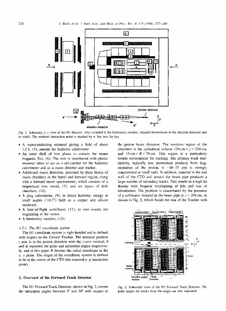
The Hl Forward Track Detector, shown in Fig. 2, covers the laboratory angles between 5” and 30” with respect to
the proton beam direction. The sensitive region of the chambers is the cylindrical volume I34 cm < z < 254 cm.
and 1.5 cm <R < 79 cm. This region is a particularly hostile environment for tracking. The primary track mul-
tiplicity. typically low momentum products from frag-
mentation of the proton, is -IO- I5 and is strongly concentrated at small radii. In addition, material in the end
wall of the CTD and around the beam pipe produces a large number of secondary tracks. This results in a high hit density with frequent overlapping of hits and loss of information The problem is exacerbated by the presence
of a collimator situated in the beam pipe at z = 204 cm, as shown in Fig. 2, which floods the rear of the Tracker with
Fig. 2. Schematic view of the Hl Forward Track Detector. The polar angles for tracks from the origin are also indicated.

S. Burke et al. I Nucl. Instr. and Merh. in Phys. Res. A 373 (1996) 227-260 229
additional secondary tracks, doubling the number of hits in
that region. Consequently 80% of all tracks and 60% of
those with momentum, p, >O.S GeV/c which penetrate the
Forward Tracker are secondaries. The design obiectives for the Forward Tracker were [3]:
momentum resolution for tracks (p > IO GeV/c) con- strained to the primary vertex of (lip’ - 0.003 (GeV/
c)-‘, angular resolution of <l mrad,
efficient track pattern recognition,
efficient electron identification, with pion contamination below 10% for particle momenta up to 60 GeV/c.
a fast ray trigger (provided by the MWPCs). The last two points are not discussed in this paper [4]. These objectives were subject to the overall constraint of
introducing the minimum amount of material before the calorimeter [ 51.
The detector is realised as three identical sub-units, known as Supermodules, numbered from 0 to 2 with
increasing Z. Each Supermodule, when seen from the
direction of the incoming proton, consists firstly of three
layers of Planar drift chambers, oriented at 0”, $60” and -60” to the vertical. followed by an MWPC, then transi-
tion radiator material, and finally a Radial drift chamber.
As each part of the Supermodule uses a different gas mixture (Ar/C,H, for the Planar chambers and MWPCs, He/CO? for the transition radiator and Ar/C>H, or Xe/ He/C2H, for the Radial chambers) each Supermodule is
housed in a correspondingly segmented gas tank. The tank also forms the mechanical frame for the FTD, supporting it on rails inside the liquid argon cryostat.
2.1. The Radial chambers
Each of the three Radial drift chambers, situated approx- imately 1.7, 2.1 and 2.5 m from the interaction point,
consists of 48 wedge-shaped segments, each segment subtending 7.5” in 4 [6]. The layout of a Radial chamber is shown in Fig. 3. Each segment contains a plane of
twelve sense wires, spaced apart by I cm along the beam direction, and eleven intermediate field wires, strung between a central hub and the outer shell. The sense wires
are alternately staggered by 288 km out of the true radial wire-plane, to permit resolution of the left/right track
ambiguity. The radial wire geometry described above was dictated
by the following considerations: the available space is filled most efficiently, providing
drift cells of smaller size at smaller radius, where track illumination is higher; multi-track pattern recognition is optimised, because a track makes hits which have a linear dependence of 4 on i: the drift time measurement is an accurate determination of the track sagitta in the R-4 plane (orthogonal to the magnetic field), so that optimum particle momentum precision may be achieved.
Fig. 3. Perspective schematic of a Radial chamber.
The sense wires are 50 pm diameter Stablohm 800. The simultaneous requirements of having the chamber operate
in a proportional mode for energy loss measurements and
of demanding total ionisation collection for efficient
transition radiation (X-ray) detection dictate the choice of relatively large diameter sense wires. At the hub each
sense wire is connected to its partner 105” away in 4; each
such wire-pair is read out at the outer circumference of the chamber and the radial coordinate reconstructed from charge division along the wire-pair.
2.2. The Planar chambers
The Planar system consists of three identical modules situated approximately 1.4, 1.8, and 2.2 m from the
interaction point [2]. Each module consists of 12 planes of wires perpendicular to the z-axis. Each plane contains 32 parallel sense wires of diameter 40 km with a spacing of 5.7 cm. These wires form a sensitive disc of radius 79 cm
perpendicular to the beam direction. There is a concentric I5 cm radius hole in the disc for the beam pipe, and wires that would otherwise cross this are split into two separate parts. Within a module the first four planes have wires which are aligned vertically, the next four at 60” and the final four at -60” to the vertical. These three sets of planes are referred to as the X, U, and V orientations respectively, Fig. 4.
An orientation consists of 32 cells each containing four

Three orientations each Three orientations in each module
z- axis ________
a) b)
Fig. 4. Details of Planar orientations. (a) A full Planar module comprising three orientations and (b) the contiguration of the X, U. V
orientations within the Forward Tracker
sense and ten grid wires. The sense wires are separated by
0.6 cm along the z axis and staggered by 300 pm either side of the cell centre with a maximum drift distance of
approximately 2.8 cm, see Fig. 5. The three orientations of a Planar chamber module allow
the reconstruction of a track segment that is well defined in both the radial and 4 directions and thus the Planar
chambers complement the Radial chambers that measure
accurately in 4 only.
3. Hit finding in the drift chambers
The sense wires in the Forward Tracker are read out
using 104MHz 8 bit nonlinear Flash Analogue-to-Digital
Converters (FADCs) giving a history of the chamber pulses in time-slices of 9.6 ns. In the Radial chambers both
ends of each wire-pair are instrumented, whereas in the Planar chambers the wires are instrumented at one end
only. When an event is triggered this history is scanned for
regions containing significant raw data [2]. These regions
together with a number of leading time-slices are then
transferred to the next stage of the data acquisition, the QT analysis. This analysis performs a ‘hit’ search on these
data, and for each hit found, corresponding to the ionisa-
tion left behind by a charged particle passing through the
detector, a charge (Q) and time (t) are determined. The QT analysis techniques for the Radial and Planar
chambers are described separately below.
Detail of a Single cell Grid wires not shown
Fig. 5. Details of Planar cells.
S. Burke ef al. i Nucl. Insir. and Meth. in Phys. Rex. A 373 (1996) 227-260 231
3.1. Radial QT
The raw data are linearised, a pedestal level is de-
termined and a search is then made for hits in each region containing significant data. Having found a hit, a time and charge are determined for each end of the wire-pair ( + , -) separately. A single time for the hit is then calculated by
taking a weighted mean of the two times:
f = (Q+t+ + Q_f_)l(Q+ + Q_) (1)
Using a mean weighted by the charge reduces the
influence of the degraded precision of the time calculated at the end of the wire-pair with the smaller pulse. Both
charges are written out, allowing the later determination of the coordinate along the wire-pair by means of charge division. These steps are described in more detail below.
3.1.1. Hit search The disposition of sense and field wires in the Radial
chambers means that the charge arriving from a track
through the cell, even for one at normal incidence, is
spread over a period of time corresponding to 5 mm drift distance (the different geometry in the Planar cell results in
the corresponding spread being over 1 mm). The Radial
QT therefore uses a first electron method to avoid prob- lems with anisochronicity. along with a strict requirement
on the trailing edge of the pulse to avoid problems with resolved structure in an otherwise clean single hit.
A hit is defined as two or more time-slices above a threshold in the weighted difference of samples (weighted DOS), possibly with intervening time-slices below thres-
hold, followed by at least two time-slices where the
weighted difference of samples is negative, without inter-
vening time-slices above threshold.
The difference of samples (DOS) is defined as [7]:
DOS,(n) = FADC,(n) - FADC,(n - I). (2)
where FADC,(n), the pulse height, is the linearised content of the nth time-slice from end i (2) of the wire-pair,
weighted DOS, W(n). is then defined as the product:
W(n) = c (FADC,(n) - P, -A) X c DOS,(n), I=+- ,=+-
The
(3)
where the pedestal level, P,, is calculated from the flat
region of data at the beginning of the sample and A defines
an arbitrary offset from this pedestal level which allows tuning of the detection efficiency for small hits. An initial estimate of the time of the hit at each end of the wire-pair is defined as the start of the time-slice of the first maximum in 2, _ + DOS,(n) in the data above threshold in
W(n). This method of locating hits has advantages compared to
conventional techniques, such as the simple threshold cut employed by the scanner, or derivatives such as a threshold
cut in DOS, which do not cope well with a non-uniform
background:
using the combined information from both ends of the wire-pair, namely the total charge of the hit, makes the hit search insensitive to the effects of charge division along the wire-pair length (this length is sufficiently
small that propagation delays along the wire-pair may be
neglected at this stage);
using the pulse height and DOS simultaneously reduces the sensitivity to vagaries in the rise time of the pulse.
Overall W(n) forms a strong signal for all but the smallest pulses but is relatively insensitive to an oscillat-
ing or gently rising baseline; combining the information from both ends of the wire-
pair reduces the sensitivity to electronic pickup, which
tends to be out of phase at either end of the wire-pair; W(n) is also sensitive to any further pulses that may be behind the initial detected pulse.
3.12. Time determination For each hit found a time is calculated separately for
each end of the wire-pair using a first electron timing
method. The local DOS maximum within two time-slices
of the initial estimate of the hit time defined above is found
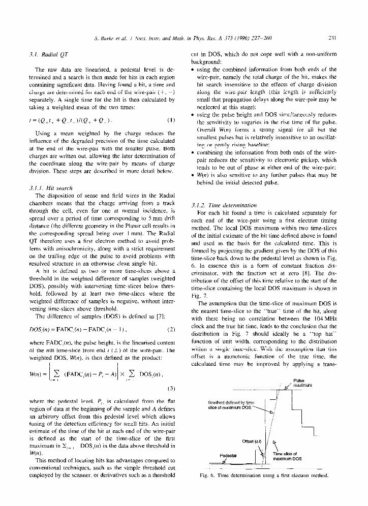
and used as the basis for the calculated time. This is formed by projecting the gradient given by the DOS of this time-slice back down to the pedestal level as shown in Fig. 6. In essence this is a form of constant fraction dis- criminator, with the fraction set at zero [8]. The dis-
tribution of the offset of this time relative to the start of the time-slice containing the local DOS maximum is shown in
Fig. 7.
The assumption that the time-slice of maximum DOS is
the nearest time-slice to the “true” time of the hit, along
with there being no correlation between the 104 MHz clock and the true hit time, leads to the conclusion that the
distribution in Fig. 7 should ideally be a “top hat”
function of unit width, corresponding to the distribution within a single time-slice. With the assumption that this offset is a monotonic function of the true time. the
calculated time may be improved by applying a trans-
Gradient defined by time slice of maximum DOS
!: '1 Offset i I$
Fig. 6. Time determination using a first electron method
232 S. Burke et al. I Nucl. Instr. and Mrth. in Phys. Res. A 37.1 (1996) 127-260
0.03-
0.02 -
0.01- \
0.00 -2.5 -2.0 -1.5 -1 .o -0.5 0.0 0.5
Offset (FADC time slices)
Fig. 7. Distribution of the leading edge intercept with the base
line. relative to the start of the time-slice of maximum DOS.
formation to the observed offset such that the resultant
distribution does have the desired “top hat” shape [9].
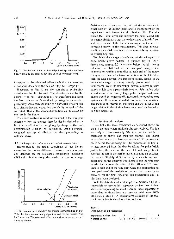
Illustrated in Fig. 8 are the cumulative probability
distributions for the observed offset distribution and for the
desired “top hat” distribution. The transformation from
the first to the second is obtained by taking the cumulative probability value corresponding to a particular offset in the first distribution and using this probability to read off the corrected offset in the second distribution, as illustrated by
the line in the figure. The above analysis is valid for each end of the wire-pair
separately. For the average time for the hit derived as in
Eq. (1) the effect of the weighting by charge in the time
determination is taken into account by using a charge-
weighted intercept distribution and then proceeding as
outlined above.
3.1.3. Charge determination und radius measurement
Reconstructing the radial coordinate of the hit by
measuring the timing difference between each wire-pair end depends on the resistance-capacitance-inductance
(RCL) distribution along the anode: in contrast charge
-2.5 -2.0 -1.5 -1 .o -0.5 0.0 0.5 offset (FADC time slices)
Fig. 8. Cumulative probability distribution corresponding to Fig.
7 for the first electron timing algorithm and for the desired “top
hat” function. The observed offset is transformed to a corrected
value as shown.
division depends only on the ratio of the resistances to
either side of the impact point and is independent of the
capacitance and inductance distribution [IO]. For this
reason the Radial chambers measure the radial coordinate by charge division, so that the wedge shape of the drift cell
and the presence of the hub connection do not affect the
intrinsic linearity of the measurement. This does however result in the radial coordinate measurement being sensitive
to overlapping hits. To obtain the charge at each end of the wire-pair the
pulse height above pedestal is summed for 12 FADC
time-slices. starting 2.0 time-slices before the hit time as
calculated at that end of the wire-pair, using linear interpolation within a time-slice at each end of the range.
Using a fixed interval relative to the time of the hit, rather than the data between two threshold values, results in the
measured charge remaining closely proportional to the total charge. Were the integration interval allowed to vary,
pulses which have a particularly long or high trailing edge
would result in an overly large pulse integral and small
pulses would be unnecessarily truncated, introducing extra systematic effects into the radial coordinate determination.
The method of integration. the range and the offset of this range relative to the hit time have been tuned on data taken
in a test beam [9].
_?. 1.4. Multiple hit analysis
Essentially the same techniques as described above are used in the case where multiple hits are resolved. The hits
are analysed chronologically. The time for the first hit is
calculated as above, and then the charges. The charge
integration interval is however restricted if necessary to
finish before the following hit. The response of the first hit is then removed from the data by taking the pulse height
just before the start of the next hit and using this to subtract the tail of the earlier pulse, assuming an exponen- tial decay. Slightly different decay constants are used
depending on the observed coordinate along the wire-pair, to take into account the effect of the different RCL loads seen to each end of the wire-pair. Once this subtraction has been performed the analysis of the next hit is exactly the
same as for the first, repeating this prescription until all
hits have been analysed.
With the definition of a hit as given in Section 3.1.1 it is impossible to resolve hits separated by less than 4 time- slices, corresponding to about 1.2 mm; those separated by more than 6 time-slices are resolved with near 100% efficiency (Table 1). A conservative estimate of the two- track resolution is therefore close to 2 mm.
Table 1
Distribution of hit separations
Separation in time-slices 4 5 6 7
Number of hits 7112 49543 105 016 102 151
S. Burke et al. I Nucl. Instr. and Meth. in Phy. Res. A 373 (1996) 227-260 233
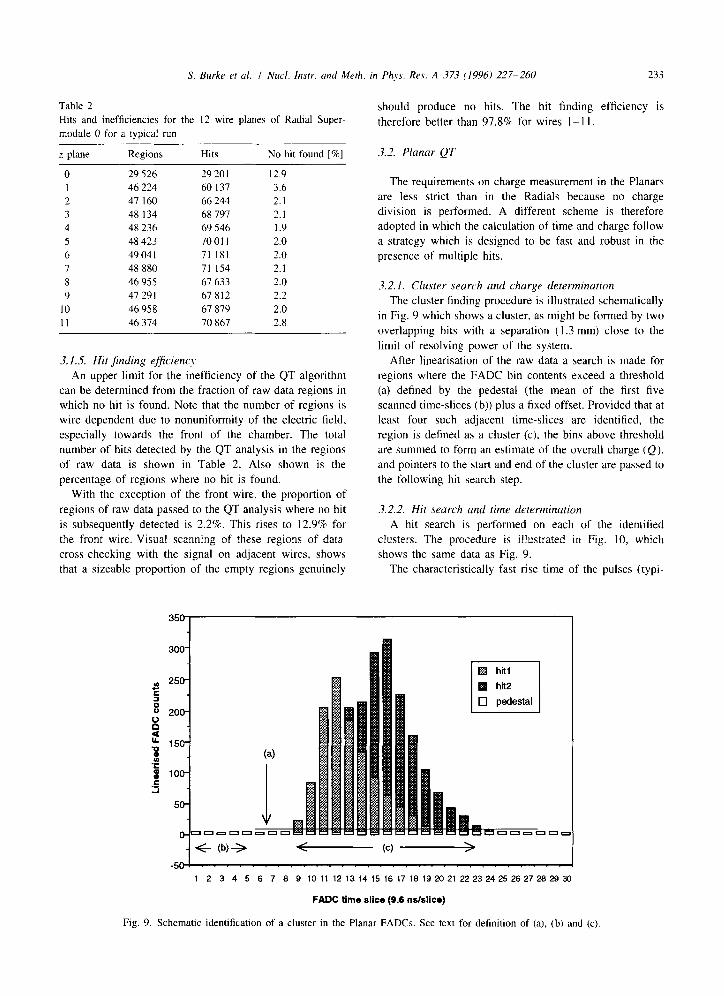
Table 2
Hits and inefficiencies for the 12 wire planes of Radial Super-
module 0 for a typical run
z plane Regions Hits No hit found [%I
0 29 526 29 201 12.9
1 46 224 60 137 3.6
2 41 160 66 244 2.1
3 48 134 68 791 2.1
4 48 236 69 546 1.9
5 48 423 70011 2.0
6 49041 71 181 2.0
7 48 880 71 154 2.1
8 46 9.55 67 633 2.0
9 47 291 67 812 2.2
IO 46 958 67 879 2.0
11 46 374 70 867 2.8
3.1.5. Hit $nding efjcienq
An upper limit for the inefficiency of the QT algorithm can be determined from the fraction of raw data regions in
which no hit is found. Note that the number of regions is wire dependent due to nonuniformity of the electric field,
especially towards the front of the chamber. The total number of hits detected by the QT analysis in the regions
of raw data is shown in Table 2. Also shown is the
percentage of regions where no hit is found.
With the exception of the front wire, the proportion of
regions of raw data passed to the QT analysis where no hit
is subsequently detected is 2.2%. This rises to 12.9% for the front wire. Visual scanning of these regions of data
cross-checking with the signal on adjacent wires, shows that a sizeable proportion of the empty regions genuinely
should produce no hits. The hit finding efficiency is
therefore better than 97.8% for wires 1 -I I.
3.2. Planar QT
The requirements on charge measurement in the Planars are less strict than in the Radials because no charge
division is performed. A different scheme is therefore adopted in which the calculation of time and charge follow
a strategy which is designed to be fast and robust in the
presence of multiple hits.
3.2.1. Cluster seurch and charge determination
The cluster finding procedure is illustrated schematically
in Fig. 9 which shows a cluster, as might be formed by two
overlapping hits with a separation ( 1.3 mm) close to the
limit of resolving power of the system. After linearisation of the raw data a search is made for
regions where the FADC bin contents exceed a threshold (a) defined by the pedestal (the mean of the first five
scanned time-slices (b)) plus a fixed offset. Provided that at least four such adjacent time-slices are identified, the
region is defined as a cluster (cc). the bins above threshold
are summed to form an estimate of the overall charge (Q). and pointers to the start and end of the cluster are passed to
the following hit search step.
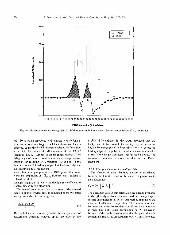
3.2.2. Hit seurch and time determination
A hit search is performed on each of the identified
clusters. The procedure is illustrated in Fig. 10, which shows the same data as Fig. 9.
The characteristically fast rise time of the pulses (typi-
El hi1
q hit2
0 pedestal
-50. .““, ,“. . . . . , “1,. “1
1
FADC slice (9.6 ndslice)
Fig. 9. Schematic identification of a cluster in the Planar FADCs. See text for definition of (a), (b) and (c)
S. Burke et al. I Nucl. Instr. und Merh. in Phys. Res. A 37.7 (1996) .?,77-,760
400
T
-v--v
(4 (W
(4
-100. . . . . . . . . . . . . . y.,..
1 2 3 4 5 6 7 6 9 10 11 12 13 14 15 16 17 16 19 20 21 22 2324 25 2627 28 29 30
FADC time slice (9.6 r&slice)
Fig. 10. Hit identification and timing using the DOS method applied to a cluster. See text for definition of (a), (b) and (c).
tally 30 to 40 ns) associated with charged particle ionisa-
tion can be used as a trigger for hit identification. This is
achieved, as for the Radial chamber analysis. by formation
of a DOS by numerical differentiation of the FADC
spectrum (Eq. (2). applied to single-ended readout). The
rising edges of pulses reveal themselves as sharp positive
peaks in the resulting DOS spectrum ((a) and (b) in the figure). Hits are defined as groups of at least two adjacent bins satisfying two conditions: l each bin in the group must have DOS greater than zero; 9 the hit amplitude, A = Xgroup DOS@), must exceed a
fixed threshold. A single negative DOS bin ((c) in the figure) is sufficient to resolve hits with this algorithm.
The time of each hit, relative to the start of the scanned range in units of FADC bins. is computed as the weighted average over the bins in the group:
t = c n ’ DOS@) A (4)
This technique is particularly stable in the presence of background, which is removed up to first order by the
explicit differentiation in the DOS. Provided that the
background, b, for example the trailing edge of an earlier
hit, can be approximated as linear (b = a + c. n) across the leading edge of the pulse, it contributes a constant level c
to the DOS with no significant shift in the hit timing. The
two-track resolution is similar to that for the Radial
chambers.
3.23. Charge estimation for multiple hits
The charge of each identified cluster is distributed between the hits (k) found in the cluster in proportion to
their amplitudes:
Q,=QA, x.4, -‘. (_ 1- i The quantities used in this calculation are already available to the QT analysis from the cluster and hit finding stages, so that determination of Q, by this method minimises the amount of additional computation. This minimisation can be important when the required rate of raw data reduction is high, but costs some degradation in Qk estimation because of the implicit assumption that the pulse shape is constant (so that Q, is proportional to A,). This is tolerable

S. Burke et al. I Nucl. Insrr. and Merh. in Phys. Res. A 373 (1996) 227-260 235
800
700 _ DOS
- FADC 600
500
400
300
200
100
0
-100
-2oot..“1’.““““.,,““““,““““‘.“““’ 0 10 20 30 40 50 60 70 60
FADC time slice
Rg. 1 I. Hits identified by the Planar hit finding algorithm in
FADC output obtained under normal
Hits 1 and 2 are separated by I .9 mm.
for the Planar chambers. which do by charge division.
3.24. Hit jnding efficiency
HI operating condnions.
not determine position
The thresholds used in the Planar QT algorithm have
been tuned on e-p interaction data to optimise the hit finding efficiency and noise rejection under normal HI
operating conditions. The method, which involves statisti-
cal determination of the number of hits which form aligned
combinations from charged particles traversing single Planar cells, is described in Section 4.5. This hit finding
efficiency is monitored continuously and is normally
greater than 95%. Its high value is confirmed by scanning of Planar FADC spectra from the same data sample, an example of which is shown in Fig. 11, where excellent
agreement is found between the QT identified hits and the leading edges which are evident by eye.
4. Calibration and monitoring of the drift chambers
The drift times from the QT analysis must first be
corrected for timing offsets and then converted into drift distances. When combined with the known location of the sense wires in the HI coordinate frame, these provide preliminary data for use by the pattern recognition and track fitting software. Corrections for track inclination to the wire plane and time-of-flight are made once approxi-
mate track parameters have been determined. Section 4.1 describes aspects of the time-to-distance relation which are common to both the Radial and Planar drift chambers. Special features of the two different types of drift chamber, together with the methods used to calibrate and monitor them, are described in Sections 4.2 to 4.5. Section 4.6 shows how the calibration and monitoring techmques are applied in practice.
4.1. Time-to-distance model
The following model of the drift cells is used to
motivate the choice of time-to-distance function. The
configuration of the drift chambers is depicted schematical- ly in Fig. 12. The electric field lines lie in planes perpendicular to the sense wire as shown in Fig. l2b. For
drift distances, s, greater than about 0.5 cm (measured perpendicularly to the sense wire in the same z plane) the electric field is constant in magnitude and orthogonal to
both the sense wire and the z direction. Closer to the wire, the electric field increases like I/s and turns to point
radially into the wire. To a good approximation, the
isochrones are semicircular. It is assumed that the ionisa-
tion clusters produced nearest to the point where the track
is tangent to the isochrones arrive first and define the
leading edge of the pulse. If the track crosses the drift cell
perpendicularly this point is at the same z as the wire. For
track reconstruction purposes. the drift coordinate of a point on a track is defined as the perpendicular distance from the track to the wire at the z of the wire. The drift distance is first estimated from the measured drift time
assuming that the track crosses orthogonally. For inclined
tracks. a correction to the estimated drift distance must
therefore be applied:
8s = d(sec !J’ - 1) (61
where d, the radius of the isochrones, is approximately
equal to s,, the distance from the wire at which the ionisation begins to drift radially and p is the angle the
track makes with the plane containing the sense wire and the z direction (see Fig. 12b). Close to the wire, d is
replaced by the distance of closest approach of the track to the wire. The correction is made in the final track fit once the track inclination angle is known.
For ionisation drifting towards the sense wire in the same z plane as the wire the absolute value of the drift
velocity remains approximately constant along the drift path. The magnetic field is everywhere orthogonal to the
sense wires and to the electric field. The ionisation drifts
towards the sense wire at a fixed Lorentz angle, (Y, and
Fig. 12. The drift path for ionisation produced at the centre of a cell (a) and from an inclined track (b).

then, close to the wire, the angle decreases as the electric field increases, as shown in Fig. 12a. The component of the
drift velocity perpendicular to the wire therefore increases as the wire is approached. To an adequate approximation, since E is inversely proportional to the drift distance, s, for s<s, and B is constant [II],
tana-IBIIIEI=ps. (7)
Then, the perpendicular component of the drift velocity is
given by
i
Y,
V(s) = y, cos a(s) = qm sss, (8)
IV, = constant s > s,
where V,, the perpendicular component of the velocity at the wire, is equal to the magnitude of the drift velocity (assumed constant throughout the drift space in this
model). The constant /3 can be evaluated in terms of V,, and V,:
\lIl’ - 112 p= “j, .I_ (9)
I I
The time required to drift from a distance s to the wire is
given by:
I-” ds
@) = J,, v(s)
1 & {psdl + /3’s’ + In(ps +ql + p’s’)} sss,
II s - s
t(s,)+i VI
s>s,
(IO)
This equation cannot be inverted in closed form. but an approximation in which the perpendicular component of
drift velocity (hereafter called drift velocity) increases
linearly from V, to V, as s decreases from s, to zero yields drift distances which differ from it by at most IO pm. Fig. I3 shows the drift velocity as a function of s together with the linear approximation. Deviations from this model and the methods used to determine the parameters are dis- cussed in Sections 4.2 and 4.3. Note that, with mean drift
distances of order 2 cm, the mean drift velocity, (V). must be calibrated to better than 0.5% in order to keep sys- tematic errors on the reconstructed distances to less than 100 pm.
4.2. Calibration of the Planar chambers
The geometry and staggered wires of the Planar drift cells (see Section 2.2) allow for a straightforward approach to monitoring and calibration which utilises the known dimensions and symmetries of the cells to maximum effect. In particular it is possible to form statistical check-
Increasing drift field Constant drift field tan a constant
0.9
i
v,/(v)4
1 s (cm)
Fig. 13. Drift velocity as a function of drift distance. The curve corresponds to the model given by Eq. (8).
sums which give a direct measure of chamber performance
and data quality without the need for track reconstruction. These techniques permit effective monitoring and cali-
bration of the chambers as the data accumulate.
J.Z.1. Time-to-distance function for the Planar chantbers The Planar QT algorithm (see Section 3.2) processes the
FADC information from four adjacent wires (one Planar
cell) in a single call, returning the time (t) and integrated pulse size (Q) for every hit found. These times are then transformed to drift distances, s(t) (Section 4.1).
The electric field in the Planar cells is accurately uniform. at -I kV/cm, over 80% of the 28. I mm drift
range, but rises rapidly in the last 5 mm of drift, closest to the sense wire. This causes nonlinearity in s(t), through the
mechanism described in Section 4. I and Fig. 13. The effect
of this nonlinearity is clearly visible between t,, and t, in the Planar drift time distribution shown in Fig. 14. The
25
20 850 ns .~
15
0 200 400 600 800 1000 1200 Dnfi Time (ns)
Fig. 14. Typical Planar drift time distribution with the four knots f, indicated. The approximate velocities on the right hand scale are discussed in the text.

S. Burke et al. I Nucl. Instr. and Meth. in Phys. Res. A 373 (1996) 227-260 231
origin of the knot at tz is not understood. The small rise
before t, is due to double counting of hits from tracks
crossing the cathode plane.
In practice the time-to-distance relation is parametrised in terms of a local velocity which varies linearly with drift
distance, s, over regions si < s < sk + , , where k labels the
knots, in a way which corresponds to the structure which is visible in the drift time distribution (Fig. 14):
v(s)=K+-, ‘kc I
(Sk+, -s,) rk+1 = (V,+, -v,, .
Defining
At:’ ’ = drift time from sL+, to sk
=
(11)
(12)
the integrated drift time, t’, from a point s, <s < sI+, to
the sense wire is
1 (s - Sk) 1 r’(s)=@-t,,)+rL+;In I+----- T,+,TJ (13)
k
with (tr -t,,) = c At:_, II = I
which can be inverted to obtain a parametrised analytic
form for the time-to-distance relation, valid for times in the
region t,<t<tk+,:
s(t)=s, +vkTk+, .{exp[F] - I}, (14)
where t = t’ + t,, is the measured drift time. Two sets of four velocities (V~“‘““, k = 0, I, 2, 3 for the
inner (outer) pair of wires in a cell) and two asymmetry
parameters are sufficient, with the above linear local
velocity model, to provide a good description of the drift properties of a Planar cell. Typical values are shown in
Table 3. The asymmetries, which are caused by electro-
static differences associated with the staggered wires, are used to scale the local velocities by (I fa,) depending on
whether the wire is staggered away from (-) or towards (+) the hit [12]. The a, are determined using the C2 check-sum described in the next Section.
These local drift velocities have been determined, in the
Table 3
Calibrated Planar time-to-distance parameters
li a, .sy [pm] Vy [pm/m] s;‘“’ [km] VT’ [pm/w]
0 0.028 0 44.85 0 46.47
I 0.004 5025 32.87 5025 31.74
2 0.0 16360 33.06 17080 32.93
3 0.0 28 100 28.87 28 100 29.12
first instance, by a direct fit to the drift time distribution on
the inner and outer wires, with the assumption that the
source distribution of hits is uniform in drift distance, s;
g = p = constant (15)
so that
dN dh’ ds dt = -. - = pV(s) .
ds dt (16)
The approximate local velocities which follow from this
assumption, in km/m, can be read from the right hand
scale of Fig. 14. The fit uses Eq. (16). with Eqs. (11) and (13) in a ,$ minimisation having t,,, VT”‘“’ and s:‘““~ as
free parameters but with so”‘“’ fixed at zero and sy”‘“’
fixed at the cell width (28.1 mm). When sp and sy”’ were
fitted independently they were found to be the same;
subsequently they have been constrained to be equal. In
addition there are four free parameters which are required to account for resolution effects at the front and back edges
of the inner and outer drift time distributions. This gives a
total of 16 free parameters to fit about 100 data points (two plots like Fig. I4 where the smooth curve shows the result
of such a fit). The values obtained from such fits (includ- ing the knot at sl) have been confirmed by using the
resulting s(r) parametrisation in the track reconstruction to check that variations in the V, show the track segment fit
residuals to be at a minimum and the number of found
Planar track segments to be at a maximum.
4.2.2. Calibrution and monitoring
Fits of the above type are not performed for every run.
Instead, having determined the V,(N) and mean velocity
V(N) for run number N, the local velocities for later runs are determined by scaling;
V,(N + m) = V,(N) X V(N + m)
v(N) . (17)
The mean velocities, V, are determined to better than
20.3% every two hours on average during normal e-p
running from the width of the drift time distribution and the known cell size (cell width/drift time width
a28.l mm/850 ns = 33 p,m/ns). Typical results from run-by-run calibration are shown in
Fig. 15. The 88 calibrated runs shown there span four days, have a mean drift velocity of 32.854km/ns and an rms scatter of 0.06 p,m/ns. The smallness of this 0.2% rms fluctuation confirms the intrinsic statistical accuracy of the calibration method and the excellent stability of the Planar chamber operating conditions and gas mixture control system [2].
A complementary method for monitoring the stability of drift velocity, which also provides information on intrinsic resolution and data quality, has been developed by making use of the 2300 km stagger of the Planar sense wires.

238 S. Burke et al. I Nucl. Insrr. and Meth. in Phys. Rex. A _173 (1996) 227-260
g 34.0
5 33.5
B g 33.0
e ;; 32.5
B 32.0 - - -
ij
Mean (32.85 m) f 0.5%
z 0 31.5
31 .o 56900 57000 57100 57200 57300
Run Number
Fig. 15. Calibrated mean drift velocities for the Planar chambers.
With some obvious but approximate assumptions con-
cerning linearity and symmetry a charged track of momen-
tum 220MeV/c will produce the following drift times:
T, = + Id, I
TZ = +j Id, + 6 sin(p) + 2yAl
TX = + Id, + 28 sin(
T, = $ Id, + 3S sin(p) + 2yiil
(18)
Here d, is the perpendicular (drift) distance from the track
to wire 1, 6 is the wire spacing (6 mm), !J’ is the angle of the track relative to the plane defined by the wires (Fig.
12), A is the stagger of the wires (?300 p,rn in the s direction), y = ? 1 depending upon the relative sign of A and s for that wire and V is the component of drift velocity
in the s direction. Provided that s has the same sign for all
four wires, i.e. that the track does not cross between the wires, the following check-sums are valid:
c, = (T2 - T, ) - (T, - TX) = 0
2fl.y (19)
cZ=~(T,-T,)-$(T,-T,)=V.
For tracks emerging from the e-p interaction point (on the z axis), the probability of crossing between the wires is very small (of order 300 pm/3 cm = 1%). so the dis-
tribution of C, shown in Fig. 16a shows a sharp peak close to zero. Fig. 16b shows the distribution of C2 for IC,I < 24 ns, with the peaks corresponding to y = +I clearly visible, demonstrating an ability of the Planar chambers to resolve the left-right drift ambiguity. The plots of C, and C, are for cells with one and only one hit/wire.
An estimate of the drift velocity can be obtained from the fitted separation of the peaks in the CZ distribution. The
ratio of the calibrated velocity, determined from the width
of the drift time distribution, to that extracted by this
method, is shown in Fig. 17. It is clear that the velocity determined from the peak
Cl (Is)
x
800
1 .E
700
z 600
500
400
300
200
100
0 -75 -50 -25 0 25 50
c2 (ns)
Fig. 16. (a) Check-sum C, (b) Check-sum C2. The fitted curves
are generalised Breit-Wigner distributions with a smooth back-
ground [19].
separation in the plot of check-sum Cz is significantly lower than the true velocity. This is known to be due to a
small, stagger related, electrostatic asymmetry in the drift
cell [ 121. which is taken into account when formulating the
time-to-distance relation through the asymmetry parame-
56900 57000 57100 57200 57300
Run Number
Fig. 17. The ratio of the drift velocity from the width of the drift
time distribution to that determined from the Cz check-sum versus
run number.

S. Burke et al. I Nucl. Instr. and Meth. in Phys. Res. A 373 (1994) 227-260 239
Fig. 18. Mean resolution of Planar chambers from the Cz check- sum.
ters, a,, of Table 3. The constancy of the ratio verifies that
the above asymmetry does not change with time and gives independent confirmation of the drift velocity stability.
4.2.3. Planur drift measurement precision
From the fitted widths of the peaks in Fig. 16 an
estimate of the single hit resolution can be made; typical results are shown in Fig. 18. The functional dependence of resolution on drift distance can be established by analysing the C, distribution from hits in different bands of drift distance. These results are shown in Fig. I9 with the best
fitting parametrisation (s in cm, fr in pm)
(T* = 165” + s92.3’ + 807’ e-I0 5r (20)
superimposed. The second term models the effect of
diffusion with the third term parametrising the effect of nonuniform drift properties close to the sense wires.
4.3. Calibration of the Radial drift chambers
The wedge-shaped geometry of the Radial drift cell means that the drift time distribution cannot be directly
Dlin Distance (cm)
Fig. 19. Single hit resolution as a function of drift distance in the
Planar chambers. The smooth curve is given by Eq. (20).
00 400 1200 1600 Drift lime (ns)
Fig. 20. Typical drift time distribution in the Radial chambers.
used to obtain a measure of the average drift velocity as is
the case in the Planar chambers. A typical drift time
distribution is shown in Fig. 20. The leading edge of the
distribution is well-defined and can be used to determine t,,. The overall shape however is complex and cannot be
simply mapped into drift velocities. It arises from the wedge shape of ‘the drift cells and nonuniform radial distribution of the hits. In addition, every sense wire
penetrates the region of high hit density at small radius so that the probability of hit loss from two-track overlap is high and depends on the drift distance. (Hits at small drift
distances are more likely to be lost, whatever their radii, than hits at large radii and large drift distance.) The density
and distribution of hits in radius varies with beam and trigger conditions so that a fixed shape is not expected for
the drift time distribution, even if the drift velocities
remain constant.
4.3. I. Time-to-distance function for the Radial chambers
The time to distance function in the Radial chambers is determined by using tracks reconstructed using the Planar
chambers after calibration to predict the true drift distances of hits in the Radials. These distances can then be
compared directly with the measured drift times (after correction for an overall timing offset and propagation time along the sense wires and signal cables). Fig. 21
shows the drift time, scaled by a nominal drift velocity, as a function of predicted drift distance obtained by this
method.
The perpendicular component of the drift velocity is, to a good approximation, independent of both drift distance and radius in the region 20.5 cm from the sense wires; it increases close to the wire as expected from the model discussed in Section 4. I which assumes that the magnitude of the drift velocity remains constant. This approximation may fail within 2 mm from the wire where the electrostatic field is large and the magnitude of the velocity may change significantly. The same parametrisation as that used for the planar chambers (Eq. (14)) is adopted, but only three knots

240
Table 4
Typical calibrated time-to-distance parameters for the Radial drift chambers showing (a) overall parameters and (b) wire-plane dependent
velocity correction factors
k ai .yi bml V, [p,m/ns]
(a) 0 0.0345 0 61.63
1 0.0 4950 37.51
2 0.0 m 37.5 1
Cb)
Wire 0 1 2 3 4 5 6 7 8 9 IO II Factor 0.989 0.999 1.002 1.004 1.004 1.004 1.004 1.004 I .004 1.004 I.004 0.985
and three velocity parameters are needed (Table 4(a)). Note that the last knot at s2 is purely formal: the velocity is
assumed to be constant for drift distances greater than s,.
The appropriate limiting forms of Eqs. (1 l)-( 14) for
r,_ -+m are used to compute the drift distance in this
region. Data like those in Fig. 21 are obtained for each run
containing a reasonable number of events (-10 000) and
are used to determine the velocity V, . Independent straight line fits are made for positive and negative drifts in the range 0.6 5 IsI 5 3.5 cm. The velocity is calculated from the weighted mean of the two slopes. A precision of about
0.2% is obtained. The velocity V, and location of the knot
point S, can also be deduced from the same data. To a
good approximation, these are found to scale with V, and a separate run-by-run determination is not necessary.
The electrostatic field configuration is not identical for
all the wires in the Radial chambers. Consequently the average drift velocities near the front of the drift chamber
are significantly lower than in the middle. These inhomo- geneities are treated by applying scaling factors to the velocities on each of the twelve wire planes (Table 4(b)).
As is the case for the Planar chambers, an asymmetry arising from the wire stagger is seen and is corrected for
-4 -2 0 2 4 Drift Distance (cm)
Fig. 21. Scaled drift time versus predicted drift distance. The insert shows the region at short drift distances.
by applying a different scale factor to the velocities for hits
on wires staggered towards or away from the track. This
correction can only be applied once the sign of the drift
coordinate has been resolved by the reconstruction soft- ware. These characteristics, including the wire-dependence
of the drift velocities, have been qualitatively confirmed by an electrostatic simulation of the drift chambers using the
GARFIELD [ I3 ] program.
4.3.2. Monitoring of the drift velocities in the Radial chambers
The above technique can be used as a monitor of the drift velocities only after track reconstruction has taken
place. A fast monitor of changes in parameters is desirable in order to avoid mis-reconstruction of the tracks and the
need to reprocess the data. To this end, some of the
techniques already described for the Planar chambers are
exploited. Although no drift velocity information can be extracted
from the drift time distribution alone, by making use of the charge division measurement it is possible to make drift time distributions in slices of radius, for which the drift
cells have approximately constant width and so are more akin to those in the Planars. This allows the determination of the maximum drift time as a function of radius. Since
the cell is wedge-shaped this time should increase linearly with radius given that the drift velocity is constant in the
relevant region away from the sense wire. The slope is thus
a direct measure of the drift velocity in the constant drift field region. A fit is performed over a restricted range, 30 cm <R < 60 cm, in order to avoid end-effect distor-
tions. Fig. 22 shows the location of the maximum drift time as a function of the radius, for two different gas mixtures, with the linear fits superimposed. The method is vulnerable to the imprecision of the radius measurement which smears the back edge of the drift time distributions. In addition, the imprecision itself depends on the hit density and so beam and trigger conditions can affect the result. Also, as a result of the Lorentz angle, the linear relationship depends on which side of the wire plane the hit originated and this cannot be determined at the single hit level. Consequently this method gives a drift velocity with an uncertainty of about 1%.

S. Burke et al. I Nucl. Instr. and Meth. in Phys. Res. A 373 (19961 227-260 241
measured using test-pulses, and resistances and resistivities
were measured as part of a full chamber survey before
installation. The measured relationship between the charge
division variable (Q’ - Q-)/(Q + + Q -) and radius is linear.
4.3.4. Precision of the drift and radius measwements
250
0 0 10 20 30 40 50 60 70 80
Radius (cm)
Estimates of the single hit drift resolution and its dependence on drift distance are obtained from an analysis
of C, check-sum distributions as described for the Planar
chambers in the previous Section. Using the same func-
tional form to parametrise the resolution gives (Fig. 24)
IT’ = I .9’ + ~127.1’ + 317’e-’ ‘Is , (21) Fig. 22. Maximum drift time versus radius for two gas mixtures.
giving a mean resolution = 180 p.m.
A Radial cell has 12 wires in depth; these can be taken
in groups of four and the same check-sums as for the
Planars can be calculated and monitored. The Cl check- sum gives another measure of the drift velocity. The
relationship between this velocity and the average drift velocity in the cell differs from that in the Planars because
of the differing disposition of field wires. The run to run
variation in this drift velocity is about 0.5% during stable
periods of running and the method is less susceptible than
the drift time versus radius method to beam conditions. Fig. 23 shows the drift velocity measurements obtained
for a series of data runs by the above methods. The ratios of the different velocity parameters remain constant from
run to run so that the fast monitoring methods can be used to effect a rapid recalibration in the event of a significant
change in operating conditions (see Section 4.6).
The method of track projection from the Planar cham- bers is used to check the radial coordinate determination.
The best resolution of about 1.5 cm is achieved only for the larger pulses. The average resolution for isolated hits is
3-4 cm. More seriously, because of the high hit density, a
substantial fraction of hits overlap. The radius measure- ment may be significantly degraded for such hits.
1.1. Determination of t,,
4.3.3. Culibration of the charge division measurement
Planar-based tracks are also used to calibrate the de-
termination of the radial coordinates of the hits by charge division. The charge division measurement is not sensitive
to the absolute charges, so frequent run-dependent cali-
brations are not needed for this purpose. The relative gains
of the preamplifiers at the two ends of the wire-pair are
Before application of the time-to-distance functions, various corrections are applied to the times determined by the QT analysis. An average offset from the trigger time, t,. is determined for each data run by locating the leading
edge of the drift time distribution of the hits. This is done by numerical differentiation of the drift time distribution to
obtain a positive peak corresponding to the rising front edge. The fitted time of this peak is used to define the
timing offset to an accuracy of -0.5 ns for a typical run.
Fig. 25 shows the t, values, as determined by this
method, over a two month period in 1993. Discontinuous
changes. due to known hardware modifications, are clearly
30 - -he 19)
25 56500 57ow 57100 57200 57300
Run Number
Fig. 23. Drift velocity measurements for a series of runs from the Fig. 24. Single hit resolution as a function of drift distance in the three methods. Radial chambers.
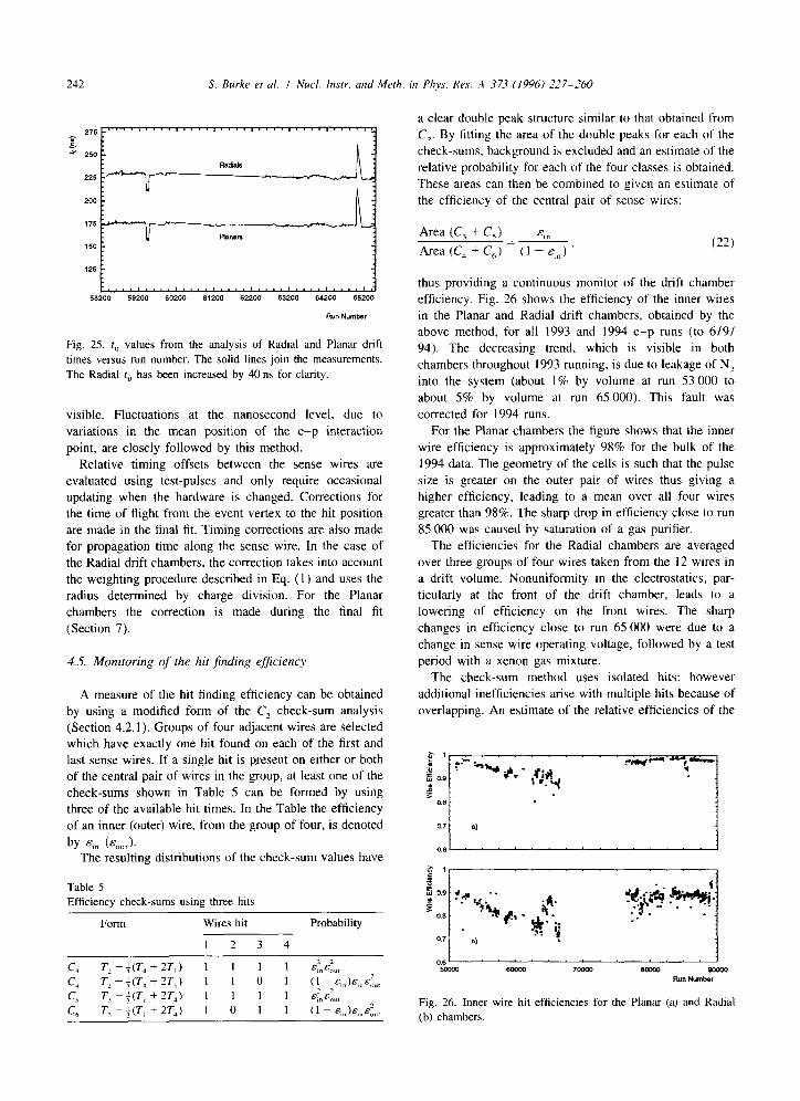
242 S. Burke et al. I Nucl. Instr. and Meth. in Piys. Res. A .17-T (1996) 777-30
R”” Number
Fig. 25. I, values from the analysis of Radial and Planar drift
times versus run number. The solid lines join the measurements.
The Radial t, has been increased by 40 ns for clarity.
visible. Fluctuations at the nanosecond level, due to
variations in the mean position of the e-p interaction
point, are closely followed by this method.
Relative timing offsets between the sense wires are evaluated using test-pulses and only require occasional
updating when the hardware is changed. Corrections for the time of flight from the event vertex to the hit position are made in the fmal fit. Timing corrections are also made
for propagation time along the sense wire. In the case of the Radial drift chambers, the correction takes into account
the weighting procedure described in Eq. ( I ) and uses the
radius determined by charge division. For the Planar chambers the correction is made during the final fit
(Section 7).
3.5. Monitoring of the hit finding efficiency
A measure of the hit finding efficiency can be obtained
by using a modified form of the C, check-sum analysis (Section 4.2.1). Groups of four adjacent wires are selected which have exactly one hit found on each of the first and last sense wires. If a single hit is present on either or both of the central pair of wires in the group, at least one of the
check-sums shown in Table 5 can be formed by using three of the available hit times. In the Table the efficiency
of an inner (outer) wire, from the group of four, is denoted
by ~8, (E,,,). The resulting distributions of the check-sum values have
Table 5
Efficiency check-sums usiw three hits
Form Wires hit Probability
a clear double peak structure similar to that obtained from
C,. By fitting the area of the double peaks for each of the check-sums, background is excluded and an estimate of the
relative probability for each of the four classes is obtained.
These areas can then be combined to given an estimate of the efficiency of the central pair of sense wires:
Area (C, + C,) 4, =-
Area(C,+C,) (l-c,,)’ (22)
thus providing a continuous monitor of the drift chamber efficiency. Fig. 26 shows the efficiency of the inner wires in the Planar and Radial drift chambers, obtained by the above method. for all 1993 and 1994 e-p runs (to 6/9/
94). The decreasing trend, which is visible in both
chambers throughout 1993 running, is due to leakage of Nz into the system (about 1% by volume at run 53 000 to
about 5% by volume at run 65 000). This fault was
corrected for 1994 runs. For the Planar chambers the figure shows that the inner
wire efficiency is approximately 98% for the bulk of the
1994 data. The geometry of the cells is such that the pulse size is greater on the outer pair of wires thus giving a higher efficiency, leading to a mean over all four wires
greater than 98%. The sharp drop in efficiency close to run 85000 was caused by saturation of a gas purifier.
The efficiencies for the Radial chambers are averaged
over three groups of four wires taken from the I2 wires in a drift volume. Nonuniformity in the electrostatics, par-
ticularly at the front of the drift chamber, leads to a lowering of efficiency on the front wires. The sharp
changes in efficiency close to run 65 000 were due to a
change in sense wire operating voltage, followed by a test
period with a xenon gas mixture.
The check-sum method uses isolated hits: however
additional inefficiencies arise with multiple hits because of overlapping. An estimate of the relative efficiencies of the
0.6’ . 1
Fig. 26. Inner wire hit efficiencies for the Planar (a) and Radial
(b) chambers.
S. Burke et ~1. I Nucl. Instr. and Meth. it1 Phys. Res. A 37.3 (1996) 227-260 243
different wire planes can be obtained by making a simple
ratio of the number of hits found per wire relative to the
wire with the most hits. This method gives an efficiency of
100% for the wire with most hits. For the planars the two methods are in reasonable agreement as the basic unit is a four wire group. For the radials there are 12 wires in a cell and the absolute measurement is performed independently
for the front, middle and back four wires. The relative efficiencies have to be scaled by the absolute efficiency to arrive at efficiencies for all 12 wires. These wire efficien-
cies for 1993 and 1994 data are given in Table 6 and
provide the input to the detector simulation (see Section
9.1).
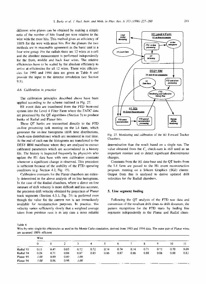
4.6. Culibration in practice
The calibration principles described above have been applied according to the scheme outlined in Fig. 27.
HI event data are transferred from the FTD front-end system into the Level 4 Filter Farm where the FADC data
are processed by the QT algorithms (Section 3) to produce banks of Radial and Planar hits.
These QT banks are transmitted directly to the FTD on-line processing task running on the L4 farm, which
generates the on-line histograms (drift time distributions,
check-sum distributions) which are monitored in real time. At the end of each run the histograms are transferred to the
DESY IBM mainframe where they are analysed to extract
calibrated parameters which are accumulated in a history file. The history is inspected frequently by physicists who
update the Hl data base with new calibration constants whenever a significant change is observed. This procedure is sufficient because of the stability of the FTD operating conditions (e.g. Section 4.2, Fig. 15).
Fig. 27. Monitoring and calibration of the Hl Forward Tracker
Chambers.
determination than the result based on a single run. The
value obtained from the C, check-sum is still used as an important monitor and to detect significant discontinuous
changes.
Calibration constants for the Planar chambers are entire- ly determined in the above analysis of on-line histograms.
In the case of the Radial chambers, where a direct on-line
measure of drift velocity is more difficult and less accurate,
the precision drift velocity obtained by projection of Planar
track segments (Section 4.3.1; Fig. 21) is preferred even though the value for the current run is not immediately
available for reconstruction purposes. In practice, this
velocity varies sufficiently slowly that a weighted average taken from previous runs is in any case a more reliable
Constants from the Hl data-base and the QT banks from the L4 farm are passed to the Hl event reconstruction program, running on a Silicon Graphics (SGI) cluster. Output from this is analysed to derive updated drift
velocities for the Radial chambers.
5. Line segment finding
Following the QT analysis of the FTD raw data and
conversion of the resultant drift times to drift distances, the
pattern recognition for the FTD starts by finding line segments independently in the Planar and Radial cham-
Table 6 Wire-by-wire single-hit efficiencies as used in the Monte Carlo simulation, derived from 1993 and 1994 data. The outer pair of Planar wires
are assumed 100% efficient
Wire
0 I 2 3 4 5 6 7 8 9 10 II
Radial 93 0.11 0.47 0.65 0.72 0.72 0.74 0.74 0.74 0.7 1 0.73 0.70 0.69 Radial 94 0.24 0.7 I 0.84 0.87 0.85 0.86 0.87 0.86 0.88 0.88 0.88 0.83 Planar 93 1.00 0.89 0.89 1.00 Planar 94 1.00 0.98 0.98 1.00
244 S. Bde et al. I Nucl. Instr. rwd Meth. it1 Ph?s. Rrs. A 37.1 f 1996) 27-260
bers. Due to the different geometries of the chambers the procedures used are independent and are described separ- ately in the two following Sections.
5.1. Line segment finding in the Planar chambers
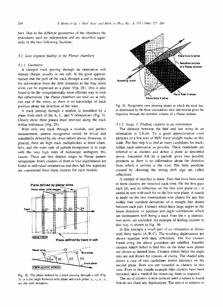
5.1. I. Geometry A charged track passing through an orientation will
deposit charge, usually in one cell. In the good approxi- mation that the path of the track through a cell is straight,
the information from the drift distances to the four sense
wires can be expressed as a plane (Fig. 28). This is also found to be the computationally most efficient way to treat this information. The Planar chambers are read out at only one end of the wires, so there is no knowledge of track position along the direction of the wire.
A track passing through a module is described by a
plane from each of the X, U, and V orientations (Fig. 4).
Clearly these three planes must intersect along the track within tolerances (Fig. 29).
With only one track through a module, and perfect
measurement, pattern recognition would be trivial and completely defined by the observations above. However, in
general, there are high track multiplicities in these cham-
bers, and the main task of pattern recognition is to cope with the very high rates of hodoscope ambiguity this causes. There are two distinct stages to Planar pattern recognition: firstly clusters of three or four digitisations are found in individual orientations and then full line segments
are constructed from these clusters for each module.
Plane defined by Planar wires
Plane defined by track in cell
Fig. 28. The plane defined by a track passing through a cell (Fig. 5). (Y is the angle between wire plane and track plane. s,. s?, s,, s4
are the drift distances.
s from U wires
nsitlvs volume s Planar module
lncoml
_ Planeirom V wires Plane from X wires
Fig. 29. Perspective view showing planes in which the track lies,
as determined by the three orientations; their intersection gives the
trajectory through the sensitive volume of a Planar module.
5.1.2. Stage 1: Finding clusters in an orientation The distance between the first and last wires in an
orientation is 1.8 cm. To a good approximation even
particles of a few tens of MeV leave straight tracks on this
scale. The first step is to find as many candidates for tracks within each orientation as possible. These candidates are
referred to as clusters and define a plane as described above. Ionisation left by a particle gives two possible positions as there is no information about the direction from which it arrived at the wire. The false positions
created by choosing the wrong drift sign are called
reflections. A number of searches is made. Data that have been used
to form clusters are removed each time. On the first pass
each hit. and its reflection, on the first wire plane in : is
paired in turn with each hit on the last wire plane. A search is made on the two intermediate wire planes for any hits
within four standard deviations of a straight line drawn between each pair. Clusters which have large angles to the beam direction, or position and angle correlations which are inconsistent with being a track from the e-p intersec- tion point, are excluded. An example of finding clusters in
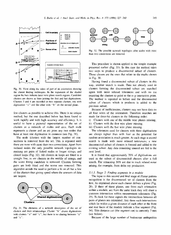
this way is shown in Fig. 30. In this example a small part of an orientation is shown
with three tracks (A, B, C). The resulting digitisations are shown together with their reflections. The five clusters found using the above procedure are labelled. Possible clusters which failed to find hits on the inner wire planes are shown as dashed lines. Clusters which failed the angle cuts are not shown for reasons of clarity. The shaded area shows a case of two candidates within tolerance on the second plane. Both sets are recorded as clusters in this case. Even in this simple example false clusters have been recorded, and a method for removing them is required.
The set of clusters is now reduced until a subset is found that do not share any digitisations. The aim is to remove as
S. Burke et al. I Nucl. Instr. arid Meth. in Phys. Res. A 373 (1996) 227-260 245
- Pdtlons Of
dlgltlsatlons
A track A + track B x track C
manions shov.n in lighu pr,nt
1 _ selected cluster
Fig. 30. View along the wires of part of an orientation showing
the cluster finding techniques, In the expansion of the shaded
region the bars indicate inner wire plane search regions, Candidate
clusters are shown as lines joining the first and last digitisations.
Clusters 3 and 4 are recorded as two separate clusters, one with
digitisation “a” and the other with “b” on the second plane.
few clusters as possible to achieve this. There is no unique
method, but the one described below has been found to
work rapidly and with high accuracy and efficiency. It is useful to have a pictorial representation of the set of
clusters as a network of nodes and arcs. Each node
represents a cluster and an arc joins any two nodes that
have at least one digitisation in common (see Fig. 31). The node (cluster) with the largest number of con-
nections is removed from the set. This is repeated until there are none with more than two connections. Apart from isolated nodes the only possible network topologies re- maining are pairs of linked nodes or longer strings, and closed loops (Fig. 32). All clusters in loops are fitted to a
straight line, as are clusters in the middle of strings, and the worst fitting candidate is removed. Clusters forming
pairs are both fitted and the worse one removed. This
algorithm avoids the need to perform a fit on all but a few
of the clusters thus giving speed where the amounts of data are largest.
Fig. 31. The elements of a network description of the set of clusters and their relationships. Cluster “b” shares digitisations with clusters “a” and “c”, but there is no sharing between “a” and “c”.
h&tad ,:,::::j:j : :.
. . . . . . . . . . . ~ ~ ‘OoP Q : ::..
string
Fig. 32. The possible network topologies after nodes with more
than two connections are removed.
This procedure is shown applied to the simple example
presented earlier (Fig. 33). In this case the method takes two steps to produce a disconnected subset of clusters.
Those chosen are the ones that relate to the tracks shown
in Fig. 30.
Having found a disconnected subset of clusters in this way, another search is made. Data not already used in
clusters forming the disconnected subset are searched
again with more relaxed tolerances and with no cut requiring the clusters to point to the e-p interaction point.
The method is repeated as before and the disconnected subset of clusters which it produces is added to the previous subset.
Because of inefficiencies, clusters may not have data on
all four wires of the orientation. Therefore searches are made for three-hit clusters in the following order:
i) Clusters with one of the middle wire planes missing, ii) Clusters with the first wire plane missing,
iii) Clusters with the last wire plane missing.
The tolerances used for clusters with three digitisations are always tighter than with four as the potential for
random association is much greater. At each stage a second search is made with more relaxed tolerances; a new
disconnected subset of clusters is formed and added to the existing subset. Any data remaining unused are fed to the next level.
It is found that approximately 70% of digitisations are
used in the subset of disconnected clusters after a full
search. The remaining 30% are due to track related noise arising, for example, from delta ray production.
51.3. Stage 2: Finding segments in a module
The input to this second and final stage of Planar pattern recognition is the disconnected set of clusters from the
first. As explained above each cluster defines a plane (Fig, 28). If three of these planes, one from each orientation within a module, are from the same track they will share a common intersection within measurement tolerances (Fig. 29). To look for these signals the intersections between all pairs of planes are calculated. Any three such intersections which lie within a given distance of each other at the front and rear faces of the module indicate a line segment (Fig. 34). This distance cut (the segment cut) is currently 7 mm (see below).
Because of the large number of hodoscope ambiguities

246 A .17.3 (1996) 127-260
1 . 1 1 \ I
SW (4 SW W
Fig. 33. An example of finding the disconnected subset of clusters for the case shown in Fig. 30. In step (a) the most highly connecrtd node
is removed, in step (b) the connected pair 3/4 is fitted and the worse removed.
even small numbers of tracks produce a large number of
false line segments (Fig. 37 [I]). Most of these can be removed by selecting the subset of line segments that does
not share digitisations. The method chosen to achieve this can again be
illustrated using a network of nodes and arcs. As before the
method is not unique but has been found. from Monte
Carlo studies, to select an almost complete set of correct line segments with few false segments for typical multip-
licities (less than 20).
The digitisations belonging to each line segment are
fitted to a straight line and the probability calculated. Each
node (line segment) is given a weight which is the sum of the probabilities of all nodes connected to it (not including itself). The node with the highest number of connections is then removed. If this node is not unique then, of the nodes
with the highest number of connections, the one with the highest weight is removed. This procedure is repeated until a disconnected set of nodes remains (i.e. no line segments
share digitisations).
A simple example of this procedure is shown in Fig. 35. Initially there are nine connected nodes with fit prob-
abilities and weights as shown in Fig. 35 (i). Nodes 4 and
6 both have five connections, but 6 has the highest weight (3.26) and is therefore removed (Fig. 35 (ii)). The node
Distances testa
Fig. 34. Three intersections between pairs of planes. If all the distances represented by dashed lines are less than 7 mm then the
three clusters/planes producing these intersections are selected as
a line segment.
weights and connections must now be recalculated. Node 4 still has the highest number of connections and is now removed (Fig. 35 (iii)), followed by node 8 (Fig. 35 (iv)). Finally node 1 is removed, as it has the higher weight, and a disconnected set of segments is found.
This method used for segments is more elegant than that
used for clusters and is possible because the smaller number of segments enables the algorithm to be more
computationally intensive.
5.2. Performance of the Planar pattern recognition
The effectiveness of the method described was measured using a Monte Carlo simulation. Muon tracks were gener- ated with 100% digitising efficiency which evenly popu-
lated the mD in angle and with a flat momentum distribution between 0.5 and 50 GeVlc. A two-track res- olution of 2 mm was assumed. The efficiency for finding good clusters is shown as a function of the number of
tracks through the RD (Fig. 36). The efficiency is above 95% even for 40 tracks (Fig. 36a); the number of losses
and mistakes is small (Fig. 36b). The method for finding
clusters will construct essentially all those which survive the intrinsic resolution for two tracks; however, many false
ones are also created. This plot shows that it is possible to regain the correct sample by selecting a disconnected
subset as described above. The percentages of good segments in the total popula-
tion of all found segments (a) and separately in the disconnected set (b) are shown in Fig. 37 [I] using a segment cut of 3 mm (see Fig. 34). A good segment is defined here as one which has at least 9 out of a potential 12 hits from the same Monte Carlo (genuine) track. This sample, however, predominantly consists of segments formed with 12 hits from the same track. The fraction of all segments formed which are good falls to 50% for 15 tracks and 20% for 40, but the proportion of good segments in the chosen disconnected subset stays at almost 100% for 20 tracks. By choosing a disconnected subset of the segments some of the good segments found are then

S. Burkr et al. I Nucl. Instr. and Meth. in Phys. Res. A 373 (1996) Z7-260 241
Fig. 35. The sequence (i) to (iv) shows how a disconnected set of line segments is obtained.
excluded, and this percentage is shown by the histogram
(c). It is noted that this percentage matches very closely the percentage of false segments in the subset ((b) + (c) =
100%). This shows that the disconnected subset contains approximately the true number of segments. Fig. 37 [II]
shows the efficiency to find a genuine segment in the disconnected subset as a function of track multiplicity (a):
also shown is the contamination (b). The subsequent analysis uses only segments in the disconnected subset.
In real data, because of problems beyond the intrinsic digitisation resolution. a segment cut of 7 mm is currently
Number of Tracks in Forward Tracker
Fig. 36. Planar code performance as a function of track multiplici-
ty: (a) 4.hit clusters formed with no mistakes and (b) 4-hit clusters
with one mistake or 3-hit clusters with no mistakes.
required, and the efficiencies for this value are shown in
Fig. 37 [III] and [IV]. If the knowledge and the functioning of the chambers and associated electronics were perfect
and given an intrinsic point resolution of -200 km, a cut
of less than 3 mm could be used. It can be seen that going
to the higher value cut causes a significant degradation. For the majority of the data the probability of losing
more than one hit per cluster is very small (see Table 6). However in a non-negligible number of cases there is a
loss of more than one digitisation or even the correlated loss of a whole cluster (see Section 9.1). An extension to
the segment finding method described above is therefore being developed. Segments are constructed from any
unused data using two clusters confirmed by only one or two digitisations in the remaining orientation. A discon-
nected set of these is formed and added to the existing set.
Finally, from any remaining data, segments are formed
from two clusters alone and another disconnected set is added to the above.
5.3. Line segment jinding in the Rudial chambers
The procedure that has been adopted is to search for straight line segments in drift based on triplets of adjacent points. Line segment finding is carried out wedge by wedge. Within a wedge all triplets of digitisations are selected that satisfy the criterion
It@, +d,)-d,l<P, 1 (23)

60
c) i”i c-...I ,,,. I,,_
5 10 15 20 25 30 35 ‘0 5 10 15 20 25 30 35
Number of Tracks in Forward Tracker Number of Tracks in Forward Tracker
If1 Ill11
60 -
Number of lrocks in Forward Tracker Number of Tracks in Forward Tracker
Fig. 37. Planar code performance as a function of track multiplicity: [I] (a) percentage of all segments which are good, (b) percentage of
segments in the disconnected set which are good and Cc) percentage of good segments lost by choosing the disconnected set. [II] (a)
percentage of genuine track segments found in the disconnected set and (b) percentage of segments which are not good (see text). [III] and
[IV] are the same as [I] and [II] but with a 7 mm rather than a 3 mm segment cut.
where d,, d,, d, are signed distances to the wire plane and P, is a parameter (approximately I mm).
For the majority of triplets, this resolves the left-right ambiguity of the three points and gives the sign of the drift. The next step is to join the triplets. This is done if
triplets have points in common with the same drift sign, and the resultant group of hits lies within a certain tolerance of a straight line joining the first and last points of the group. If triplets are separated by one missing digitisation, they may also be associated if they satisfy this straight line criterion. The associated triplets are then fitted to a straight line. The parameters of this fit are used to project along the wedge and associate isolated digitisations
with the joined triplets. At this point there is a set of
potential line segments of which the best is selected. either as that line segment with the maximum number of points or, if the two longest segments have the same number of points, that with the best x2 to a straight line. The points making up the line segment are marked used, the points are recorded and the program returns to re-examine remaining points in the wedge or transfers to the next wedge if insufficient digitisations remain to form a line segment.
The procedure described above finds points belonging to a track segment provided that it lies entirely within one Radial wedge. In practice, this may not be true. Since

S. Burke et al. I Nucl. hutr. and Meth. in Phys. Res. A 373 (19961 227-260 249
tracks are, to a good approximation, straight lines in 4-z
line segments can be extrapolated in 4 into nearby wedges
to pick up associated digitisations.
6. Line segment linking
6. I. The track model
The line segments forming a track lie on a helix. A helix
fit could be used to check if a set of line segments is
consistent with belonging to a track, but this would be prohibitively expensive in computer time. Consequently an approximate track model is used to represent a helix and this track model is used to link line segments and to verify
that the line segments are consistent with lying on a helix.
With the definitions:
R=((x-x‘,)-+(v~v,)~)“’ (25)
where x, y are the coordinates of a point on a track, and
with 0 as the polar angle of the track with respect to the
z-axis, the helical trajectory of a particle, momentum P. charge Q, passing through the known point xz,, y,,, I,., is
given by
4= 4’: + $,,
R(z) = tan(o) sin( J’(z - z,,))
*I &J
(26)
(27)
where $’ = (KPcos(0)))‘, K = -2/B&, B is the mag- netic field (along z-axis) and c is the velocity of light.
For tracks that have originated close to the z-axis (x, =
y,, = 0), e.g. tracks from the primary vertex, it follows from Eqs. (26) and (27) that a good track model is
4(z) = 4’z + 4,,, (28)
irrespective of momentum, and provided that 4’ is small
(i.e. high momentum) then
R(z) = R’z + R,, (29)
where tan(4) = v/x and R = {.Y’ + y’}“‘. Thus the helix is approximated by straight lines in 4-z and R-z. For off-
axis tracks, the 4-z relation is well approximated by a
parabola; the R-z relation becomes parabolic both for off-axis tracks and for low momenta. These representations allow the Planar and Radial chambers to be treated in an identical manner.
The coordinate W (Fig. 38) is given by W = y cos(a) - x sin(a), where (Y is the azimuthal angle of the Planar or Radial wire. If a track model has been defined in 4-z and ff-;, the coordinate, W(z), at a given z is given by
)X
Fig. 38. The coordinate W measured by sense wires at an angle Q.
W(z) = R(i) sin( &;) - a) + y,. COS((Y) ~ xy sin(a) (30)
Thus a ,$ evaluated in drift can be used to determine whether the track model is consistent with the measured
drifts and hence verify that the line segments are correctly
linked. Note that while Eqs. (28) and (29) are adequate
representations for a track through the Radial chambers
(due to the small values of 4 - (Y), it is essential to use Eq. (27) or a parabolic relation in R-2 if Eq. (30) is used for
the Planar chambers. There are four steps in the linking of segments to form
tracks: firstly, the line segments found in the Planar
chambers are joined to form potential tracks and these tracks are in turn linked to Radial line segments. Secondly,
and independently. Radial segments are linked to form tracks that are in turn linked to Planar line segments. Due
to chamber inefficiencies and two-track resolution neither
procedure finds all tracks, so in a third step the tracks
found in the first two steps are compared and the best selected. In a final step unlinked Planar segments are
joined to unlinked Radial segments where possible. The
following three Sections describe these procedures in
detail.
6.2. Track jinding using the Planar line segments
The Planar line segments are fitted to straight lines in X-,: and y-z. These parameterisations are readily con-
verted to 4 and R so that the approximate helix representa- tions of Section 6.1 can be used to verify the linkage of
Planar segments. The first operation is to join the Planar line segments to
form tracks. This is done pair-wise by projecting the segments to a plane midway between them. For high
momentum tracks the pitch of the track helix is much greater than the separation of the planar modules, so these segment projections to the midplane have approximately the same X, ?; (within 1 mm for tracks of momentum greater than 0.5 GeV/c). Line segments are linked to form a track if D =(.u, -x2)’ + (JJ, -yz)’ CD,,,,,, where-r,, _v, (x2, vr) are the coordinates of the projections of line segments l(2) and D,,,_ is a parameter presently set to
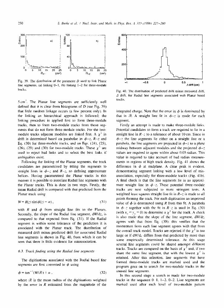
250 S. Burke et (11. I Nucl. Itrstr. urrd Met/l. irl Phys. Kes. A 37.3 (1996) 227-260
0 5 10 15 20 25 0 5 10 15 20 25
DO.1 (cm*) ~1.2 (CW
Fig. 39. The distribution of the parameter D used to link Planar line segments, (a) linking O-1, (b) linking l-2 for three-module tracks.
5 cm’. The Planar line segments are sufficiently well
defined that it is clear from histograms of D (see Fig. 39)
that little random linkage occurs (a few percent only). In
the linking an hierarchical approach is followed; the
linking procedure is applied first to form three-module
tracks, then to form two-module tracks from those seg- ments that do not form three-module tracks. For the two- module tracks adjacent modules are linked first. A x’ in
drift is determined based on parabolae in 4-z. R-z and
Eq. (30) for three-module tracks, and on Eqs. (24), (25), (26), (29) and (30) for two-module tracks. These ,$ are used to reject bad links and to select the best links if
ambiguities exist. Following the linking of the Planar segments, the track
candidates are parametrised by fitting the segments to
straight lines in 4-z and R-z, so defining approximate
helices. Having parametrised the Planar tracks in this
manner it is possible to associate Radial line segments with the Planar tracks. This is done in two steps. Firstly, the mean Radial drift is compared with that predicted from the
Planar track using
W = R(z) sin(&z) - cu) , (31)
with R and 4 from straight line fits to the Planars. Secondly, the slope of the Radial line segment, dW/dz, is
compared to that expected from Eq. (31). If the Radial segment is within some tolerance of the prediction it is
associated with the Planar track. The distribution of measured drift minus predicted drift for associated Radial
line segments is shown in Fig. 40, from which it can be seen that there is little evidence for misassociation.
6.3. Track jnding using the Radial line segments
The digitisations associated with the Radial based line segments are first converted to C#J using
C$ = tan~‘(Wl8) + 0, (32)
where Z is the mean radius of the digitisations weighted by the error in R estimated from the magnitude of the
oc -1 -0.5 0 0.5 1
A dtifl (cfn)
Fig. 40. The distribution of predicted drift minus measured drift.
A drift. for Radial line segments associated with Planar based
tracks.
integrated charge. Note that the error in 4 is dominated by
that in 2. A straight line fit in 4-z is made for each
segment.
Firstly an attempt is made to make three-module links. Potential candidates to form a track are required to lie in a
straight line in R-z to a tolerance of about IO cm. Since in 4-2 the line segments lie either on a straight line or a parabola, the line segments are projected in 4-2 to a plane
midway between adjacent modules and the projected 4-z values are required to agree within about 0.05 radian. This
value is required to take account of bad radius measure-
ments in regions of high track density. Fig. 41 shows the
difference in Q, at midplane. A clear peak is evident,
demonstrating segment linking with a low level of mis-
association, especially for three-module tracks (Fig. 41 b). A final check is that the line segments lie in an approxi-
mate straight line in 4-z. These potential three-module tracks are next subjected to more stringent tests. A weighted least squares straight line fit in R-z is made to all
points forming the track. For each digitisation an improved value of C$ is determined using R from this fit. A parabola
in 4-z together with the fit in R-z is used in Eq. (30) (with x” = y,, = 0) to determine a xz for the track. A check
is also made that the slope of the line segment, dW/d:.
agrees with that from Eq. (30); this verifies that the momentum from each line segment agrees with that from the overall track model. Tracks are rejected if the x’ is too
large or if dW/dz differs from that predicted by more than some empirically determined tolerance. At this stage several line segments could be shared amongst different tracks. Tracks are compared on the basis of x2 and, if two share the same line segment, that with the lowest xz is retained. After this selection, line segments that have formed three-module tracks are marked used and the program goes on to search for two-module tracks in the unused line segments.
In this second stage a search is made for two-module tracks in the sequence O-l, l-2, O-2. Line segments are marked used after each level of two-module pattern
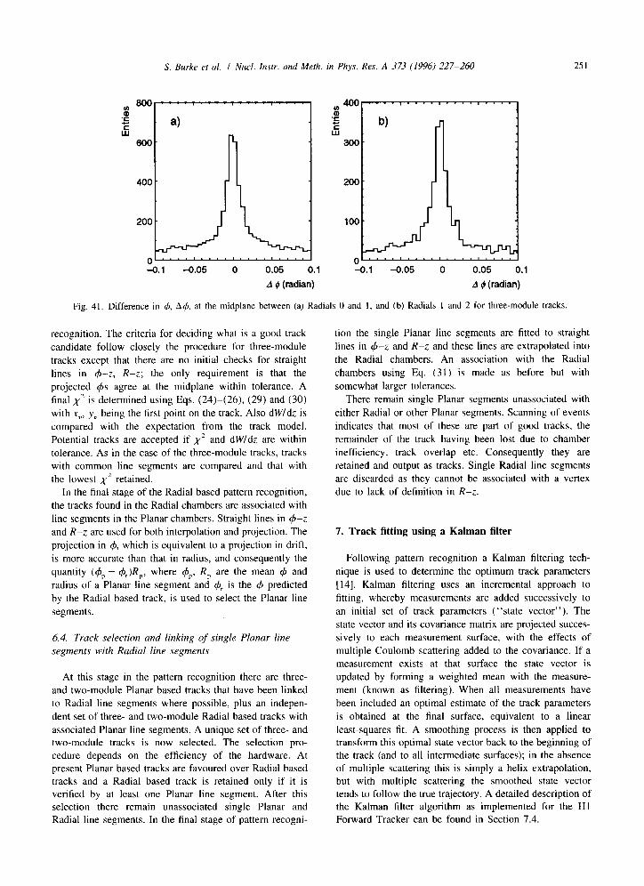
S. Burke et al. I Nucl. Instr. and Meth. in Phys. Res. A 373 (1996) 227-260 251
Fig. 41. Difference in 4, A4, at the midplane between (a) Radials 0 and 1, and (b) Radials 1 and 2 for three-module tracks.
-0.1 -0.05 0 0.05 0.1
A 4 (radian)
zi 400 ‘. . ’ 8.. . . 1 ‘. . ’ 1 ‘. ”
‘C
E b) _I- W
300.
k.1 -0.05 0 0.05 0.1
A 4 (radian)
recognition. The criteria for deciding what is a good track
candidate follow closely the procedure for three-module tracks except that there are no initial checks for straight
lines in +-z, R-z; the only requirement is that the
projected 4s agree at the midplane within tolerance. A
final ,$ is determined using Eqs. (24)-(26). (29) and (30) with .xy, y, being the first point on the track. Also dW/dz is
compared with the expectation from the track model.
Potential tracks are accepted if ,$ and dWldz are within tolerance. As in the case of the three-module tracks, tracks with common line segments are compared and that with
the lowest x2 retained. In the final stage of the Radial based pattern recognition,
the tracks found in the Radial chambers are associated with line segments in the Planar chambers. Straight lines in 4-z
and R-z are used for both interpolation and projection. The
projection in 4, which is equivalent to a projection in drift,
is more accurate than that in radius, and consequently the
quantity (& - qSr)Rp, where $,, RP are the mean r$ and radius of a Planar line segment and $J~ is the 4 predicted
by the Radial based track, is used to select the Planar line
segments.
6.4. Truck selection and linking of single Planar line segments with Radial line segments
At this stage in the pattern recognition there are three-
and two-module Planar based tracks that have been linked to Radial line segments where possible, plus an indepen- dent set of three- and two-module Radial based tracks with
associated Planar line segments. A unique set of three- and two-module tracks is now selected. The selection pro- cedure depends on the efficiency of the hardware. At present Planar based tracks are favoured over Radial based tracks and a Radial based track is retained only if it is verified by at least one Planar line segment. After this selection there remain unassociated single Planar and Radial line segments. In the final stage of pattern recogni-
tion the single Planar line segments are fitted to straight
lines in 9-z and R-z and these lines are extrapolated into
the Radial chambers. An association with the Radial chambers using Eq. (31) is made as before but with
somewhat larger tolerances. There remain single Planar segments unassociated with
either Radial or other Planar segments. Scanning of events
indicates that most of these are part of good tracks, the
remainder of the track having been lost due to chamber inefficiency, track overlap etc. Consequently they are retained and output as tracks. Single Radial line segments are discarded as they cannot be associated with a vertex
due to lack of definition in R-z.
7. Track fitting using a Kalman filter
Following pattern recognition a Kalman filtering tech-
nique is used to determine the optimum track parameters
[14]. Kalman filtering uses an incremental approach to
fitting, whereby measurements are added successively to an initial set of track parameters (“state vector”). The
state vector and its covariance matrix are projected succes- sively to each measurement surface, with the effects of multiple Coulomb scattering added to the covariance. If a measurement exists at that surface the state vector is updated by forming a weighted mean with the measure-
ment (known as filtering). When all measurements have been included an optimal estimate of the track parameters
is obtained at the final surface, equivalent to a linear
least-squares fit. A smoothing process is then applied to transform this optimal state vector back to the beginning of the track (and to all intermediate surfaces); in the absence of multiple scattering this is simply a helix extrapolation, but with multiple scattering the smoothed state vector tends to follow the true trajectory. A detailed description of the Kalman filter algorithm as implemented for the Hl Forward Tracker can be found in Section 7.4.

The Kalman filter is essential in an environment where
multiple Coulomb scattering is significant. The HI For- ward Tracker contains approximately 0.5 radiation lengths
of material, and this is distributed fairly uniformly, pre- cluding the possibility of fitting the track in sections with
scattering allowed between the sections (as is done, for
example, in the H 1 Central Tracker [ 151). Multiple scatter-
ing can give a deviation of several centimetres over the
length of the Tracker for low momentum tracks, and is therefore an important effect.
In a conventional least-squares fit multiple scattering is incorporated by fixing the track parameters at one point, typically the beginning of the track, and then increasing the
errors at each subsequent point to reflect the cumulative amount of scattering along the track. However, these
pseudo-errors are correlated, since they reflect the devia-
tion of the true track from the track model. The track fit therefore requires the inversion of an n X n covariance
matrix, where n is the number of measurements (up to 72
in this case). This is not necessary for the Kalman filter
which follows the true track, with optimal parameter
estimation at every measurement surface.
7. I. Choice of the truck model
The representation of the state vector is chosen to given an approximately linear track model, because the Kalman filter uses a linear approximation for error propagation. It
is also convenient to have a track model with as many
vanishing derivatives in the Jacobian matrix FL (Eq. (33)) as possible, as this allows considerable savings in comput-
ing time for the matrix algebra involved. The geometry of
the Forward Tracker is particularly convenient in this
respect. Since the magnetic field is uniform to better than 2% over the Tracker volume and parallel to the : axis the
equation of motion is close to a helix, which gives a simple propagation from one z plane to another.
The representation used is (x, .v, q/p, tan 6’. 4; :) (i.e. : is fixed for each measurement surface), with the direction of the momentum vector, p, defined by B and r$ in spherical polar coordinates. The main nonlinearity is in the dependence of x and v on 4: 0 and q/p are constants of
the motion, and 4 increases linearly with ;. proportional to ql(p cos 0). First-order corrections to the track model are
made for components of the field transverse to the z axis and for changes in the field as a function of position, but it is not necessary to include these effects in the calculation of the Jacobian F,.
7.2. Point rejection
In a conventional fit it can be difficult to identify points which do not belong to the track, because any deviations become masked by multiple scattering, which can be much larger than the resolution on the points. With a Kalman filter this masking does not happen, and in addition
measurements can easily be added or removed during the fitting process without refitting the entire track each time.
The mechanism for the addition of a new point during
smoothing is simply to take a weighted mean of the
measurement with the smoothed vector. To remove a point requires the inverse of this process, which is equivalent to
the standard filter with a negative measurement covariance.
After either of these the filtered and smoothed vectors at
planes before this point are incorrect. but smoothing can continue with the new state vector without updating these.
If the vector is only required at one end of the detector no more need be done, but otherwise it is necessary to restart the filter from the first altered point, and smooth back to
this point. Further points may be added or removed in this
process. and the procedure can then be iterated. This facility is not a substitute for good pattern recogni-
tion. Although the Kalman filter can reject points which do
not belong to the track this relies on the litted track being a
good approximation to the true track. The pattern recogni- tion should provide a list of points and a state vector
which, when extrapolated, goes within a reasonable dis-
tance (typically a few millimetres) of the points.
7.3. Removal of the initial state L’ector
The Kalman filter requires a ‘*starting vector”, which has to be provided by the pattern recognition. Ideally this should be assigned large errors to avoid biasing the fit. but
in practice a compromise must be made. The reason for
this is that the Kalman filter uses linear error propagation. and therefore the state vector must be kept sufficiently
close to the true track that a linear approximation is
acceptable (i.e. a first order Taylor expansion of the track
propagation equation (Eq. (34)) about the fitted state vector should be an acceptable approximation). In practice
assignment of errors to the starting vector which are about an order of magnitude larger than those expected after the fit gives little bias while maintaining the stability of the fit.
If necessary it is possible to remove the influence of the starting vector by treating it as a virtual measurement that can be removed as described in the previous Section. In the
simplest case, having filtered from the start of the Tracker to the end and smoothed back to the start. the initial vector
can be removed to give an unbiased result. However. this
does not update the results at other planes, and the smoother is not reversible as is obvious from Eq. (34). A more sophisticated procedure is therefore needed if the unbiased result is required at more than just one end of the detector. This is achieved by starting the filter at a point part way along a track, and processing it in two sections. The filter first runs over one part and then smoothes back to the starting plane. The initial state vector is then removed. giving a state vector which contains information from the first section of the track. This is then projected into the other section, where it acts as a new initial state vector. Filtering and smoothing then proceed in the reverse

S. Burke et al. I Nucl. Insrr. and Meth. in Phys. Res. A 373 (1996) Z’7-260 253
direction in that section. At this point the smoothed vector
contains the full information from all measurements, with
no influence from the initial state vector. The starting vector at that point is then removed, giving a vector with information from the second part of the track only. This is
then projected back to the first section. and the filter/ smoother is rerun over this section. This gives the desired result of a state vector at all points with the information
from all measurements, but without any influence from the starting vector and without having to process the whole
track twice.
7.4. Technical description
The general principles of Kalman filtering as applied to track fitting are given in Ref. [ 141, and the notation of that
paper will be followed here. More details, applying in particular to the context of the DELPHI experiment, can be found in Ref. [16]. However, the expressions published in
the above papers have been reformulated to optimise computing efficiency, stability and clarity. This reformula-
tion, as described below, is in some cases completely
general and in others depends upon specific properties of
the HI FTD, but has been found essential in order to achieve the reliability and speed required by mass-pro-
duction event reconstruction.
A state vector (with 5 dimensions for a track fit) is
written as ~1 (lower case variables denote vectors, and upper case denotes a matrix), where k is the surface (plane) index and the value incorporates information up to plane i. The usual cases are ,Y: ’ (or ..r: + , ) for a projected vector,
x: for a filtered vector and ,Y; for a smoothed vector (n is the total number of measurements). The covariance of .Y is
similarly written as Cl. In the following .x: and C’: are written as xk and C,, respectively. The track model (which
projects a state vector from k to k + 1) is given by a
function ji(x,), and Fk is the Jacobian matrix:
(33)
where the derivatives are evaluated at xI. Measurements are related to the state vector via mk = H,x, (where the dimensions of m, and x, are generally different). The measurement covariance is denoted by V, = CL’, and the additional covariance on the state vector due to multiple scattering between planes k and k + 1 by Qk.
The three main steps are projection, filtering and smoothing. These are given in Ref. [ 141 as follows:
!. XI+, =f,(x,)
c:+, = F,C,F: + Q, ;
xI; = C, [(C: I )- ‘xi ’ + HTG,m,]
C, = [(C;-‘,-’ + H:G,HJ’ ;
(projection)
(filtering)
x; =xI +A,(x;+, -x;+,)
C; = C, +A&‘;+, - C;+,)A;
A, = C,F:(C:+, )-’ (smoothing)
(34)
The projection step is straightforward; application of the track model to x. and linear error propagation for C. The
filtering step is also simple, being a weighted mean of the
projected vector with the measurement. However, the
formulation given above contains two inversions of 5 X 5 matrices, and this can be simplified:
X~ = [I + Cf-‘H:G,HJ’x;~’ + C,H:G,m,
C, = [1 + C;~‘H;G,H,]~‘C;~’ (35)
which only involves one inversion. Also, the expression for xp is of the form
xp = W,.x-’ + W>H:m,, (36)
where the weight matrices W, and W, (with W2 = C,H:G,H,) satisfy W, + W, = I; Eq. (36) can therefore be
re-expressed as
xI = Him, + W,(x-’ - H;m,), (37)
which reduces the number of matrix multiplications.
Another major improvement can be made to the filter
equations. The measurements are always space points, and the measurement covariance is therefore 2 X 2 in general (even for Planars the matrix will effectively be 2 X 2 after rotation into (x, y) space, unless the wire is along the x or y
axis). The matrix to be inverted is therefore much simpler
than a general 5 X 5 matrix, and can be inverted ana- lytically (it has two columns of arbitrary elements, with the
remaining diagonal elements being unity and other ele-
ments zero).
A further improvement can be obtained for Planars by
factorising the transformation matrix H out of the inver- sion. Define H’ as the equivalent 5 X 5 rotation matrix:
Then,
C, = HiT[l + H;C;-‘H;TG;]m’H;C;-’ , (39)
where Gi is a 5 X 5 matrix with the inverse of the measurement error in the (I, I) element, and zero else- where. The matrix to be inverted then has one column of arbitrary elements, unit diagonal elements elsewhere and is zero otherwise, and is consequently easy to invert.
The smoothing equations given above are not transpar-

254 S. Burke et al. I NW/. lnstr. and Meth. in Phxs. Res. A 37.1 (1996) .?.?7--760
ent, and can be improved in both clarity and efficiency. Some manipulation gives the equivalent formulation
,Y;I =f,‘(X;+, + w&+, -x’;+,])
C; = A,C;+ !A; + C,( 1 - F;A,7) (40)
= A,C;+,A; + C,F:W;F,“-
= A,C;+,A: + F&A;
where A, =F,‘(l - W,) and W, = Q,(Ci+,)-‘. In the first line, F,’ has been replaced by f,‘. which is
the full inverse track transformation, rather than a linear- ised approximation; this gives a much better behaviour for the smoother. The weight matrix W, is essentially the ratio
of the multiple scattering error to the total projected error, and is therefore zero if there is no multiple scattering. In this case, smoothing is just equivalent to a reverse helix
transformation. In the presence of multiple scattering, the
effect is to adjust the smoothed state vector at k + 1 by the difference between the projected and smoothed vectors at
k + 1, weighted by W,. which gives an estimate of the amount by which the track actually scattered between k
and k + I. This adjusted vector is then projected back
using the inverse transformation. The expressions for the smoothed covariance are some-
what less transparent. In the absence of multiple scattering
this again reduces to linear error propagation. The equiva- lent expressions given have a somewhat different be-
haviour, in that the second term of the second and third expressions manifestly vanishes as Q, + 0, whereas that in the first expression relies on a cancellation. The third
expression is the one currently implemented, as it involves
fewer matrix multiplications. It is, however, not evidently
well-behaved if the multiple scattering is large, since the covariance should tend towards C,, and this relies on a
complex cancellation. This behaviour is possessed explicit-
ly by the first two expressions. This would suggest that the
second expression may be preferable in spite of the additional computation, and this question may require
further investigation. A further issue is whether FL in the smoother (Eq. (40))
should be the same as that used in projection, or re- evaluated at the smoothed point. The most natural solution
would appear to be the latter. In any case, in expressions
involving both F, and F, ’ these must be exact inverses to give the correct asymptotic behaviour, and an extra matrix inversion is therefore required. This again indicates the use of the third of the above expressions for the smoothed covariance, as it only involves F;’ which is readily available from the inverse track transformation applied to the smoothed state vector. Conversely Q, is not re-evalu- ated from the smoothed state vector, as the weight matrix W, compares Qk with the projected covariance, which includes multiple scattering calculated from the projected vector.
It should be noted that a matrix inversion is now only required if there is multiple scattering, and there is
generally a large computational saving if multiple scatter- ing can be neglected between any two planes.
7.5. Code optimisation
Various techniques have been used to increase the execution speed of the code. The two main methods are the
expansion of matrix multiplication in-line and the use of
the known properties of various matrices. These include the symmetry of covariance matrices, that multiple scatter- ing does not change y/p, that the Jacobian matrix F, has
unit diagonal elements, that q/p and 0 are constants of the motion and that changes in the momentum vector direction are independent of small changes in position. The latter
two assumptions are true only if deviations from the
nominal magnetic field can be neglected over each step of the Kalman filter, but this is a reasonable assumption.
For track extrapolation the track model is approximated
wherever possible, either with a straight line or with
first-order approximations for changes in angle. Small- angle approximations are also made where possible for the
evaluation of trigonometric functions. Multiple scattering is neglected within a drift cell. as it entails a substantial amount of calculation.
This optimisation process has been essential to allow the
Kalman filter technique to be used; the cumulative effect of all optimisations is to decrease the computing time
needed by roughly two order of magnitude from a straight- forward implementation, to a point where the Kalman filter
accounts for about 20% of the computing time taken by the
Forward Tracker reconstruction. After optimisation most
time is spend in the projection of the state vector from one
plane to the next, and the time is therefore roughly proportional to the number of measurements.
The increase in time if point rejection is used is unpredictable. The time to remove each point is negligible, but it is then necessary to perform another iteration of the whole fit for those planes which need updating; this time is independent of the number of points removed, but depends on the position of the last point removed, since points
before this do not need to be updated. On average this results in about a 50% increase in computing time.
The main time overhead for the removal of the initial state vector is that the first part of the Tracker is filtered and smoothed twice. It is therefore desirable to have this section as small as possible. The main constraint is that after the removal of the initial vector. enough measure- ments must have been added to give errors sufficiently small that the filter remains stable. If points are added or rejected in the second pass over the first section this invalidates the result in the other section, so this has to be repeated.

S. Burke et al. I Nucl. lnstr. and Meth. in Phvs. Res. A 373 (1996) 227-260 255
8. Alignment of the Forward Tracker
8.1. Data sample Planar Orientation
The internal alignment of the Forward Track Detector uses a sample of cosmic ray tracks recorded in zero magnetic field. These tracks were selected using a scin- tillator trigger that required the track to intersect the interaction region and to traverse all three Supermodules. Data are corrected for the time offsets measured for each
individual cell using artificially generated test pulses. A special form of pattern recognition has been developed
which exploits the fact that the tracks are straight lines. Radial Module
8.2. Planar pattern recognition for alignment data Fig. 42. Definition of alignment parameters relative to the nomi-
nal values.
The nomenclature used in this Section is the same as that in Section 6.2. The four digitisations which form the
best straight line for each orientation are found. All such digitisations (up to 36) are then fitted to a straight line. There are many occasions where track related noise and the intrinsic resolution of the data cause wrong digitisa- tions to be chosen. A procedure for removing bad digitisa-
tions and adding in good ones is therefore implemented. Any of the digitisations contributing more than 100 to x’
or more than three and a half times the average $/degree- of-freedom are noted. The worst two of these are removed
from the track and the track is refitted. At wire planes which do not have a hit associated with the track the
closest hit is attached if it is within a given distance of the
track. The tracks are then refitted to give new track parameters and the procedure repeated until no further hits
are removed or added. Checks are made to ensure the procedure does not loop; if it does the iteration is termi- nated. Scanning has verified that this method is efficient at
correctly identifying hits and tracks.
8.3. Alignment of the Planar chambers
Tracks which satisfy the above criteria are corrected for the following. l Time of flight. A correction is made to the drift time at
each plane using the fitted track parameters and assum- ing the particle’is travelling at the speed of light in the
direction giving the smaller x’. l Track angle effect. This is calculated from the fitted
track parameters. The correction described in Section 4.1 is parametrised by a single variable d. The fitted value of
d agrees well with that obtained from theoretical calcu- lations (-0.5 cm).
l Propagation time along a sense wire. The propagation
speed is fitted and found to be close to the speed of light. Having made these individual corrections for each track
This sample of tracks must however be treated with some caution as low momentum tracks have noticeable
effects from multiple scattering. This causes them to have either a poor fit or few digitisations associated. To ensure a
good sample, tracks are required to have an associated
planar digitisation on at least 20 of the 36 planes and a
x’ < 700. Each event has also been scanned to ensure that the track is a sensible candidate. Given these requirements a sample of just over 500 clean tracks remains.
a x2 is calculated for a global fit to all tracks. Before freeing the alignment parameters a global t, and drift
velocity are fitted. Two additional parameters are fitted which describe any deviation from the nominal wire stagger and wire spacing within a cell. In the fit one
orientation is fixed in space and each of the remaining
eight orientations has AZ, Acr and AW fitted (see Fig. 42)
where AZ is a translation along the z axis, ALY is a rotation
about the z axis and AW is a translation perpendicular to the wires. The W coordinate of an extra orientation is fixed in order to uniquely specify the position of the RD. The
Table 7 Planar alignment parameters with orientation 3 and the W coordinate of orientation 8 fixed at their nominal values. together with an estimate
of the errors
Orientation Error
0 1 2 3 4 5 6 I 8
A(Y [mrad] -0.37 -0.29 0.13 0 0.15 0.10 0.08 0.10 0.16 0.15
AW Mnl -8 55 57 0 102 -102 106 15 0 50
AZ Mnl 628 416 518 0 -751 207 -167 -192 28 500

256 S. Burke et al. I Nucl. Instr. und Meth. in Phw. Res. A 373 (1996) .?27-260
results have been tested for stability by changing the orientation that is fixed and are given. along with an estimate of the errors, in Table 7. None of the resulting
corrections have a significant effect on the track recon- struction with the exception of the rotation of orientations 0 and I.
8.4. Alignment of the Radial chambers
The next step is to align the Radial chambers with
respect to the Planar chambers. Digitisations from the
Radial chambers are parametrised by their drift distance
and the wire-angle in the x-y plane, ignoring any in- formation from charge division. This makes Radial data
similar to Planar data, with each Radial digitisation defining a line in space. The digitisations closest to the track defined by the Planars and within 0.5 cm of it are associated with the track. As it is not possible to determine
the Radial drift velocity and t,, using Radial data alone, a
fit for these parameters is first made for the Radial data with respect to the track defined by the Planars. The Radial
track angle effect is then calibrated by fitting one free parameter which is subsequently fixed. In the final fit the
Planar and Radial data are fitted simultaneously with free parameters Aa, A.r, A): and Az for each of the three Radial
chambers (Fig. 42), but with the Planar alignment parame-
ters fixed. The results are shown in Table 8. None of the
resulting corrections have a significant effect on the track reconstruction.
9. Performance
The performance of the reconstruction code has been assessed mainly by using a Monte Carlo simulation, with cross-checks from real data. The simulation will be briefly
described, followed by the results of various measures of
performance.
9. I. Simulation
The HI simulation program uses the GEANT frame- work [ 171 to track particles through the detector. The GEANT description of the Forward Tracker treats each
Planar drift cell as a single volume; for the Radials, each
Table 8
Radial alignment parameters with the Planar alignment parameters
fixed at the values given in Table 7, together with an estimate of
the errors
Module
Aru [mrad]
hx lt@ AY [Km1 AZ [@ml
0 I 2 Error
0.26 0.24 0.31 0.20
-192 166 -92 70
-376 -120 131 70
-309 405 269 500
chamber is a single volume (i.e. the cathode planes are not
included). The GEANT tracking code outputs a direction and momentum for each particle at the entrance and exit point of each volume. This is followed by a simulation of the digitisation process. A full simulation of the drift of charge in the chamber gas, followed by the response of the
analogue electronics and the QT code, is impractical, so a parametrised simulation is used. This begins with the mean
energy loss as a function of momentum and particle type.
Landau fluctuations in the energy loss are simulated according to the GEANT routine GLANDZ. This energy is
then scaled to give approximately the same average Q
value as seen in real data. For the Radials, the charge is
split according to the inverse of the charge division algorithm used in reconstruction (see Section 4.3.2) with equal preamplifier gains. Hits are removed using an efficiency derived from real data, but without including any correlations with the energy deposited (see Table 6).
The limits on acceptance due to the Lorentz angle are included.
True random noise is very rare (around 1 hit per event). However, analysis of data shows that there is a significant
background of track-related noise hits within a few mil-
limetres of the true hits. These are simulated using parametrised distributions derived from data.
The detailed fluctuations in the FADC pulse shape are
not currently well understood. Consequently. a standard (triangular) pulse is used as input to an emulation of the QT algorithm (Section 3), with various pulse-shape depen- dent effects added empirically. These include the two-track
resolution. parametrised as a linear rise from 0% separation efficiency at 1 mm to 100% at 2.8 mm; the drift time of a group of hits when unresolved is taken as a charge-
weighted average for the Planars and the time of the largest pulse for the Radials. The charge integral for the Radials is truncated at the start of the following hit if it is
closer than the normal integration length.
The drift and charge measurements are then smeared
using empirical resolutions, including the variation of drift resolution with drift distance (see Section 4). The smearing is increased if there is a close preceding hit, dependent on both the hit separation and the relative pulse heights. If the smeared charge is too small the hit is discarded. A linear distance-to-time relation is used, with a similar drift
velocity to the average in real data. The simulation described above gives a generally
reasonable match with the data at the segment level. However, there is evidence for a correlated loss of hits in a
Table 9
Probability of removing all hits from a given track in one drift cell
for Radials (R) and Planars (P)
Supermodule
Probability (R)
Probability (P)
0 I 2 0.05 0.05 0.25
0.07 0.08 0.09

S. Burke et ul. I Nucl. Instr. und Mrth in Phys. Res. A 372 (19961 227-260 251
Drift Residuals (cm)
-0.2 -0.1 0 0.1 0.2
Dtift Residuals (cm)
Fig. 43. Single segment drift residuals for both data and Monte Carlo for (a) Planars and (b) Radials.
drift cell at an appreciable rate, due either to timing
problems, to breakdown or to other problems within the cell. This loss is estimated from the distribution (Table 10) of segments attached to individual tracks and is given in Table 9. The 25% loss in Radial Supermodule 2 can be attributed to the high hit density resulting from interactions
in the collimator (Section 2).
9.2. Comparison between simulated and real data
Neutral current deep inelastic events have been gener- ated by the LEPTO [ 181 program, and after simulation and
reconstruction have been selected to have significant
hadronic activity, a large proportion of which is in the FTD. The primary track multiplicity is -10 to 15. In
addition there are 40 to 60 mainly low momentum secondary tracks, a substantial number of which originate from the collimator and only penetrate the last Super- module. The simulation used the efficiences for the 1993
data-taking period (Table 6). The output of the simulation has been compared in
detail with real data with the same selection, using measures which are insensitive to the underlying physics
processes. The primary comparison is at the segment finding level; Fig. 43 shows the drift residuals for single
segments for both simulated and real data. The agreement is good. The radius reconstruction depends on the details of charge fluctuations, which are not well understood and not well reproduced by the Monte Carlo, but the track
reconstruction does not depend significantly on the radius measurement.
Fig. 44 shows the distributions of the numbers of hits on Planar and Radial segments, which indicate that the hit finding efficiency is approximately correct. The data distribution for the Radials is broader than the Monte Carlo due to summing over runs with differing efficiencies. Fig. 45 shows the xz probability distribution for the overall
0 6 12 0 6 12 Number of hits on segment Number of hits on segment
Fig. 44. Number of hits on single segments for both data and
Monte Carlo for (a) Planars and (b) Radials.
track fit. Although the fraction of tracks in the low- probability bin is sensitive to pattern recognition errors,
and in particular to the presence of track-related noise hits, the agreement between Monte Carlo and data is excellent.
Table IO shows the distribution of the number of Planar
0 0.2 0.4 0.6 0.6 1
f Probability
Fig. 45. x2 probability distribution for the overall track fit.

258 S. Burke et al. I Nucl. Instr. und Meth. in Phys. Rus. A 37.1 (1996) 227-260
Table 10 The percentage of tracks in data (Monte Carlo) with different numbers of Radial (R) or Planar (P) segments attached. All tracks are required
to have at least one Planar segment attached
OR IR ?R 3R Any R
1P 48.5 (35.2) 18.4 (23.1) 9.4 ( 12.4) 2.1 (2.5) 78.4 (73.2) 2P 3.7 (4.2) 6.2 (8.5) 4.9 (7.0) 2.3 (2.3) 17.1 (22.0) 3P 0.7 (0.7) 1.5 (1.8) 1.5 (1.7) 0.8 (0.6) 4.5 (4.8) Any P 52.9 (40.1) 26.1 (33.4) 15.8(21.1) 5.2 (5.4) 100.0 (100.0)
and Radial segments attached to tracks. The distributions
are influenced by the underlying physics processes. Never-
theless there is good agreement between data and Monte Carlo, indicating that the hit and cell efficiencies are
reasonably accurate, and that the resolutions lead to
comparable segment linking efficiencies.
It can be seen from the above figures and tables that the simulation gives an excellent description of the real data at
the hit, segment and track level. The simulation gives a sufficiently good match to allow reliable figures on recon-
struction performance to be determined.
9.3. Performance
Important performance criteria are the track finding
efficiency as a function of angle and momentum (par-
ticularly for primary tracks), and the momentum and angular resolution. These have been evaluated for neutral
current events using the simulated data described above.
Fig. 46 shows the track finding efficiency as a function of pseudorapidity for primary tracks with momentum above 0.5 GeV/c. The dotted line shows the corresponding
efficiency for the HI Central Tracker. The comparison is with that Monte Carlo track which contributes the largest
number of hits to the pattern recognised track. The variation of efficiency with angle is determined by the
Forward Tracker acceptance, while the main limiting factor on the maximum efficiency is the correlated loss of
3 3.5
Pseudorapidity
Fig. 46. Track finding efficiency as a function of pseudorapidity
for primary tracks with momentum above 0.5 GeVlc. The dotted
line shows the corresponding efficiency for the HI Central
Tracker.
all data in a drift cell (Table 9). The figure shows that the
efficiency rises from 50% at 6” to 80% at 9”. The Tracker
increases the range of track measurements in the forward
direction by one unit of pseudorapidity. Fig. 47 shows the efficiency as a function of momentum,
p, for primary tracks with 9” < 0 < 18” (which is the range
over which the efficiency is independent of 0). It can be seen that the efficiency is essentially independent of
momentum above 0.5 GeV/c. The fraction of tracks found more than once, i.e. split
into more than one piece. is less than I%, and is roughly independent of angle and momentum. For 70% of recon-
structed tracks the fraction of hits which are correct is
greater than 80%. Another way of assessing the track finding efficiency is
to look at events with tracks in other tracking detectors. and scan by eye to see whether corresponding tracks are
seen in the Forward Tracker. This has been done for
samples of a few hundred events, for low track multip- licities, and in a limited angular range. It gives results in
agreement with those from Monte Carlo data. Fig. 48 shows the distributions of A( y/p), the difference
between the reconstructed and true q/p, for tracks with and without a fit to the primary interaction vertex. In each case
the distributions are shown for 0.5 <p < I GeV/c, I <p <
3 GeV/c and p > 3 GeVlc. Table II gives the resolutions in q/p from the fits shown in Fig. 48 [ 191. The momentum
dependence is due to multiple scattering. It can be seen
that the inclusion of the vertex improves the momentum resolution by about a factor of 2 for momenta above 3 GeV/c. The polar angular resolution is 0.2 mrad for
or 0.3 1 3 10
p (GeV/c)
Fig. 47. Efficiency as a function of p for primary tracks with
9”<8<18”.

S. Burke et al. I Nucl. lnstr. and Meth. in Phys. Res. A 373 (1996) 227-260 259
Table 1 I Resolution in q/p (%lGeVlc) for the FTD
Momentum range 0.5 < p < 1 GeV/c l<p<3GeVlc p > 3 GeVlc
Tracks without vertex 19.9 7.9 5.4
Tracks with vertex 14.1 5.6 2.7
-0.5 -0.4 -0.3 -0.2 -0.1 0 0.1 0.2 0.3 0.4 0.5 Abdol IIGeVlckll
‘E
;_ d P m 0 ‘5 6
-0.5 -0.4 a.3 -0.2 -0.1 0 0.1 0.2 0.3 0.4 0.5
1 .s m .; E
-0.5 -0.4 -0.3 -0.2 -0.1 0 0.1 0.2 0.3 0.4 0.5 AW’) UGeVW’)
Fig. 48. A(qlp) for tracks with and without a fit to the primary
vertex for (a) 0.5 <p < 1 GeV/c, (b) 1 < p < 3 GeV/c and (c)
p > 3 GeVlc. The solid histograms are for primary tracks with a
vertex fit, the dashed for all tracks, but without a vertex fit. The
fitted curves are generalised Breit-Wigners [ 191.
three-module, high momentum tracks and better than
1 mrad for the majority of tracks.
10. Summary
This paper has described the reconstruction of tracks in a detector that operates in an environment made complex by the high hit density from proton fragmentation, and the
large number of photon conversions and other secondary interactions in the end wall of the Central Tracker and the nearby collimator.
The procedures used to analyse the FADC pulses and
determine the drift velocities, timing offsets, resolutions and efficiencies of the chambers have been discussed. A
technique has been developed for alignment of the multi- detector system.
The pattern recognition and track fitting procedures that have been optimised for the mix of Radial and Planar chambers of the Hl Forward Track Detector have been described in detail. Monte Carlo studies, supplemented by visual scanning, have shown that in spite of the complexity of the events, tracks are found with an efficiency -80%
over a wide range of the acceptance. The Tracker extends
the range of track measurement in the forward direction by
one unit of pseudorapidity.
Acknowledgements
We wish to thank the staff at the UK Universities and RAL, who have been responsible for the design, construc-
tion and maintenance of the FTD, and whose efforts have
provided the foundation for the work described in this paper. The hospitality extended to us by the staff and
directorate at DESY, leading up to and during the first
years of HERA operation, has been greatly appreciated. We thank the funding agencies for their support and the Hl
experiment and the UK PPARC (formerly SERC), in
particular, for financial support of the FfD project. We also wish to thank the staff of the Cosener’s House for their excellent hospitality which provided an environment that greatly facilitated the writing of this paper. Finally our
thanks for careful typing and constructively critical reading of this paper go respectively to Miss Ann Richardson of
the Rutherford Appleton Laboratory and to Dr. David
Newton of the University of Lancaster.
References
[II
121
131
f41
[51
[61
f71
VI
W. Buchmiiller and G. Ingelman (eds.), Proc. Workshop on
Physics at HERA, DESY, vol. 1, October 29-30, 1991.
The HI Detector at HERA, Hl Collaboration. DESY 93-103
(July 1993).
Technical Proposal for the HI Detector. Hl Collaboration,
DESY (March 1986).
The techniques used in electron identification are described
in more detail in H. Grassier et al., Nucl. Instr. and Meth. A
323 (1992) 401.
The most detailed (although not necessarily up-to-date)
description of the Forward Tracker may be found in The Hl
Forward Tracker Description and Status, Hl FTD Group, DESY Hl-TR-205 (October 1987).
See for example G.A. Beck et al.. Nucl. Instr. and Meth. A
283 (1989) 471;
H. Grassier et al., Nucl. Instr. and Meth. A 283 (1989) 622;
H. Grassier et al.. Nucl. Instr. and Meth. A 3 10 (1991) 535;
J.M. Bailey et al.. Nucl. Instr. and Meth. A 323 (1992) 184.
D. Schaile, 0. Schaile and J. Schwarz, Nucl. Instr. and Meth.
A 242 (1986) 247.
S.M. Tkaczyk et al.. Nucl. Instr. and Meth. A 270 (1988)
373.

260 S. Burke et ~1. / Nuc.1. Irtstr. crrtd Mrtlt. in Plr~s. Rrs. A -77.7 (199h) 1777-X)
[9] D.P.C. Sankey. Ph.D. thesis. University of Liverpool. RALT-
115. 1990.
[IO] V. Radeka and P. Rehak. IEEE Trans. Nucl. Sci. NS-26
(1979) 225.
[I I] F. Sauli. CERN 77-09 ( 1977).
[I21 J.V Morris, RAL report, to be published.
[I31 R. Veenhof, CERN User Guide W5050, URL (http://con-
sult.cem.ch/writeup/garfield/main.html).
1141 R. Friiwirth, Nucl. Instr. and Meth. A 262 ( 1987) 447.
[ 151 V. Blobel, private communication.
[I61 R. Friiwirth, HEPHY-PUB 516/88,Vienna (1988);
R. Friiwirth et al.. HEPHY-PUB 578193. Vienna (1993).
1171 CERN Program Library Ql23. URL (http://wwwcn.cem.ch/
asdoc/geant/GEANTMAIN.html).
1181 G. Ingelman, Proc. Workshop on Physics at HERA, eda. W.
Buchmiiller and G. Ingelman. DESY. Vol. 3. October 39930,
1991. p. 1366.
[ 191 We define the generalised Breit-Wigner distribution as
G(.r) = a I t [_ (
+/Li _ ll(nt’>l>~‘~,
The function has half-width at half height equal to y and
approaches a simple Breit-Wigner as p approaches I or a
Gaussian as it tends to infinity. The values in Table I I are
r(2 In 2)-l”. which corresponds to v for a Gaussian.