2d least squares matching applied to piv challenge...

16th Int Symp on Applications of Laser Techniques to Fluid Mechanics Lisbon, Portugal, 09-12 July, 2012

2D Least Squares Matching applied to PIV Challenge data (Part 1)

J. Kitzhofer1*, F. G. Ergin2, V. Jaunet2

1: Dantec Dynamics GmbH, Ulm, Germany

2: Dantec Dynamics A/S, Skovlunde, Denmark * Corresponding author: [email protected]

Abstract 2D Least Squares Matching (2D LSM) technique is applied to the PIV challenge test data in order to extend the knowledge about the application of LSM as an alternative to cross-correlation based algorithms. Despite its distinct advantages, only few PIV experiments are evaluated by Least Squares Matching. Detailed knowledge on LSM’s limits and potential improvements is not yet established. With this in mind, the objective of this paper is to apply 2D LSM algorithm to selected PIV challenge data sets [5]. The implemented 2D LSM algorithm uses 2D Cross Correlation as initial guess for 2D LSM. This increases stability and decreases processing time. The least squares matching algorithm is applied by changing boundary conditions, interrogation area size or number of iterations and varying velocity fields. 1. Introduction 2D Least Squares Matching (LSM) is not a recent technique in obtaining velocity fields using image-based data. It was already applied in 1994 for volumetric Laser Induced Fluorescence (LIF) [1], in 1996 for tracking 2D particle ensembles (PTV) [2] and was compared to several correlation-based PIV evaluation algorithms in 2000 [3]. LSM is a gray-level tracking technique, which performs translation, deformation and rotation of the interrogation area, where Cross Correlation (CC) only performs translation. Deforming-window techniques mimicking rotation and shear decrease the uncertainty in cross-correlation based algorithms. In LSM, the movement of a fluid element, captured within two successive time steps, is tracked in an iterative least squares adjustment procedure, where the gray values of the interrogation area at time step one are transformed into the gray values of the interrogation area at time step two. Due to its iterative nature and its non-applicability to FFT [3], the LSM technique is subject to longer computation times and therefore received less attention compared to 2D Cross Correlation. Nevertheless, the availability of high performance computers and the inclusion of 2D CC as an initial step to LSM have diminished this limitation. Processing times are nowadays acceptable and comparable to that of CC based multi-grid, multi-pass algorithms with deforming windows. This makes 2D LSM an attractive alternative for the measurement of Eulerian velocity fields. Advantages of LSM are known and reported in literature, see Tokumaru and Dimotakis [4] or Gui and Merzkirch [3]. Advantages are found in adaptivity to discrete particle data as well as continuous scalar representations. Furthermore, the authors claim that systematic errors inherent to FFT-based 2D CC algorithms like low sampling are not apparent in 2D LSM. This increases the accuracy of the measured velocity field. Despite its distinct advantages, only few PIV experiments are evaluated by LSM. Detailed knowledge on LSM’s limits and potential improvements is not yet established. With this in mind, the objective of this paper is to apply 2D LSM algorithm to selected PIV challenge data sets [5]. The PIV challenge data is designed by the fluid mechanics community to test different aspects of the PIV analysis. The results are documented in detail in several review papers. [5]. In total, three PIV challenges have been performed. The published data contains real and simulated particle images of different flows with variable particle density and size; suitable for the analysis with 2D PIV, 2D PTV and stereoscopic PIV techniques.

- 1 -


This paper focuses on datasets of PIV challenge 1 and 2, namely (Challenge 1 Case A, Case B, Case C and Challenge 2 Case A and Case B). The analysis of the rest of the data is subject of another paper, which will be presented at the PIV 2013 in Delft, Netherlands. 2. Selection of PIV Challenge Dataset In total three International PIV Challenges have been performed. Each challenge focused on a different aspect of the PIV analysis [5, 6, 7]. In the following, the data, which is open to public, is briefly described. PIV challenge 1 (namely “Challenge on PIV image evaluation and post processing algorithms”) contained one double image of a strong vortex flow (Case A), one double image of simulated strong vortex flow (Case B), one of a real turbine flow containing strong reflections (Case C) and one double image of a simulated shear flow (Case E) [5]. PIV challenge 2 (namely “Challenges for the turbulent structure analysis and Camera characteristics”) focused more on a statistical description of the results including series of double images. 100 double images of a real jet flow (Case A), a simulation of a turbulent channel flow (Case B) and a real time resolved measurement of the flow on the suction side of an airfoil (Case C) [6] are analyzed. PIV challenge 3 (namely “Assessment of Spatial resolution, Time-resolved PIV and Stereo PIV”) mainly contained images for the detailed analysis of the spatial resolution. Case A contains 4 sets of 100 synthetically generated particle images with varying velocity spectra and spatial frequencies. Case B shows allows the analysis of different signal to noise ratios. Finally, Case C was designed to analyze the application of CC algorithms to real high-speed particle images [7]. The generated data is too much for the analysis in one single paper. Thus, in a first part this paper focuses on the first half of the data, PIV Challenge 1 Case A, B, C and E and PIV Challenge 2 Case A and B. The results of the rest of the data will be presented at an upcoming conference. All data is downloaded from www.pivchallenge.org. 3. Algorithms (Challenge 1 Case A) This chapter describes the algorithms used for the calculation of the velocity field from particle images of PIV Challenge 1 Case A. All velocity fields are obtained from Dantec Dynamics commercial software DynamicStudio V3.30. The tested algorithm is 2D LSM where 2D adaptive Correlation provides the initial condition for the iterations. This chapter describes the implementation of the algorithms Adaptive Correlation, 2D LSM and 2D LSM with adaptive correlation as initial guess. 3.1 2D Adaptive Correlation The principle of Adaptive correlation is an iterative procedure, where a shifted window is used to increase the correlation peak. In an iterative manner, the size of the interrogation area (at positions defined by the estimated translational velocity components) is decreased to fit the particle pattern between the two time steps. Main advantages are decreased in-plane particle dropout, increased dynamic range, and better accuracy in inhomogeneously seeded flows with varying number particle density. A detailed description of the implementation can be found in [8]. Case B form PIV Challenge 1 is a particle image of an experiment performed in a wind tunnel at DNW-LLF by DLR to study the wake vortex formation behind an aircraft. The particle image is characterized by strong gradients in the flow field and by inhomogeneous seeded regions (size and density).

- 2 -

http://www.pivchallenge.org/


The analysis of the double image with Adaptive Correlation is shown in Figure 1. The parameters of the adaptive correlation are chosen to final interrogation area size 32x32 pix² with initially 64x64 pix² and 50 % overlap. No filters or image deformation techniques are applied. Afterwards, a universal outlier detection is applied a described in [9]. In the following all velocity fields are interpolated onto a regular 80 by 64 grid for comparison. The interpolation is performed via a thin plate spline with a radius of 60 and a relaxation of 0.3. No peak-ratio or SNR validation is involved. The resulting velocity field after universal outlier detection is shown in Figure 1. The figure on the left shows the velocity vector field where colours indicate the vector length. The figure on the right shows the magnification of the vortex core. As shown in Figure 1 on the bottom, the cross correlation peak is not dominant in the vortex core, due to insufficient number and visibility of seeding particles [5, 6, 7].

-15

-10

-5

0

5

10

0 200 400 600 800 1000 [pix]

v [p

ix]

Adaptive Correlation clean Adaptive Correlation raw

Fig 1 PIV Challenge 1 Case A: (top left) Velocity vector field calculated by adaptive correlation, universal outlier

detection and interpolation onto a 80x64 grid. (top right) Magnification of the vortex core; color-coding: vector

length with maximum at 12 pix displacement. (bottom) Profile plots velocity component v along x at y=490,

clean: universal outlier detection applied, raw: no universal outlier detection applied 3.2 2D LSM 2D Least Squares Matching is a tracking technique, which performs translation, deformation and rotation of the interrogation area as shown in Figure 2. The main principle of LSM is the application of an affine transformation between two interrogation areas. In addition to the zero order translational velocity components, the affine transformation takes into account first order deformations. The affine transformation is calculated in an iterative manner (least squares matching) until a minimum in gray value difference between two time steps is reached. The implemented algorithm is described in detail in [10]. The extraction of the velocity gradient matrix

- 3 -


is described in [11]. In these articles, it is also shown that the assumption of an affine transformation is sufficient for small deformations (small separation times). One significant advantage of LSM is that the first order deformations of the interrogation area are readily available up to a certain convergence level after each computation. Unfortunately, this is not the case for Cross Correlation, where the deformation of an interrogation area can only be computed from neighbouring velocity vectors using central difference schemes.

Fig 2 (from left to right) translation, rotation, strain, shear Due to its iterative nature and the resulting long processing times compared to Cross Correlation, LSM has fallen behind 2D CC. Nevertheless, increasing computer performance makes the technique applicable to PIV data.

2D LSM 40 iterations 2D LSM 100 iterations

2D LSM with adaptive correlation, 40 iterations

2D LSM with adaptive correlation, 100 iterations

Fig 3 Influence of Cross Correlation as initial guess for 2D LSM with respect to rejected vectors

3.3 2D LSM with Adaptive Correlation All iterative methods require an initial guess for the calculation. In case of PIV data, the initial guess would be a displacement vector for an interrogation region. A good initial guess is estimated in the implemented LSM algorithm by the adaptive correlation. Two main influences are observed: 1) Number of necessary iterations decreases rapidly and as a result 2) number of outliers rapidly decreases. Figure 3 and 4 show the influence of the Correlation as initial guess. The parameters of LSM are chosen to an interrogation area size of 33x33 with 66% overlap and a rather strict convergence level

- 4 -


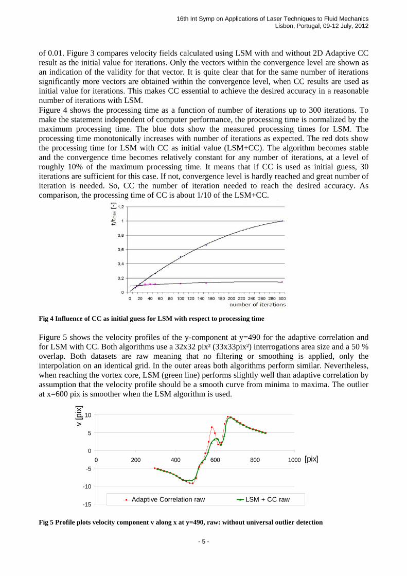
of 0.01. Figure 3 compares velocity fields calculated using LSM with and without 2D Adaptive CC result as the initial value for iterations. Only the vectors within the convergence level are shown as an indication of the validity for that vector. It is quite clear that for the same number of iterations significantly more vectors are obtained within the convergence level, when CC results are used as initial value for iterations. This makes CC essential to achieve the desired accuracy in a reasonable number of iterations with LSM. Figure 4 shows the processing time as a function of number of iterations up to 300 iterations. To make the statement independent of computer performance, the processing time is normalized by the maximum processing time. The blue dots show the measured processing times for LSM. The processing time monotonically increases with number of iterations as expected. The red dots show the processing time for LSM with CC as initial value (LSM+CC). The algorithm becomes stable and the convergence time becomes relatively constant for any number of iterations, at a level of roughly 10% of the maximum processing time. It means that if CC is used as initial guess, 30 iterations are sufficient for this case. If not, convergence level is hardly reached and great number of iteration is needed. So, CC the number of iteration needed to reach the desired accuracy. As comparison, the processing time of CC is about 1/10 of the LSM+CC.

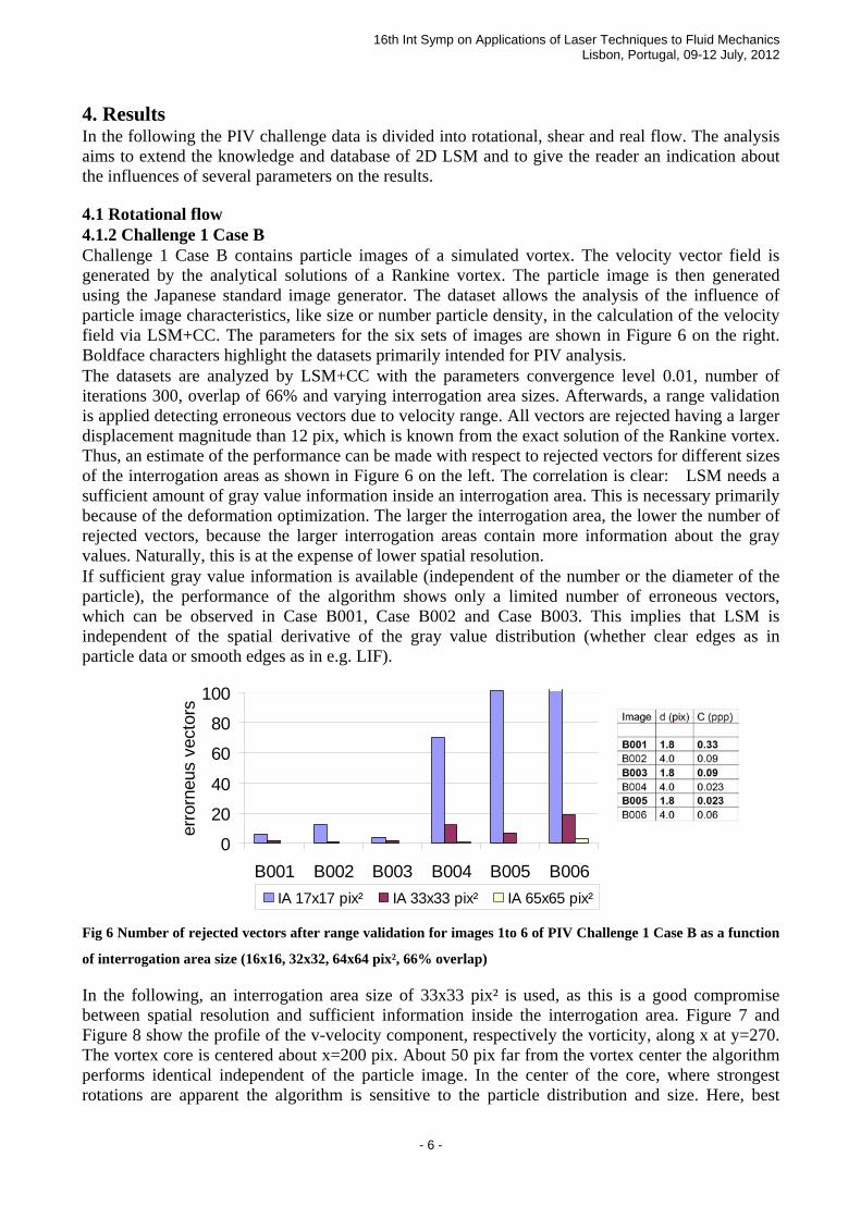
Fig 4 Influence of CC as initial guess for LSM with respect to processing time Figure 5 shows the velocity profiles of the y-component at y=490 for the adaptive correlation and for LSM with CC. Both algorithms use a 32x32 pix² (33x33pix²) interrogations area size and a 50 % overlap. Both datasets are raw meaning that no filtering or smoothing is applied, only the interpolation on an identical grid. In the outer areas both algorithms perform similar. Nevertheless, when reaching the vortex core, LSM (green line) performs slightly well than adaptive correlation by assumption that the velocity profile should be a smooth curve from minima to maxima. The outlier at x=600 pix is smoother when the LSM algorithm is used.

Fig 5 Profile plots velocity component v along x at y=490, raw: without universal outlier detection

-15

-10

-5

0

5

10

0 200 400 600 800 1000 [pix]

v [p

ix]

Adaptive Correlation raw LSM + CC raw

- 5 -


4. Results In the following the PIV challenge data is divided into rotational, shear and real flow. The analysis aims to extend the knowledge and database of 2D LSM and to give the reader an indication about the influences of several parameters on the results. 4.1 Rotational flow 4.1.2 Challenge 1 Case B Challenge 1 Case B contains particle images of a simulated vortex. The velocity vector field is generated by the analytical solutions of a Rankine vortex. The particle image is then generated using the Japanese standard image generator. The dataset allows the analysis of the influence of particle image characteristics, like size or number particle density, in the calculation of the velocity field via LSM+CC. The parameters for the six sets of images are shown in Figure 6 on the right. Boldface characters highlight the datasets primarily intended for PIV analysis. The datasets are analyzed by LSM+CC with the parameters convergence level 0.01, number of iterations 300, overlap of 66% and varying interrogation area sizes. Afterwards, a range validation is applied detecting erroneous vectors due to velocity range. All vectors are rejected having a larger displacement magnitude than 12 pix, which is known from the exact solution of the Rankine vortex. Thus, an estimate of the performance can be made with respect to rejected vectors for different sizes of the interrogation areas as shown in Figure 6 on the left. The correlation is clear: LSM needs a sufficient amount of gray value information inside an interrogation area. This is necessary primarily because of the deformation optimization. The larger the interrogation area, the lower the number of rejected vectors, because the larger interrogation areas contain more information about the gray values. Naturally, this is at the expense of lower spatial resolution. If sufficient gray value information is available (independent of the number or the diameter of the particle), the performance of the algorithm shows only a limited number of erroneous vectors, which can be observed in Case B001, Case B002 and Case B003. This implies that LSM is independent of the spatial derivative of the gray value distribution (whether clear edges as in particle data or smooth edges as in e.g. LIF).

0

20

40

60

80

100

B001 B002 B003 B004 B005 B006

erro

rneu

s ve

ctor

s

IA 17x17 pix² IA 33x33 pix² IA 65x65 pix²

Fig 6 Number of rejected vectors after range validation for images 1to 6 of PIV Challenge 1 Case B as a function

of interrogation area size (16x16, 32x32, 64x64 pix², 66% overlap) In the following, an interrogation area size of 33x33 pix² is used, as this is a good compromise between spatial resolution and sufficient information inside the interrogation area. Figure 7 and Figure 8 show the profile of the v-velocity component, respectively the vorticity, along x at y=270. The vortex core is centered about x=200 pix. About 50 pix far from the vortex center the algorithm performs identical independent of the particle image. In the center of the core, where strongest rotations are apparent the algorithm is sensitive to the particle distribution and size. Here, best

- 6 -


results are observed by B001, which is characterized by a large number of small particles providing displacement information. A comparison of the maximum displacement calculated via LSM with maximum “real” velocity (known from the exact solution, shown as slash dotted line in figure 7), the deviation is in the order of 2-3 pix. This is in line with the order of magnitude for the most advanced CC algorithms described in [5].

Fig 7 PIV Challenge1 Case B: displacement profile for the single double images along x at y=270

The vorticity profile shows a similar pattern in Figure 8. Best results are observed for Case B001, due to the better estimation of the velocity filed. Here, the calculated maximum vorticity matches exactly with the maximum vorticity known from the exact solutions. In contrast to CC based algorithms, which usually perform a low pass filtering showing a smaller estimated value, the LSM algorithm behaves like a high pass filter, which needs further investigation. Nevertheless, the profile is in good agreement independent of the image characteristic, which makes the technique very robust (necessary for real applications).

-15

-10

-5

0

5

10

15

0 100 200 300 400 x [pix]

v [p

ix]

B001 B002 B003 B004 B005 B006

-0,8-0,7-0,6-0,5-0,4-0,3-0,2-0,1

00,1

0 100 200 300 400 500 x [pix]

vorti

city

B001 B002 B003 B004 B005 B006

Fig 8 PIV Challenge1 Case B: vorticity profile for the single double images along x at y=270

- 7 -


4.2 Shear flow 4.2.1 Challenge 1 Case E Challenge 1 Case E consists of a series of numerically generated double images with varying velocity gradients du/dy. Furthermore, a non-uniform illumination is included from left to right (in x-direction). The dataset tests the performance of the LSM algorithm with respect to high shear gradients and its sensitivity to non-uniform illumination. The parameters of the LSM algorithm are set to convergence level 0.01, interrogation area size of 15x15, 33% overlap, 300 iterations, cross correlation as initial guess, range validation and following grid interpolation. The results are shown in Figure 9. The calculated velocity gradient du/dy is plotted versus y for x=130. The result concluded from figure 8 for a rotational flow is underlined. The calculated velocity gradients are overestimated. For the smallest shear gradient the overestimation is in the order of 0.01 and for the largest shear gradient in the order of 0.01 to 0.03. This is in contrast to PIV a high pass filtering.

00,020,040,060,08

0,10,120,140,160,18

0,2

26 38 50 62 74 86 98 y (pix)

du/d

y du/dy=0.03

du/dy=0.05

du/dy=0.08

du/dy=0.11

du/dy=0.17

Fig 9 PIV challenge data 1 Case E: Profile of shear gradient du/dy along y for x=130 Figure 10 shows the influence of non-uniform illumination on the calculated shear gradient. For that purpose, the velocity gradient is plotted along x at y=65. That is the direction in which changes of illumination are apparent. These changes are not visible in line plot in figure 10 showing the robustness of LSM with respect to illumination characteristics. 4.2.2 Challenge 2 Case B The basic velocity field of Challenge 2 Case B is a DNS of a turbulent open channel flow. The particle images are generated using the Japanese standard image generator. The flow is characterized by high shear gradients, which is typical for most real applications, e.g. situations where the flow separates from, or reattaches to a surface. The synthetic images are chosen as real as possible in terms of displacement, particle shape, size and number density. The parameters of the applied LSM algorithm are interrogation area size 15x15 pix² and 33x33 pix², 66% overlap, convergence level 0.01, number of iterations 300 and cross correlation as initial guess. In the region y < 100, a 16x16 pix² interrogation area is chosen. This is mainly due to smaller particle displacement and highest shear in that region. In this way, more valid vectors can be calculated near the wall. For y > 99 a 32x32 pix² interrogation area is chosen, mainly due to larger particle displacements. Figure 7 shows the combination of both calculations. The mean streamwise velocity is plotted on the left side along y at x=500 and the root mean square value of the

- 8 -


longitudinal velocity is plotted on the right side. The closest position to the wall resolved is at y=16. This is due to the implementation of the algorithm, which is subject of further investigation. The zero velocity at the wall is included as a boundary condition.

00,020,040,060,08

0,10,120,140,160,18

0,2

15 42 72 102 132 162 192 222 252 y (pix)

du/d

y

du/dy=0.03du/dy=0.08

Fig 10 PIV challenge data 1 Case E: Profile of shear gradient du/dy along x for y=65

050

100150200250300350400450500

0 2 4 6 8 10 12u (pix)

y (p

ix)

050

100150200250300350400450500

0 0,5 1 1,5 2urms (pix)

y (p

ix)

Fig 11 (left) Mean streamwise velocity u and (right) URMS along y at x=… for a combination of IA= 15x15 and

33x33 pix², 66 % overlap

4.3 Real flow To test the performance of the LSM + CC algorithm under real conditions, this chapter analyzes PIV challenge 1 Case C and PIV Challenge 2 Case A. 4.3.1 Challenge 1 Case C The double image of PIV Challenge 1 Case C shows PIV measurements performed on a centrifugal impeller. The particles are roughly 1µm in size and are recorded with a 1 Mpix camera. The images are characterized by strong wall reflections and surface geometries visible as background. A

- 9 -


background image is also provided by the PIV committee. The images are pre-possessed by background subtraction and the resulting images are analyzed by a 33x33 interrogation area size and 66% overlap. Outliers in the vector field are detected by the universal outlier detection described in [9]. The resulting velocity filed is then masked with respect to the visible geometries. Figure 12 shows the result. The vector colors indicate velocity magnitude, and only every third vector is show for graphical purposes. The algorithm works fine in regions of no reflections showing that LSM can be applied to images obtained by wind tunnel PIV measurements. The characteristic particle pattern is well suited for the analysis via LSM. As expected, in regions of strong reflections, correct results cannot be obtained because no gray value gradient can be used for tracking.

magnitude [pix] 12.5

0.0

2.5

5.0

7.5

10.0

Fig 12 PIV Challenge 1 Case C, centrifugal impeller, particle diameter 1µm, vector field is color coded by

magnitude of velocity, every third vector is shown

4.3.2 Challenge 2 Case A The dataset contains 100 double images of a real jet flow in water. The particle image is characterized by non-mono-disperse particles, non-perfectly Gaussian intensity distribution, different intensities in the double images, background and random noise [6]. The mean velocity field of the jet flow is shown in Figure 13 on the left. The vector field is visualized via Line Integral Convolution (LIC) and vorticity. The applied LSM parameters are similar to previous cases: convergence level is 0.01, interrogation area size is 33x33 with 66% overlap, number of iterations is 300 and CC is applied as initial guess. A subsequent range validation scheme detects outliers by minimum and maximum values (magnitude: 0 pix to 14 pix, u:-14 pix to 2 pix, v: -3 pix to 3 pix. The mean velocity profile is then calculated by temporal averaging of the valid vectors. The figure on the right shows an instantaneous velocity field. In contrast to the calculation of the mean velocity vector field, a universal outlier detection is applied for outlier detection. This is mainly due to the possibility of the algorithm to fill up rejected vectors, which is essentially for the visualization of instantaneous velocity fields. The mean velocity profile u as well as the urms value of the jet along y is shown in figure 14 at multiple distances from the nozzle. The profiles are in line with several measurements of a turbulent jet flow. The dynamic range is sufficient to measure small as well as large particle displacements at the same time. From this application it can be concluded that LSM is also applicable to particle images generated in water experiments with a large particle density.

- 10 -


Fig 13 PIV Challenge 2 Case A, turbulent jet flow (left) median velocity field visualized via LIC and vorticity

(blue: negative, red: positive) (right) Instantaneous velocity field visualized via LIC and magnitude in velocity

0

0,5

1

1,5

2

2,5

0 200 400 600 800 1000 y [pix]

u [p

ix]

x=950 pix

x=650 pix

x=350 pix

-8

-7

-6

-5

-4

-3

-2

-1

0

1

0 500 1000 y [pix]

u [p

ix]

x=950 pix

x=650 pix

x=350 pix

Fig 14 PIV Challenge 2 Case A, turbulent jet flow (left) Mean velocity profiles u along y at varying distances

from the nozzle. (right) Root Mean Square value urms along y at varying distances from the nozzle.

5. Conclusion This paper successfully applies LSM, implemented in DynamicStudio 3.30 by Dantec Dynamics, to the PIV challenge data in a first part. The applied LSM algorithm uses an adaptive correlation as initial guess for the calculation of the affine transformation. The advantages of using Adaptive Correlation results as initial value for LSM are highlighted. The influence of image characteristics, like size or illumination on the calculation of the velocity field via LSM is analyzed. It is shown that LSM is applicable to all kind of particle images with sharp or smooth intensity gradients. The only limitation seems to be a large number of saturated pixel blocks inside an interrogation area. An interesting observation is a kind of high pass filtering

- 11 -


of the velocity gradients by LSM, which needs further investigation. Another advantage of LSM is that all existing vector operations can be applied on the resulting vector field, like masking, filtering or averaging. Besides particle images, LSM can also be used for the calculation of the velocity filed from gray-value distribution observed in flow visualization experiments, which is what LSM was originally intended for. Literature [1] Maas HG, Stefanidis A, Grün A (1994) From pixels to voxels - tracking volume elements in sequences of 3-d digital images. Int. Arch Photogramm Remote Sens 30(3/2) [2] Gui L., Merzkirch W. (1996) A method of tracking ensembles of particle images. Exp. Fluids 21: 465-468 [3] Gui L. Merzkirch W. (2000) A comparative study of the MQD method and several correlation-based PIV evaluation algorithms [4] Tokumaru P.T., Dimotakis P.E. (1995) Image Correlation Velocimetry. Exp. In Fluids 19: 1-15 [5] Stanislas M. Okamoto K., Kähler C. (2003) Main results of the First International PIV Challenge. Meas. Sci. Technol. 14 [6] Stansilas M., Okamoto K., Kähler C., Westerweel J. (2005) Main results of the Second International PIV Challenge, Exp. In Fluids 39, 170-191 [7] Stanislas M., Okamoto K., Kähler C.J., Westerweel J., Scarano F. (2008) Main results of the third international PIV Challenge. Exp Fluids 45:27-71 [8] Dantec Dynamics A/S (2012) Product Information Adaptive Correlation in Dynamic Studio, www.dantecdynmics.com [9] Westerweel J., Scarano F. (2005) Universal outlier detection for PIV data. Experiments in Fluids 39 [10] P. Westfeld, H.-G. Maas, O. Pust, J. Kitzhofer and C. Brücker (2010) 3-D least squares matching for volumetric velocimetry data processing. 16th Int Symp on Applications of Laser Techniques to Fluid Mechanics, Lisbon [11] J. Kitzhofer, P. Westfeld, O. Pust, H. G. Maas and C. Brücker (2010) Estimation of 3D deformation and rotation rate tensor from volumetric particle data via 3D Least squares matching. 16th Int Symp on Applications of Laser Techniques to Fluid Mechanics, Lisbon

- 12 -

http://www.dantecdynmics.com/

2d least squares matching applied to piv challenge...

Documents