2D Contour Smoothing and Surface Reconstructionof Tubular CT-Scanned Anatomical Structures

George BirosBiomedical Engineering Program

Carnegie Mellon UniversityPittsburgh, PA 15213

biros@andrew.cmu.edu

A ThesisSubmitted in Partial Fulfillment of the

Requirements for the Degree ofMaster of Science

December 1996

I am always doing that which I can not do,in order that I may learn how to do it.

Pablo Picasso

1

Advisors:

Branislav Jaramaz, Ph.D.Center for Orthopaedic Research

Shadyside Hospital5200 Centre Avenue, Suite 309

Pittsburgh PA 15232branko@cs.cmu.edu

Prof. Omar GhattasComputational Mechanics Laboratory

Department of Civil and Environmental EngineeringCarnegie Mellon University

Pittsburgh, PA 15213oghattas@cs.cmu.edu

http://www.cs.cmu.edu/˜oghattas

2

Contents

1 Introduction 51.1 Biomechanics . . . . . . . . . . . . . . . . . . . . . . . . . . . . . . . . . . . . . . . . . . 51.2 Finite Elements . . . . . . . . . . . . . . . . . . . . . . . . . . . . . . . . . . . . . . . . . 91.3 Solid Modeling . . . . . . . . . . . . . . . . . . . . . . . . . . . . . . . . . . . . . . . . . 91.4 Analysis of The Hip Replacement . . . . . . . . . . . . . . . . . . . . . . . . . . . . . . . 10

2 Surface Reconstruction 102.1 General Considerations . . . . . . . . . . . . . . . . . . . . . . . . . . . . . . . . . . . . . 102.2 A Special Case: Anatomical Structures . . . . . . . . . . . . . . . . . . . . . . . . . . . . . 112.3 A Simple Approach . . . . . . . . . . . . . . . . . . . . . . . . . . . . . . . . . . . . . . . 13

3 Processing CT-Scans Output 15

4 Triangulation 15

5 Curve Smoothing 155.1 Mathematical Background . . . . . . . . . . . . . . . . . . . . . . . . . . . . . . . . . . . 15

5.1.1 Splines . . . . . . . . . . . . . . . . . . . . . . . . . . . . . . . . . . . . . . . . . 175.1.2 B-Splines . . . . . . . . . . . . . . . . . . . . . . . . . . . . . . . . . . . . . . . . 185.1.3 Splines as Linear Combination of B-Splines . . . . . . . . . . . . . . . . . . . . . 205.1.4 Non Uniform Rational B-splines . . . . . . . . . . . . . . . . . . . . . . . . . . . . 215.1.5 Bivariate Splines . . . . . . . . . . . . . . . . . . . . . . . . . . . . . . . . . . . . 215.1.6 B-Spline Representation of Curves and Surfaces . . . . . . . . . . . . . . . . . . . 235.1.7 Discrete B-Splines . . . . . . . . . . . . . . . . . . . . . . . . . . . . . . . . . . . 23

5.2 B-spline Curve Smoothing . . . . . . . . . . . . . . . . . . . . . . . . . . . . . . . . . . . 245.2.1 Statement of the Problem . . . . . . . . . . . . . . . . . . . . . . . . . . . . . . . . 245.2.2 Knot Vector Creation and Interpolation . . . . . . . . . . . . . . . . . . . . . . . . 255.2.3 Knot Removal . . . . . . . . . . . . . . . . . . . . . . . . . . . . . . . . . . . . . 26

6 Surface Skinning 30

7 Femur Pre-Processing 30

8 Future Work 31

9 Appendix 319.1 Computing the Weights . . . . . . . . . . . . . . . . . . . . . . . . . . . . . . . . . . . . 319.2 Nuages Input File . . . . . . . . . . . . . . . . . . . . . . . . . . . . . . . . . . . . . . . . 38

3

Acknowledgments

I am deeply grateful to my advisors Dr. Ghattas and Dr. Jaramaz for their guidance and help throughoutthe course of this project. Their advice and comments were essential and motivating to help me accomplishmy work. I would like to thank Dr. Jaramaz, Dr. DiGioia and all the staff of the COR for they createdan extremely friendly and supportive environment to me. I am thankful to all my fellow students in theComputational Mechanics Laboratory and especially my friend Aggelos Tsikas for his valuable support. Ialso want to thank Dr. Kallivokas for his encouragement and suggestions.

I owe so much to Ms. Hilda Diamond, director of the Biomedical Engineering Program. She was alwaysthere when I needed her help. Finally I have to thank Fulbright Foundation, NSF Foundation and Dr. TakeoKanade. It would be impossible to complete my work without their financial support.

4

Abstract. In this work several aspects of the computer modeling of anatomical structures are considered. A short review of the

current status in the topic of surface reconstruction is presented. The goal of this study is to use CT-scan data in order to construct a

finite element model and then perform analysis of the mechanics of the total hip replacement procedure. Imaging software is used

to extract the contours of the object. Two methods are tested for surface reconstruction; triangulation and B-splines. Public domain

software ( INRIA�

nuages) is used to obtain triangulated���

surfaces and then commercial software to complete the analysis.

Meshing and Boolean operations with triangulated surfaces failed in many cases so the B-splines approach was persued. Known

algorithms for curve smoothing and���

surface reconstruction were implemented in C programming language. For each contour

a B-Spline representation of the original data set is created and then a knot removal algorithm is applied to smooth the curves and

reduce the number of control points. A tensor product B-Spline surface is created based on the smoothed curve set. Output of the

curves and surfaces is in IGES�

format. These files were pipelined to mesh generation using PATRAN P3/MSC � and ANSYS 5.2 �for the femur and the acetabulum.

Keywords. free-form surfaces, surface reconstruction, medical imaging, meshing, finite elements, biomechanics, B-Splines,

NURBS, solid modeling, curve smoothing, contours, CT-Scan

1 Introduction

1.1 Biomechanics

The medical community has reached a point where a precise, patient specific, simulation of surgical pro-cedures is highly in demand. The motivation for this work is the need for quantitative analysis of bothanatomical structures and their interaction with medical devices.

The scope of biomechanics is to quantify and clarify tissue/tissue and tissue/device mechanical inter-actions. The complexity of the human body is such that analytical methods fail to answer these questions.They are good for providing qualitative information and insight into the problems under consideration. Twoare the main paths; experimental and computer aided numerical investigation. Experimental methods haveseveral drawbacks such as:� Usually only surface information can be obtained and very often the area of interest lies inside the

body.� Calibration of measuring devices is difficult. Often measurements are performed on soft tissue and itis hard to specify a zero strain setting.� It is difficult to obtain specimens and even more difficult to perform the experiments in vivo.

Nevertheless experimental methods are very important. The constitutive equations of living tissues are stillunknown although much progress has been done. Using experiments one can explore various continuum�

Institut National de Recherche en Informatique et en Automatique, Grenoble, France�Initial Graphics Exchange Specification� The MacNeal-Schwendler Corporation, 815 Colorado Boulevard, Los Angeles, CA 90041� ANSYS,Inc. ,201 Johnson Road, Houston, PA 15342-1300

5

models and come up with one which matches the tissue’s response. Experimental methods are also essentialwhen trying to validate numerical results. Furthermore it is an active area of research by itself since reliabletechniques must be developed in order to measure various variables inside the body without harming thetissues.

Numerical analysis is the only alternative when dealing with the above-mentioned problems. Havinga constitutive law, one can investigate the physics of the body in a very efficient way. Many “what if”situations can be explored and thus theories about the function of the body can be scrutinized and invasivetechniques optimized. Our interests focus on the area of orthopaedic biomechanics. We investigate hipreplacement surgical procedures.

The analysis of the hip replacement mechanics can be divided into two parts. The first is the behaviorof the pelvis when inserting the acetabular cup. The second is the insertion of the femoral implant in theintramedullary canal of the femur.

An crucial issue in total hip arthoplasty is reduction or elimination of the need for a revision surgery.This kind of operation is commonly required 10 to 15 years after the initial hip replacement, usually due tobone-implant bond loosening. The etiology for bone loosening is usually biocompatibility, stress shielding,initial instabilities and inadequate bone ingrowth. In order to optimize the parameters of the surgery basedon the particular needs, a patient specific analysis is necessary. This analysis will lead to optimal implantsize and positioning.

1.2 Finite Elements

Because of the complex interactions of many mechanical and geometric variables at the bone-prosthesisinterface, finite element analysis (FEA) must be used in order to simulate the insertion of the implant. Thissimulation becomes important in the case of cementless procedures. Prior to bony ingrowth, the cementlessfemoral component must rely on its contact with the cortical endosteum to achieve stability. Finite elementscan be used to optimize the size and orientation of the implant and minimize the initial instability and time[4].

FEA of the hip is a very difficult problem. It is almost impossible to take all the real parameters intoconsideration since the problem will become impossible to solve. Here are some aspects one has to consider:

Material properties.� Nonlinearity.

1. Tissue admits finite deformations.

2. Trabecular bone plastifies.

3. Bone adaptivity and remodeling must be taken into account.� Trabecular bone is orthotropic.� Inhomogeneity

1. Upper femur consists mainly of cancellous bone.

6

Stage 1

Stage 3 Stage 2

OSTEOARTHRITIS OF THE HIP

Stage 1: Deterioration of cartilage beginsStage 2: Grinding of bones and deformation of joint beginsStage 3: Joint suffers excessive damage.

Figure 1: Osteoathritis of the hip is one of the main pathologies that create the need for total hip replacement.

7

PELVIS ACETABULUM

FEMUR

FEMORAL PARTOF THE IMPLANT

TOTAL HIP ARTHOPLASTY - (THA)

ACETABULARCUP

Figure 2: X-Ray of an implanted THR prosthesis. The femur head has been replaced by a metallic prosthesis. An acetabular

component is also implanted in order to replicate the joint functionality.

8

Surgical procedure.Placement of acetabular cup.Drilling aand broaching ofthe intramedullary canal.Insertion of the femoralstem.

Acetabular Cup

FemoralHead

FemoralNeck

PorousCoating

FemoralStem

TrabecularBone

CorticalBone

Intramedullary Canal

Figure 3: Main parts of a total hip replacement prosthesis. Acetabular cup and femoral stem.

9

2. Femur outer layer is cortical bone.

Geometry. Complex 3-D objects which are difficult to describe mathematically and even more difficult tomesh.

Interface and boundary conditions.� Final contact area and displacements on this region have to be computed.� Complicated-difficult to determine muscle forces.

1.3 Solid Modeling

In order to perform numerical analysis of an object, one must have its geometric description. The complexityof the human bones makes their mathematical description extremely difficult. Great amount of work hastaken place in the previous years, mainly in the area of medical imaging.

The common procedure is the following: One takes MRI or CT-scan data representing cross sectionalimages of the human body. The extraction of the geometry of the structures under consideration takes placeusing image processing techniques. The output of these programs is a set of points describing the object in3-D space as a set of planar contours.

After this step a further processing of data has to take place in order to reconstruct the boundary of theobject. Various methods have been developed, each one having its drawbacks. The main concerns are therequired mathematical smoothness of the surface, whether or not further manipulation of the object will takeplace but the most important issue is whether the reconstruction is done for imaging or numerical analysispurposes.

1.4 Analysis of The Hip Replacement

We investigate press fit Total Hip Arthoplasty (THA). The ultimate focus is 3-D patient specific finite ele-ment analysis of the femoral part insertion into the intramedullary canal. We begin with CT-scan data of thefemur and we have to reconstruct the femur as a solid. Then we have to perform Boolean operations in orderto create the hole where the femoral implant will be inserted, and proceed with the numerical investigationof the insertion. A similar analysis will be done for the acetabular cup modeling, on the pelvis.

2 Surface Reconstruction

2.1 General Considerations

There are three well-established paradigms for representing solids that are based on the boundary of theobject, spatial subdivision and construction from primitives using Boolean operations [5].

10

The boundary of a solid consists of vertices, edges and faces. For each of these entities, the geometricpart of the representation fixes the shape and/or location in space, and the topological and geometricalinformation is a boundary representation (B-rep) of a solid.

Instead of representing the boundary of an object, the object can be represented explicitly by its volume.The volume is represented as a collection of cells of a partition of space. The various data structures differin how they organize the cells and what information about the object each cell contains. Some widely useddata structures are hierarchical and subdivide space recursively. The simplest hierarchical data structure isthe region octree based on regular decomposition. The method partitions a cuboidal region into eight equallysized octants. The region is represented by a node in the region octree, and the eight octants are its eightchildren. Region octrees are suitable for solids with faces that are parallel to the principal axes. Solids withinclined faces are approximated by region octrees. Thus they give only a rough description of the boundaryof the object. For further details see [6].

Conceptually similar to cell representation techniques are the voxel methods. The voxel�

method is avolume representation via the exhaustive enumeration of the occupancy of elementary cells that lie on auniform 3-D grid. For each cell, a binary value indicates whether that cell is either inside or outside theobject. This is called binary voxel model method. Other voxels techniques used in MRI and CT imagingallow more values for each cell in order to model different tissues. The accuracy of the approximation de-pends on the subdivision level. These methods provide unambiguous representations of objects and Booleanoperations are straightforward to implement. However, other operations like geometric transformations anddisplaying can be tedious and computationally expensive. Moreover, to our knowledge, a lack of interfaceexists between commercial mesh generators and voxel models. There are works done on extracting bound-ary surfaces out of a voxel model. Additionally efficient algorithms have been described for the conversionfrom both polygonal surfaces and parametric surface patches, to voxel based models.

Both the boundary-based and the volume-based representations we have discussed herein are explicitrepresentations. An alternative description is one in which a solid is described in terms of Boolean opera-tions on simple volumetric primitives. This is an implicit method and is called Constructive Solid Geome-try. A CSG representation is a tree structure in which the internal nodes represent Boolean operations andtransformations

, and the leaves represent primitives.The standard primitives include the half space, simple

prismatic polyhedra, natural quadrics ( sphere, cone, cylinder) and the torus.

Finally a different method to represent a solid is the skeleton. The interior skeleton [5] of a three-dimensional solid is the locus of the centers of all inscribed maximal spheres. A sphere is maximal if thereis no other inscribed sphere that contains it completely. This kind of shape representation was proposed bycomputer vision research groups and is useful for generating 2-D finite element meshes. However, this ideais still under development.

In general, the main parameters to consider when analyzing geometric modeling problems are:� The source of geometric data.� The required precision.A voxel is a cube-like cell or a volume pixel.�Transformations are geometric operations that position and orient the solid represented by the subtree rotations, translations

and scaling.

11

Solid Modeling

Boundary Representation - B-repVertices, Edges, Faces

Explicit Volume RepresentationCollection of cells, Voxels

Constructive Solid Geometry - CSGBoolean Operation on Primitives

Skeleton

Figure 4: The main technologies for solid modeling.� Algorithm complexity.� Storage cost.� Computational resources.� Display complexity.� Desired manipulations.� Representation conversions.� Links to FEM mesh generators.� Links to other CAD programs.� Manufacturing and dimensional control procedures.� Future usefulness.

2.2 A Special Case: Anatomical Structures

The problem of reconstructing a three-dimensional surface from a set of planar sections�

is an importantproblem. In clinical medicine, the data generated by various imaging technologies such as CT, ultrasound

A section is the set of contours formed by one slice through an area of interest. The contours in a section do not necessarilycome from the same object, and an object may be represented by more than one contour in a section. A contour is a simple polygonrepresenting the intersection of the surface of an object and the plane of section.

12

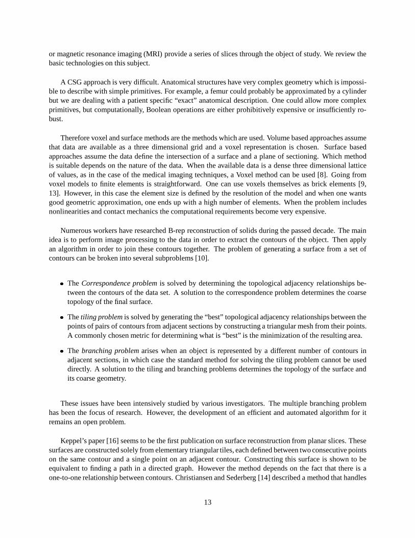
or magnetic resonance imaging (MRI) provide a series of slices through the object of study. We review thebasic technologies on this subject.

A CSG approach is very difficult. Anatomical structures have very complex geometry which is impossi-ble to describe with simple primitives. For example, a femur could probably be approximated by a cylinderbut we are dealing with a patient specific “exact” anatomical description. One could allow more complexprimitives, but computationally, Boolean operations are either prohibitively expensive or insufficiently ro-bust.

Therefore voxel and surface methods are the methods which are used. Volume based approaches assumethat data are available as a three dimensional grid and a voxel representation is chosen. Surface basedapproaches assume the data define the intersection of a surface and a plane of sectioning. Which methodis suitable depends on the nature of the data. When the available data is a dense three dimensional latticeof values, as in the case of the medical imaging techniques, a Voxel method can be used [8]. Going fromvoxel models to finite elements is straightforward. One can use voxels themselves as brick elements [9,13]. However, in this case the element size is defined by the resolution of the model and when one wantsgood geometric approximation, one ends up with a high number of elements. When the problem includesnonlinearities and contact mechanics the computational requirements become very expensive.

Numerous workers have researched B-rep reconstruction of solids during the passed decade. The mainidea is to perform image processing to the data in order to extract the contours of the object. Then applyan algorithm in order to join these contours together. The problem of generating a surface from a set ofcontours can be broken into several subproblems [10].� The Correspondence problem is solved by determining the topological adjacency relationships be-

tween the contours of the data set. A solution to the correspondence problem determines the coarsetopology of the final surface.� The tiling problem is solved by generating the “best” topological adjacency relationships between thepoints of pairs of contours from adjacent sections by constructing a triangular mesh from their points.A commonly chosen metric for determining what is “best” is the minimization of the resulting area.� The branching problem arises when an object is represented by a different number of contours inadjacent sections, in which case the standard method for solving the tiling problem cannot be useddirectly. A solution to the tiling and branching problems determines the topology of the surface andits coarse geometry.

These issues have been intensively studied by various investigators. The multiple branching problemhas been the focus of research. However, the development of an efficient and automated algorithm for itremains an open problem.

Keppel’s paper [16] seems to be the first publication on surface reconstruction from planar slices. Thesesurfaces are constructed solely from elementary triangular tiles, each defined between two consecutive pointson the same contour and a single point on an adjacent contour. Constructing this surface is shown to beequivalent to finding a path in a directed graph. However the method depends on the fact that there is aone-to-one relationship between contours. Christiansen and Sederberg [14] described a method that handles

13

some branching structures but requires user intervention in complex cases. Various researchers proposedmethods based on a concatenation of contours. Boissonat [17] proposed a solution based on a Delaunaytriangulation between each pair of slices. First, the volume of the object is created and then the boundaryis extracted. This method is difficult to implement and does not take into account the topological similarityof the contours. Nevertheless, as a general method, it produces nice results and its code is available on theInternet

�. Note though, that the Delaunay triangulation does not pose any constraints to the quality of the

triangulation.

All these approaches result in a ��� surface. From our experience these surfaces might create prob-lems during the meshing stage. Usually triangulation algorithms are devised for visualization purposes andtherefore they do not pose any constraints on the shape of the triangles. When this kind of triangulationis pipelined to a mesh generator it might lead to failure since the meshing algorithm respects the specifiedboundary. Again researchers have worked on this field to produce smooth surfaces. Based on the Delaunaytriangulation and barycentric implicit � Bernstein-Bezier patches, Bajaj [11] has devised an algorithm for��� surfaces. Algorithms which take a � � piecewise surface and produce ��� piecewise surfaces also exist.Two different approaches include that of Jimenez [19], in which the surface is represented using trigono-metric interpolation, and Meyling [18] who uses B-spline functions in spherical coordinates to representstarlike � � objects. Bajaj [10] explores a technique that goes from the points to the mesh without attemptingany surface reconstruction. The algorithm creates an unstructured 3D triangular (tetrahedral) mesh of thesolid. However, if one wants to perform Boolean operations to the anatomical structure this approach isinadequate.

2.3 A Simple Approach

The problem is how to use CT-scan data in order to describe mathematically the femur and create a com-putational mesh based on this description. We decided to use B-rep methods. First we extract the contoursof the femur and then we pass a surface through these contours. We are using ANSYS 5.2 and PATRANP3/MSC as mesh generators and solvers. From the beginning, voxel methods were excluded since the afore-mentioned packages do not offer any interface to this representation. In the first place we have used a publicdomain triangulation program (nuages), which is based on the algorithm described in [17].

One issue not often mentioned in the literature was the quality of the CT-scan data. As we will see, theprocedure of extracting the boundaries of the object under consideration is still under development, and thecurrent practices induce error to the output data. Usually human intervention is necessary in order to processthe CT-scan, with the aid of imaging software. This procedure produces 300-1000 points per contour. Forthe pelvis approximately 200 slices are used to describe its geometry. This makes a total of 200K pointsto interpolate. It is apparent that any algorithm whose complexity is greater than ��������� gets prohibitivelyslow � � . The most important problem is that this complexity will propagate to all the steps of the analysis;that is, displaying, meshing, and solving.!

Currently at: http://www.inria.fr/prisme/personnel/geiger/nuages.html"Implicit surfaces are algebraic surfaces i.e. given in the form: #%$'&)(+*,(+-/.103254+27682:9<;>=@? . On the other hand parametric

surfaces are given in the following form: &BAC0D&)$FE>(HG�.I(H*JAC0K*,$FEL(:G�.I(M-JAC0D-N$FE>(�G�. .� �A starlike solid is one that has at least one internal point such that the lines connecting this point and all the points on the

surface of the object are internal.�+�For example the worst case complexity for the Delaunay triangulation in the O � is PQ$F; � . and the worst case for incremental

Delaunay triangulation is PQ$F; � . [17]

14

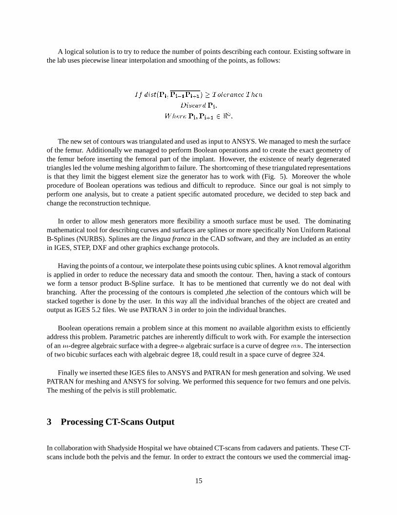
A logical solution is to try to reduce the number of points describing each contour. Existing software inthe lab uses piecewise linear interpolation and smoothing of the points, as follows:

R)S�TVUHWYX �+Z\[H] Z\['^`_/Z7[bac_N�JdfehgNi+j/kNlV�nm�jQehopj/�qDUHW m�l)k T Z7[Hrs otj,kNj1Z [ ]uZ [bac_wvyxJz rThe new set of contours was triangulated and used as input to ANSYS. We managed to mesh the surface

of the femur. Additionally we managed to perform Boolean operations and to create the exact geometry ofthe femur before inserting the femoral part of the implant. However, the existence of nearly degeneratedtriangles led the volume meshing algorithm to failure. The shortcoming of these triangulated representationsis that they limit the biggest element size the generator has to work with (Fig. 5). Moreover the wholeprocedure of Boolean operations was tedious and difficult to reproduce. Since our goal is not simply toperform one analysis, but to create a patient specific automated procedure, we decided to step back andchange the reconstruction technique.

In order to allow mesh generators more flexibility a smooth surface must be used. The dominatingmathematical tool for describing curves and surfaces are splines or more specifically Non Uniform RationalB-Splines (NURBS). Splines are the lingua franca in the CAD software, and they are included as an entityin IGES, STEP, DXF and other graphics exchange protocols.

Having the points of a contour, we interpolate these points using cubic splines. A knot removal algorithmis applied in order to reduce the necessary data and smooth the contour. Then, having a stack of contourswe form a tensor product B-Spline surface. It has to be mentioned that currently we do not deal withbranching. After the processing of the contours is completed ,the selection of the contours which will bestacked together is done by the user. In this way all the individual branches of the object are created andoutput as IGES 5.2 files. We use PATRAN 3 in order to join the individual branches.

Boolean operations remain a problem since at this moment no available algorithm exists to efficientlyaddress this problem. Parametric patches are inherently difficult to work with. For example the intersectionof an { -degree algebraic surface with a degree- � algebraic surface is a curve of degree {K� . The intersectionof two bicubic surfaces each with algebraic degree 18, could result in a space curve of degree 324.

Finally we inserted these IGES files to ANSYS and PATRAN for mesh generation and solving. We usedPATRAN for meshing and ANSYS for solving. We performed this sequence for two femurs and one pelvis.The meshing of the pelvis is still problematic.

3 Processing CT-Scans Output

In collaboration with Shadyside Hospital we have obtained CT-scans from cadavers and patients. These CT-scans include both the pelvis and the femur. In order to extract the contours we used the commercial imag-

15

ModelGenerationFor Trangulated Femur

Figure 5: Surface reconstruction using triangulation and Boolean operations.

16

ing package AVS � � . This package uses modules ( functions) to perform operations and is programmable.The program to do contour extraction was developed by the MRCAS � z group of the Robotics Institute atCarnegie Mellon University.

The thresholding technique is used to separate bone from soft tissue. In the grey scale lighter regionsindicate dense material and the dark regions softer material. Using an upper and a lower value we can createsets of points whose grayscale color corresponds to bone. Then a seed is inserted to the regions of interest todistinguish between different regions of bone ( pelvis and femur in our case). This seed is propagated fromslice to slice in the vertical direction �H| . The next step is to create a closed region and extract the boundaryof this region. Sometimes the bone quality is such that human intervention is necessary in order to completethis task. The output of the file is the one required by the nuages code and is described in the Appendix.

4 Triangulation

Our first approach was to use existing code for surface reconstruction. The intermediate step of linearapproximation of the contours did not work that well. The resulting tessellation had almost degeneratetriangles which led to the failure of the mesh generator. However we consider this approach as an alternativebecause it handles the problem of branching and is fully automated.

Our code allows the user to choose the approximation error and thus determine the number of pointswhich define each (piecewise linear) contour and the step between the slices. This is an implicit way tocontrol the size of the triangles which in turn defines an upper bound to the element size during the meshgeneration.

Furthermore, if one wants to work with a smoother surface there are ways to obtain a � � or a ���triangulation starting from a � � one. Ihm [12] uses algebraic quintic surfaces and Hermite interpolation. Asimilar approach is followed by Menon [22] who uses trunctets to construct the surface, essentially usingalgebraic surfaces. He transforms a B-rep solid to union of truncated tetrahedra which have one facet in theform of an algebraic surface. Fong [21] and Garcıa [20] use barycentric coordinates and B-Spline patches.The basic idea is to average the normals of a set of triangles and fit polynomial surfaces. Algebraic patcheshave the important advantage that they are of lower algebraic degrees so all the computations become easierto perform. The price is reduced flexibility, but in triangulation smoothing this is not a problem.� �

Advanced Visual Systems Inc., 300 Fifth Ave., Aeltham MA 02154� � Medical Robotics and Computer Assisted Surgery� � The coordinate system used has the &L* -plane aligned with the slices.

17

ContourExtraction

with

AVS

Figure 6: Sequence of the thresholding procedure.

18

5 Curve Smoothing

5.1 Mathematical Background

Spline functions (splines) are currently used in diverse domains of numerical analysis ( interpolation, datasmoothing, geometric modeling, numerical solutions of partial differential and integral equations, etc. ).Based on the splines, NURBS have become a standard for describing complex geometries and is imple-mented in every kind of CAD software.

The advantages of splines and NURBS with respect their use in geometric modeling are:� NURBS are genuine generalizations of non rational B-Splines.� They offer a common mathematical form for representing and designing both standard analytic shapes � �and free-form curves and surfaces.� By manipulating the control points as well as the weights NURBS provide the flexibility required todesign complex geometries.� Evaluation is reasonably fast and computationally stable.� B-splines and NURBS have a geometric tool kit ( knot insertion/refinement/removal, degree elevation,splitting, smoothing,etc. ).� B-splines and NURBS are invariant under scaling, rotation, translation and shear as well as paralleland perspective projection.

However they have several drawbacks such as:� Improper application of the weights can result in very bad parameterization, which can destroy sub-sequent surface constructions.� Boolean operations. An example is surface/surface intersection where it is particularly difficult tohandle the “just touch” or “overlap” cases.� Fundamental algorithms as the inverse point mapping are subject to numerical instability.� Displaying algorithms like rendering require � � representation of objects. Thus there is an inherentincompatibility between higher order splines and these algorithms.

So what are a spline function, B-splines and NURBS? A spline is a piecewise polynomial. It consistsof polynomial pieces on subintervals joined together with certain continuity conditions. B-spline theory is away of constructing a group of functions which form a basis for all possible splines up to a degree to a giveninterval and a given knot vector. NURBS is a generalization of B-splines in order to provide more flexibilityand the ability to represent conics exactly.�'

conics, quadrics, surfaces of revolution etc.

19

5.1.1 Splines

Definition. A functionW �+}t� defined on a finite interval ~�lp]5� � , is called a spline function of

T ju�tkNj/jJ�K��� andgNk T j,k%���h���/� , having as ���ng X:W the strictly increasing sequence }���]p������]/�L],r/r�r:]5�B�K�h�+} � ��lt]u} � ^ � ����� ,if the following two conditions are satisfied:

1. On each knot interval ~�} � ]u} � a � ��] W �+}p� is given by a polynomial of degree � at most.} v ~�} � ]5} � a � ��] W �+}t� vy��� ]t������],r/r,r@]5������r (1)

2. The functionW ��}t� and its derivatives up to order ���f� are all continuous on ~�lt]u� � .W �+}t� v � � ^ � ~�lt]u� ��r (2)

Definition. A spline functionW �+}t� is called periodic if in addition to (Eq. 1) - (Eq. 2) it satisfiesW������ �+lV��� W������ �+����]ci`����]/�L],r/r�r@]u�w�f�Lr

Definition. A natural spline function is a spline of odd degree �8� �>i��¡�V�+i�d¢�L� which satisfies theadditional constraints W���� a � � �+lV��� W���� a � � �+��������]t������],�L]/r,r�r@]5i��£��r

We now present a theorem to give an aspect of the geometric properties of the splines. The theorem isvalid for cubic splines but it can be generalized for higher (odd) degree spline functions.

Theorem. LetSp¤C¤

be continuous in ~�lp]5� � and let l¥�¦} ��§ } � § r/r,r § } � ^ � �¦� . IfW

is the natural cubicspline interpolating

Sat the knots ¨t© for ��ª U ª�� then«­¬® ~ W ¤C¤ ��}t�I� � T }yª «­¬® ~ S ¤C¤ �+}t�I� � T }cr

Recall that the curvature of a curve described by the equation ¯�� S ��}t� is the quantity° S ¤C¤ �+}t� ° ~'���²± S ¤ �+}p�u³ � � ^ z5´ � rIt is apparent that the natural spline produces the smoothest possible interpolating function.

The vector space of functions satisfying (1)-(2) will be denoted by µ �Y¶ · and its dimension is ���������[25].

5.1.2 B-Splines

B-splines are a system of spline functions from which all other spline functions can be obtained by form-ing linear combinations. That is, these splines provide bases for certain spline spaces. The B-splines aredistinguished by their elegant theory and their model behavior in numerical calculations.

20

Constant

Quadratic

Linear Cubic

Open Curve

Closed Curve

Tensor Product Surface

B-Splines

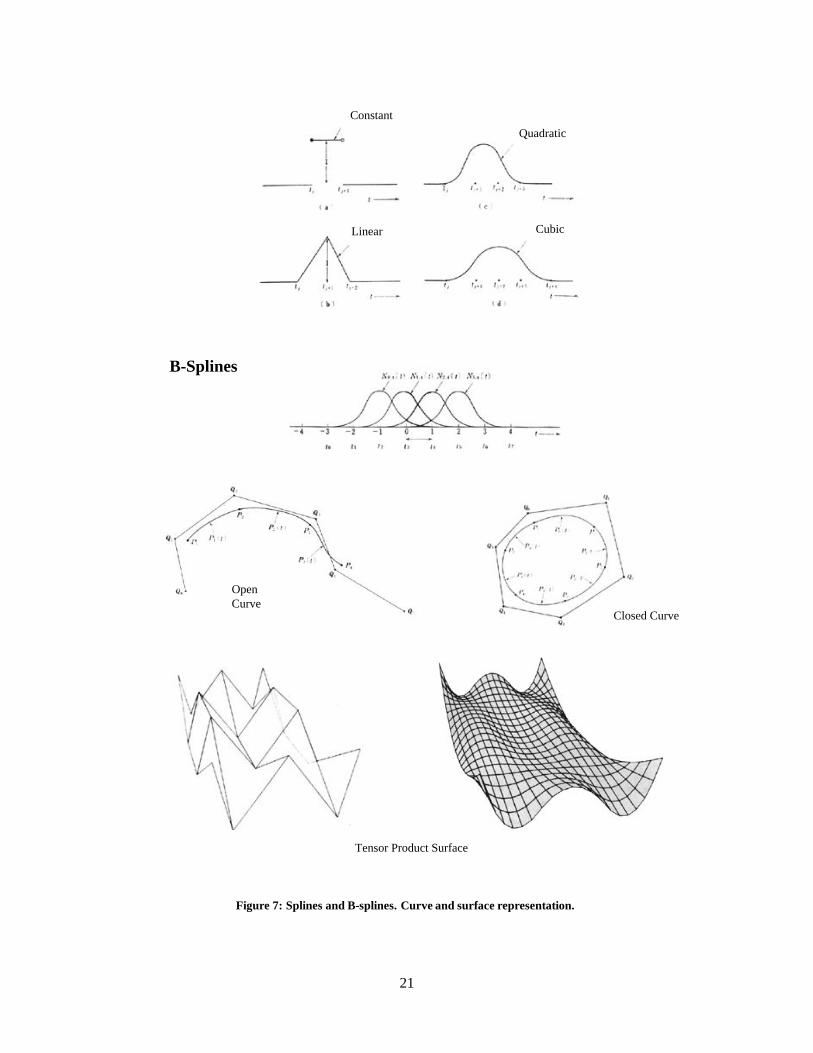
Figure 7: Splines and B-splines. Curve and surface representation.

21

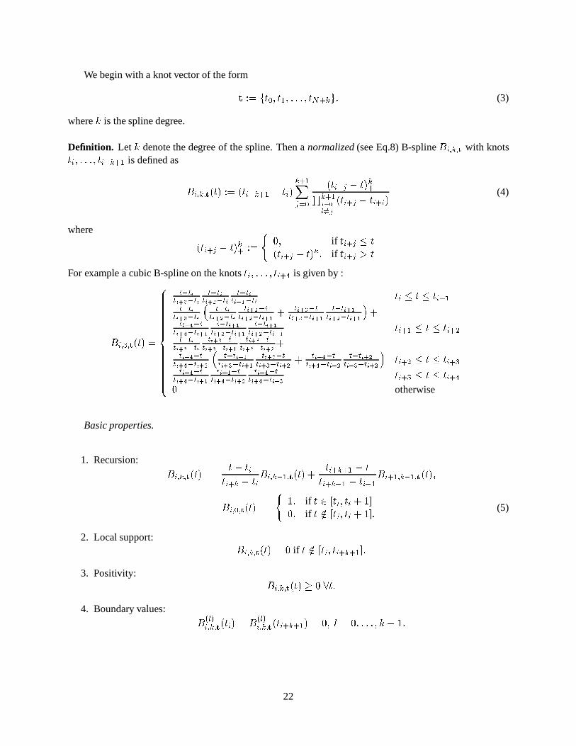
We begin with a knot vector of the form¸w¹ �º± X � ] X � ],r/r/r ] XH» a � ³Vr (3)

where � is the spline degree.

Definition. Let � denote the degree of the spline. Then a normalized (see Eq.8) B-spline ¼½© ¶ �Y¶ · with knotsX ©@],r/r,r�] X ©'a � a � is defined as

¼ © ¶ �Y¶ · � X � ¹ �¾� X ©'a � a � � X © � � a �¿�@À � � X ©�a � � X � �aÁ � a �ÂCà ��FÄÀ�� � X ©'a � � X ©'a � � (4)

where � X ©'a � � X � �a ¹ �ÆÅ ��] ifX ©'a � ª X� X ©'a � � X � � ] ifX ©'a � � X

For example a cubic B-spline on the knotsX ©:]/r/r,r@] X ©'a | is given by :

¼1© ¶ z ¶ · � X ���ÇÈÈÈÈÈÈÈÈÈÈÈÈÈÉ ÈÈÈÈÈÈÈÈÈÈÈÈÈÊ

Ë ^ ËFÌËÍÌ�Î � ^ ËFÌ Ë ^ ËFÌËFÌ�Î � ^ ËFÌ Ë ^ ËFÌËÍÌ�Î � ^ ËFÌ X © ª X ª X ©'a �Ë ^ ËFÌËÍÌ�Î � ^ ËFÌJÏ Ë ^ ËFÌËÍÌ�Î � ^ ËFÌ ËFÌ�Î � ^ ËËFÌ�Î � ^ ËFÌ�Î � � ËÍÌ�Î � ^ ËËFÌ�Î � ^ ËFÌ�Î � Ë ^ ËFÌ�Î �ËFÌ�Î � ^ ËFÌ�Î �/Ð �ËFÌ�Î � ^ ËËÍÌ�Î � ^ ËFÌ�Î � Ë ^ ËFÌ�Î �ËFÌ�Î � ^ ËFÌ�Î � Ë ^ ËFÌ�Î �ËFÌ�Î � ^ ËFÌ�Î � X ©'a � ª X ª X ©'a �Ë ^ ËFÌËÍÌ�Î � ^ ËFÌ ËFÌ�Î � ^ ËËFÌ�Î � ^ ËFÌ�Î � ËÍÌ�Î � ^ ËËFÌ�Î � ^ ËÍÌ�Î � �ËFÌ�Î � ^ ËËÍÌ�Î � ^ ËFÌ�Î � Ï Ë ^ ËFÌ�Î �ËFÌ�Î � ^ ËÍÌ�Î � ËFÌ�Î � ^ ËËÍÌ�Î � ^ ËFÌ�Î � � ËFÌ�Î � ^ ËËFÌ�Î � ^ ËFÌ�Î � Ë ^ ËFÌ�Î �ËFÌ�Î � ^ ËFÌ�Î � Ð X ©'a � ª X ª X ©'a zËFÌ�Î � ^ ËËÍÌ�Î � ^ ËFÌ�Î � ËFÌ�Î � ^ ËËFÌ�Î � ^ ËFÌ�Î � ËFÌ�Î � ^ ËËFÌ�Î � ^ ËFÌ�Î � X ©'a z ª X ª X ©'a |� otherwise

Basic properties.

1. Recursion: ¼Ñ© ¶ ��¶ · � X �Ò� X � X ©X ©'a � � X © ¼1© ¶ � ^ � ¶ · � X �`� X ©'a � a � � XX ©'a � a � � X ©�a � ¼Ñ©'a � ¶ � ^ � ¶ · � X �Y]¼Ñ© ¶ � ¶ · � X �Ò� Å �L] ifX v ~ X ©�] X ©��8�u���] ifX7Óv ~ X ©�] X ©��8�u�Hr (5)

2. Local support: ¼Ñ© ¶ ��¶ · � X �Q��� ifX½Óv ~ X ©:] X ©'a � a � ��r

3. Positivity: ¼Ñ© ¶ �Y¶ · � X �Jd��ÑÔ X r4. Boundary values: ¼ �'���© ¶ �Y¶ · � X ©M����¼ �����© ¶ ��¶ · � X ©�a � a � ������]Õi`����r/r,r/r@]u�w�3�Lr

22

5.1.3 Splines as Linear Combination of B-Splines

Given a knot vector Ö�]��+¨ � �×lt]u¨ � ^ � �Ø��� with � elements we can construct �Ù�¾���¥�Ú�/��� linearlyindependent B-splines of degree k. However, the dimension of µ ��¶ Û is n+k-1 which means that in order toproduce all possible splines in ~�lp]5� � we have to expand the original knot vector. Hence, we need another setof �L� B-splines. So we create an arbitrary new knot vector

¸as follows:X � ª X � ª�Ü,Ü/ÜLª X � ��lp]X ©c��¨ ��Ý U ���`],r/r/r ]5�w�3���f� Ý ������],r/r,r@]5�����Lr (6)�1� X � a � ^ � ª X � a � ª�r/r/rVª X � a � � ^ � r

Thus we can construct n+k-1 B-splines ¼ © ] U �Þ��]/r,r/r@]u���8�K�8� . Let ßØ�Þ�D�8�D��� then every splineW � X � v µ ��¶ Û has a unique representation: W � X �à� » ^ �¿ © À � m © ¼ © ¶ �Y¶ · � X ��] (7)

in which the mu© are called the B-spline coefficients ofW � X � . An important property of B-splines is that:� a � ^ �¿© À � ¼ © ¶ � � X �àáâ��Ô X v �+lp]5����r (8)

B-splines have many other properties like convexity, affinity, rules for integration and differentiation, etc.For more details see [23, 25, 26, 27].

Another important feature of B-spline functions is that one can use a family of discrete norms whichapproximate the usual ãåä -norms well, at least for moderate values of k. Recall that the ãæä -norm of a functionW

is defined by ç W çuè>é �ÆÅ �+ê ° W ° ä � � ´ ä ] for ��ªÒë­ª�ìsup

° W ° ] for ëD��ìand similarly the í ä -norm of a vector î v­x � is defined byç î ç ïÍé �¾Å �+ð © ° l>© ° ä �u� ´ ä ] for �7ªÙë­ª3ì

max © ° l © ° ] for ë���ìIf

W ��ñ�ò·có where ñcò­�Æ�+¼ � ¶ ��¶ · ],r/r,r@]5¼ » ^ � ¶ ��¶ · �:ò the í ä ] ¸ -norm ofW

is defined byç W ç ïÍé �¾Å �+ð © ° mu© ° ä � X ©'a � a � � X ©H� Ó �+�h���/�@�u� ´ ä ] for �wªôëKª�ìmax © ° mu© ° ] for ë¥��ì (9)

which can be written as

ç W ç ï é ¶ · � õõõ�ö � ´ ä· ó õõõï é

, where ö � ´ ä· is a diagonal matrix of dimension ß withdiagonal elements jY© ¶ ©c� Å �@� X ©'a � a � � X ©H� Ó �+�B�8�/�@� � ´ ä ] for �7ªôë­ª�ì�L] for ë���ì (10)�'�

Each B-spline ÷ Ì�ø ù ø ú starts to the û th knot and extends to the $FûNü�ýàüDþ@. th knot.

23

The use of these norms is justified by the following inequality [23] , which denotes the equivalence ofthe í5ä)] ¸ norms and the usual ãåä norm.q ^ �� ç W ç ïFé ¶ · ª ç W ç èLé ª ç W ç ïÍé ¶ · (11)

Hereq � is a constant which depends only on � and for �K�¾ÿ q � �Ú�/��r��Lÿ [23, 25]. These norms will be

essential in the knot removal procedure.

5.1.4 Non Uniform Rational B-splines

When the theory of B-splines was under development most algorithms used a uniform distribution of theknots meaning that they were equally spaced. This caused high oscillations between control points and ingeneral poor results when fitting points which were unevenly spaced. The definition of B-splines given inthe previous section, is general and valid for non-uniform knot vectors.

A further step is to introduce the idea of weights associated with each spline B-spline coefficient.

Definition A NURBS spline is given from the following formula:W � X �à� ð » ^ �© À ��� ©Fmu©M¼Ñ© ¶ � � X �ð » ^ �© À ��� © ¼ © ¶ � � X � r (12)

The knot vector

¸on which the spline is defined is again the same as in (Eq.6). As we can see when all� ©c�Æ� we obtain the B-splines representation. The NURBS form was introduced to deal with the problem

of exact representation of analytic shapes, and to introduce higher flexibility in the user interactive design.It is possible also to have NURBS and B-splines with identical knots in order to represent discontinuities.However, for our purpose B-spline representation with non-repeating knots is adequate. Hence, to avoidunnecessary software complexity from now on we will refer only to non-rational non-uniform B-splines.

5.1.5 Bivariate Splines

The theory of one-variable splines can be extended in different ways to functions of more than one vari-able. The most common are the tensor product splines [23]. Most of the algorithms applied to univariatesplines can be applied also to tensor product splines, but their restriction to rectangular domains is a seriousdisadvantage. As we mentioned before other types of splines ( over triangular domains) are more flexible.However they are far more complex and therefore computationally less attractive.

Definition. Consider the strictly increasing sequencesl�� � �½§ � � § Ü/Ü,Ü § � � ^ � ���N]m1��� � § � �h§ Ü,Ü/Ü § ��� ^ � � T rThe function

W �+}c]u¯)� is called a bivariate (tensor product) spline onq �¦~�lp]5� ���£~�mN] T � , of degree �K�3� in }

and iÕ��� in ¯ , with knots�

and � in the } - and ¯ -direction, if the following conditions are satisfied:

24

B-Spline Basis Functions for Tensor Product Surfaces

Source for all spline figures: Curves and Surfaces in CAGD, Fujio Yamaguchi.

Figure 8: Basis functions for bivariate surfaces.

1. On each sub-rectangleq © ¶ � �â~ � © ] � ©'a � ��Ù~�t�N]��p� a � � , W �+}c]u¯)� is given by a polynomial of degree � in} and i in ¯ .

2. The functionW ��}c]5¯V� and all its partial derivatives up to ���f� and i`�f� , are continuous on

q.� ©�a � W �+}�]5¯V�� } © ¯ � v ��� q ��] U ����],r/r/r ]5���3� Ý ������]/r,r/r:]5{Ú�f�>r

Extending the ideas of vector spaces and basis functions, we can express every spline inq

as a linearcombination of B-splines. If we extend the

�and � vectors as we did for the univariate spline we will obtain

two new knots vectors Ö�]� . Let ß �����3���f� , � ��{¦�fi`�f� then:W �+¨c]��)�Õ� » ^ �¿ �� ^ �¿ � mu© ¶ � ¼1© ¶ �Y¶ Û �+¨t��� � ¶ � ¶ � ���V��] (13)

where the ¼Ñ© ¶ ��¶ Û �+}p� and � � ¶ � ¶ � �+¯V� are the B-splines defined on Ö and knot sequences respectively (Eq. 4).

25

5.1.6 B-Spline Representation of Curves and Surfaces

A parametric B-spline curve f in x�� of degree � defined on the knot vector t where each component is aB-spline function with the same knot vector t, i.e.,� � X � ¹ � � S � ],r/r/r ] S � � òS � � X � � ¿ © m �© ¼Ñ© ¶ ��¶ · � X �

......S � � X � � ¿ © m �© ¼Ñ© ¶ ��¶ · � X �g�k� � X � � ¿ © ó ©H¼1© ¶ �Y¶ · � X �Yr (14)

The coefficients ó © of the spline are vectors x�� . They are called also the control points of the spline. Oneproperty of splines is that they belong to the convex hull of their control points. This is important because itdenotes the non-oscillatory nature of splines.

For the surface we use exactly the same pattern. Let � and i be the order of the splines in the ¨ and �direction and let u and v be two knot vectors. Then the bivariate function to represent the surface is givenby: � �+¨c]��)�c� ¿ © ¿ � ó © ¶ � ¼Ñ© ¶ ��¶ Û �+¨p�@¼ � ¶ � ¶ � ���V����ñ ò�Y¶ Û �+¨p����ñ � ¶ � ���V��r (15)

Where again� �Þ��� � ]/r/r,r:]�� � � , and ó © ¶ � are the control points of the surface. Note that Bezier curves and

surfaces are a special case of B-splines and surfaces.

5.1.7 Discrete B-Splines

The theory of discrete B-splines and the associated algorithms were developed to provide a frameworkfor understanding and implementing subdivision techniques for B-splines. Such technologies are usefulfor rendering and interactive design but they turned out to be also useful for numerical approximation andsmoothing.

Consider a spline written in terms of B-splines on a knot vector � and of degree � :� ¹ �¦��� � ]/r,r/r:]�� » a � �Y]W �����à� » ^ �¿© À � mu©+¼1© ¶ �Y¶ � ������rThere are certain situations where it is useful to increase the degrees of freedom of

Wby adding i additional

knots to the already existing ones. Suppose we let � �ÚßÞ�8i and

¸K¹ � � X � ],r/r,r@] X � a � � be the new knotsequence so that �!

¸. With ¼ � ¶ ��¶ · the B-splines on t,

Wcan also be written as a linear combination of this

26

extended basis with unique coefficientsT � :W � X �à� � ^ �¿� À � T � ¼ � ¶ �Y¶ · � X ��r

The problem is given �`]5ßy]���]���] ¸ , as above computeT � . There are several ways to do that. We can choose� points " � ],r/r,r@]�" � ^ � and solve the interpolation problem,� ^ �¿�@À � T � ¼ � ¶ �Y¶ · �#"V©F��� W �#"V©M��] U ����],�L]/r,r�r@]�� ���Lr

IfX � § ">� § X � a � a � ]H������]/r,r/r:]�� �y� , then this set of linear equations has a unique solution

T � ],r/r,r@] T � ^ �[3]. Lyche et al. in [3] propose a method were

T � can computed as follows:T � � » ^ �¿ � �u© ¶ � mu©:]�gNk%$­�'& ó ]�u© ¶ � ��l>© ¶ � a � ¶ (�¶ · �b����rThe numbers � © ¶ � are called discrete splines and the matrix & is called the insertion matrix of order �w�º�from the knot vector � to knot vector

¸.The numbers l)©@�b��� are defined as follows:

Definition. Suppose �<©'a � � �)�u© . Then l>© ¶ � �¾Å � � © ª*� ©'a �� +-,#.0/21�354768/Moreover for �Dd�� and all

U ]I� ,lL© ¶ � a � �¾� X � a � �9�u©M��:t© ¶ � �b���`�����u©'a � a � � X � a � �;:p©�a � ¶ � ���%�Y]where :t© ¶ � a � � Å ® Ì�ø ù:Î �( Ì�Î>ù�Î � ^ ( Ì � © § � ©�a � a �� +<,#.0/=1�354>68/Based on this definition Lyche et al. devised the Oslo algorithm to create the insertion matrix & given � ,tand � provided that �?

¸. Based on their work we have implemented the Oslo algorithm in C. For further

details about derivation and proofs see [3].

5.2 B-spline Curve Smoothing

5.2.1 Statement of the Problem

The contours extracted with the help of AVS consist, on average, of 400-1000 points. Two problems areassociated with this procedure. The first one occurs when user intervention is necessary to modify theboundary of the bone resulting from the thresholding procedure. As a result, an error is introduced and thegeometry becomes abnormal. The second problem is that the same geometry can be reproduced using less

27

points, even in the case when the noise is minimal. This happens because the module of AVS that creates thecontour points does not recognize topological features, for example linear segments, which can describedwith less points.

Since we deal with planar contours we restrict the following formulation in the 2-D problem. Theextension to any higher dimensions is straightforward. Given a set of ß points Z�©c�¾�+}�©�]u¯/©Í��] U ����],r/r,r@]5ßf�� we have to:

1. Interpolate these points with a parametric curve� � X � such that:� � X � ¹ �Æ�+}�� X ��]5¯`� X �@�� � X ©+����Z\©

It is common practice in computational geometry to haveX v ~���]/�u� .

2. Find @à� X � such that:ç � �A@ ç ªCB

in some suitable norm, where B is a given acceptable error.

Many times the first step is skipped if it is known a priori that the data contain errors or due to the largenumber of sampled points. In order to proceed the form of the function

�must be chosen. One may use

polynomials, splines, trigonometric functions or some other suitable basis. In the case that splines are thechoice these additional parameters must be determined:� The degree � of the spline,� The number and the position of the knots

X © ,� The coefficients ó © , (see Eq. 14)

In this work we are using cubic splines �+�Ò� ÿ>� . We do not need any higher continuity of derivativesthus we follow the common practice of the CAD community. As for the other parameters to be determinedthings are not nearly as simple. In the literature several spline fitting algorithms have been described whichdiffer from each other in the choice of the knots and the approximation criterion. Various methods forknot creation have been proposed: least squares, weighted least squares, minimization of functionals, knotinsertion, and knot removal algorithms [30, 31].

Most fitting algorithms deal with the problem of knot selection either arbitrarily or by solving computa-tionally demanding, non-linear [27, 24] problems. For example one might choose to use a uniform partitionon the ~���],�u� interval depending on the number of points. This method is considered obsolete. Another wayis to use arc length approximation. A suitable one for our case is the chord length parameterization. Westart from � and then each subsequent knot is given by the Euclidean distance between the points. Whenthe distance between the points is too big this can lead to incorrect parameterization. Generally the problemwith fitting algorithms is that there might exist another basis (i.e. another knot sequence) which leads tobetter approximation.

28

Because of the amount of data for each contour we believe that the method proposed by Lyche [1, 2]is a suitable one. First we interpolate the points of the contour using a cubic B-spline. Then we applythe knot removal algorithm given in [1]. The idea is that from the original set of points only a few arenecessary to describe satisfactorily the underlying geometry. Taking into account that even the initial set isan approximation of the object boundary, we start with this initial approximation which is easy to compute,but it might contain excessive points or noise, and we perform data reduction and smoothing.

Using the chord length parameterization we obtain the starting knot sequence. Because the points arevery close to each other essentially this is equivalent to the arc length. Also we are guaranteed that we havea dense enough sequence of knots that the “optimal” solution is included to this knot vector.

5.2.2 Knot Vector Creation and Interpolation

We start with the set of points Z � ],r/r/r ]5Z � ^ � . Because the contour we want to approximate is a closed linewe can extend this set as follows: Z � ¹ �8Z � rThen we can define a knot vector î as: l � ����]l>©n� ç Z7©`�ÙZ7©Í^ � ç è � ] U �¦�>]/r/r,r:]5�ÕrWe normalize î in ~���]/�u� , lL©ED l>©l �In order to produce a B-spline basis that spans all the splines on the knot vector î we have to create a newvector

¸. Since we are dealing with periodic splines the knot vector

¸is given by the following relations

[26](for cubic splines ����ÿ ): ¸ ¹ � � X � ],r/r/r ] X � a �X © � l � �8�+l � ��l>©�a � ^ z ��] U ����]/�>]5��]X ©�a z � l>©�] U ����],r/r/r ]5ßy]X ©'a � a | � l � �¡�+l>©'a � �Ùl � ��] U ����],�L]5��rWe can write

�as: � � X �à� � a �¿© À � $�©M¼Ñ© ¶ · � X ��r

where we have suppressed the subscript denoting the degree of the B-spline. To interpolate the given pointswe form the following � equations:� a �¿ © À � $c©+¼1© ¶ · � X � ����Z � ]I�w����],r/r,r@]5�����Lr (16)

An inconsistency appears to exist between the number of equations and the number of unknowns since wehave � equations and �D��ÿ unknowns. However, because the curve is closed the restrictions in continuity

29

and of the fact that Z � ��Z � lead to: $ � � $ � ]$ � a � � $ � ]$ � a � � $ � rBecause of the locality property of the B-splines the resulting matrix is tridiagonal and can be solved with�����n� operations. Of course we have to perform this operation twice, for the } - and ¯ -direction. We have

used the code described in [32].

5.2.3 Knot Removal

Given � points representing a closed contour we have computed the interpolating spline�. The data neces-

sary to define this spline are its degree � , its knot vector

¸and the coefficients matrix $ © . We denote by µ �Y¶ ·

the set of all splines of degree � on the knot vector

¸. So if

¸ � � X � ]/r,r/r@] X � a � � � then µ �Y¶ · is an �+�D�8��� � �dimensional space of functions given byµ �Y¶ · � W ëtlV��±�¼ � ¶ ��¶ · ],r/r,r@]5¼ � a � ^ � ¶ ��¶ · ³VrNote that if �)F

¸then µ ��¶ � F µ �Y¶ · . As we show before we are interested in the restriction of the elements

of µ �Y¶ · to the interval ~ X � ] X � a � � á ~���],�u� . The knotsX � a � ],r/r,r@] X � a � ^ � are called interior knots, and these

are the only knots we try to remove. In [1, 2] they deal with open curves. We had to slightly modify theiralgorithm for closed curves. For closed curves each time we remove knots we have to modify the extendedset, i.e.

X � ]/r/r,r@] X � ^ � andX � a � a � ],r/r/r ] X � a � � in order to assure that the new curve is � � at the end points.

Suppose a norm

ç Ü ç on µ �Y¶ · has been chosen. We want to compute a subspace µ �Y¶ � of lower dimensionand an element @ of µ �Y¶ � such that

ç � �G@ ç § B . In general, it is not necessary to produce the lowest possibledimension. The aim is to reduce the given vector up to an error within reasonable computational time.

The algorithm we are using involves four main components. We refer to these as Weight, Rank, Remove,and Approximate. In the first step we are computing the weights of the knots. These numbers indicate thesignificance of a knot in specifying the spline shape. The second step is to rank these knots. The third stepis, given a specified number of knots, to remove the least important. In the final step, for the given reducedknot vector we compute a spline @��H��� ¸ Ý � � � on this vector which minimizes the “distance” (since eachspline can be considered as a vector) from the original spline. With � we denote the approximation, in ourcase this is a least squares approximation.

When a vector � and a spline @ is computed we may be able to continue the reduction. If � � ¸it means

that all the knots are important within the specified error. If � contains no interior knots this means that allthe knots were removed. In practice we will have some interior knots. We can try to improve our result byremoving more knots. Here is a schematic algorithm:

1. � � � ¸ Ý @ � � �; (Initialize)�

I might appear that there is an inconsistency between the dimension given in (Sec. 5.1.1) and this one. Because we work witha closed curve of ; points is like having ; ü þ points since the one more point (the end of the curve) is implicitly given. Thus thedimension is $F;JüDþ@.)ü�ýJI�þ�0­;àü�ý .

30

2. for i`����]/�L]u��]/r�r�r1. if � has no interior knots then stop;

2. Compute weights; (Weight)

3. Rank knots; (Rank)

4. Binary Search on k1. Initialize k ; (Number of knots to remove)

2. � � � � Ó �ÙkÑ���ng X:W ; ( Remove)

3. @K����� ¸ Ý � � � ; (Approximate)

4. j/kNkNgNkh� ç � �K@ ç; (Compute Error)

5. if j,kNk�gNk § B increase k ;

6. else decrease k ;

5. if kB��� stop;

6. � � a � � � ;

7. @ � a ��@ ;

The algorithm generates a sequence ��µ �Y¶ �ML � of shrinking subspaces of µ ��¶ · and a sequence of approxima-tions �#@ � � such that: � � a � � � rõõ � �K@ � õõ ª*BIn practice the majority of the knots are removed in the first few iterations. We now present some importantdetails of the algorithm.

Weight. Let � � denote the weight corresponding to knot � �� and µ � ¶ � denote the subspace of spline functionson the knot vector � � � � �)� �� � ��� �� ],r/r/r ]�� �� � ]�� �� a � ],r/r,r � The basic idea is to let � � be an approximationto dist � � ]5µ � ¶ � � in some norm. In this implementation we are using the maximum norm. For simplicity inthe notation we will show the method for ià�¾� so that � � á ¸

and @ � á �. It is understood that the same

procedure is applied for ��in�â�L]5��],r/r�r � . We also suppress subscript � . We compute the weight of knotX � and

we set

� � � ç � �K@ ç ï N ¶ · where@ � OQP>RS-T-U L ø � ç � �A@ ç(17)

Because @ v µ � and� v µ · we extend @ in µ ·

@­� �¿ © ó © ¼ © ¶ � v µ �where {Þ���������Ù� for in��� . Since (See Sec. 5.1.7) µ � �µ · , we have

@�� � a �¿ © Vó ©+¼1© ¶ ·31

where (See [1] and Sec. 5.1.7)

Vó á¾� Vó � ] Vó � ] Vó � �à� ÇÈÉ ÈÊ ó ©:] forU ����],�L]/r,r�r:]H�w�Ù���f�� � ó ©t� � © ó ©Í^ � ] forU �f�����`]/r,r/r@]I�7���ó ©Í^ � ] forU �f�V]/r,r/r@]u�w���

and � ©n� �u©'a � a � � X ��u©'a � a � �W�u© ]X�`©c� X � �9�u©�u©'a � ^ � �K�u©So if ó á¾� ó � ] ó � ] ó �u� , Vó áÆ� Vó � ] Vó � ] Vó �u� and $Òá¾��$ � ]�$ � ]�$Õ�@� (Eq. 16) withó � � � ó � ]/r,r/r@] ó � ^ � ^ � � òó � � � ó � ^ � ^ � ],r/r/r:] ó � ^ � � òó � � � ó � ],r/r,r@] ó � � òVó � � � Vó � ]/r,r/r@] Vó � ^ � ^ � � òVó � � � Vó � ^ � ^ � ],r/r/r:] Vó � � òVó � � � Vó � a � ],r/r,r@] Vó � a � � ò$ � � ��$ � ],r/r/r ]�$ � ^ � ^ � � ò$ � � ��$ � ^ � ^ � ],r/r/r ]�$ � � ò$ � � ��$ � a � ]/r,r/r@]�$ � a � � òThe solution for

Vm U is not unique since we are solving an í © � SpX ¯ problem. We can obtain a solution for (Eq.17) by setting ó � � Vó � �Y$ �ó � � Vó � �Y$ �

For ó � solve OQP>R[Z � õõ $æ�à�K& ó � õõ ï N (18)

whereVó � �'& ó � and

&¦�\]]]]]]]]]^

� � Ü,Ü/Ü � �� � ^ � � � ^ � Ü,Ü/Ü � �� � � ^ � ^ � . . ....

......

.... . . � � ^ � �� � Ü,Ü/Ü � � ^ � � � ^ �� � Ü,Ü/Ü � �

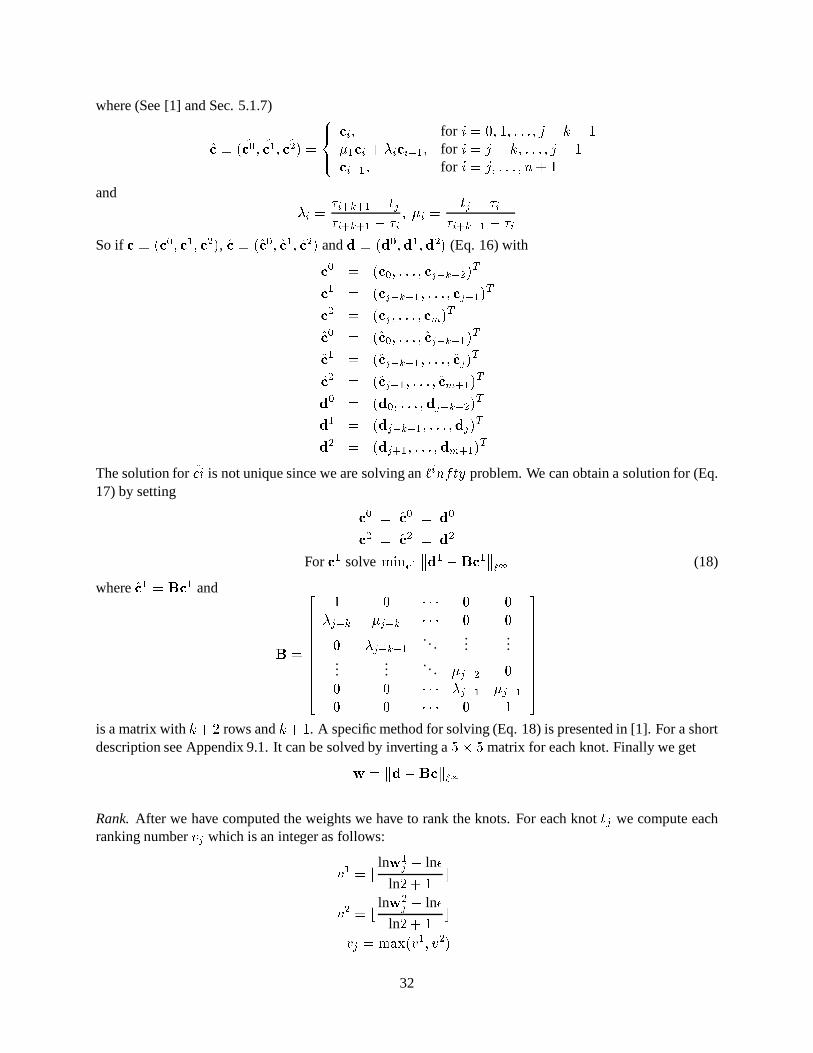
_a`````````bis a matrix with �J�Ò� rows and � �£� . A specific method for solving (Eq. 18) is presented in [1]. For a shortdescription see Appendix 9.1. It can be solved by inverting a cQ�dc matrix for each knot. Finally we gete � ç $y�K& ó ç ï NRank. After we have computed the weights we have to rank the knots. For each knot

X � we compute eachranking number � � which is an integer as follows:

� � �gf lne �� � ln Bln �J���Yh� � �gf lne �� � ln Bln �J���Yh� � �'Ojilkc��� � ]�� � �

32

and then we sort � � in a nondecreasing order.

Remove. If we are to remove k knots from

¸, then we remove all the knots whose rank is strictly less than�2m . Because many knots might have equal ranks it is possible that the number of knots we removed is less

than k . To choose the remaining, say ë knots to be removed, let ¨ � ªÆÜ/Ü,Ünªº¨on be the knots with rankingnumbers equal to � m listed in the order in which the occur in

¸. We remove ��¨ � � ]/r,r/r@]u¨ � é�p � � , whereT ©c�qf ��kà���,�/� U �f��rac>�ë �8� h ���

that is we remove the knots uniformly on subscripts.

Approximate This problem is similar to the one which occurred in the ”weight” step but in more general formsince we are removing more than one knot. However, here we use best approximation in the í � ] ¸ -norm. Wewant to compute @ given

�, � ,

¸and � such that:�

¸@�� ð »© À � ó � ¼Ñ© ¶ �Y¶ � � �¿© À �Xr ©F¼Ñ© ¶ ��¶ ·� ��ð �© À � $ � ¼1© ¶ �Y¶ ·OQP>R S ç � �A@ ç ï �

were the norm is explained in (Sec. 5.1.3, Eq. 9, 10). The coefficients r [ which define @ on µ · are computedwith the discrete splines insertion matrix & which we compute with the Oslo algorithm. So we end up witha usual algebraic least squares problem of the form:

OsPtRZ õõõ�ö � ´ �· ��& ó �K$Õ�Nõõõ ï �It is shown [1] that it is advantageous, with respect the condition number of the normal equations of thisleast squares problem, to solve the following for u ,

OQP>Rv õõõ�ö � ´ �· ��& ö ^ � ´ �� u­�K$Õ�Nõõõ �and then ó � ö ^ � ´ �� u . The condition number of the above equation depends only on � and is small for lowvalues of � [23, 1, 25]. A discrete norm is used because it is simple and fast to work with, and the í � ] ¸ -normbecause it gives rise to linear system of equations, and it approximates ãJ� well. However it does not giveany pointwise information about the error. A solution to this problem is the folowing: when measuring theerror in order to decide how many knots to remove, í2w is used. We used both norms and did not observeany noticeable difference. In any case the user can choose the norm in which error is measured.

6 Surface Skinning

Surface skinning is a process of passing a smooth surface through a set of curves [28]. Usually these curvesrepresent cross-sections of an object so they often mentioned as cross-sectional curves. Using the B-splinesrepresentation, it is possible to “force” a surface to assume almost any curve as an parametric curve be it a

33

Before Approximation: 140 PointsAfter Approximation: 28 Points

Before Approximation: 229 PointsAfter Approximation: 30 Points

Before Approximation: 630 PointsAfter Approximation: 41 Points

Before Approximation: 434 PointsAfter Approximation: 36 Points

Before

After

Curve SmoothingInfinite Norm

Figure 9: Results of the curve smoothing procedure

34

piecewise linear curve, conic section or a high order spline. However, in order to skin across the curves ofvarious types, they all have to be made compatible, i.e. the have to have the same degree and to be definedover the same knot vector. The equation of a tensor product b-spline surface is given by� �+¨c]��)�c� ¿ © ¿ � ó © ¶ � ¼Ñ© ¶ ��¶ Û �+¨p�@¼ � ¶ � ¶ � ���V����ñ ò�Y¶ Û �+¨p����ñ � ¶ � ���V��r (19)

In our problem ¨ corresponds toX-variable of each contour and � represent the x -axis of the CT-scan.

Therefore if we hold � fixed, we recover the contour corresponding to the specific x . Recall that � v ~���]/�<� .The compatibility requirement is now apparent. Each curve has to use the same ¼ �Y¶ Û functions, thus � and Ömust be the same for all curves. We can create a knot vector that is the union of all curves’ knot vectors andthen, by using discrete B-splines, we can compute the coefficients of each curve in the new extended splinespace. However, this procedure is inefficient. If we have 40 curves with 20 knots each, the latter techniquewould create yV�Q� �L�s�?y)� control points. It would essentially cancel the previous knot removal operation,and thus we follow a different approach. We divide the ~���]/�u� into �¥�£� intervals and we take the geometricaverage of the knots that lie within each interval. The result of this process is a set of � knots where � isspecified by the user. So comparing with the aforementioned example this average leads to a approximateskinning of the surface by using only �9�Ky)� control points. In practice ÿ>���)y)� knots where enough toreproduce the curves from the curve approximation.

The next step is to interpolate the curves on this new vector. LetÖ�] ��¨ � ]/r,r/r:]5¨ � ����]/r,r/r:]5¨ � a � �â�L]/r,r/r@]u¨ � a � � �be the union knot vector. The vertical direction � -vector is created in th usual way of chord length parame-terization [28, 27]. For each curve � we compute � points as follows:Z7© � � ¿ � $ � � ¼ � ¶ ��¶ Û ��¨�©F�J] U ���`]/r/r,r@]5�����`rwhere $ � are the coefficients of the � th curve on the µ �Y¶ Û . Then we solve the following linear system [26, 28]for � : Z\© ¶ � ��ñ ò�Y¶ Û �+¨�©+����ñ � ¶ � ��� � ��rThe number of operations to solve this system if ���+�z�W{N� where { is the number of curves. The createdB-spline surface is output in the IGES 5.2 formatted file.

Our implementation provides the user with the ability to choose which curves he/she wants to skin.This represents a crude way of data reduction over the � direction. Moreover one can create multiple filesrepresenting different branches of a complicated structure. However, these surfaces will be disjoint andfurther manipulation must take place to put them together. We used PATRAN’s solid modeling features tocomplete this task.

7 Femur Pre-Processing

We applied the described methodologies on CT-scans from patients and cadavers in order to create geometricmodels for the femur and the acetabulum. For the femur we obtain a representation of the surface by using

35

1200 control points, 40 knots for each curve and 30 curves out of 104. The original data file from the AVSextraction procedure contains 60,000-100,000 points while the final file has around 1000-2000 points.

During the THA operation the surgeon has to cut the femoral head and drill a hole into the femur inorder to insert the femoral part of the implant. Therefore, further processing of the femur surface is neededin order to create the final geometry. Our first approach was to use solid boolean operations between the(triangulated) femur volume and auxiliary volumes representing the volume of the material to be removed.This technique worked but the resulting surfaces were very badly shaped and it was impossible to create amesh. The problem can be simplified by splitting this procedure into two parts. The first is the cutting of thefemoral head and the second is the drilling of the intramedullary canal in order to create the cavity in whichthe implant sits. We believe that it is possible to resolve these problems with of-the-shelf algorithms.

The femoral head removal can be simulated as follows. Using 3 points we can describe mathematicallythe plane of the cutting. Then using a surface/plane intersection algorithm we can create a curve whichrepresents the boundary of the final top surface. It is trivial then, to skin this surface with the remainingset of curves and create the final outer surface. Another approach which currently explore by the MRCASgroup is to rotate the CT-scan data and create the contours in planes parallel to the cutting plane and thenjust discard the upper part of the femur.

The creation of the femoral cavity is more tedious to achieve. Computationally, is very difficult toperform surface/surface Boolean operation since the two surfaces are overlapping (Sec. 5.1). The solutionis to use the plane/surface intersection algorithm we mentioned before and create cross-sectional curves onthe same x -planes as of the CT-scan and then perform boolean operations on the two curves set.

We have written a C program which runs in real time within an ANSYS session in order create the theblended femoral cavity (Fig. 10). We also applied these ideas using PATRAN solid modeling modules andthe results are very satisfactory. Furthermore because the resulting surfaces are the conformal mapping ofa rectangular domain they can be meshed using quadrilateral elements, which is important for the contactmechanics analysis. We also managed to mesh the resulting volumes in ����otgN¨tkN� time.

8 Future Work

There are many issues that have to be addressed in order to complete the patient specific pre-operativeanalysis. The surface reconstruction of the femur still needs considerable user intervention. The algorithmsof surface/plane and curve/curve intersection must be integrated into our program.

Another important issue is the variation of the material properties. Cortical bone can with reasonableaccuracy, be modeled as linearly homogeneous isotropic elastic material. In the contrary trabecular boneis in-homogeneously anisotropic, admits large strains and plastifies. Several ideas have been explored inorder to distinguish between cortical and trabecular bone. One is to represent these two regions as differentvolumes. The other one is to allow material properties vary among and within elements. The latter requiresthe development of an interface between CT-Scan data and the mesh generator. The former requires extrawork for the solid modeling.

36

IntramedullaryCanal

BroachingTool

Insertion

Cross-sectional Boolean addition

FinalCavityShape

NewCross-sectionalCurves

Intramedullary canal preparation for implant insertion.

Figure 10: Preparation of femur intramedullary canal using lower level (area instead of volume) Boolean operations

37

CT-scan Data: 104 Slices, 40000 Points. Approximated Data: 104 Slices, 4000 Points

Skinned Surface: 1800 Control Points.

Femur Modeling: Surface Reconstruction

Figure 11: Femur skinning.

38

Femur Modeling:Branching

Figure 12: Femur branching

39

Femur Modeling:Boolean Operations

FinalSolid Model

Cutting Plane

Femur

Figure 13: Boolean operations on femur in order to produce the final model

40

Femur Modeling: Meshing

Final Volume Mesh: 4649 Elements

Surface Mesh

Figure 14: Computational mesh of the femur.

41

Pelvis Modeling

Smoothing

Skinning

Meshing

Figure 15: Application of the method on pelvis.

42

Meshing of the resulting surface is performed by commercial software as we mentioned before. In thecase of femur, one can take advantage of the cylindrical topology. We are developing a module that usesconformal mapping to create a mesh on each curve plane using quadrilaterals and then stack the elementstogether.

The goal of the research undertaken by our team is to improve post-operative quality of life of the patientvia a pre-operative analysis. We hope that with this work we have make a small step toward this goal.

9 Appendix

9.1 Computing the Weights

In this section we consider the problem OQP>RZç & ó �W$ ç ï N

where $ vyx � , ó v­x � ^ � and the matrix & v­x �}| � � ^ � � has the special form

&¦�\]]]]]]]]]^

� � � Ü/Ü/Ü � �� � � � Ü/Ü/Ü � �� � � . . ....

......

.... . . � � ^ z �� � Ü/Ü/Ü � � ^ � � � ^ �� � Ü/Ü/Ü � � � ^ �

_a`````````bThe solution of this problem can be found [1] by solving a linear system of � equations in � unknowns � �~ u���$where for the matrix

~takes the form

~ �\]]]]]]]]]^

� � Ü/Ü,Ü � � �:�7�/� � ^ �� � ^ � � � ^ � Ü/Ü,Ü � � �:�7�/�:� ^ �� � � ^ � ^ � . . ....

......

......

. . . � � ^ � � �� � Ü/Ü,Ü � � ^ � � � ^ � �7�� � Ü/Ü,Ü � � �

_a`````````bIf u­�¾�+} � ],r/r/r ]5} � ^ � � ò solves

~ u���$ then the solution ó is given by m � ��} � for ������],�L]/r,r�r@]5����� .

9.2 Nuages Input File

Assuming that the CT-scan runs on the x -axis and the image produced on the }t¯ -plane The structure of theinput file for nuages is the following: s integer1�'!

In our case ;B0?�43

v integer2 z floatz±floatx floaty...³v integer2 z floatz±float x float y...³where integer1 denotes number of slices and integer2 denotes number of points to each slice. Differentcontours are included in curly brackets within each slice.

References

[1] T. Lyche and K. Mørken. A data reduction strategy for splines. Research Report no. 107, Instituteof Informatics, University of Oslo, February 1987.

[2] T. Lyche and K. Mørken. Knot Removal for Parametric B-spline Curves and Surfaces. ResearchReport no. 109, Institute of Informatics, University of Oslo, March 1987.

[3] T. Lyche and Richard Riesenfeld. Discrete B-Splines and Subdivision Techniques inComputer-Aided Geometric Design and Computer Graphics. Computer Graphics and ImageProcessing, Vol. 14, 87-111, 1980.

[4] Biegler et al. Effect of Porous Coating and Loading Conditions on total hip femoral stemstability. The Journal of Arthoplasty. Vol. 10 No.6 1995, 839-847.

[5] Christoph M. Hoffman and George Venecek, Jr. Fundamental Techniques for Geometric and SolidModeling. CSD-TR-91-044, Technical Report, Purdue University, Department of Computer Science,1991.

[6] H. J. Samet. Design and Analysis of Spatial Data Structures: Quadtrees, Octrees, and otherHierarchical Methods. Addison-Wesley, Redding, MA, 1989.

[7] G. J. Jense. Voxel-based methods for CAD Computer Graphics Forum, Vol. 13, 238-243, 1992.

[8] W. E. Lorensen and H. E. Cline. Marching cubes: A high resolution 3D surface reconstructionalgorithm. Computer Graphics, Vol. 21(4),163-169, July 1987.

[9] J. H. Keyak et al. Three-Dimensional Finite Element Modeling of the Distal Radius: A newmethod to study fracture. Transactions ,42nd Meeting of The Orthopedic Research Society, Vol. 21,Sec 2, February 1996.

[10] Chandrajit L. Bajaj et al. Surface and 3D Triangular Meshes from Planar Cross Sections. CSD-TR-96-002, Technical Report, Purdue University, Department of Computer Science, 1996.

44

[11] Chandrajit L. Bajaj et al. Automatic Reconstruction of Surfaces and Scalar Fields from 3DScans. CSD-TR-94-0001, Technical Report, Purdue University, Department of Computer Science,1994.

[12] Insung Ihm and Chandrajit L. Bajaj. � � Smoothing of Polyhedra with Implicit Algebraic SurfacePatches. CSD-TR-91-060, Technical Report, Purdue University, Department of Computer Science,1991.

[13] Frey et all. Fully Automatic Mesh Generation for 3-D Domains Based upon Voxel sets. Inter-national Journal for Numerical Methods in Engineering. Vol 37, 2735-2753, 1994.

[14] H.N. Christainsen and T. W. Sederberg. Conversion of complex contour line definition into polyg-onal element mosaics. Computer Graphics, Vol.12, Iss.3, 187-192, 1978.

[15] A. B. Ecoule et all. A triangulation algorithm from arbitrary shaped multiple planar contours.ACM Transactions on Graphics, Vol. 10, Iss. 2, 182-199, 1991.

[16] E. Keppel. Approximating complex surfaces by triangulation of contour lines. IBM Journal ofResearch Developments, Vol. 19, 2-11, 1975

[17] J. D. Boissonat. Shape reconstruction from planar cross sections. Computer Vision, Graphicsand Image Processing, Vol. 44, 1-29, 1988.

[18] R. H. J. Gmelig Meyling and P. R. Pfluger. B-Spline Approximation of a Closed Surface. IMAJournal of Numerical Analysis, Vol. 7, 73-96,1987.

[19] J. C. Jimenez, R. Biscay and E. Aubert Parametric Representation of Anatomical Structures ofthe Human Body by Means of Trigonometric Interpolating Sums. Journal of ComputationalPhysics, Vol. 126, 243-250, 1996.

[20] Miguel Angel Garcıa. Efficient Surface Reconstruction From Scattered Points through Geo-metric Data Fusion. IEEE MFI 1994 Proceedings, Las Vegas, 559-566, Oct. 1994.

[21] Philip Fong and Hans-Peter Seidel. Control Points for Multivariate B-Spline Surfaces over Arbi-trary Triangulations. Computer Graphics Forum, Vol. 10, 309-317, 1991.

[22] Jai P. Menon. Constructive Shell Representations For Free-Form Surfaces and Solids. RC-18450, IBM research Report, IBM T.J.Watson Research Center, October 1992.

[23] C. de Boor. A Practical Guide to Splines. Springer-Verlag, New York 1978.

[24] M. G. Cox. Strategies for knot placement in least squares data fitting by splines. NPL report,DITC 101/87,National Physical Laboratory (UK),1987.

[25] Larry L.Schumaker. Spline Functions: Basic Theory. Wiley and Sons, New York, 1981.

[26] Fujio Yamaguchi. Curves and Surfaces in Computer Aided Geometric Design. Springer-Verlag,Berlin, 1988.

[27] Paul Dierckx. Curve and Surface Fitting with Splines. Clarendon Press, Oxford, 1993.

[28] I. Faux and M. Pratt. Computational Geometry for Design and Manufacture. Ellis Horwood,Chichester, 1979.

45

[29] National Bureau of Standards. IGES,Initial Graphics Exchange Specification, version 5.2 USPRO/IPO-100,American National Standard, Gaithersburg, MD, 1986.

[30] W. Boehm, W. Farin and J. Kahmann. A survey of curve and surface methods in CAGD. ComputerAided Geometric Design, Vol. 1, 1-60, 1984.

[31] Les Piegl. On NURBS:A Survey. IEEE Computer Graphics & Applications, Vol. 1, 55-71,1991.

[32] W. H. Press, S. A. Teukolsky, W. T. Vetterling and B. P. Flannery. Numerical Recipes in C, SecondEdition. Cambridge University Press.

46