Accuracy and Ensemble Methods

April 15, 2023Data Mining: Concepts and

Techniques 2

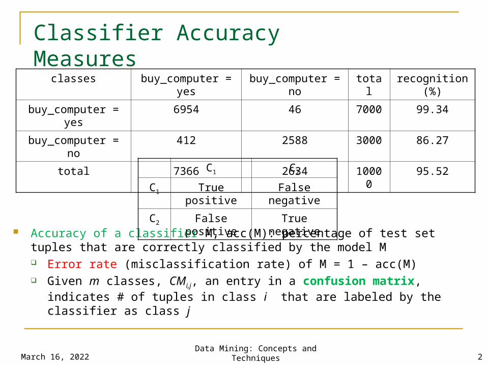
Classifier Accuracy Measures

Accuracy of a classifier M, acc(M): percentage of test set tuples that are correctly classified by the model M Error rate (misclassification rate) of M = 1 – acc(M) Given m classes, CMi,j, an entry in a confusion matrix, indicates # of tuples in

class i that are labeled by the classifier as class j

classes buy_computer = yes

buy_computer = no

total recognition(%)

buy_computer = yes

6954 46 7000 99.34

buy_computer = no

412 2588 3000 86.27

total 7366 2634 10000

95.52C1 C2

C1 True positive False negative

C2 False positive

True negative

Classifier Accuracy Measures Alternative accuracy measures (e.g., for cancer

diagnosis)sensitivity = t-pos/pos /* true positive recognition rate */

specificity = t-neg/neg /* true negative recognition rate */

precision = t-pos/(t-pos + f-pos)

accuracy = sensitivity * pos/(pos + neg) + specificity * neg/(pos + neg)

This model can also be used for cost-benefit analysis Cost associated with misclassification False Positive Vs False Negative

If there is a possibility of tuples belonging to more than one class – probability class distribution may be returned

4

Predictor Error Measures Measure predictor accuracy: measure how far off the predicted value is from the

actual known value

Loss function: measures the error betw. yi and the predicted value yi’

Absolute error: | yi – yi’|

Squared error: (yi – yi’)2

Test error (generalization error): the average loss over the test set Mean absolute error: Mean squared error:

Relative absolute error: Relative squared error:

The mean squared-error exaggerates the presence of outliers Popularly used root mean-square error, similarly root relative squared error

d

yyd

iii

1

|'|

d

yyd

iii

1

2)'(

d

ii

d

iii

yy

yy

1

1

||

|'|

d

ii

d

iii

yy

yy

1

2

1

2

)(

)'(

5

Evaluating the Accuracy Holdout method

Given data is randomly partitioned into two independent sets

Training set (e.g., 2/3) for model construction

Test set (e.g., 1/3) for accuracy estimation

Random sampling: a variation of holdout

Repeat holdout k times, accuracy = avg. of the accuracies obtained

Cross-validation (k-fold, where k = 10 is most popular)

Randomly partition the data into k mutually exclusive subsets, each

approximately equal size

At i-th iteration, use Di as test set and others as training set

Leave-one-out: k folds where k = # of tuples, for small sized data

Stratified cross-validation: folds are stratified so that class dist. in each fold is

approx. the same as that in the initial data

6

Evaluating the Accuracy

Bootstrap Works well with small data sets Samples the given training tuples uniformly with replacement

i.e., each time a tuple is selected, it is equally likely to be selected again and re-added to the training set

.632 boostrap Given a data set of d tuples. The data set is sampled d times, with

replacement, resulting in a training set of d samples. Others form the test set. About 63.2% of the original data will end up in the bootstrap, and the remaining 36.8% will form the test set

Repeating the sampling procedure k times, overall accuracy of the model:

))(368.0)(632.0()( _1

_ settraini

k

isettesti MaccMaccMacc

7

Ensemble Methods: Increasing the Accuracy

Ensemble methods Use a combination of models to increase accuracy Combine a series of k learned models, M1, M2, …, Mk, with the aim of

creating an improved model M* Popular ensemble methods

Bagging: averaging the prediction over a collection of classifiers Boosting: weighted vote with a collection of classifiers Ensemble: combining a set of heterogeneous classifiers

8

Bagging: Boostrap Aggregation Analogy: Diagnosis based on multiple doctors’ majority vote

Training Given a set D of d tuples, at each iteration i, a training set Di of d tuples is sampled

with replacement from D (i.e., boostrap) A classifier model Mi is learned for each training set Di

Classification: classify an unknown sample X Each classifier Mi returns its class prediction The bagged classifier M* counts the votes and assigns the class with the most votes

to X Prediction: can be applied to the prediction of continuous values by taking the average

value of each prediction for a given test tuple Accuracy

Often significant better than a single classifier derived from D For noise data: not considerably worse, more robust Proved to have improved accuracy in prediction

Bagging

10

Boosting Analogy: Consult several doctors, based on a combination of weighted diagnoses—

weight assigned based on the previous diagnosis accuracy

Working

Weights are assigned to each training tuple

A series of k classifiers is iteratively learned

After a classifier Mi is learned, the weights are updated to allow the subsequent

classifier, Mi+1, to pay more attention to the training tuples that were

misclassified by Mi

The final M* combines the votes of each individual classifier, where the weight

of each classifier's vote is a function of its accuracy

The boosting algorithm can be extended for the prediction of continuous values

Comparing with bagging: boosting tends to achieve greater accuracy, but it also risks

overfitting the model to misclassified data

11

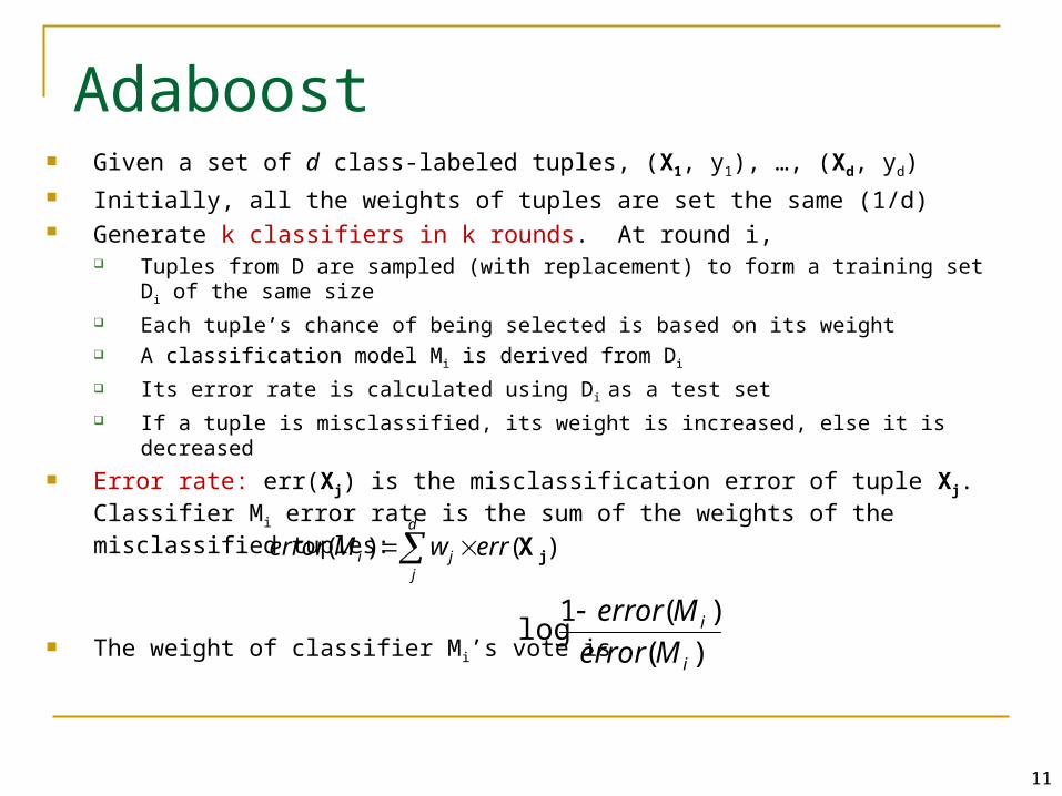
Adaboost Given a set of d class-labeled tuples, (X1, y1), …, (Xd, yd) Initially, all the weights of tuples are set the same (1/d) Generate k classifiers in k rounds. At round i,

Tuples from D are sampled (with replacement) to form a training set D i of the same size

Each tuple’s chance of being selected is based on its weight A classification model Mi is derived from Di

Its error rate is calculated using Di as a test set If a tuple is misclassified, its weight is increased, else it is decreased

Error rate: err(Xj) is the misclassification error of tuple Xj. Classifier Mi error rate is the sum of the weights of the misclassified tuples:

The weight of classifier Mi’s vote is )(

)(1log

i

i

Merror

Merror

d

jji errwMerror )()( jX

Boosting

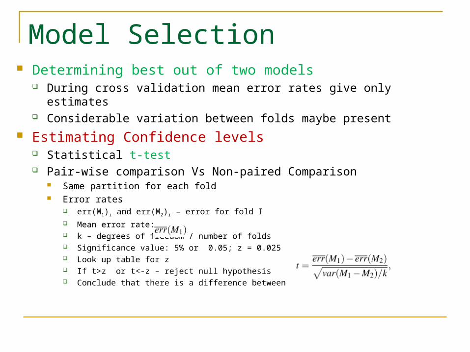
Model Selection Determining best out of two models

During cross validation mean error rates give only estimates Considerable variation between folds maybe present

Estimating Confidence levels Statistical t-test Pair-wise comparison Vs Non-paired Comparison

Same partition for each fold Error rates

err(M1)i and err(M2)i – error for fold I Mean error rate: k – degrees of freedom / number of folds Significance value: 5% or 0.05; z = 0.025 Look up table for z If t>z or t<-z – reject null hypothesis Conclude that there is a difference between the models

14

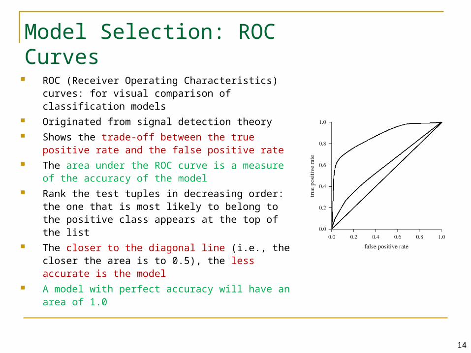
Model Selection: ROC Curves

ROC (Receiver Operating Characteristics) curves: for visual comparison of classification models

Originated from signal detection theory Shows the trade-off between the true positive rate

and the false positive rate The area under the ROC curve is a measure of the

accuracy of the model Rank the test tuples in decreasing order: the one that

is most likely to belong to the positive class appears at the top of the list

The closer to the diagonal line (i.e., the closer the area is to 0.5), the less accurate is the model

A model with perfect accuracy will have an area of 1.0