1

Paper 239-30

Customizing ODS Statistical Graphs Cynthia Zender, SAS Institute Inc., Cary, NC

Catherine Truxillo, SAS Institute Inc., Cary, NC

ABSTRACT Have you heard about ODS Graphics or seen some of the demos? If you are a statistician interested in obtaining easy graphics from statistical procedures, ODS Graphics features provide an automated way of exploring statistical results with a picture. However, if you are a SAS programmer interested in customizing the plots automatically produced by ODS Graphics, you can benefit from an understanding of the graph and style templates that SAS provides for these plots, especially to make changes that persist from one application to the next. Follow the authors on a journey of discovery with ODS Graphics, as they explain how to access and modify graph templates. By the end of the presentation, which includes code samples and demos, you will have a better understanding of the relationship between statistical procedures, graph templates, style templates, and DATA _NULL_ programs. The authors take you through every step of their discovery process.

INTRODUCTION Beginning with SAS®9 a series of new features became available on an experimental basis: ODS Statistical Graphs. These features promise to revolutionize the way that statistical output is presented using SAS software. In order to discuss the highlights of ODS Graphics, we will explore how to modify output using Graph and Style Templates with a DATA _NULL_ program to obtain customized results. Keep in mind that the syntax demonstrated in this paper is unique to SAS 9.1.3 and is still experimental. By the time ODS statistical graphics are production the syntax elements will change. Indeed, the way some procedures work with ODS Graphics will change as well. In the appendix to this paper, the authors have included the full text of some of the SAS 9.1.3 version of the programs; in addition, they have listed a URL from which you can download all 10 demonstration programs. Furthermore, we want to share with you the reasoning and approach behind our paper. Cynthia is the ODS and report person. She's been teaching ODS classes and writing ODS courses since ODS was first introduced. Catherine is the statistics person. She's been teaching and writing SAS/STAT courses since before SAS Version 8. Neither one of us could have done this paper alone. So this paper represents a team collaboration. Cynthia has been getting questions from students about ODS Graphics and how it works for almost a year now. She was motivated to work on a very concrete example to address those questions. But Cynthia is not a statistician. And since every paper needs an organizing principle, something to motivate the paper, Cynthia asked Catherine if there was some example of a statistical graph that she would like to see accomplished using ODS Graphics. Then Catherine told Cynthia about a data set used for some multivariate analysis examples that represented responses to a gambling questionnaire. PROC PRINCOMP was one of the procedures used with the data set for analysis. Rather than see all of the graphs that the procedure produces with ODS Graphics, Catherine wanted to see only the scatterplots for principal components, which are also referred to as scoreplots. Because PROC PRINCOMP produces scoreplots only for the first few principal components, Catherine wanted to know how to plot any combination of the principal component variables, and how to combine two scoreplots into a single display. In the process of discussing how to accomplish these changes, we discussed other changes that would be helpful in the production of customized graphs – such as the use of housekeeping information on the graph, or the addition of a grid or of axis reference lines to the graph. In the process of figuring out how to accomplish this task in SAS 9.1.3, we discovered a lot about the interrelationships between the statistical procedure, the graph template, the style template, and DATA _NULL_. But we have to be very clear. We did not really start with a "problem" to solve. This paper is intended to answer the question "How does ODS Graphics work?" and, as such, presents several different scatterplot examples that enable us to explore ODS Graphics and its interrelationships with other SAS and ODS components. If you are interested in simple ways to use ODS Graphics or easy changes to make, refer to the SUGI paper by Rodriguez (2004). ODS Graphics is very easy to use and most statistical users will seldom need to (or even want to) use some of these techniques. However, for professional SAS programmers who need to create highly customized graphs, or who just want to add to their ODS knowledge, it is essential that they have an understanding of the interaction between graph and style template and how DATA _NULL_ programs can be used with graph templates.

SUGI 30 Tutorials

2

So in the spirit of exploration, we invite you on our journey of discovery.

UNDERSTANDING THE BASICS: OVERVIEW OF ODS STATISTICAL GRAPHICS With ODS Graphics, it is no longer necessary to save data points or results to an output data set, possibly transpose or manipulate the data points, and then display them with a graphical procedure for many of the graphs that analysts commonly use in statistical analysis. For SAS 9.1, a modification to the Output Delivery System (ODS) enables a group of SAS procedures to create statistical graphics as automatically as tables. This feature is referred to as ODS Statistical Graphics (or ODS Graphics). ODS Graphics uses Graph Templates and Graph Style elements to achieve presentation-quality graphical results. Graph template definitions are written in an experimental graph template language, which has been added to the TEMPLATE procedure in SAS 9.1. If a procedure usually has results graphically represented in a certain way (with a scatterplot or a bar chart, for example), then the graphs will automatically be produced if you enable or turn on the ODS Graphics facility (and in some cases, request the plots within the procedure). The list of procedures that currently support ODS Graphics is shown in the following table.

Procedures That Support ODS Graphics SAS/STAT SAS/ETS Other

ANOVA CORRESP GAM GENMOD GLM KDE LIFETEST LOESS LOGISTIC

MI MIXED PHREG PRINCOMP PRINQUAL REG ROBUSTREG

ARIMA AUTOREG ENTROPY EXPAND MODEL SYSLIN TIMESERIES UCM VARMAX X12

CORR (Base SAS) HPF (High-Performance Forecasting)

Since PROC PRINCOMP is used with data from a survey of gambling data, we were interested in whether PROC PRINCOMP supported ODS Graphics. For information about the kinds of graphical output produced for these procedures, consult the SAS®9 documentation for each procedure. For information about the syntax of Graph templates, refer to Chapter 15, "Statistical Graphics Using ODS – Experimental" in the SAS/STAT User's Guide. BASIC ODS GRAPHICS PROGRAM The fundamental method of invoking ODS Graphics is with the combination of ODS GRAPHICS ON/ODS GRAPHICS OFF statements.

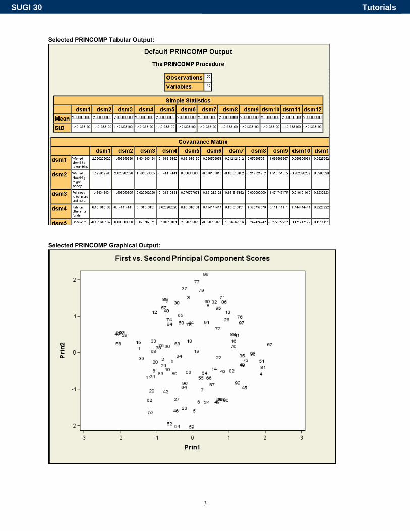
ods html path='.' (url=none) gpath='.' (url=none) file='princomp_default.html' style=statistical; ods graphics on; proc princomp data = work.gamblegrp cov std; title 'Default PRINCOMP Output'; var dsm1-dsm12; run; ods graphics off; ods html close;

If you run this program with the ODS Graphics statements in place, you will find all the tabular output from PROC PRINCOMP followed by all the automatic graphs produced for the analysis. And since ODS Graphics uses Graph style elements, the tables and the graphs will complement each other in terms of colors, fonts, and overall presentation aspects.

SUGI 30 Tutorials

3

Selected PRINCOMP Tabular Output:

Selected PRINCOMP Graphical Output:

SUGI 30 Tutorials

4

METHODOLOGY The steps that we will use to produce and customize our ODS Graphics results will be the same steps that you can follow to investigate any kind of template, not just a graph template:

1. Understand the ODS output object of interest (use ODS TRACE). 2. Select only the ODS output object of interest (use ODS SELECT). 3. Examine the graph template to determine how changes can be made.

a. Modify existing graph template for use with procedure. b. Make custom graph template for use with DATA _NULL_ (optional).

4. Examine the style template of choice to determine any desired changes. 5. Test and refine the templates as needed to produce the desired ODS results.

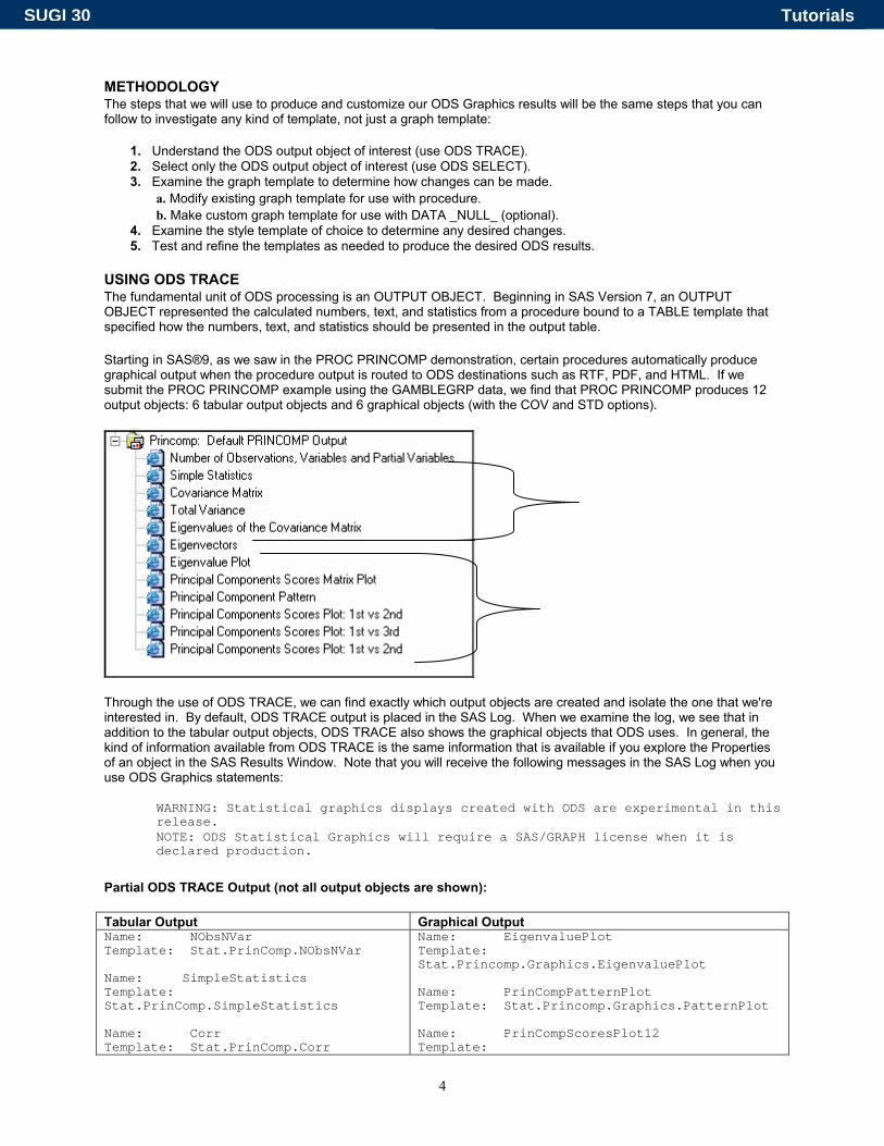
USING ODS TRACE The fundamental unit of ODS processing is an OUTPUT OBJECT. Beginning in SAS Version 7, an OUTPUT OBJECT represented the calculated numbers, text, and statistics from a procedure bound to a TABLE template that specified how the numbers, text, and statistics should be presented in the output table. Starting in SAS®9, as we saw in the PROC PRINCOMP demonstration, certain procedures automatically produce graphical output when the procedure output is routed to ODS destinations such as RTF, PDF, and HTML. If we submit the PROC PRINCOMP example using the GAMBLEGRP data, we find that PROC PRINCOMP produces 12 output objects: 6 tabular output objects and 6 graphical objects (with the COV and STD options).

Through the use of ODS TRACE, we can find exactly which output objects are created and isolate the one that we're interested in. By default, ODS TRACE output is placed in the SAS Log. When we examine the log, we see that in addition to the tabular output objects, ODS TRACE also shows the graphical objects that ODS uses. In general, the kind of information available from ODS TRACE is the same information that is available if you explore the Properties of an object in the SAS Results Window. Note that you will receive the following messages in the SAS Log when you use ODS Graphics statements:

WARNING: Statistical graphics displays created with ODS are experimental in this release. NOTE: ODS Statistical Graphics will require a SAS/GRAPH license when it is declared production.

Partial ODS TRACE Output (not all output objects are shown): Tabular Output Graphical Output Name: NObsNVar Template: Stat.PrinComp.NObsNVar Name: SimpleStatistics Template: Stat.PrinComp.SimpleStatistics Name: Corr Template: Stat.PrinComp.Corr

Name: EigenvaluePlot Template: Stat.Princomp.Graphics.EigenvaluePlot Name: PrinCompPatternPlot Template: Stat.Princomp.Graphics.PatternPlot Name: PrinCompScoresPlot12 Template:

SUGI 30 Tutorials

5

Name: Eigenvalues Template: Stat.PrinComp.Eigenvalues

Stat.Princomp.Graphics.CompScoresPlot Name: PrinCompScoresPlot13 Template: Stat.Princomp.Graphics.CompScoresPlot

Upon examination of the output, we decide that we want to use the PrinCompScoresPlot12 graph object as the "starter" graph.

USING ODS SELECT In a production report or a journal article, we might want tabular output from PROC PRINCOMP included in our ODS output. However, for demonstration purposes, we will limit the output to only the graph of interest. We would use an ODS SELECT statement to limit the output to the single graph object. The previous program is modified to have one of the following ODS SELECT statements: The rule for ODS SELECT is that you can use the short name, the label, the entire label path, or part of the label path or any combination of these component names:

ods select Princomp.PrinCompScoresPlot12; ods select PrinCompScoresPlot12; ods select 'The Princomp Procedure'.'Principal Components Scores Plot: 1st vs 2nd'

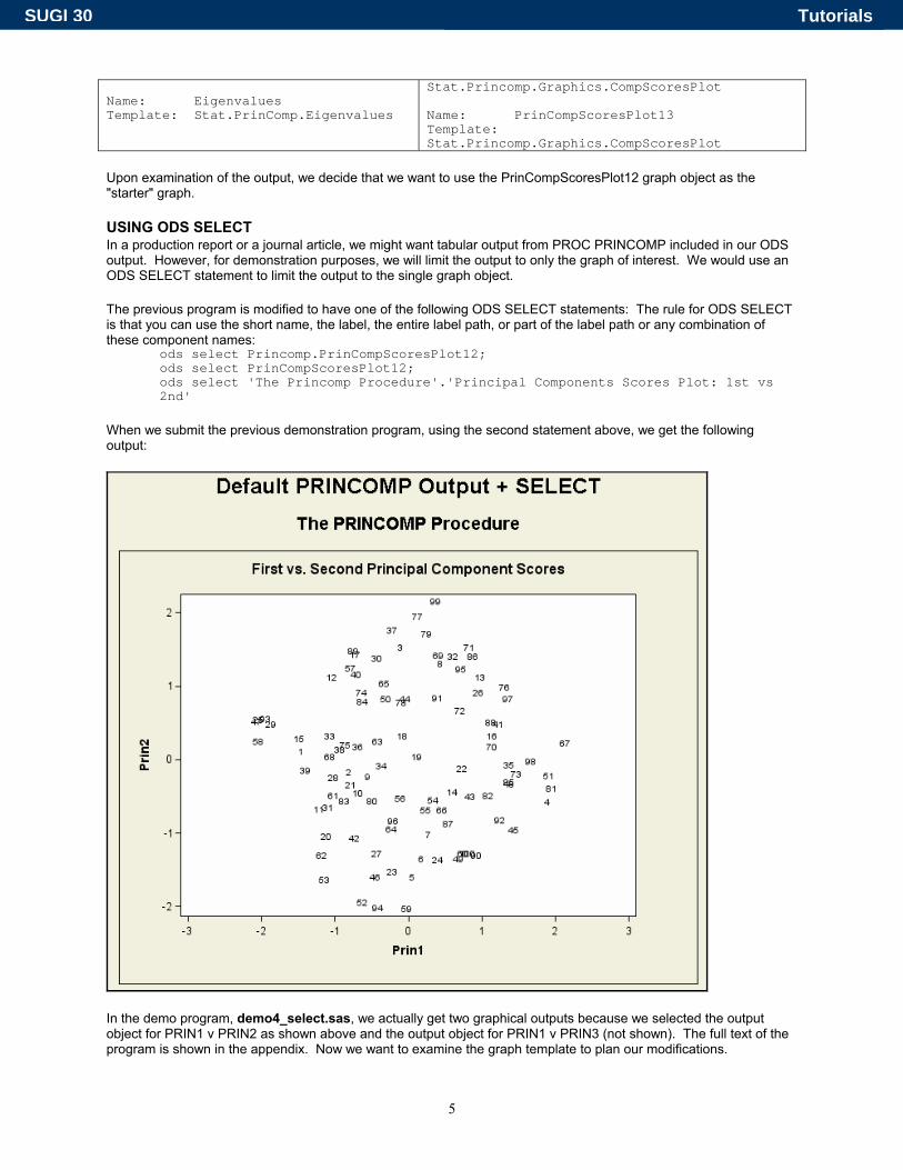
When we submit the previous demonstration program, using the second statement above, we get the following output:

In the demo program, demo4_select.sas, we actually get two graphical outputs because we selected the output object for PRIN1 v PRIN2 as shown above and the output object for PRIN1 v PRIN3 (not shown). The full text of the program is shown in the appendix. Now we want to examine the graph template to plan our modifications.

SUGI 30 Tutorials

6

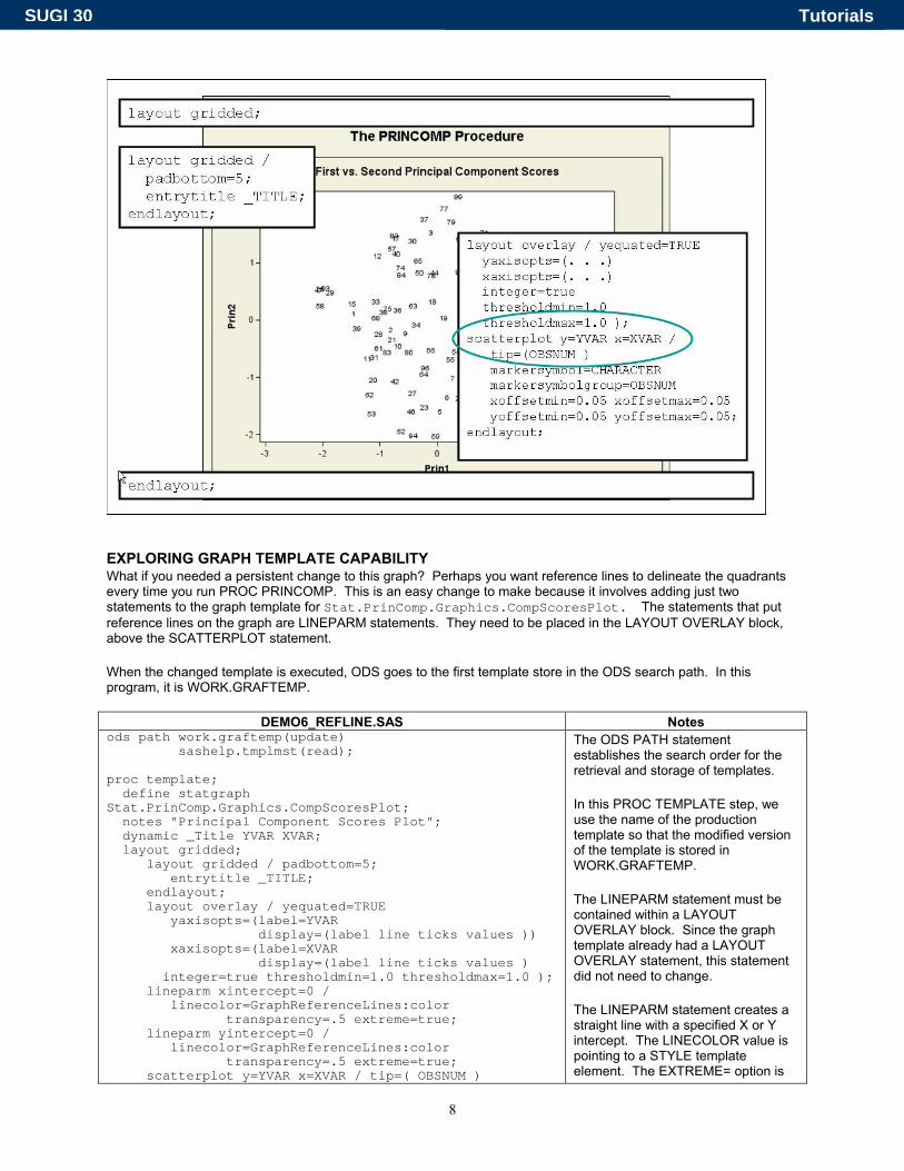
EXAMINE THE GRAPH TEMPLATE Just as you use PROC CONTENTS to see the contents of a SAS data set, you must use either the TEMPLATE Browser or PROC TEMPLATE to view the full text of a SAS template. If you are in an interactive SAS session, you can open the Templates Window by typing odstemplates (or simply odst) on the SAS command line. Or, in the Results Window, place your cursor on the word '”Results" next to the folder and click the right mouse button. In the pop-up menu, select Templates to open the Templates Window. Alternately, you can submit PROC TEMPLATE code to show the template source in the SAS Log Window or write the template source to an external file. The PROC TEMPLATE code is shown below. The first example writes the template source to the SAS Log; the second example writes the template source code to the ASCII text file specified in the FILE= option.

Example 1: Write Template Code to SAS Log Example 2: Write Template Code to File proc template; source Stat.PrinComp.Graphics.CompScoresPlot/

store=sashelp.tmplmst; run;

proc template; source Stat.PrinComp.Graphics.CompScoresPlot/

file='CompScores.sas'; run;

If you use the interactive methods or the first PROC TEMPLATE example, you will see the complete source code that was used to create the compiled template. If you use the second PROC TEMPLATE example and then open the ASCII text file CompScores.sas, you will see the main DEFINE block for the template, but you will not see the opening PROC TEMPLATE statement or the closing RUN statement. If you want to use this code in a PROC TEMPLATE step, you must supply these two required statements. Code in SAS Log or in Template Browser Window proc template; define statgraph Stat.PrinComp.Graphics.CompScoresPlot; notes "Principal Component Scores Plot"; dynamic _Title YVAR XVAR; layout gridded; layout gridded / padbottom=5; entrytitle _TITLE; endlayout; layout overlay / yequated=TRUE yaxisopts=(label=YVAR display=( label line ticks values ) ) xaxisopts=(label=XVAR display=( label line ticks values ) integer=true thresholdmin=1.0 thresholdmax=1.0 ); scatterplot y=YVAR x=XVAR / tip=(OBSNUM ) markersymbol=CHARACTER markersymbolgroup=OBSNUM xoffsetmin=0.05 xoffsetmax=0.05 yoffsetmin=0.05 yoffsetmax=0.05; endlayout; endlayout; end; run; Compare to Code in ASCII file (from FILE= Option of PROC TEMPLATE) (No PROC TEMPLATE statement) define statgraph Stat.PrinComp.Graphics.CompScoresPlot; notes "Principal Component Scores Plot"; dynamic _Title YVAR XVAR; layout gridded; layout gridded / padbottom=5; entrytitle _TITLE; endlayout; layout overlay / yequated=TRUE yaxisopts=(label=YVAR display=( label line ticks values ) ) xaxisopts=(label=XVAR display=( label line ticks values ) integer=true thresholdmin=1.0 thresholdmax=1.0 ); scatterplot y=YVAR x=XVAR / tip=(OBSNUM )

SUGI 30 Tutorials

7

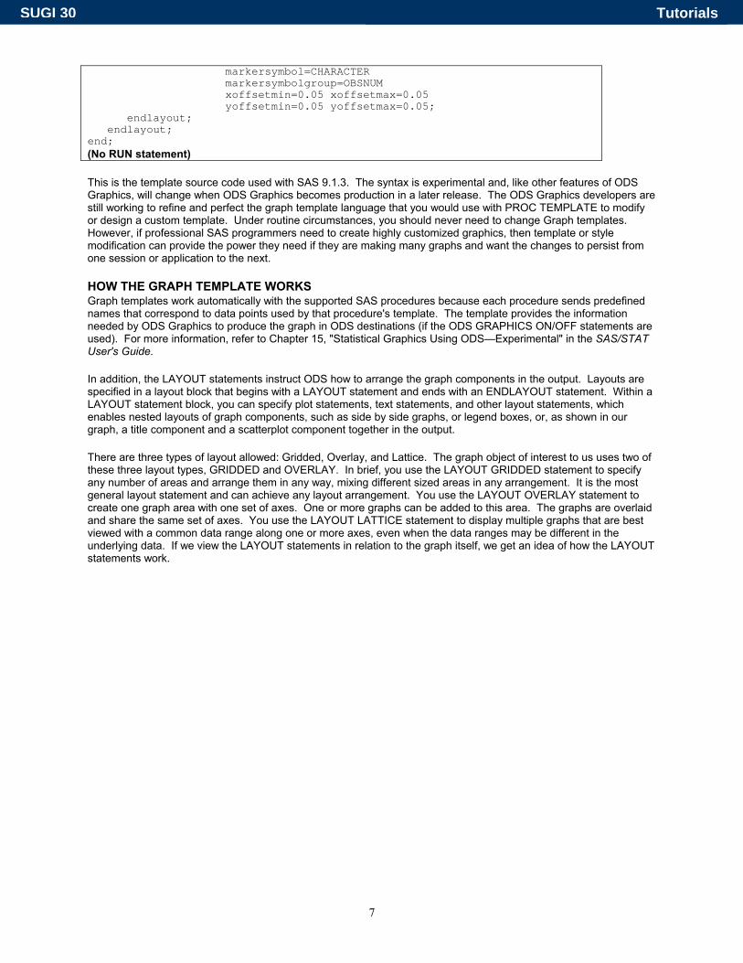
markersymbol=CHARACTER markersymbolgroup=OBSNUM xoffsetmin=0.05 xoffsetmax=0.05 yoffsetmin=0.05 yoffsetmax=0.05; endlayout; endlayout; end; (No RUN statement) This is the template source code used with SAS 9.1.3. The syntax is experimental and, like other features of ODS Graphics, will change when ODS Graphics becomes production in a later release. The ODS Graphics developers are still working to refine and perfect the graph template language that you would use with PROC TEMPLATE to modify or design a custom template. Under routine circumstances, you should never need to change Graph templates. However, if professional SAS programmers need to create highly customized graphics, then template or style modification can provide the power they need if they are making many graphs and want the changes to persist from one session or application to the next.

HOW THE GRAPH TEMPLATE WORKS Graph templates work automatically with the supported SAS procedures because each procedure sends predefined names that correspond to data points used by that procedure's template. The template provides the information needed by ODS Graphics to produce the graph in ODS destinations (if the ODS GRAPHICS ON/OFF statements are used). For more information, refer to Chapter 15, "Statistical Graphics Using ODS—Experimental" in the SAS/STAT User's Guide. In addition, the LAYOUT statements instruct ODS how to arrange the graph components in the output. Layouts are specified in a layout block that begins with a LAYOUT statement and ends with an ENDLAYOUT statement. Within a LAYOUT statement block, you can specify plot statements, text statements, and other layout statements, which enables nested layouts of graph components, such as side by side graphs, or legend boxes, or, as shown in our graph, a title component and a scatterplot component together in the output. There are three types of layout allowed: Gridded, Overlay, and Lattice. The graph object of interest to us uses two of these three layout types, GRIDDED and OVERLAY. In brief, you use the LAYOUT GRIDDED statement to specify any number of areas and arrange them in any way, mixing different sized areas in any arrangement. It is the most general layout statement and can achieve any layout arrangement. You use the LAYOUT OVERLAY statement to create one graph area with one set of axes. One or more graphs can be added to this area. The graphs are overlaid and share the same set of axes. You use the LAYOUT LATTICE statement to display multiple graphs that are best viewed with a common data range along one or more axes, even when the data ranges may be different in the underlying data. If we view the LAYOUT statements in relation to the graph itself, we get an idea of how the LAYOUT statements work.

SUGI 30 Tutorials

8

EXPLORING GRAPH TEMPLATE CAPABILITY What if you needed a persistent change to this graph? Perhaps you want reference lines to delineate the quadrants every time you run PROC PRINCOMP. This is an easy change to make because it involves adding just two statements to the graph template for Stat.PrinComp.Graphics.CompScoresPlot. The statements that put reference lines on the graph are LINEPARM statements. They need to be placed in the LAYOUT OVERLAY block, above the SCATTERPLOT statement. When the changed template is executed, ODS goes to the first template store in the ODS search path. In this program, it is WORK.GRAFTEMP.

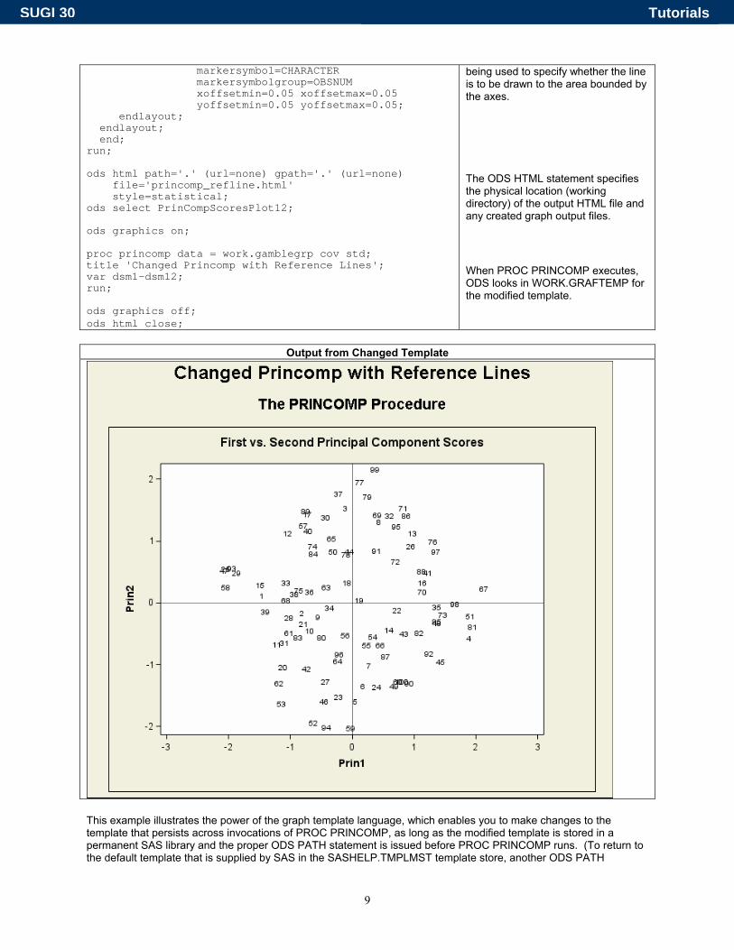
DEMO6_REFLINE.SAS Notes ods path work.graftemp(update) sashelp.tmplmst(read); proc template; define statgraph Stat.PrinComp.Graphics.CompScoresPlot; notes "Principal Component Scores Plot"; dynamic _Title YVAR XVAR; layout gridded; layout gridded / padbottom=5; entrytitle _TITLE; endlayout; layout overlay / yequated=TRUE yaxisopts=(label=YVAR display=(label line ticks values )) xaxisopts=(label=XVAR display=(label line ticks values ) integer=true thresholdmin=1.0 thresholdmax=1.0 ); lineparm xintercept=0 / linecolor=GraphReferenceLines:color transparency=.5 extreme=true; lineparm yintercept=0 / linecolor=GraphReferenceLines:color transparency=.5 extreme=true; scatterplot y=YVAR x=XVAR / tip=( OBSNUM )

The ODS PATH statement establishes the search order for the retrieval and storage of templates. In this PROC TEMPLATE step, we use the name of the production template so that the modified version of the template is stored in WORK.GRAFTEMP. The LINEPARM statement must be contained within a LAYOUT OVERLAY block. Since the graph template already had a LAYOUT OVERLAY statement, this statement did not need to change. The LINEPARM statement creates a straight line with a specified X or Y intercept. The LINECOLOR value is pointing to a STYLE template element. The EXTREME= option is

SUGI 30 Tutorials

9

markersymbol=CHARACTER markersymbolgroup=OBSNUM xoffsetmin=0.05 xoffsetmax=0.05 yoffsetmin=0.05 yoffsetmax=0.05; endlayout; endlayout; end; run; ods html path='.' (url=none) gpath='.' (url=none) file='princomp_refline.html' style=statistical; ods select PrinCompScoresPlot12; ods graphics on; proc princomp data = work.gamblegrp cov std; title 'Changed Princomp with Reference Lines'; var dsm1-dsm12; run; ods graphics off; ods html close;

being used to specify whether the line is to be drawn to the area bounded by the axes. The ODS HTML statement specifies the physical location (working directory) of the output HTML file and any created graph output files. When PROC PRINCOMP executes, ODS looks in WORK.GRAFTEMP for the modified template.

Output from Changed Template

This example illustrates the power of the graph template language, which enables you to make changes to the template that persists across invocations of PROC PRINCOMP, as long as the modified template is stored in a permanent SAS library and the proper ODS PATH statement is issued before PROC PRINCOMP runs. (To return to the default template that is supplied by SAS in the SASHELP.TMPLMST template store, another ODS PATH

SUGI 30 Tutorials

10

statement must be issued to reset the search path so that only SASHELP.TMPLMST is the first template store in the search list.)

ADD IDENTIFYING INFORMATION Other modifications can be performed with the graph template syntax. For example, what if you needed to identify the data set being plotted, or the study name or a date/time stamp? The graph template syntax has several statements that can be used to place housekeeping or administrative information like this onto graphical output. Within graph template syntax, one of the following statements, the ENTRY, ENTRYTITLE, or ENTRYFOOTNOTE statements, could be used to place housekeeping information onto the graph. One company may have the requirement for the study and protocol name to be right justified above the title. Another company may have a requirement for creation date information or data set information to be placed below the main graph area. In order to make use of the appropriate text statements, we must know how we will pass the housekeeping information into the graph template. Through the use of the MVAR statement inside the graph template, we can use SAS macro variable references in the text statements inside our modified template. Information for the macro variables comes from the following %LET statements:

%let kindstudy = Gambling Behavior Study; %let protocol = Protocol: XYZ789; %let create = Created on %sysfunc(today(),mmddyy10.); %let thisdsn = Dataset: work.gamblegrp;

This is the MVAR statement in the template code: mvar kindstudy protocol create thisdsn; Consider how the macro variables are then used inside the modified graph template:

entrytitle kindstudy / halign=right; entrytitle protocol / halign=right; layout gridded / rows=1 border=yes; entry create / foreground=GraphData3:contrastcolor fontfamily=GraphTitleText:font_face fontweight=bold fontsize=12pt; endlayout; entry thisdsn / hAlign=left fontsize=10pt fontweight=bold;

The full text of the program, demo7_housekeeping, can be downloaded from the URL shown in the appendix to this paper. The results from the changed program are shown below:

SUGI 30 Tutorials

11

For demonstration purposes, each of the four macro variables was formatted differently:

1. KINDSTUDY: Right justified using the ENTRYTITLE statement. The font weight is bold because the ENTRYTITLE text is set to bold in the style template.

2. PROTOCOL: Right justified using the ENTRYTITLE statement. As with KINDSTUDY, all the style attributes come from the style template.

3. CREATE: Uses %SYSFUNC to format the current date. This example was run on 1/22/2005. Because the creation date is within a LAYOUT GRIDDED statement, the text is centered by default. Style attributes for the ENTRY statement are specified after the slash (/) in the statement. The style attributes are specified as name/value pairs separated from each other by a space. Each ENTRY or ENTRYTITLE statement ends with one semi-colon.

4. THISDSN: Left justified using an ENTRY statement. Style attributes are specified after the slash (/) in the statement.

Other changes to the graph involve the reference lines. In the original example the reference lines were black, because the line color was set with the following syntax: linecolor=GraphReferenceLines:color In our style template (style=statistical), the value for the color of the GraphReferenceLines element is black. However, in this second example, the LINEPARM statement was modified with the following syntax for the linecolor and linethickness style attributes:

lineparm xintercept=0 / linecolor=GraphData2:contrastcolor linethickness=3px transparency=.5 extreme=true; lineparm yintercept=0 / linecolor=GraphData2:contrastcolor linethickness=StatGraphFitLine:linethickness transparency=.5

SUGI 30 Tutorials

12

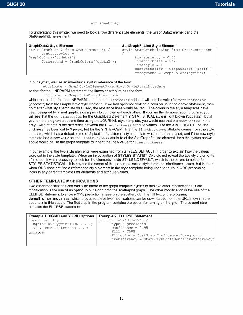
extreme=true; To understand this syntax, we need to look at two different style elements, the GraphData2 element and the StatGraphFitLine element. GraphData2 Style Element StatGraphFitLine Style Element style GraphData2 from GraphComponent / contrastcolor = GraphColors('gcdata2') foreground = GraphColors('gdata2');

style StatGraphFitLine from GraphComponent / transparency = 0.00 linethickness = 2px linestyle = 1 contrastcolor = GraphColors('gcfit') foreground = GraphColors('gfit');

In our syntax, we use an inheritance syntax reference of the form:

attribute = GraphStyleElementName:GraphStyleAttributeName so that for the LINEPARM statement, the linecolor attribute has the form:

linecolor = GraphData2:contrastcolor which means that for the LINEPARM statement the linecolor attribute will use the value for contrastcolor ('gcdata2') from the GraphData2 style element. If we had specified 'red' as a color value in the above statement, then no matter what style template was used, the reference lines would be 'red'. The colors in the style templates have been designed by visual graphics designers to complement each other. If you run the demonstration program, you will see that the contrastcolor for the GraphData2 element in STATISTICAL style is light brown ('gcdata2'), but if you run the program a second time using the JOURNAL style template, you would see that the contrastcolor is gray. Also of note is the difference between the linethickness attribute values. For the XINTERCEPT line, the thickness has been set to 3 pixels, but for the YINTERCEPT line, the linethickness attribute comes from the style template, which has a default value of 2 pixels. If a different style template was created and used, and if the new style template had a new value for the linethickness attribute of the StatGraphFitLine element, then the syntax shown above would cause the graph template to inherit that new value for linethickness. In our example, the two style elements were examined from STYLES.DEFAULT in order to explain how the values were set in the style template. When an investigation of STYLES.STATISTICAL did not reveal the two style elements of interest, it was necessary to look for the elements inside STYLES.DEFAULT, which is the parent template for STYLES.STATISTICAL. It is beyond the scope of this paper to discuss style template inheritance issues, but in short, when ODS does not find a referenced style element in the style template being used for output, ODS processing looks in any parent templates for elements and attribute values.

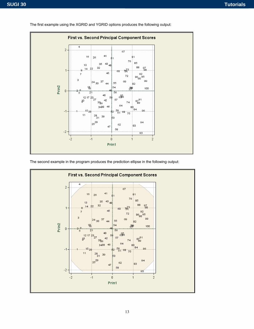
OTHER TEMPLATE MODIFICATIONS Two other modifications can easily be made to the graph template syntax to achieve other modifications. One modification is the use of an option to put a grid onto the scatterplot graph. The other modification is the use of the ELLIPSE statement to show a 95% prediction ellipse on the scatterplot. The full text of the program, demo8_other_mods.sas, which produced these two modifications can be downloaded from the URL shown in the appendix to this paper. The first step in the program contains the option for turning on the grid. The second step contains the ELLIPSE statement: Example 1: XGRID and YGRID Options Example 2: ELLIPSE Statement layout overlay / xgrid=TRUE ygrid=TRUE . . .; <. . more statements . . > endlayout;

ellipse y=YVAR x=XVAR / type = predicted confidence = 0.95 fill = TRUE fillcolor = StatGraphConfidence:foreground transparency = StatGraphConfidence:transparency;

SUGI 30 Tutorials

13

The first example using the XGRID and YGRID options produces the following output:

The second example in the program produces the prediction ellipse in the following output:

SUGI 30 Tutorials

14

The demonstration program used for this output also creates a custom style template called PrinStyle that changes some of the style attributes for two style elements, as shown in the code below: Modified PrinStyle Template proc template; define style styles.PrinStyle; parent = Styles.statistical; style GraphLabelText from GraphComponent / font = GraphFonts('GraphLabelFont') foreground = GraphColors('gcdata3'); style GraphReferenceLines from GraphReferenceLines / foreground = GraphColors('gcdata3') linestyle = 3 linethickness = 2px; style StatGraphConfidence from StatGraphConfidence / transparency = 0.750 linethickness = 1px linestyle = 34 contrastcolor = GraphColors('gcconfidence') foreground = GraphColors('gconfidence'); end; run; Note how the transparency attribute for the ELLIPSE statement inherits this new value of 0.750 as the transparency value rather than the value of 0.50 from the STYLES.DEFAULT template. In the above instance, STYLES.STATISTICAL is the immediate parent template for the new style; however, if a style element is not found in the most immediate parent template, then ODS resolves inheritance by going to the "grandparent" template, which in this instance is the STYLES.DEFAULT template.

EXAMINE THE STYLE TEMPLATE AND DOCUMENTATION The same PROC TEMPLATE code that we saw before can be used to reveal the full contents of both templates involved in the creation of STYLES.PRINSTYLE. In order to construct the PRINSTYLE template, we had to consult the ODS Graphics documentation to determine which style elements were used for the various parts of the graph output. Although any SAS-supplied or user-defined style may be used to create ODS Graphics output (as shown in the above example), four style templates have been specifically designed for use with ODS statistical graphics: DEFAULT, JOURNAL, ANALYSIS, and STATISTICAL. The documentation is very thorough in outlining the graph style elements. For more information about the elements and attributes used inside the style template, consult the Web site http://support.sas.com/rnd/base/topics/statgraph/v91StatGraphStyles.htm, which explains the SAS 9.1 style elements. For example, the following screen shot from the documentation illustrates which style elements affect graphical text style elements:

SUGI 30 Tutorials

15

By investigating the documentation, we discovered that the GraphLabelText element was in control of the text labels for PRIN1 and PRIN2. We modified our style template to use the same color for the GraphLabelText foreground attribute and the GraphReferenceLines foreground attribute.

USING DATA _NULL_ By default, when PROC PRINCOMP produces scatterplots with ODS Graphics, it produces graphs of PRIN1 v PRIN2 and PRIN1 v PRIN3. A simple ODS SELECT statement (as seen in the demo programs) is all that is needed to produce these two scatterplots by themselves, without the other PRINCOMP graphs. However, Catherine wanted to see a comparison of PRIN1 v PRIN2 and PRIN2 v PRIN3. When PROC PRINCOMP creates these two default graph objects, it sends the appropriate X and Y variables needed by the graph template for each scatterplot. In order to see different X and Y variables (like PRIN2 v PRIN3), we need to use a DATA _NULL_ program to instruct the graph template as to which variables from our data set correspond to the X and Y variables needed by the graph template. One of the most powerful features of ODS Graphics is the ability to invoke a graph template using a DATA _NULL_ program. However, before we can create a custom graph template to be used with a DATA _NULL_ step, we need to have the data points to pass to the template. Remember that under most circumstances, you would not need to use a DATA step program to create ODS Statistical Graphs. Most statistical graphs can be produced without saving data points, but the fact that we can save our data points and use them with a DATA _NULL_ program illustrates how ODS Graphics can accommodate everything from simple changes to very stringent and specific graph requirements. Once we create an output data set from PROC PRINCOMP (using the OUT= option), we can pass our data set variables into the custom graph template. The DATA _NULL_ step becomes the communication link between the graph template and the data that we want to see on our version of the scatterplot.

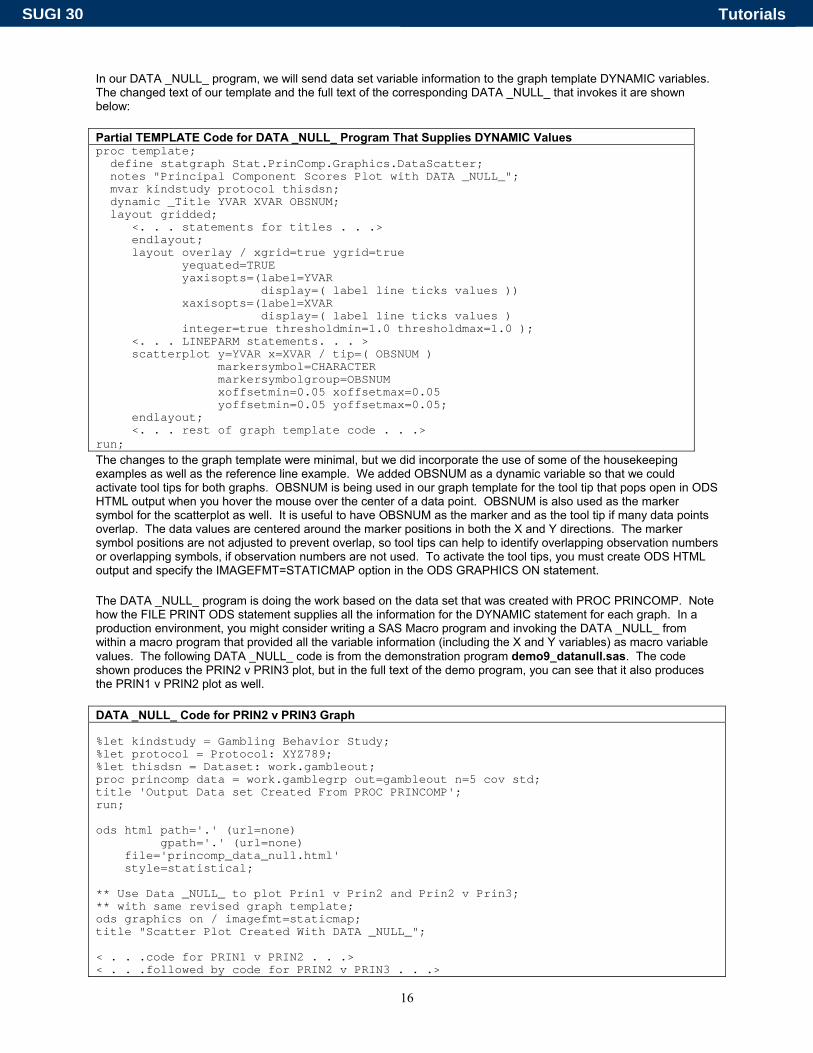
USING DYNAMIC VARIABLES WITH DATA _NULL_ For a more complete description of how graph templates work, consult the SAS/STAT documentation for the supported procedures and see the chapter “Statistical Graphics Using ODS—Experimental” in the SAS/STAT 9.1 User's Guide. The reference section at the end of this paper points you to several very thorough explanations of graph templates written by Jeff Cartier. Since the syntax may change when the ODS Statistical Graphics feature becomes production, we are not going to focus on a statement-by-statement explanation of the syntax. However, we will show you enough to get you started with your own experimentation efforts. Keep in mind that the approach presented in this section should be considered highly experimental. Please do not use these methods for production work, but rather to explore the ways that you can modify graph templates. Consider the DYNAMIC statement in the original template source code: dynamic _Title YVAR XVAR;

SUGI 30 Tutorials

16

In our DATA _NULL_ program, we will send data set variable information to the graph template DYNAMIC variables. The changed text of our template and the full text of the corresponding DATA _NULL_ that invokes it are shown below: Partial TEMPLATE Code for DATA _NULL_ Program That Supplies DYNAMIC Values proc template; define statgraph Stat.PrinComp.Graphics.DataScatter; notes "Principal Component Scores Plot with DATA _NULL_"; mvar kindstudy protocol thisdsn; dynamic _Title YVAR XVAR OBSNUM; layout gridded; <. . . statements for titles . . .> endlayout; layout overlay / xgrid=true ygrid=true yequated=TRUE yaxisopts=(label=YVAR display=( label line ticks values )) xaxisopts=(label=XVAR display=( label line ticks values ) integer=true thresholdmin=1.0 thresholdmax=1.0 ); <. . . LINEPARM statements. . . > scatterplot y=YVAR x=XVAR / tip=( OBSNUM ) markersymbol=CHARACTER markersymbolgroup=OBSNUM xoffsetmin=0.05 xoffsetmax=0.05 yoffsetmin=0.05 yoffsetmax=0.05; endlayout; <. . . rest of graph template code . . .> run; The changes to the graph template were minimal, but we did incorporate the use of some of the housekeeping examples as well as the reference line example. We added OBSNUM as a dynamic variable so that we could activate tool tips for both graphs. OBSNUM is being used in our graph template for the tool tip that pops open in ODS HTML output when you hover the mouse over the center of a data point. OBSNUM is also used as the marker symbol for the scatterplot as well. It is useful to have OBSNUM as the marker and as the tool tip if many data points overlap. The data values are centered around the marker positions in both the X and Y directions. The marker symbol positions are not adjusted to prevent overlap, so tool tips can help to identify overlapping observation numbers or overlapping symbols, if observation numbers are not used. To activate the tool tips, you must create ODS HTML output and specify the IMAGEFMT=STATICMAP option in the ODS GRAPHICS ON statement. The DATA _NULL_ program is doing the work based on the data set that was created with PROC PRINCOMP. Note how the FILE PRINT ODS statement supplies all the information for the DYNAMIC statement for each graph. In a production environment, you might consider writing a SAS Macro program and invoking the DATA _NULL_ from within a macro program that provided all the variable information (including the X and Y variables) as macro variable values. The following DATA _NULL_ code is from the demonstration program demo9_datanull.sas. The code shown produces the PRIN2 v PRIN3 plot, but in the full text of the demo program, you can see that it also produces the PRIN1 v PRIN2 plot as well. DATA _NULL_ Code for PRIN2 v PRIN3 Graph %let kindstudy = Gambling Behavior Study; %let protocol = Protocol: XYZ789; %let thisdsn = Dataset: work.gambleout; proc princomp data = work.gamblegrp out=gambleout n=5 cov std; title 'Output Data set Created From PROC PRINCOMP'; run; ods html path='.' (url=none) gpath='.' (url=none) file='princomp_data_null.html' style=statistical; ** Use Data _NULL_ to plot Prin1 v Prin2 and Prin2 v Prin3; ** with same revised graph template; ods graphics on / imagefmt=staticmap; title "Scatter Plot Created With DATA _NULL_"; < . . .code for PRIN1 v PRIN2 . . .> < . . .followed by code for PRIN2 v PRIN3 . . .>

SUGI 30 Tutorials

17

data _null_; set gambleout; OBSNUM = _N_; file print ods=(template="Stat.PrinComp.Graphics.DataScatter" dynamic=(_Title="Second v Third Principal Component Scores" XVAR="prin2" YVAR="prin3" OBSNUM="OBSNUM") ); put _ods_; run; ods graphics off; ods html close; We gave our modified graph template a unique name, Stat.PrinComp.Graphics.DataScatter, to ensure that the graph template would not accidentally be used if PROC PRINCOMP were invoked using other data. In a production environment, if you were designing highly customized graph templates, you might want to invoke the graph using a DATA _NULL_ program using a unique graph template name that reflected the intended purpose of the graph. As you can see in the above code, the TEMPLATE= option of the FILE PRINT ODS statement enables you to point to a graph template in the same fashion that you use the statement to point to a TABLE template. The output for PRIN2 v PRIN3 is shown below:

CUSTOM GRAPH PLACEMENT Our last modification to the output involves a demonstration of the ability to achieve custom placement of graphics output. What would be helpful for our analysis of the gambling data would be to show the PRIN1 v PRIN2 and PRIN2 v PRIN3 graphs side by side rather than one on top of the other in the output (as shown previously). To achieve this custom graph placement, we need to define all the layout areas on the output area. In this last example, we will look at the output first and then investigate the code.

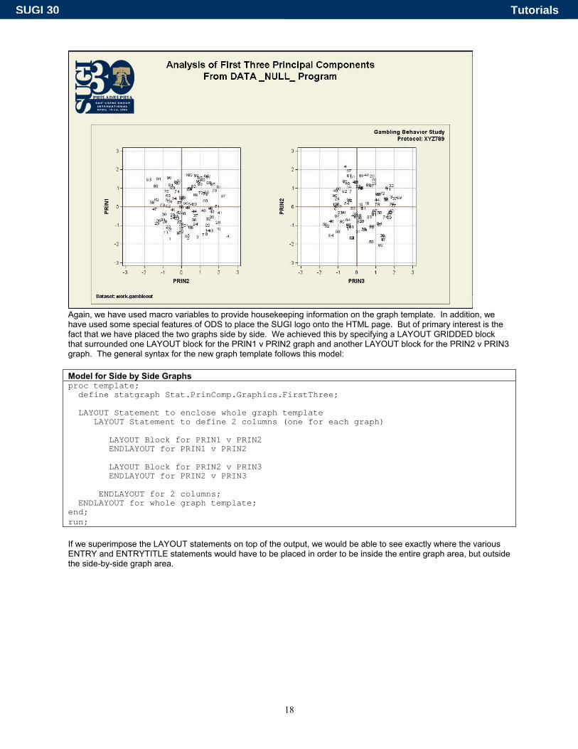
SUGI 30 Tutorials

18

Again, we have used macro variables to provide housekeeping information on the graph template. In addition, we have used some special features of ODS to place the SUGI logo onto the HTML page. But of primary interest is the fact that we have placed the two graphs side by side. We achieved this by specifying a LAYOUT GRIDDED block that surrounded one LAYOUT block for the PRIN1 v PRIN2 graph and another LAYOUT block for the PRIN2 v PRIN3 graph. The general syntax for the new graph template follows this model: Model for Side by Side Graphs proc template; define statgraph Stat.PrinComp.Graphics.FirstThree; LAYOUT Statement to enclose whole graph template LAYOUT Statement to define 2 columns (one for each graph) LAYOUT Block for PRIN1 v PRIN2 ENDLAYOUT for PRIN1 v PRIN2 LAYOUT Block for PRIN2 v PRIN3 ENDLAYOUT for PRIN2 v PRIN3 ENDLAYOUT for 2 columns; ENDLAYOUT for whole graph template; end; run; If we superimpose the LAYOUT statements on top of the output, we would be able to see exactly where the various ENTRY and ENTRYTITLE statements would have to be placed in order to be inside the entire graph area, but outside the side-by-side graph area.

SUGI 30 Tutorials

19

This conceptual look at the graph output and the model syntax together indicates that the housekeeping text statements (for macro variables KINDSTUDY, PROTOCOL, and THISDSN) are interspersed between the various LAYOUT statements. The full text of the program, demo10_datanull_sidebyside.sas, can be downloaded from the Web site http://support.sas.com/rnd/papers/index.html. If you compare the output for PRIN2 v PRIN3 in the above output with the output from the previous program, you will note that the default output graph for PRIN2 v PRIN3 was rectangular in shape (without the COV and STD options). In our program, we used the explicit TICKS= option for each graph's X and Y axis: ticks = (-3 -2 -1 0 1 2 3) This ensures that both graphs are the same shape and have the same tick mark values. In addition, if you examine our graph template, you will see that we hard-coded the X and Y values for each graph so that it was clear which graph layout block produced PRIN1 v PRIN2 analysis and which graph layout block produced the PRIN2 v PRIN3 graph. Partial Layout Block for PRIN1 v PRIN2 Partial Layout Block for PRIN2 v PRIN3 layout overlay / padleft=5 xgrid=TRUE ygrid=TRUE yequated=TRUE yaxisopts=(label=PRIN1 ticks = (-3 -2 -1 0 1 2 3) display=( label line ticks values )) xaxisopts=(label=PRIN2 ticks = (-3 -2 -1 0 1 2 3) display=( label line ticks values ) integer=true thresholdmin=1.0 thresholdmax=1.0 ); <. . . LINEPARM statements . . .> scatterplot y=PRIN1 x=PRIN2/ tip=( TIP_L ) markersymbol=CHARACTER markersymbolgroup=OBSNUM_L <. rest of scatterplot statements .>; endlayout;

layout overlay / padleft=5 xgrid=TRUE ygrid=TRUE yequated=TRUE yaxisopts=(label=PRIN2 ticks = (-3 -2 -1 0 1 2 3) display=( label line ticks values )) xaxisopts=(label=PRIN3 ticks = (-3 -2 -1 0 1 2 3) display=( label line ticks values ) integer=true thresholdmin=1.0 thresholdmax=1.0 ); <. . . LINEPARM statements . . .> scatterplot y=PRIN2 x=PRIN3/ tip=( TIP_R ) markersymbol=CHARACTER markersymbolgroup=OBSNUM_R <. rest of scatterplot statements .>; endlayout;

SUGI 30 Tutorials

20

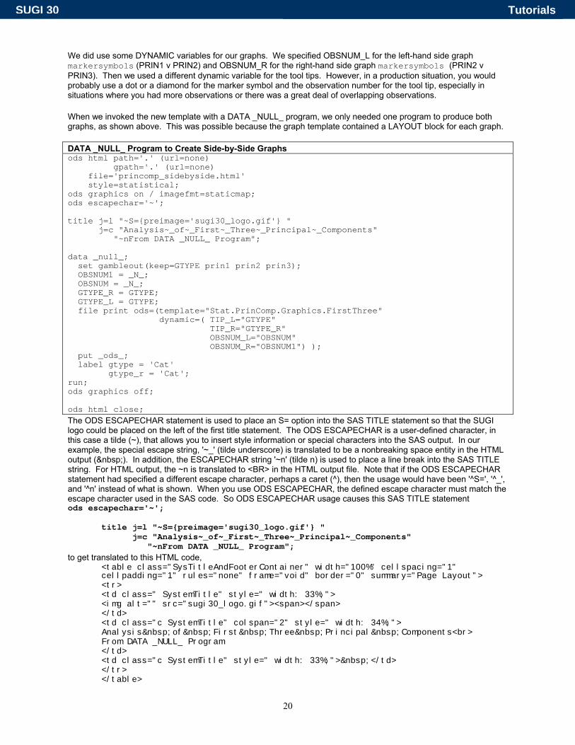
We did use some DYNAMIC variables for our graphs. We specified OBSNUM_L for the left-hand side graph markersymbols (PRIN1 v PRIN2) and OBSNUM_R for the right-hand side graph markersymbols (PRIN2 v PRIN3). Then we used a different dynamic variable for the tool tips. However, in a production situation, you would probably use a dot or a diamond for the marker symbol and the observation number for the tool tip, especially in situations where you had more observations or there was a great deal of overlapping observations. When we invoked the new template with a DATA _NULL_ program, we only needed one program to produce both graphs, as shown above. This was possible because the graph template contained a LAYOUT block for each graph. DATA _NULL_ Program to Create Side-by-Side Graphs ods html path='.' (url=none) gpath='.' (url=none) file='princomp_sidebyside.html' style=statistical; ods graphics on / imagefmt=staticmap; ods escapechar='~'; title j=l "~S={preimage='sugi30_logo.gif'} " j=c "Analysis~_of~_First~_Three~_Principal~_Components" "~nFrom DATA _NULL_ Program"; data _null_; set gambleout(keep=GTYPE prin1 prin2 prin3); OBSNUM1 = _N_; OBSNUM = _N_; GTYPE_R = GTYPE; GTYPE_L = GTYPE; file print ods=(template="Stat.PrinComp.Graphics.FirstThree" dynamic=( TIP_L="GTYPE" TIP_R="GTYPE_R" OBSNUM_L="OBSNUM" OBSNUM_R="OBSNUM1") ); put _ods_; label gtype = 'Cat' gtype_r = 'Cat'; run; ods graphics off; ods html close; The ODS ESCAPECHAR statement is used to place an S= option into the SAS TITLE statement so that the SUGI logo could be placed on the left of the first title statement. The ODS ESCAPECHAR is a user-defined character, in this case a tilde (~), that allows you to insert style information or special characters into the SAS output. In our example, the special escape string, '~_' (tilde underscore) is translated to be a nonbreaking space entity in the HTML output (&nbsp;). In addition, the ESCAPECHAR string '~n' (tilde n) is used to place a line break into the SAS TITLE string. For HTML output, the ~n is translated to <BR> in the HTML output file. Note that if the ODS ESCAPECHAR statement had specified a different escape character, perhaps a caret (^), then the usage would have been '^S=', '^_', and '^n' instead of what is shown. When you use ODS ESCAPECHAR, the defined escape character must match the escape character used in the SAS code. So ODS ESCAPECHAR usage causes this SAS TITLE statement ods escapechar='~';

title j=l "~S={preimage='sugi30_logo.gif'} " j=c "Analysis~_of~_First~_Three~_Principal~_Components" "~nFrom DATA _NULL_ Program";

to get translated to this HTML code, <table class="SysTitleAndFooterContainer" width="100%" cellspacing="1" cellpadding="1" rules="none" frame="void" border="0" summary="Page Layout"> <tr> <td class=" SystemTitle" style=" width: 33%;"> <img alt="" src="sugi30_logo.gif"><span></span> </td> <td class="c SystemTitle" colspan="2" style=" width: 34%;"> Analysis&nbsp;of&nbsp;First&nbsp;Three&nbsp;Principal&nbsp;Components<br> From DATA _NULL_ Program </td> <td class="c SystemTitle" style=" width: 33%;">&nbsp;</td> </tr> </table>

SUGI 30 Tutorials

21

in the HTML output file. We used the nonbreaking space escape character to cause the entire title to be treated as one continuous string. And we used the pre-image style attribute to cause the SUGI logo GIF file to be used in the <IMG> tag. Note how the pre-image style attribute uses a simple filename and extension. This is called a 'relative' reference for the SRC= option. For this technique to work, the GIF file and the HTML file must be placed in the same directory on your local machine or on your Web server. You can gain more knowledge about style templates, table templates, and ODS ESCAPECHAR from the Education Division class "Advanced Output Delivery System Topics," which is available as either classroom training or as Live Web training. Currently, this class does not cover ODS Graphics topics. In the future, if demand warrants, we will develop training on ODS Graphics subjects. However, we hope that we have shown that usage of ODS Graphics spans a continuum from very easy, with no extra code except ODS GRAPHICS ON/OFF statements, to extremely customized, through the use of graph template syntax and style template syntax, along with DATA _NULL_ programming and other ODS components.

CONCLUSION In conclusion, we'd like to enthusiastically reiterate our earlier statement that ODS statistical graphics capability represents an exciting new feature of SAS®9. With ODS Graphics, analytical procedures in SAS can create professional-quality graphics either automatically or with a minimal number of options. The automatic graphs generated are sufficient for most data analytic situations, in which case the templates will not need modification. However, if you do need to make persistent graph changes, we hope that our exploration of the interactions between the graph templates, style templates, and other ODS components will make your job easier.

ACKNOWLEDGMENTS The authors would like to thank Michele Ensor, Jeff Cartier, Sanjay Matange, Tonya Balan, Bob Rodriguez, and the rest of the data visualization group for their help and suggestions on how to improve this paper.

REFERENCES For more information about Graph Templates and Graph Template Language, consult the ODS documentation at the Web site http://support.sas.com/91doc/getDoc/statug.hlp/odsgraph_sect23.htm. In addition, these papers were very useful for research into the behavior of Graph templates: Proceedings of the Annual Conference of the SAS Users Group International. Cary, NC: SAS Institute Inc. Cartier, J.: "Graphs In Style" (SUGI 29). Cartier, J.: "It's All in the Presentation" (SUGI 28). Rodriguez, R. “An Introduction to ODS for Statistical Graphics in SAS 9.1” (SUGI 29). Other papers: Cartier, J.: "Visual Styles for V9 SAS Output." <http://support.sas.com/rnd/datavisualization/papers/VisualStyles.pdf>. Okerson, B.: "Evaluating Hospital Performance: Using SAS ODS to Create a Hospital Scorecard." <http://www2.sas.com/proceedings/sugi29/157-29.pdf>.

APPENDIX The ODS Graphics programs provided here are coded using the experimental syntax specific to SAS 9.1.3 ODS Graphics features. These programs are provided "as is" and are not intended to be used in a production environment. They are provided for experimentation and learning purposes only. Please note that the syntax for Graph templates will change in a future release and the syntax shown in these programs may no longer be valid.

PROGRAM: DEMO2_ODSGRAF.SAS PROGRAM: DEMO4_SELECT.SAS options nodate pageno=1; ods listing close; ** PROC PRINCOMP and the; ** default ODS output. ; ods path sashelp.tmplmst(read); ods html path='.' (url=none) gpath='.' (url=none) file='princomp_default.html' style=statistical; ods graphics on / imagefmt=staticmap; proc princomp data = work.gamblegrp cov std; title 'Default PRINCOMP Output';

options nodate pageno=1; ods listing close; ** PROC PRINCOMP and the; ** default ODS output. ; ** Using ODS SELECT to get; ** PRIN1 v PRIN2 and ** PRIN1 v PRIN3; ods path sashelp.tmplmst(read); ods html path='.' (url=none) gpath='.' (url=none) file='princomp_select.html' style=statistical; ods select PrinCompScoresPlot12 PrinCompScoresPlot13;

SUGI 30 Tutorials

22

var dsm1-dsm12; run; ods graphics off; ods html close; title;

ods graphics on / imagefmt=staticmap; proc princomp data = work.gamblegrp cov std; title 'Default PRINCOMP Output + SELECT'; var dsm1-dsm12; run; ods graphics off; ods html close;

NOTE Because the remaining program samples are lengthy, they are available for download as a Zip file from the following Web site: http://support.sas.com/rnd/papers/index.html . Alternately, if you are unable to download Zip files, but can receive Zip files as e-mail attachments, you may e-mail the authors after the SUGI conference to have the program files for this paper e-mailed to you.

CONTACT INFORMATION Contact the authors at

Catherine Truxillo SAS Institute SAS Campus Drive Cary, NC 27513 919-531-4641 Catherine.Truxillo@sas.com

Cynthia Zender SAS Institute Denver, CO 303-290-9112 ext 1738 Cynthia.Zender@sas.com

SAS and all other SAS Institute Inc. product or service names are registered trademarks or trademarks of SAS Institute Inc. in the USA and other countries. ® indicates USA registration. Other brand and product names are trademarks of their respective companies.

SUGI 30 Tutorials