1

Paper 236-30

Data Step Hash Objects as Programming Tools

Paul M. Dorfman, Independent Consultant, Jacksonville, FL Koen Vyverman, SAS Netherlands

ABSTRACT In SAS® Version 9.1, the hash table - the very first object introduced via the Data Step Component Interface in Version 9.0 - has become robust and syntactically stable. The philosophy and application style of the hash objects differs quite radically from any other structure ever used in the Data step previously. The most notable departure from the tradition is their run-time nature. The hash objects are instantiated and/or deleted and acquire memory, if necessary, at the run-time. It is intuitively clear that such traits should make for very interesting and flexible programming having not seen in the Data step code of yore. Although some propaedeutics will be provided in the paper, the talk is intended for SAS programmers already somewhat familiar with the basic ideas and syntax behind the hash objects. Instead of teaching hash basics - which by now has been rehashed enough! – live code examples will be used to demonstrate a number of programming techniques, which would be utterly unthinkable before the advent of the canned hash objects in SAS. Imagine using “data _null_” to write a SAS data set, whose name depends on a variable. Or fancy sorting a huge temporary array rapidly and efficiently without the need for sophisticated hand-coding. In other words, you are in for a few intriguing SAS tunes from the hash land. INTRODUCTION In the title of the paper, the term “hashing” was used collectively to denote the whole group of memory-resident searching methods not primarily based on comparison between keys, but on direct addressing. Although hashing per se is, strictly speaking, merely one of direct-addressing techniques, using the word as a collective term has become quite common. Hopefully, it will be clear from the context in which sense the term is used. Mostly, it will be used in its strict meaning. From the algorithmic standpoint, hashing is by no means a novel scheme, nor it is new in the SAS land. In fact, a number of direct-addressing searching techniques have been successfully implemented using the Data step language and shown to be practically useful! This set of hand-coded direct-addressing routines, together with a rather painful delving into their guts, was presented at SUGI 26 and 27 [1, 2]. Hand-coded methods have a number of drawbacks – inevitable for almost any more or less complex, performance-oriented routine coded in a very high-level language, such as the SAS Data step. But it has a number of advantages as well, primarily that the code is available, and so it can be tweaked to anyone’s liking, changed to accommodate different specifications, retuned, etc. SAS Version 9 has introduced many new features into the Data step language. Most of them expand existing functionality and/or improve performance, and thus are rather incremental. However, one novel concept stands out as a breakthrough: The Data step Component Interface. The two first objects available through this interface to a Data step programmer are associative array (or hash object) and the associated hash iterator object. These objects can be used as a memory-resident dynamic Data step dictionaries, which can be created and deleted at the run time and perform the standard operations of finding, adding, and removing data practically in O(1) time. Being adroitly implemented in the underlying SAS software, these modules are quite fast, and the fact that memory they need to store data is allocated dynamically, at the run time, makes the hash objects a real breakthrough. HASH OBJECT AB OVO BY EXAMPLE: FILE MATCHING Perhaps the best way to get a fast taste of this mighty addition to the Data step family is to see how easily it can help solve the “matching problem”. Suppose we have a SAS file LARGE with $9 character key KEY, and a file SMALL with a similar key and some additional info stored in a numeric variable S_SAT. We need to use the SMALL file as a fast lookup

SUGI 30 Tutorials

2

table to pull S_SAT into LARGE for each KEY having a match in SMALL. This step shows one way how the hash (associative array) object can help solve the problem: Example 1: File Matching (Lookup file loaded in a loop) data match ( drop = rc ) ; length key $9 s_sat 8 ; declare AssociativeArray hh () ; rc = hh.DefineKey ( 'key' ) ; rc = hh.DefineData ( 's_sat' ) ; rc = hh.DefineDone () ; do until ( eof1 ) ; set small end = eof1 ; rc = hh.add () ; end ; do until ( eof2 ) ; set large end = eof2 ; rc = hh.find () ; if rc = 0 then output ; end ; stop ; run ; After all the trials and tribulations of coding hashing algorithms by hand, this simplicity looks rather stupefying. But how does this code go about its business? • LENGTH statement gives SAS the attributes of the key and data elements before the methods defining them could be

called. • DECLARE AssociativeArray statement declares and instantiates the associative array (hash table) HH. • DefineKey method describes the variable(s) to serve as a key into the table. • DefineData method is called if there is a non-key satellite information, in this case, S_SAT, to be loaded in the table. • DefineDone method is called to complete the initialization of the hash object. • ADD method grabs a KEY and S_SAT from SMALL and loads both in the table. Note that for any duplicate KEY coming

from SMALL, ADD() will return a non-zero code and discard the key, so only the first instance the satellite corresponding to a non-unique key will be used.

• FIND method searches the hash table HH for each KEY coming from LARGE. If it is found, the return code is set to zero, and host S_SAT field is updated with its value extracted from the hash table.

If you think it is prorsus admirabile, then the following step does the same with even less coding: Example 2: File Matching (Lookup file is loaded via the DATASET: parameter) data match ; set small point = _n_ ; * get key/data attributes for parameter type matching ; * set small (obs = 1) ; * this will work, too :-)! ; * if 0 then set small ; * and so will this :-)! ; * set small (obs = 0) ; * but for some reason, this will not :-( ; dcl hash hh (dataset: 'work.small', hashexp: 10) ; hh.DefineKey ( 'key' ) ; hh.DefineData ( 's_sat' ) ; hh.DefineDone () ; do until ( eof2 ) ; set large end = eof2 ; if hh.find () = 0 then output ; end ; stop ; run ;

SUGI 30 Tutorials

3

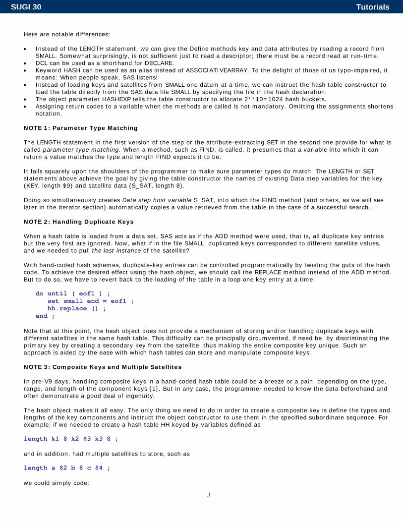
Here are notable differences: • Instead of the LENGTH statement, we can give the Define methods key and data attributes by reading a record from

SMALL. Somewhat surprisingly, is not sufficient just to read a descriptor; there must be a record read at run-time. • DCL can be used as a shorthand for DECLARE. • Keyword HASH can be used as an alias instead of ASSOCIATIVEARRAY. To the delight of those of us typo-impaired, it

means: When people speak, SAS listens! • Instead of loading keys and satellites from SMALL one datum at a time, we can instruct the hash table constructor to

load the table directly from the SAS data file SMALL by specifying the file in the hash declaration. • The object parameter HASHEXP tells the table constructor to allocate 2**10=1024 hash buckets. • Assigning return codes to a variable when the methods are called is not mandatory. Omitting the assignments shortens

notation. NOTE 1: Parameter Type Matching The LENGTH statement in the first version of the step or the attribute-extracting SET in the second one provide for what is called parameter type matching. When a method, such as FIND, is called, it presumes that a variable into which it can return a value matches the type and length FIND expects it to be. It falls squarely upon the shoulders of the programmer to make sure parameter types do match. The LENGTH or SET statements above achieve the goal by giving the table constructor the names of existing Data step variables for the key (KEY, length $9) and satellite data (S_SAT, length 8). Doing so simultaneously creates Data step host variable S_SAT, into which the FIND method (and others, as we will see later in the iterator section) automatically copies a value retrieved from the table in the case of a successful search. NOTE 2: Handling Duplicate Keys When a hash table is loaded from a data set, SAS acts as if the ADD method were used, that is, all duplicate key entries but the very first are ignored. Now, what if in the file SMALL, duplicated keys corresponded to different satellite values, and we needed to pull the last instance of the satellite? With hand-coded hash schemes, duplicate-key entries can be controlled programmatically by twisting the guts of the hash code. To achieve the desired effect using the hash object, we should call the REPLACE method instead of the ADD method. But to do so, we have to revert back to the loading of the table in a loop one key entry at a time: do until ( eof1 ) ; set small end = eof1 ; hh.replace () ; end ; Note that at this point, the hash object does not provide a mechanism of storing and/or handling duplicate keys with different satellites in the same hash table. This difficulty can be principally circumvented, if need be, by discriminating the primary key by creating a secondary key from the satellite, thus making the entire composite key unique. Such an approach is aided by the ease with which hash tables can store and manipulate composite keys. NOTE 3: Composite Keys and Multiple Satellites In pre-V9 days, handling composite keys in a hand-coded hash table could be a breeze or a pain, depending on the type, range, and length of the component keys [1]. But in any case, the programmer needed to know the data beforehand and often demonstrate a good deal of ingenuity. The hash object makes it all easy. The only thing we need to do in order to create a composite key is define the types and lengths of the key components and instruct the object constructor to use them in the specified subordinate sequence. For example, if we needed to create a hash table HH keyed by variables defined as length k1 8 k2 $3 k3 8 ; and in addition, had multiple satellites to store, such as length a $2 b 8 c $4 ; we could simply code:

SUGI 30 Tutorials

4

dcl hash hh () ; hh.DefineKey ('k1', 'k2', 'k3') ; hh.DefineData ('a', 'b', 'c') ; hh.DefineDone () ; and the internal hashing scheme will take due care about whatever is necessary to come up with a hash bucket number where the entire composite key should fall together with its satellites. Multiple keys and satellite data can be loaded into a hash table one element at a time by using the ADD or REPLACE methods. For example, for the table defined above, we can value the keys and satellites first and then call the ADD or REPLACE method: k1 = 1 ; k2 = 'abc' ; k3 = 3 ; a = 'a1' ; b = 2 ; c = 'wxyz' ; rc = hh.replace () ; k1 = 2 ; k2 = 'def' ; k3 = 4 ; a = 'a2' ; b = 5 ; c = 'klmn' ; rc = hh.replace () ; Alternatively, these two table entries can be coded as hh.replace (key: 1, key: 'abc', key: 3, data: 'a1', data: 2, data: 'wxyz') ; hh.replace (key: 2, key: 'def', key: 4, data: 'a2', data: 5, data: 'klmn') ; Note that more that one hash table entry cannot be loaded in the table at compile-time at once, as it can be done in the case of arrays. All entries are loaded one entry at a time at run-time. Perhaps it is a good idea to avoid hard-coding data values in a Data step altogether, and instead always load them in a loop either from a file or, if need be, from arrays. Doing so reduces the propensity of the program to degenerate into an object Master Ian Whitlock calls “wall paper”, and helps separate code from data. NOTE 4: Hash Object Parameters as Expressions The two steps above may have already given a hash-hungry reader enough to start munching overwhelming programming opportunities opened by the availability of the SAS-prepared hash food without the necessity to cook it. To add a little more spice to it, let us rewrite the step yet another time: Example 3: File Matching (Using expressions for parameters) data match ; set small (obs = 1) ; retain dsn ‘small’ x 10 kn ‘key’ dn ‘s_sat’ ; dcl hash hh (dataset: dsn, hashexp: x) ; hh.DefineKey ( kn ) ; hh.DefineData ( dn ) ; hh.DefineDone ( ) ; do until ( eof2 ) ; set large end = eof2 ; if hh.find () = 0 then output ; end ; stop ; run ;

SUGI 30 Tutorials

5

As we see, the parameters passed to the constructor (such as DATASET and HASHEXP) and methods need not necessarily be hard-coded literals. They can be passed as valued Data step variables, or even as appropriate type expressions. For example, it is possible to code (if need be): retain args ‘small key s_sat’ n_keys 1e6; dcl hash hh ( dataset: substr(args,1,5) hashexp: log2(n_keys) ) ; hh.DefineKey ( scan(s, 2) ) ; hh.DefineData ( scan(s,-1) ) ; hh.DefineDone ( ) ; HITER: HASH ITERATOR OBJECT During both hash table load and look-up, the sole question we need to answer is whether the particular search key is in the table or not. The FIND and CHECK hash methods give the answer without any need for us to know what other keys may or may not be stored in the table. However, in a variety of situations we do need to know the keys and data currently resident in the table. How do we do that? In hand-coded schemes, it is simple since we had full access to the guts of the table. However, hash object entries are not accessible as directly as array entries. To make them accessible, SAS provides the hash iterator object, hiter, which makes the hash table entries available in the form of a serial list. Let us consider a simple program that should make it all clear: Example 4: Dumping the Contents of an Ordered Table Using the Hash Iterator data sample ; input k sat ; cards ; 185 01 971 02 400 03 260 04 922 05 970 06 543 07 532 08 050 09 067 10 ; run ; data _null_ ; if 0 then set sample ; dcl hash hh ( dataset: 'sample', hashexp: 8, ordered: 'a') ; dcl hiter hi ( 'hh' ) ; hh.DefineKey ( 'k' ) ; hh.DefineData ( 'sat' , 'k' ) ; hh.DefineDone () ; do rc = hi.first () by 0 while ( rc = 0 ) ; put k = z3. +1 sat = z2. ; rc = hi.next () ; end ; put 13 * '-' ; do rc = hi.last () by 0 while ( rc = 0 ) ;

SUGI 30 Tutorials

6

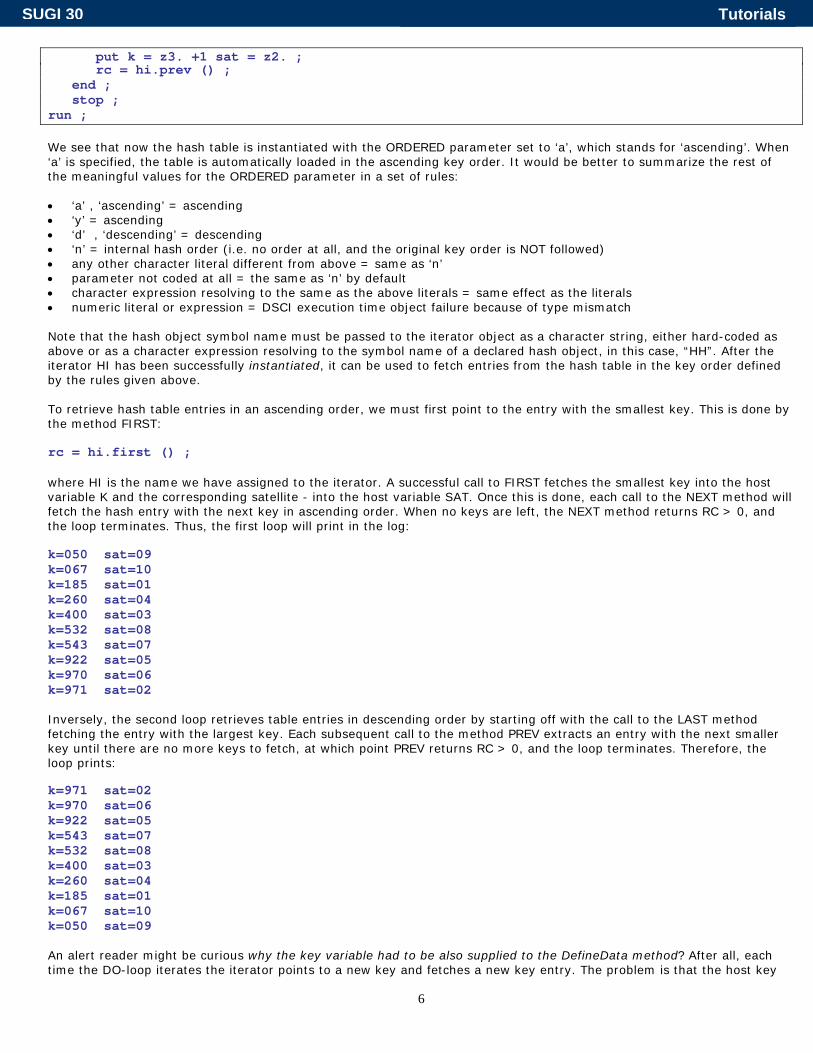
put k = z3. +1 sat = z2. ; rc = hi.prev () ; end ; stop ; run ; We see that now the hash table is instantiated with the ORDERED parameter set to ‘a’, which stands for ‘ascending’. When ‘a’ is specified, the table is automatically loaded in the ascending key order. It would be better to summarize the rest of the meaningful values for the ORDERED parameter in a set of rules: • ‘a’ , ‘ascending’ = ascending • ‘y’ = ascending • ‘d’ , ‘descending’ = descending • ‘n’ = internal hash order (i.e. no order at all, and the original key order is NOT followed) • any other character literal different from above = same as ‘n’ • parameter not coded at all = the same as ‘n’ by default • character expression resolving to the same as the above literals = same effect as the literals • numeric literal or expression = DSCI execution time object failure because of type mismatch Note that the hash object symbol name must be passed to the iterator object as a character string, either hard-coded as above or as a character expression resolving to the symbol name of a declared hash object, in this case, “HH”. After the iterator HI has been successfully instantiated, it can be used to fetch entries from the hash table in the key order defined by the rules given above. To retrieve hash table entries in an ascending order, we must first point to the entry with the smallest key. This is done by the method FIRST: rc = hi.first () ; where HI is the name we have assigned to the iterator. A successful call to FIRST fetches the smallest key into the host variable K and the corresponding satellite - into the host variable SAT. Once this is done, each call to the NEXT method will fetch the hash entry with the next key in ascending order. When no keys are left, the NEXT method returns RC > 0, and the loop terminates. Thus, the first loop will print in the log: k=050 sat=09 k=067 sat=10 k=185 sat=01 k=260 sat=04 k=400 sat=03 k=532 sat=08 k=543 sat=07 k=922 sat=05 k=970 sat=06 k=971 sat=02 Inversely, the second loop retrieves table entries in descending order by starting off with the call to the LAST method fetching the entry with the largest key. Each subsequent call to the method PREV extracts an entry with the next smaller key until there are no more keys to fetch, at which point PREV returns RC > 0, and the loop terminates. Therefore, the loop prints: k=971 sat=02 k=970 sat=06 k=922 sat=05 k=543 sat=07 k=532 sat=08 k=400 sat=03 k=260 sat=04 k=185 sat=01 k=067 sat=10 k=050 sat=09 An alert reader might be curious why the key variable had to be also supplied to the DefineData method? After all, each time the DO-loop iterates the iterator points to a new key and fetches a new key entry. The problem is that the host key

SUGI 30 Tutorials

7

variable K is updated only once, as a result of the HI.FIRST() or HI.LAST() method call. Calls to PREV and NEXT methods do not update the host key variable. However, a satellite hash variable does! So, if in the step above, it had not been passed to the DefineData method as an additional argument, only the key values 050 and 971 would have been printed. The concept behind such behavior is that only data entries in the table have the legitimate right to be “projected” onto its Data step host variables, whilst the keys do not. It means that if you need the ability to retrieve a key from a hash table, you need to define it in the data portion of the table as well. NOTE 5: Array Sorting via a Hash Iterator The ability of a hash iterator to rapidly retrieve hash table entries in order is an extremely powerful feature, which will surely find a lot of use in Data step programming. The first iterator programming application that springs to mind immediately is using its key ordering capabilities to sort another object. The easiest and most apparent prey is a SAS array. The idea of sorting an array using the hash iterator is very simple: 1. Declare an ordered hash table keyed by a variable of the data type and length same as those of the array. 2. Declare a hash iterator. 3. Assign array items one at a time to the key and insert the key in the table. 4. Use the iterator to retrieve the keys one by one from the table and repopulate the array, now in order. A minor problem with this most brilliant plan, though, is that since the hash object table cannot hold duplicate keys, a certain provision ought to be made in the case the when the array contains duplicate elements. The simplest way to account for duplicate array items is to enumerate the array as it is used to load the table and use the unique enumerating variable as an additional key into the table. In the case the duplicate elements need to be eliminated from the array, the enumerating variable can be merely set to a constant, which below is chosen to be a zero: Example 5: Using the Hash Iterator to Sort an Array data _null_ ; array a [-100000 : 100000] _temporary_ ; ** allocate sample array with random numbers, about 10 percent duplicate ; do _q = lbound (a) to hbound (a) ; a [_q] = ceil (ranuni (1) * 2000000) ; end ; ** set sort parameters ; seq = 'A' ; * A = ascending, D = descending ; nodupkey = 0 ; * 0 = duplicates allowed, 1 = duplicates not allowed ; dcl hash _hh (hashexp: 0, ordered: seq) ; dcl hiter _hi ('_hh' ) ; _hh.definekey ('_k', '_n' ) ; * _n - extra enumerating key ; _hh.definedata ('_k' ) ; * _k automatically assumes array data type ; _hh.definedone ( ) ; ** load composite (_k _n) key on the table ; ** if duplicates to be retained, set 0 <- _n ; do _j = lbound (a) to hbound (a) ; _n = _j * ^ nodupkey ; _k = a [_j] ; _hh.replace() ; end ; ** use iterator HI to reload array from HH table, now in order ; _n = lbound (a) - 1 ; do _rc = _hi.first() by 0 while ( _rc = 0 ) ; _n = _n + 1 ;

SUGI 30 Tutorials

8

a [_n] = _k ; _rc = _hi.next() ; end ; _q = _n ; ** fill array tail with missing values if duplicates are delete ; do _n = _q + 1 to hbound (a) ; a [_n] = . ; end ; drop _: ; * drop auxiliary variables ; ** check if array is now sorted ; sorted = 1 ; do _n = lbound (a) + 1 to _q while ( sorted ) ; if a [_n - 1] > a [_n] then sorted = 0 ; end ; put sorted = ; run ; Note that choosing HASHEXP:16 above would be more beneficial performance-wise. However, HASHEXP=0 was chosen to make an important point a propos: Since it means 2**0=1, i.e. a single bucket, we have created a stand-alone AVL(Adelson-Volsky & Landis) binary tree in a Data step, let it grow dynamically as it was being populated with keys and satellites, and then traversed it to eject the data in a predetermined key order. So, do not let anyone tell you that a binary search tree cannot be created, dynamically grown and shrunk, and deleted, as necessary at the Data step run time. It can, and with very a little programmatic effort, too! Just to give an idea about this hash table performance in some absolute figures, this entire step runs in about 1.15 seconds on a desktop 933 MHz computer under XP Pro. The time is pretty deceiving, since 85 percent of it is spent inserting the data in the tree. The process of sorting 200,001 entries itself takes only scant 0.078 seconds either direction. Increasing HASHEXP to 16 reduces the table insertion time by about 0.3 seconds, while the time of dumping the table in order remains the same. One may ask why bother to program array sorting, even if the program is as simple and transparent as above, if in Version 9, CALL SORT() routine exists seemingly for the same purpose. In actuality, CALL SORT() is designed to sort variable lists, which may or may not be organized into arrays. As such, it does not allow the provision of sorting a temporary array by a single array reference, unless all of its elements are explicitly listed. Of course, it is possible to assemble the references one by one using a macro or another technique, but with 200001 elements to sort, it takes over 30 seconds just to compile the step. Besides, such method does not allow accounting for duplicates, and for those who care about such things, looks aesthetically maladroit. DATA STEP COMPONENT INTERFACE Now that we have a taste of the new Data step hash objects and some cool programming tricks they can be used to pull, let us consider it from a little bit more general viewpoint. In Version 9, the hash table (associative array) introduces the first component object accessible via a rather novel thingy called DATA Step Component Interface (DSCI). A component object is an abstract data entity consisting of two distinct characteristics: Attributes and methods. Attributes are data that the object can contain, and methods are operations the object can perform on its data. From the programming standpoint, an object is a black box with known properties, much like a SAS procedure. However, a SAS procedure, such as SORT or FORMAT, cannot be called from a Data step at run-time, while an object accessible through DSCI - can. A Data step programmer who wants an object to perform some operation on its data, does not have to program it procedurally, but only to call an appropriate method. The Hash Object In our case, the object is a hash table. Generally speaking, as an abstract data entity, a hash table is an object providing for the insertion and retrieval of its keyed data entries in O(1), i.e. constant, time. Properly built direct-addressed tables

SUGI 30 Tutorials

9

ject must be eclared. In other words, the hash table must be instantiated with the DECLARE (DCL) statement, as we have seen above.

satisfy this definition in the strict sense. We will see that the hash object table satisfies it in the practical sense. The attributes of the hash table object are keyed entries comprising its key(s) and maybe also satellites. Before any hash table object methods can be called (operations on the hash entries performed), the obd The hash table methods are the functions it can perform, namely: • DefineKey. Define a set of hash keys. • DefineData. Define a set of hash table satellites. This method call can be omitted without harmful consequences if

e table. Although a dummy call can still be issued, it is not required. there is no need for non-key data in th• DefineDone. Tell SAS the definitions are done. If the DATASET argument is passed to the table’s definition, load the

table from the data set.

• ADD. Insert the key and satellites if the key is not yet in the table (ignore duplicate keys). • REPLACE. If the key is not in the table, insert the key and its satellites, otherwise overwrite the satellites in the table

for this key with new ones. • REMOVE. Delete the entire entry from the table, including the key and the data. • FIND. Search for the key. If it is found, extract the satellite(s) from the table and update the host Data step variables. • CHECK. Search for the key. If it is found, just return RC=0, and do nothing more. Note that calling this method does

not overwrite the host variables. • OUTPUT. Dump the entire current contents of the table into a one or more SAS data set. Note that for the key(s) to

dumped, they must be defined using the DefineData method. If the table has been loaded in order, it will be dumped

Dat

a method, we only have to specify its name preceded by the name of the object followed y a period, such as:

anner of telling SAS Data step what to do is thus naturally called the Data Step Object Dot Syntax. des a linguistic access to a component object’s methods and attributes.

t DSCI. The compiler cognizes the syntax, and it reacts harshly if the dot syntax is present, but the object to which it is apparently applied is

also in order. More information about the method will be provided later on.

a Step Object Dot Syntax As we have seen, in order to call b hh.DefineKey () hh.Find () hh.Replace () hh.First () hh.Output () and so on. This mummarily, it proviS

Note that the object dot syntax is one of very few things the Data step compiler knows aboureabsent. For example, an attempt to compile this step, data _null_ ;

Component Object failure. Aborted during the COMPILATION phase.

is not an object.

ta step through DSCI. However, as their number grows, we ntax really soon, particularly those dinosaurs among us who have not exactly

hh.DefineKey ('k') ; run ;

sage from the compiler (not from the object): results in the following log mes 6 data _null_ ; ERROR: DATA STEP 7 hh.DefineKey ('k') ; ------------ 557

e hh ERROR 557-185: Variabl8 run ;

w component objects are accessible from a DaSo far, just a fead better get used to the object dot syh

learned this kind of tongue in the kindergarten... A PEEK UNDER THE HOOD

SUGI 30 Tutorials

10

We have just seen the tip of the hash iceberg from the outside. An inquiring mind would like to know: What is inside? Not that we really need the gory details of the underlying code, but it is instructive to know on which principles the design of the internal SAS table is based in general. A good driver is always curious what is under the hood. Well, in general, hashing is hashing is hashing - which means that it is always a two-staged process: 1) Hashing a key to its bucket 2) resolving collisions within each bucket. Hand-coded hashing cannot rely on the simple straight separate chaining because of the inability to dynamically allocate memory one entry at a time, while reserving it in advance could result in unreasonable waste of memory. Since the hash and hiter objects are coded in the underlying software, this restriction no longer exists, and so separate chaining is perhaps the most logical way to go. Its concrete implementation, however, has somewhat deviated from the classic scheme of connecting keys within each node into a link list. Instead, each new key hashing to a bucket is inserted into its binary tree. If there were, for simplicity, only 4 buckets, the scheme might roughly look like this: 0 1 2 3 +---------+---------+---------+---------+ | | | | | | | | | | / \ | / \ | / \ | / \ | | /\ /\ | /\ /\ | /\ /\ | /\ /\ | The shrub-like objects inside the buckets are AVL (Adelson-Volsky & Landis) trees. AVL trees are binary trees populated by such a mechanism that on the average guarantees their O(log(N)) search behavior regardless of the distribution of the key values. The number of hash buckets is controlled by the HASHEXP parameter we have used above. The number of buckets allocated by the hash table constructor is 2**HASHEXP. So, if HASHEXP=8, HZISE=256 buckets will be allocated, or if HASHEXP=16, HSIZE=65536. As of the moment, it is the maximum. Any HASHSIZE specified over 16 is truncated to 16. Let us assume HASHEXP=16 and try to see how, given a KEY, this structure facilitates hashing. First, a mysterious internal hash function maps the key, whether is it simple or composite, to some bucket. The tree in the bucket is searched for KEY. If it is not there, the key and its satellite data are inserted in the tree. If KEY is there, it is either discarded when ADD is called, or its satellite data are updated when REPLACE is called. Just how fast all this occurs depends on the speed of search. Suppose that we have N=2**20, i.e. about 1 million keys. With HSIZE=2**16, there will be on the average 2**4 = 16 keys hashing to one bucket. Since N > HSIZE, the table is overloaded, i.e. its load factor is greater than 1. However, binary searching the 16 keys in the AVL tree requires only about 5 keys comparisons. If we had 10 million keys, it would require about 7 comparisons, which practically makes almost no difference. Thus, the SAS object hash table behaves as O(log(N/HSIZE)). While it is not exactly O(1), it can be considered such for all practical intents and purposes, as long as N/HSIZE is not way over 100. Thus, by choosing HASHEXP judiciously, it is thus possible to tweak the hash table performance to some degree and depending on the purpose. For example, if the table is used primarily for high-performance matching, it may be a good idea to specify the maximum HASHEXP=16, even if some buckets end up unused. From our preliminary testing, we have not been able to notice any memory usage penalty exacted by going to the max, all the more that as of this writing, the Data step does not seem to report memory used by an object called through the DSCI. At least, experiments with intentionally large hash tables show that the memory usage reported in the log is definitely much smaller than the hash table must have occupied, although it was evident from performance that the table is completely memory-resident, and the software otherwise has no problem handling it. However, with several thousand keys at hand there is little reason to go over HASHEXP=10, anyway. Also, if the sole purpose of using the table is to eject the data in a key order using a hash iterator, even a single bucket at HASHEXP=0 can do just fine, as we saw earlier with the array sorting example. On the other hand, if there is no need for iterator processing, it is better to leave the table completely iterator-free by not specifying a non-zero ORDERED option. Maintaining an iterator over a hash table obviously requires certain overhead. HASH TABLE AS A DYNAMIC DATA STEP STRUCTURE The hash table object (together with its hiter sibling) represents the first ever dynamic Data step structure, i.e. one capable of acquiring memory and growing at run-time. There are a number of common situations in data processing when the information needed to size a data structure becomes available only at execution time. SAS programmers usually solve such problems by pre-processing data, either i.e. passing through the data more than once, or allocating memory resources for the worst-case scenario. As more programmers become familiar with the possibilities this dynamic structure offers, they will be able to avoid resorting to many old kludges.

SUGI 30 Tutorials

11

Remember, a hash object is instantiated during the run-time. If the table is no longer needed, it can be simply wiped out by the DELETE method: rc = hh.Delete () ; This will eliminate the table from memory for good, but not its iterator! As a separate object related to a hash table, it has to be deleted separately: rc = hi.Delete () ; If at some point of a Data step program there is a need to start building the same table from scratch again, remember that the compiler must see only a single definition of the same table by the same token as it must see only a single declaration of the same array (and if the rule is broken, it will issue the same error message, e.g.: “Variable hh already defined”). Also, like in the case of arrays, the full declaration (table and its iterator) must precede any table/iterator references. In other words, this will NOT compile because of the repetitive declaration: 20 data _null_ ; 21 length k 8 sat $11 ; 22 23 dcl hash hh ( hashexp: 8, ordered: 1 ) ; 24 dcl hiter hi ( 'hh' ) ; 25 hh.DefineKey ( 'k' ) ; 26 hh.DefineData ( 'sat' ) ; 27 hh.DefineDone () ; 28 29 hh.Delete () ; 30 31 dcl hash hh (hashexp: 8, ordered: 1 ) ; - 567 ERROR 567-185: Variable hh already defined. 32 dcl hiter hi ( 'hh' ) ; - 567 ERROR 567-185: Variable hi already defined. And this will not compile because at the time of the DELETE method call, the compiler has not seen HH yet: 39 data _null_ ; 40 length k 8 sat $11 ; 41 link declare ; 42 rc = hh.Delete() ; --------- 557 68 ERROR 557-185: Variable hh is not an object. ERROR 68-185: The function HH.DELETE is unknown, or cannot be accessed. 43 link declare ; 44 stop ; 45 declare: 46 dcl hash hh ( hashexp: 8, ordered: 1 ) ; 47 dcl hiter hi ( 'hh' ) ; 48 hh.DefineKey ( 'k' ) ; 49 hh.DefineData ( 'sat' ) ; 50 hh.DefineDone () ; 51 return ; 52 stop ; 53 run ; However, if we do not dupe the compiler and reference the object after it has seen it, it will work as designed:

SUGI 30 Tutorials

12

199 data _null_ ; 200 retain k 1 sat 'sat' ; 201 if 0 then do ; 202 declare: 203 dcl hash hh ( hashexp: 8, ordered: 1 ) ; 204 dcl hiter hi ( 'hh' ) ; 205 hh.DefineKey ( 'k' ) ; 206 hh.DefineData ( 'sat' ) ; 207 hh.DefineDone () ; 208 return ; 209 end ; 210 link declare ; 211 rc = hi.First () ; 212 put k= sat= ; 213 rc = hh.Delete () ; 214 rc = hi.Delete () ; 215 link declare ; 216 rc = hh.Delete () ; 217 rc = hi.Delete () ; 218 stop ; 219 run ; k=1 sat=sat Of course, the most natural and trouble-free technique of having a table created, processed, cleared, and created from scratch again is to place the entire process in a loop. This way, the declaration is easily placed ahead of any object references, and the compiler sees the declaration just once. In a moment, we will see an example doing exactly that. DYNAMIC DATA STEP DATA DICTIONARIES The fact that hashing supports searching (and thus retrieval and update) in constant time makes it ideal for using a hash table as a dynamic Data step data dictionary. Suppose that during DATA step processing, we need to memorize certain key elements and their attributes on the fly, and at different points in the program, answer the following: 1. Has the current key already been used before? 2. If it is new, how to insert it in the table, along with its attribute, in such a way that the question 1 could be answered

as fast as possible in the future? 3. Given a key, how to rapidly update its satellite? 4. If the key is no longer needed, how to delete it? Examples showing how key-indexing can be used for this kind of task are given in [1]. Here we will take an opportunity to show how the hash object can help an unsuspecting programmer. Imagine that we have input data of the following arrangement: data sample ; input id transid amt ; cards ; 1 11 40 1 11 26 1 12 97 1 13 5 1 13 7 1 14 22 1 14 37 1 14 1 1 15 43 1 15 81 3 11 86 3 11 85 3 11 7 3 12 30 3 12 60 3 12 59

SUGI 30 Tutorials

13

3 12 28 3 13 98 3 13 73 3 13 23 3 14 42 3 14 56 ; run ; The file is grouped by ID and TRANSID. We need to summarize AMT within each TRANSID giving SUM, and for each ID, output 3 transaction IDs with largest SUM. Simple! In other words, for the sample data set, we need to produce the following output: id transid sum -------------------- 1 15 124 1 12 97 1 11 66 3 13 194 3 11 178 3 12 177 Usually, this is a 2-step process, either in the foreground or behind the scenes (SQL). Since the hash object table can eject keyed data in a specified order, it can be used to solve the problem in a single step: Example 6: Using the Hash Table as a Dynamic Data Step Dictionary data id3max (keep = id transid sum) ; length transid sum 8 ; dcl hash ss (hashexp: 3, ordered: ‘a’) ; dcl hiter si ( 'ss' ) ; ss.defineKey ( 'sum' ) ; ss.defineData ( 'sum', 'transid' ) ; ss.defineDone () ; do until ( last.id ) ; do sum = 0 by 0 until ( last.transid) ; set sample ; by id transid ; sum ++ amt ; end ; rc = ss.replace () ; end ; rc = si.last () ; do cnt = 1 to 3 while ( rc = 0 ) ; output ; rc = si.prev () ; end ; run ; The inner Do-Until loop iterates over each BY-group with the same TRANSID value and summarizes AMT. The outer Do-Until loop cycles over each BY-group with the same ID value and for each repeating ID, stores TRANSID in the hash table SS keyed by SUM. Because the REPLACE method is used, in the case of a tie, the last TRANSID with the same sum value takes over. At the end of each ID BY-group, the iterator SI fetches TRANSID and SUM in the order descending by SUM, and top three retrieved entries are written to the output file. Control is then passed to the top of the implied Data step loop where it encounters the table definition. It causes the old table and iterator to be dropped, and new ones - defined. If the file has not run out of records, the outer Do-Until loop begins to process the next ID, and so on. SUMMARY-LESS NWAY SUMMARIZATION

SUGI 30 Tutorials

14

The SUMMARY procedure is an extremely useful (and widely used) SAS tool. However, it has one notable shortcoming: It does not operate quite well when the cardinality of its categorical variables is high. The problem here is that SUMMARY tries to build a memory-resident binary tree for each combination of the categorical variables, and because SUMMARY can do so much, the tree carries a lot of baggage. The result is poor memory utilization and slow run times. The usual way of mitigating this behavior is to sort the input beforehand and use the BY statement instead of the CLASS statement. This usually allows running the job without running out of memory, but the pace is even slower - because now, SUMMARY has to reallocate its tree for each new incoming BY-group. The hash object also holds data in memory and has no problem handling any composite key, but it need not carry all the baggage SUMMARY does. So, if the only purpose is, say, NWAY summarization, hash may do it much more economically. Let us check it out by first creating a sample file with 1 million distinct keys and 3-4 observations per key, then summarizing NUM within each group and comparing the run-time stats. For the reader’s convenience, they were inserted fro the log after the corresponding steps below where relevant: Example 7: Summary-less Summarization data input ; do k1 = 1e6 to 1 by -1 ; k2 = put (k1, z7.) ; do num = 1 to ceil (ranuni(1) * 6) ; output ; end ; end ; run ; NOTE: The data set WORK.INPUT has 3499159 observations and 3 variables. proc summary data = input nway ; class k1 k2 ; var num ; output out = summ_sum (drop = _:) sum = sum ; run ; NOTE: There were 3499159 observations read from the data set WORK.INPUT. NOTE: The data set WORK.SUMM_SUM has 1000000 observations and 3 variables. NOTE: PROCEDURE SUMMARY used (Total process time): real time 24.53 seconds user cpu time 30.84 seconds system cpu time 0.93 seconds Memory 176723k data _null_ ; if 0 then set input ; dcl hash hh (hashexp:16) ; hh.definekey ('k1', 'k2' ) ; hh.definedata ('k1', 'k2', 'sum') ; hh.definedone () ; do until (eof) ; set input end = eof ; if hh.find () ne 0 then sum = 0 ; sum ++ num ; hh.replace () ; end ; rc = hh.output (dataset: 'hash_sum') ; run ; NOTE: The data set WORK.HASH_SUM has 1000000 observations and 3 variables. NOTE: There were 3499159 observations read from the data set WORK.INPUT. NOTE: DATA statement used (Total process time):

SUGI 30 Tutorials

15

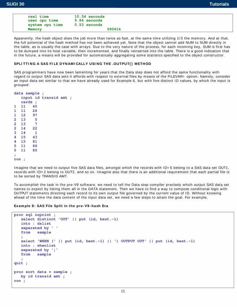
real time 10.54 seconds user cpu time 9.84 seconds system cpu time 0.53 seconds Memory 58061k Apparently, the hash object does the job more than twice as fast, at the same time utilizing 1/3 the memory. And at that, the full potential of the hash method has not been achieved yet. Note that the object cannot add NUM to SUM directly in the table, as is usually the case with arrays. Due to the very nature of the process, for each incoming key, SUM is first has to be dumped into its host variable, then incremented, and finally reinserted into the table. There is a good indication that in the future, a means will be provided for automatically aggregating some statistics specified to the object constructor. SPLITTING A SAS FILE DYNAMICALLY USING THE .OUTPUT() METHOD SAS programmers have now been lamenting for years that the Data step does not afford the same functionality with regard to output SAS data sets it affords with respect to external files by means of the FILEVAR= option. Namely, consider an input data set similar to that we have already used for Example 6, but with five distinct ID values, by which the input is grouped: data sample ; input id transid amt ; cards ; 1 11 40 1 11 26 1 12 97 2 13 5 2 13 7 2 14 22 3 14 1 4 15 43 4 15 81 5 11 86 5 11 85 ; run ; Imagine that we need to output five SAS data files, amongst which the records with ID=5 belong to a SAS data set OUT1, records with ID=2 belong to OUT2, and so on. Imagine also that there is an additional requirement that each partial file is to be sorted by TRANSID AMT. To accomplish the task in the pre-V9 software, we need to tell the Data step compiler precisely which output SAS data set names to expect by listing them all in the DATA statement. Then we have to find a way to compose conditional logic with OUTPUT statements directing each record to its own output file governed by the current value of ID. Without knowing ahead of the time the data content of the input data set, we need a few steps to attain the goal. For example, Example 8: SAS File Split in the pre-V9-hash Era proc sql noprint ; select distinct 'OUT' || put (id, best.-l) into : dslist separated by ' ' from sample ; select 'WHEN (' || put (id, best.-l) || ') OUTPUT OUT' || put (id, best.-l) into : whenlist separated by ';' from sample ; quit ; proc sort data = sample ; by id transid amt ; run ;

SUGI 30 Tutorials

16

data &dslist ; set sample ; select ( id ) ; &whenlist ; otherwise ; end ; run ; In Version 9, not only the hash object is instantiated at the run-time, but its method are also are run-time executables. Besides, the parameters passed to the object do not have to be constants, but they can be SAS variables. Thus, at any point at run-time, we can use the .OUTPUT() method to dump the contents of an entire hash table into a SAS data set, whose very name is formed using the SAS variable we need, and write the file out in one fell swoop: Example 9: SAS File Split Using the Hash .OUTPUT() Method data _null_ ; dcl hash hid (ordered: 'a') ; hid.definekey ('id', 'transid', 'amt', '_n_') ; hid.definedata ('id', 'transid', 'amt' ) ; hid.definedone ( ) ; do _n_ = 1 by 1 until ( last.id ) ; set sample ; by id ; hid.add() ; end ; hid.output (dataset: 'OUT' || put (id, best.-l)) ; run ; Above, the purpose of including _N_ in the hash key list is to make the key unique under any circumstances and thus output all records, even if they contain duplicates by TRANSID AMT. If such duplicates are to be deleted, we only need to kill the _N_ reference in the HID.DEFINEKEY() method. This step produces the following SAS log notes: NOTE: The data set WORK.OUT1 has 3 observations and 3 variables. NOTE: The data set WORK.OUT2 has 3 observations and 3 variables. NOTE: The data set WORK.OUT3 has 1 observations and 3 variables. NOTE: The data set WORK.OUT4 has 2 observations and 3 variables. NOTE: The data set WORK.OUT5 has 2 observations and 3 variables. NOTE: There were 11 observations read from the data set WORK.SAMPLE. To the eye of an alert reader knowing his Data step, but having not yet gotten his feet wet with the hash object in Version 9, the step above must look like a heresy. Indeed, how in the world is it possible to produce a SAS data set, let alone many, in a Data _Null_ step? It is possible because, with the hash object, the output is handled completely by and inside the object when the .OUTPUT() method is called, the Data step merely serving as a shell and providing parameter values to the object constructor. The step works as follows. Before the first record in each BY-group by ID is read, program control encounters the hash table declaration. It can be executed successfully because the compiler has provided the host variables for the keys and data. Then the DoW-loop reads the next BY-group one record at a time and uses its variables and _N_ to populate the hash table. Thus, when the DoW-loop is finished, the hash table for this BY-group is fully populated. Now control moves to the HID.OUTPUT() method. Its DATASET: parameter is passed the current ID value, which is concatenated with the character literal OUT. The method executes writing all the variables defined within the DefineKey() method from the hash table to the file with the name corresponding to the current ID. The Data step implied loop moves program control to the top of the step where it encounters the hash declaration. The old table is wiped out and a fresh empty table is instantiated. Then either the next BY-group starts, and the process is repeated, or the last record in the file has already been read, and the step stops after the SET statement hits the empty buffer. A PEEK AHEAD: HASHES OF HASHES In the Q&A part after our talk at SUGI 29, one of us (P.D.) was asked whether it was possible to create a hash table containing references to other hash tables in its entries. Having forgotten to judge not rashly, he answered “no” - and was wrong! Shortly after the Conference, Richard DeVenezia demonstrated in a post to the SAS-L list server that such construct is in fact possible, and, moreover, it can be quite useful practically. Since Richard published rather sophisticated examples of such usage on his web site, inquiring minds can point their browsers to

SUGI 30 Tutorials

17

http://www.devenezia.com/downloads/sas/samples/hash-6.sas Since after all, this is a tutorial, here we will discuss the technique a little closer to ab ovo.

xample 9 above, with the notable difference that it is not pre-grouped by ID. Say, it oks as follows:

ely, we need to output a SAS data set OUT1 containing all the records with ID=1, OUT2 – having

ulated from a whole single BY-group, umped out, destroyed, and re-created empty before the next BY-group commenced processing. However, in the case at

for all discrete ID values, and, as we go through e file, populate each table according to the ID value in the current record, and finally dump the table into corresponding

. How to address each of these tables programmatically using variable ID as a key?

idly so far, can no longer be used, for now we need to make HH a sort of a variable and be able to reference it accordingly. Luckily, the combined declaration above can be split

; ered: 'a') ;

object, whilst the _NEW_ method creates a new instance of it every time it owing excerpt:

rdered: 'a') ;

SAS File Split Problem Redefined Let us imagine an input file as in the elo data sample ; input id transid amt ; cards ; 5 11 86 2 14 22 1 12 97 3 14 1 4 15 43 2 13 5 2 13 7 1 11 40 4 15 81 5 11 85 1 11 26 ; run ;

problem has to be solved in a single Data step, without sorting or grouping the file beforehand in any Now and the same ay, shape, or form. Namw

all the records with ID=2 and so on, just as we did before. How can we do that? When the file was grouped by ID, it was easy because the hash table could be popdhand, we cannot follow the same path since pre-grouping is disallowed. Apparently, we should find a way to somehow keep separate hash tables thoutput files once end of file is reached. Two big questions on the path to the solution, are: 1. How to tell SAS 'create an aggregate collection of hash tables keyed by variable ID'? 2 Apparently, the method of declaring and instantiating a hash object all at once, i.e. dcl hash hh (ordered: 'a') ; < key/data definitions > hh.definedone () ;

s splendwhich has been serving uther than a sort of a literalra

into two phases: dcl hash hh ()hh = _new_ hash (ord This way, the DCL statement only declares the

executed at the run time. This, of course, means that the follisdcl hash hh () ; do i = 1 to 3 ; hh = _new_ hash (oend ;

SUGI 30 Tutorials

18

creates three instances of the object HH, that is, three separate hash tables. It leads us to the question #2 above, or, in other words, to the question: How to tell these tables apart? The first, crude, attempt, to arrive at a plausible answer would be to try displaying the values of HH with the PUT statement: 26 data _null_ ; 27 dcl hash hh () ; 28 do i = 1 to 3 ; 29 hh = _new_ hash (ordered: 'a') ; 30 put hh= ; ERROR: Invalid operation for object type. 31 end ; 32 run ; Obviously, even though HH looks like a ordinary Data step variable, it certainly is not. This is further confirmed by an attempt to store it in an array: 33 data _null_ ; 34 array ahh [3] ; 35 dcl hash hh () ; 36 do i = 1 to 3 ; 37 hh = _new_ hash (ordered: 'a') ; 38 ahh [i] = hh ; ERROR: Object of type hash cannot be converted to scalar. 39 end ; 40 run ; So, we cannot store the collection of "values" HH assumes anywhere in a regular Data step structure. Then, where can we store it? In another hash table, of course! In a hash table, "data" can mean numeric or character Data step variables, but it also can mean an object. Getting back to the current problem, the new "hash of hashes" table, let us call it, say, HOH, will contain the hashes pertaining to different ID values as its data portion. The only other component we need to render HOH fully operative is a key. Since we need to identify different hash tables by ID, this is the key variable we are looking for. Finally, in order to go through the hash table of hashes and select them for output one by one, we need to give the HOH table an iterator, which below will be called HIH. Now we can easily put it all together: Example 10: Spliting an Unsorted SAS File a Hash of Hashes and the .OUTPUT() Method data sample ; input id transid amt ; cards ; 5 11 86 2 14 22 1 12 97 3 14 1 4 15 43 2 13 5 2 13 7 1 11 40 4 15 81 5 11 85 1 11 26 ; run ; data _null_ ; dcl hash hoh (ordered: 'a') ; dcl hiter hih ('hoh' ) ; hoh.definekey ('id' ) ; hoh.definedata ('id', 'hh' ) ; hoh.definedone () ; dcl hash hh () ; do _n_ = 1 by 1 until ( eof ) ;

SUGI 30 Tutorials

19

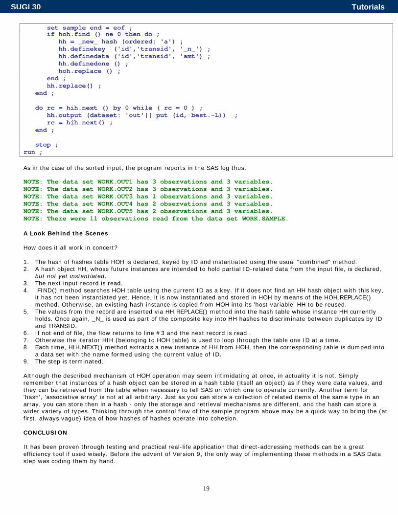
set sample end = eof ; if hoh.find () ne 0 then do ; hh = _new_ hash (ordered: 'a') ; hh.definekey ('id','transid', '_n_') ; hh.definedata ('id','transid', 'amt') ; hh.definedone () ; hoh.replace () ; end ; hh.replace() ; end ; do rc = hih.next () by 0 while ( rc = 0 ) ; hh.output (dataset: 'out'|| put (id, best.-L)) ; rc = hih.next() ; end ; stop ; run ; As in the case of the sorted input, the program reports in the SAS log thus: NOTE: The data set WORK.OUT1 has 3 observations and 3 variables. NOTE: The data set WORK.OUT2 has 3 observations and 3 variables. NOTE: The data set WORK.OUT3 has 1 observations and 3 variables. NOTE: The data set WORK.OUT4 has 2 observations and 3 variables. NOTE: The data set WORK.OUT5 has 2 observations and 3 variables. NOTE: There were 11 observations read from the data set WORK.SAMPLE. A Look Behind the Scenes How does it all work in concert? 1. The hash of hashes table HOH is declared, keyed by ID and instantiated using the usual "combined" method. 2. A hash object HH, whose future instances are intended to hold partial ID-related data from the input file, is declared,

but not yet instantiated. 3. The next input record is read. 4. .FIND() method searches HOH table using the current ID as a key. If it does not find an HH hash object with this key,

it has not been instantiated yet. Hence, it is now instantiated and stored in HOH by means of the HOH.REPLACE() method. Otherwise, an existing hash instance is copied from HOH into its 'host variable' HH to be reused.

5. The values from the record are inserted via HH.REPLACE() method into the hash table whose instance HH currently holds. Once again, _N_ is used as part of the composite key into HH hashes to discriminate between duplicates by ID and TRANSID.

6. If not end of file, the flow returns to line #3 and the next record is read . 7. Otherwise the iterator HIH (belonging to HOH table) is used to loop through the table one ID at a time. 8. Each time, HIH.NEXT() method extracts a new instance of HH from HOH, then the corresponding table is dumped into

a data set with the name formed using the current value of ID. 9. The step is terminated. Although the described mechanism of HOH operation may seem intimidating at once, in actuality it is not. Simply remember that instances of a hash object can be stored in a hash table (itself an object) as if they were data values, and they can be retrieved from the table when necessary to tell SAS on which one to operate currently. Another term for 'hash', 'associative array' is not at all arbitrary. Just as you can store a collection of related items of the same type in an array, you can store then in a hash - only the storage and retrieval mechanisms are different, and the hash can store a wider variety of types. Thinking through the control flow of the sample program above may be a quick way to bring the (at first, always vague) idea of how hashes of hashes operate into cohesion. CONCLUSION It has been proven through testing and practical real-life application that direct-addressing methods can be a great efficiency tool if used wisely. Before the advent of Version 9, the only way of implementing these methods in a SAS Data step was coding them by hand.

SUGI 30 Tutorials

20

The Data step hash object provides an access to algorithms of the same type and hence with the same high-performance potential via a canned routine. It makes it unnecessary for a programmer to know the details, for great results - on par or better than hand-coding - can be achieved just by following syntax rules and learning which methods cause the hash object to produce the coveted results. Thus, along with improving computer efficiency, the Data step hash objects also makes better programming efficiency. Finally, it should be noted that at this moment of the Version 9 history, the hash object and its methods have matured enough to come out of the experimental stage. To the extent of our testing, they do work as documented. From the programmer’s viewpoint, some aspects that might need attention are: • Parameter type matching in the case where a table is loaded from a data set. If the data set is named in the step, the

attributes of hash entries should be available from its descriptor. • The need to define the key variable additionally as a data element in order to extract the key from the table still looks

a bit awkward. • If the name of a dataset is provided to the constructor, a SAS programmer naturally expects its attributes to be

available at the compile time. Currently, the compiler cannot see inside the parentheses of the hash declaration. Perhaps the ability to parse the content would be a useful feature to be addressed in the future.

Putting it all aside, the advent of the production Data step hash objects as the first dynamic Data step structure is nothing short of a long-time breakthrough. This novel structure allows a SAS Data step programmer to do the following, just to name a few: • Create, at the Data step run-time, a memory-resident table which keyed by practically any composite key. • Search for keys in, retrieve entries from, add entries into, replace entries in, remove entries from, the table - all in

practically O(1), i.e. constant, time. • Create a hash iterator object for a table allowing to access the table entries sequentially. • Delete both the hash table and its iterator at the run-time as needed. • Make the table internally ordered automatically by a given key, as entries are added/replaced. • Load the table from a SAS file via the DATASET parameter without explicit looping. • Unload the table sequentially key by key using the iterator object declared for the table. • Create, at the run-time, a single (or multiple) binary search AVL tree, whose memory is allocated/released dynamically

as the tree is grown or shrunk. • Use the hash table as a quickly searchable lookup table to facilitate file matching process without the need to sort and

merge. • Use the internal order of the hash table to rapidly sort large arrays of any type, including temporary. • Dump the content of a hash table to a SAS data file in one fell swoop using the .OUTPUT() method. • Create the names of the files to be dumped depending on a SAS variable on the fly - the new functionality similar to

that of the FILEVAR= option on the FILE statement. • Use this functionality to “extrude” input through hash object(s) to split it in a number of SAS files with SAS-variable-

governed names - if necessary, internally ordered. • Use a hash table to store and search references to other hash tables in order to process them conditionally. • Use hash table objects to organize true run-time Data step dynamic dictionaries. • Use such dictionaries to speed up the calculation of simple statistics instead of MEANS/SUMMARY procedures, when the

latter choke on a high cardinality of their classification variables. SAS is a registered trademark or trademark of SAS Institute, Inc. in the USA and other countries. ® indicates USA registration. REFERENCES P.Dorfman. Table Lookup by Direct Addressing: Key-Indexing, Bitmapping, Hashing. SUGI 26, Long Beach, CA, 2001. P.Dorfman, G.Snell. Hashing Rehashed. SUGI 27, Orlando, FL, 2002. D.E.Knuth. The Art of Computer Programming, 3. T.Standish. Data Structures, Algorithms & Software Principles in C. J.Secosky. The Data step in Version 9: What’s New? SUGI 27, Orlando, FL, 2002. P.Dorfman, G.Snell. Hashing: Generations. SUGI 28, Seattle, WA, 2003. P.Dorfman, K.Vyverman. Hash Component Objects: Dynamic Data Storage and Table Look-Up. SUGI 29, Montreal, 2004. P.Dorfman, L.Shajenko. Data Step Programming Using the Hash Objects, NESUG 2004, Baltimore, MD 2004. AUTHOR CONTACT INFORMATION Paul M. Dorfman Koen Vyverman4437 Summer Walk Ct., Frevolaan 69 Jacksonville, FL 32258 SAS Institute B.V.

SUGI 30 Tutorials

21

(904) 260-6509 Huizen, Netherlands 1270 (904) 226-0743 011-31-20-773-9606 sashole@bellsouth.net goldbluff@mac.com

SUGI 30 Tutorials