230B: Public Economics

Capital Taxation

Emmanuel Saez

Berkeley

1

MOTIVATION

1) Capital income is about 25% of national income (labor

income is 75%) but distribution of capital income is much

more unequal than labor income

Capital income inequality is due to differences in savings be-

havior but also inheritances received

⇒ Equity suggests it should be taxed more than labor

2) Capital Accumulation correlated strongly with growth [al-

though causality link is not obvious] and capital accumulation

might be sensitive to the net-of-tax return.

⇒ Efficiency cost of capital taxation might be high.

2

MOTIVATION

3) Capital more mobile internationally than labor

Key distinction is residence vs. source base capital taxation:

Residence: Capital income tax based on residence of owner

of capital.

Most individual income tax systems are residence based (with

credits for taxes paid abroad)

Incidence falls on owner⇒ can only escape tax through evasion

(tax heavens) or changing residence (mobility of persons)

Tax evasion of capital income through tax heavens is a very

serious concern (Zucman QJE’13, ’15)

3

Source: Capital income tax based on location of capital (mostcorporate income tax systems are source based)

Incidence is then partly shifted to labor if capital is mobile.

Example: Open economy with fully mobile capital and sourcetaxation: Local GDP: wL + rK = F (K,L) = L · F (K/L,1) =L · f(k) where k = K/L is capital stock per worker

Net-of-tax rate of return is fixed by the international rate ofreturn r∗ so that (1 − τc)FK(K,L) = (1 − τc)f ′(k) = r∗ wherek = K/L is capital stock per worker and τc corp tax rate

As wL+r∗K = F (K,L), wage w = FL(K,L) = f(k)−r∗ ·k fallswith τc

4) Capital taxation is extremely complex and provides manytax avoidance opportunities

MACRO FRAMEWORK

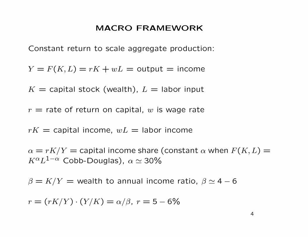
Constant return to scale aggregate production:

Y = F (K,L) = rK + wL = output = income

K = capital stock (wealth), L = labor input

r = rate of return on capital, w is wage rate

rK = capital income, wL = labor income

α = rK/Y = capital income share (constant α when F (K,L) =KαL1−α Cobb-Douglas), α ' 30%

β = K/Y = wealth to annual income ratio, β ' 4− 6

r = (rK/Y ) · (Y/K) = α/β, r = 5− 6%

4

0%

100%

200%

300%

400%

500%

600%

700%

800%

UK France US South US North

% n

atio

nal i

ncom

e

Figure 11: National wealth in 1770-1810: Old vs. New world

Other domestic capital

Housing

Slaves

Agricultural Land

10%

15%

20%

25%

30%

35%

40%

1975 1980 1985 1990 1995 2000 2005 2010

Figure 12: Capital shares in factor-price national income 1975-2010

USA Japan Germany France UK Canada Australia Italy

43

Source: Piketty and Zucman (2014)

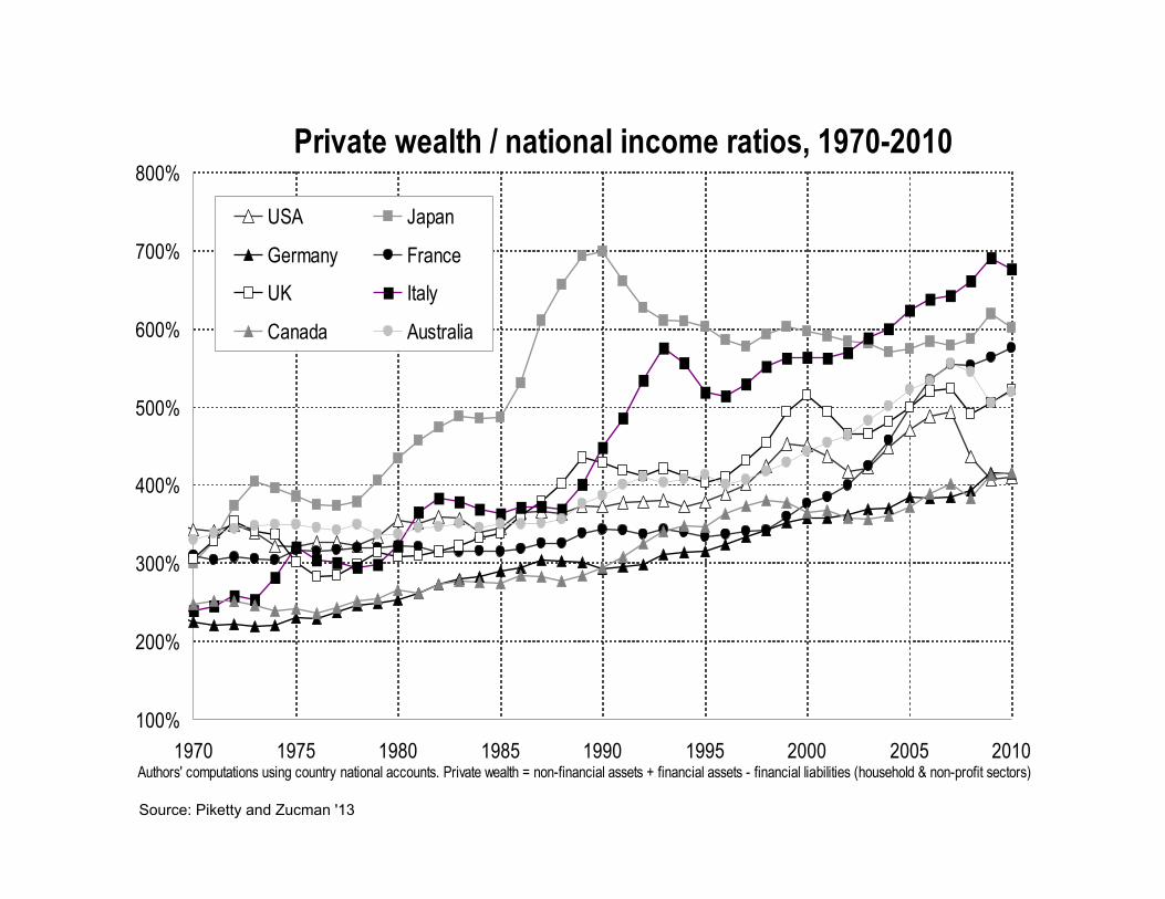
Private wealth / national income ratios, 1970-2010

100%

200%

300%

400%

500%

600%

700%

800%

1970 1975 1980 1985 1990 1995 2000 2005 2010Authors' computations using country national accounts. Private wealth = non-financial assets + financial assets - financial liabilities (household & non-profit sectors)

USA Japan

Germany France

UK Italy

Canada Australia

Source: Piketty and Zucman '13

Private wealth / national income ratios 1870-2010

100%

200%

300%

400%

500%

600%

700%

800%

1870 1890 1910 1930 1950 1970 1990 2010Authors' computations using country national accounts. Private wealth = non-financial assets + financial assets - financial liabilities (household & non-profit sectors)

USA

Europe

Source: Piketty and Zucman '13

The changing nature of national wealth, UK 1700-2010

0%

100%

200%

300%

400%

500%

600%

700%

800%

1700 1750 1810 1850 1880 1910 1920 1950 1970 1990 2010National wealth = agricultural land + housing + other domestic capital goods + net foreign assets

(% n

atio

nal i

ncom

e)

Net foreign assets

Other domestic capital

Housing

Agricultural land

Source: Piketty, Handbook chapter, 2014

The changing nature of national wealth, France 1700-2010

0%

100%

200%

300%

400%

500%

600%

700%

800%

1700 1750 1780 1810 1850 1880 1910 1920 1950 1970 1990 2010National wealth = agricultural land + housing + other domestic capital goods + net foreign assets

(% n

atio

nal i

ncom

e)

Net foreign assets

Other domestic capital

Housing

Agricultural land

Source: Piketty, Handbook chapter, 2014

The changing nature of national wealth, US 1770-2010 (incl. slaves)

0%

100%

200%

300%

400%

500%

600%

1770 1810 1850 1880 1910 1920 1930 1950 1970 1990 2010

National wealth = agricultural land + housing + other domestic capital goods + net foreign assets

(% n

atio

nal i

ncom

e)

Net foreign assetsOther domestic capitalHousingSlavesAgricultural land

Source: Piketty and Zucman '13

Piketty (2014) book: Capital in the 21st Century

Analyzes income, wealth, inheritance data over the long-run:

1) Growth rate n+g = population growth + growth per capita.

Population growth will converge to zero, growth per capita for

frontier economies is modest (1%)⇒ long-run g ' 1%, n ' 0%

2) Long-run steady-state Wealth to income ratio (β) = savings

rate (s) / annual growth (n+ g): β = s/(n+ g)

Proof: Kt+1 = (1+n+g) ·Kt = Kt+s ·Yt ⇒ Kt/Yt = s/(n+g)

With s = 8% and n + g = 2%, β = 400% but with s = 8%

and n+ g = 1%, β = 800% ⇒ Wealth will become important

6

Piketty (2014) book: Capital in the 21st Century

3) After-tax rate of return on wealth r = r(1− τK) = 4− 5%

significantly larger than n + g [except exceptional period of

1930–1970]

With r > n + g, role of inheritance in wealth and wealth con-

centration become large [past swallows the future]

Explanation: Rentier who saves all his return on wealth ac-

cumulates wealth at rate r bigger than n + g and hence his

wealth grows relative to the size of the economy. The bigger

r − (n+ g), the easier it is for wealth to “snowball”

⇒ Capital taxation reduces r to r = r · (1 − τK) ⇒ This can

reduce wealth concentration

7

2%

3%

4%

5%

6%

Annu

al ra

te o

f ret

urn

or ra

te o

f gro

wth

Figure 10.10. After tax rate of return vs. growth rate at the world level, from Antiquity until 2100

Pure rate of return to capital (after tax and capital losses)

Growth rate of world output g

0%

1%

0-1000 1000-1500 1500-1700 1700-1820 1820-1913 1913-1950 1950-2012 2012-2050 2050-2100

Annu

al ra

te o

f ret

urn

or ra

te o

f gro

wth

The rate of return to capital (after tax and capital losses) fell below the growth rate during the 20th century, and may again surpass it in the 21st century. Sources and series : see piketty.pse.ens.fr/capital21c

Source: Piketty (2014)

WEALTH AND CAPITAL INCOME IN AGGREGATE

Definition: Capital Income = Returns from Wealth Holdings

Aggregate US Personal Wealth ' 4*GDP ' $60 Tr

Tangible assets: residential real estate (land+buildings) [in-come = rents] and unincorporated business + farm assets[income = profits]

Financial assets: corporate stock [income = dividends + re-tained earnings], fixed claim assets (corporate and govt bonds,bank accounts) [income = interest]

Liabilities: Mortgage debt, Student loans, Consumer creditdebt

Substantial amount of financial wealth is held indirectly through:pension funds [DB+DC], mutual funds, insurance reserves

9

0%

100%

200%

300%

400%

500%

1913

1918

1923

1928

1933

1938

1943

1948

1953

1958

1963

1968

1973

1978

1983

1988

1993

1998

2003

2008

2013

% o

f nat

iona

l inc

ome

The composition of household wealth in the U.S., 1913-2013

Housing (net of mortgages)

Sole proprietorships & partnerships

Currency, deposits and bonds Equities

Pensions

Source: Saez and Zucman (2014)

0%

5%

10%

15%

20%

25%

30%

35% 19

13

1918

1923

1928

1933

1938

1943

1948

1953

1958

1963

1968

1973

1978

1983

1988

1993

1998

2003

2008

2013

% o

f fac

tor-

pric

e na

tiona

l inc

ome

The composition of capital income in the U.S., 1913-2013

Housing rents (net of mortgages)

Noncorporate business profits

Net interest Corporate profits

Profits & interest paid to pensions

Source: Saez and Zucman (2014)

INDIVIDUAL WEALTH AND CAPITAL INCOME

Wealth = W , Return = r, Capital Income = rW

Wt = Wt−1 + rtWt−1 + Et + It − Ct

where Wt is wealth at age t, Ct is consumption, Et labor in-

come earnings (net of taxes), rt is the average (net) rate of

return on investments and It net inheritances (gifts received

and bequests minus gifts given).

Replacing Wt−1 and so on, we obtain the following expression

(assuming initial wealth W0 is zero):

Wt =t∑

k=1

(Ek − Ck + Ik)t∏

j=k+1

(1 + rj)

11

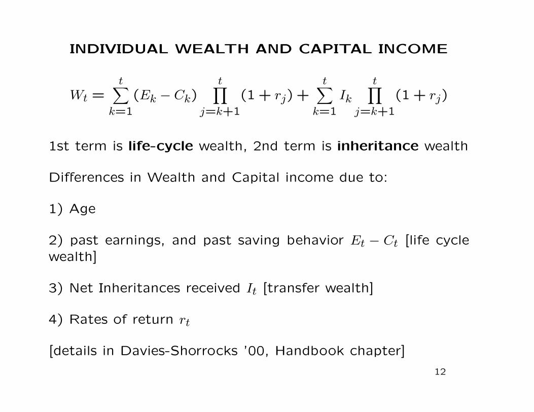
INDIVIDUAL WEALTH AND CAPITAL INCOME

Wt =t∑

k=1

(Ek − Ck)t∏

j=k+1

(1 + rj) +t∑

k=1

Ik

t∏j=k+1

(1 + rj)

1st term is life-cycle wealth, 2nd term is inheritance wealth

Differences in Wealth and Capital income due to:

1) Age

2) past earnings, and past saving behavior Et − Ct [life cyclewealth]

3) Net Inheritances received It [transfer wealth]

4) Rates of return rt

[details in Davies-Shorrocks ’00, Handbook chapter]

12

WEALTH DISTRIBUTION

Wealth inequality is very large (much larger than labor income)

US Household Wealth is divided 1/3,1/3,1/3 for the top 1%,the next 9%, and the bottom 90% [bottom 1/2 householdshold almost no wealth]

Financial wealth is more unequally distributed than (net) realestate wealth

Share of real estate wealth falls at the top of the wealth dis-tribution

Growth of private pensions [such as 401(k) plans] has “de-mocratized” stock ownership in the US

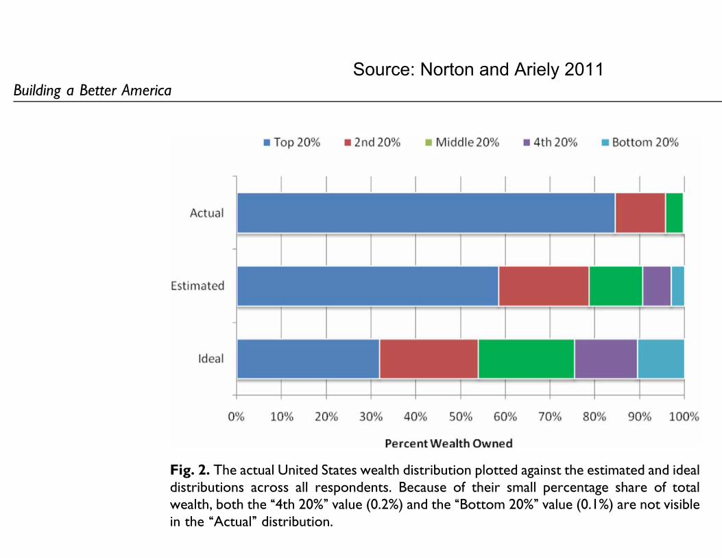
US public underestimates extent of wealth inequality and thinksthe ideal wealth distribution should be a lot less unequal [Norton-Ariely ’11]

13

agreed that such redistribution should take the form of moving

wealth from the top quintile to the bottom three quintiles. In

short, although Americans tend to be relatively more

favorable toward economic inequality than members of other

countries (Osberg & Smeeding, 2006), Americans’ consensus

about the ideal distribution of wealth within the United States

Fig. 3. The actual United States wealth distribution plotted against the estimated and idealdistributions of respondents of different income levels, political affiliations, and genders.Because of their small percentage share of total wealth, both the ‘‘4th 20%’’ value (0.2%)and the ‘‘Bottom 20%’’ value (0.1%) are not visible in the ‘‘Actual’’ distribution.

Fig. 2. The actual United States wealth distribution plotted against the estimated and idealdistributions across all respondents. Because of their small percentage share of totalwealth, both the ‘‘4th 20%’’ value (0.2%) and the ‘‘Bottom 20%’’ value (0.1%) are not visiblein the ‘‘Actual’’ distribution.

Building a Better America 11

at Harvard Libraries on February 3, 2011pps.sagepub.comDownloaded from

Source: Norton and Ariely 2011

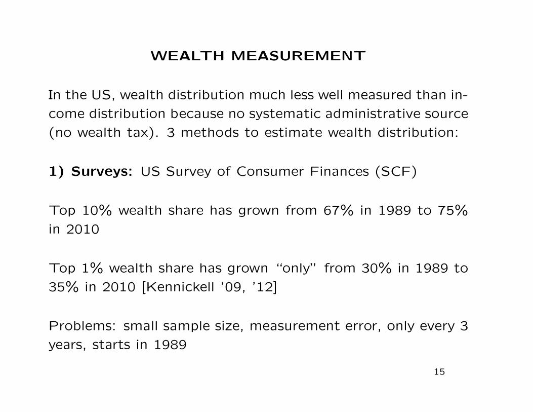
WEALTH MEASUREMENT

In the US, wealth distribution much less well measured than in-

come distribution because no systematic administrative source

(no wealth tax). 3 methods to estimate wealth distribution:

1) Surveys: US Survey of Consumer Finances (SCF)

Top 10% wealth share has grown from 67% in 1989 to 75%

in 2010

Top 1% wealth share has grown “only” from 30% in 1989 to

35% in 2010 [Kennickell ’09, ’12]

Problems: small sample size, measurement error, only every 3

years, starts in 1989

15

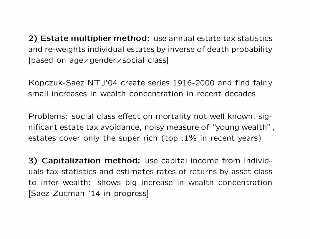
2) Estate multiplier method: use annual estate tax statistics

and re-weights individual estates by inverse of death probability

[based on age×gender×social class]

Kopczuk-Saez NTJ’04 create series 1916-2000 and find fairly

small increases in wealth concentration in recent decades

Problems: social class effect on mortality not well known, sig-

nificant estate tax avoidance, noisy measure of “young wealth”,

estates cover only the super rich (top .1% in recent years)

3) Capitalization method: use capital income from individ-

uals tax statistics and estimates rates of returns by asset class

to infer wealth: shows big increase in wealth concentration

[Saez-Zucman ’14 in progress]

50%  

55%  

60%  

65%  

70%  

75%  

80%  

85%  

90%  1913  

1918  

1923  

1928  

1933  

1938  

1943  

1948  

1953  

1958  

1963  

1968  

1973  

1978  

1983  

1988  

1993  

1998  

2003  

2008  

Top  10%  Wealth  Shares:  Comparing  Es8mates  

Capitalized  Incomes  (Saez-­‐Zucman)  

SCF  (Kennickell)  

0%  

5%  

10%  

15%  

20%  

25%  

30%  

35%  

40%  

45%  

50%  1913  

1918  

1923  

1928  

1933  

1938  

1943  

1948  

1953  

1958  

1963  

1968  

1973  

1978  

1983  

1988  

1993  

1998  

2003  

2008  

Top  1%  Wealth  Shares:  Comparing  Es7mates  

Capitalized  Incomes  (Saez-­‐Zucman)  

Estates  (Kopczuk-­‐Saez  and  IRS)  

SCF  (Kennickell)  

Source: Saez and Zucman (2014)

0%

5%

10%

15%

20%

25%

30% 19

13

1918

1923

1928

1933

1938

1943

1948

1953

1958

1963

1968

1973

1978

1983

1988

1993

1998

2003

2008

2013

Top 0.1% wealth share in the U.S., 1913-2012

0%

2%

4%

6%

8%

10%

12%

14%

1960 1965 1970 1975 1980 1985 1990 1995 2000 2005 2010 2015

Top wealth shares: decomposing the top 1%

Top 0.01%

Top 0.1%-0.01%

Top 0.5%-0.1%

Top 1%-0.5%

0%

5%

10%

15%

20%

25%

30%

35%

40%

45% 19

17

1922

1927

1932

1937

1942

1947

1952

1957

1962

1967

1972

1977

1982

1987

1992

1997

2002

2007

2012

% o

f net

hou

seho

ld w

ealth

Composition of the bottom 90% wealth share

Pensions

Business assets

Housing (net of mortgages)

Equities & fixed claims (net of non-mortgage debt)

Source: Saez and Zucman (2014)

0%

10%

20%

30%

40%

50%

60%

70%

80%

90%

100%

1810 1830 1850 1870 1890 1910 1930 1950 1970 1990 2010

Sha

re o

f top

dec

ile o

r per

cent

ile in

tota

l wea

lth

The top 10% wealth holders own about 80% of total wealth in 1929, and 75% today.

Figure 3.5. Wealth inequality in the U.S., 1810-2010

Top 10% wealth chare

Top 1% wealth share

0%

10%

20%

30%

40%

50%

60%

70%

80%

90%

100%

1810 1830 1850 1870 1890 1910 1930 1950 1970 1990 2010

Sha

re o

f top

dec

ile o

r per

cent

ile in

tota

l wea

lth

The top decile (the top 10% highest wealth holders) owns 80-90% of total wealth in 1810-1910, and 60-65% today.

Figure 3.1. Wealth inequality in France, 1810-2010

Top 10% wealth share

Top 1% wealth share

Source: Piketty and Zucman '14, handbook chapter

0%

10%

20%

30%

40%

50%

60%

70%

80%

90%

100%

1810 1830 1850 1870 1890 1910 1930 1950 1970 1990 2010

Sha

re o

f top

dec

ie o

r top

per

cent

ile in

tota

l wea

lth

The top decile owns 80-90% of total wealth in 1810-1910, and 70% today.

Figure 3.3. Wealth inequality in the United Kingom, 1810-2010

Top 10% wealth share

Top 1% wealth share

Source: Piketty and Zucman '14, handbook chapter

0%

10%

20%

30%

40%

50%

60%

70%

80%

90%

100%

1810 1830 1850 1870 1890 1910 1930 1950 1970 1990 2010

Sha

re o

f top

dec

ie o

r per

cent

ile in

tota

l wea

lth

The top 10% holds 80-90% of total wealth in 1810-1910, and 55-60% today.

Figure 3.4. Wealth inequality in Sweden, 1810-2010

Top 10% wealth share

Top 1% wealth share

Source: Piketty and Zucman '14, handbook chapter

CAPITAL TAXATION IN THE US

Good US references: Gravelle ’94 book, Slemrod-Bakija ’04book

1) Corporate Income Tax (fed+state): 35% Federal taxrate on profits of corporations [complex rules with many in-dustry specific provisions]: effective tax rate much lower andincidence depends on mobility of capital

2) Individual Income Tax (fed+state): taxes many forms ofcapital income

Realized capital gains and dividends (dividends since ’03 only)receive preferential treatment

Imputed rent of home owners, returns on pension funds, state+localgovernment bonds interest are exempt

19

FACTS OF US CAPITAL INCOME TAXATION

3) Estate and gift taxes:

Fed taxes estates above $5.5M exemption (only .1% of de-ceased liable), tax rate is 40% above exemption (2013+)

Charitable and spousal giving is exempt

Substantial tax avoidance activity through tax accountants

Step-up of realized capital gains at death (lock-in effect)

4) Property taxes (local) on real estate (old tax):

Tax varies across jurisdictions. About 0.5% of market valueon average, like a 10% tax on imputed rent if return is 5%

Lock-in effect in states that use purchase price base such asCalifornia

20

LIFE CYCLE VS. INHERITED WEALTH

Old view: Tobin and Modigliani: life cycle wealth accountsfor the bulk of the wealth held in the US. Kotlikoff-SummersJPE’81 challenged the old view (debate Kotlikoff vs. Modiglianiin JEP’88)

Why is this question important?

1) Economic Modeling: what accounts for wealth accumula-tion and inequality? Is widely used life-cycle model with nobequests a good approximation?

2) Policy Implications: taxation of capital income and estates.Role of pay-as-you-go vs. funded retirement programs

Key problem is that the definition of life-cycle vs. inheritedwealth is not conceptually clean (Modigliani does not capitalizeinherited wealth while Kotlikoff-Summers do)

21

LIFE CYCLE VS. INHERITED WEALTH

Piketty-Postel-Vinay-Rosenthal EEH’14 (PPVR) propose bet-

ter definition to resolve Modigliani vs. Kotlikoff-Summers con-

troversy (see Piketty-Zucman Handbook chapter ’14)

Individual wealth accumulation:

Wt =t∑

k=1

(Ek − Ck) · (1 + r)t−k +t∑

k=1

Ik · (1 + r)t−k

If Wt >∑t

k=1 Ik · (1 + r)t−k then individual also saves out of labor income

Ek and inherited wealth is∑t

k=1 Ik · (1 + r)t−k

If Wt ≤∑t

k=1 Ik · (1 + r)t−k then individual consumes part of inheritances(in addition to labor income) and inherited wealth is Wt

PPVR requires micro-data for implementation. If we assume uniformsaving rate s, there is a simplified formula for share of inherited wealthby/[by+(1−α) ·s] with by bequest flow/national income and α capital share

22

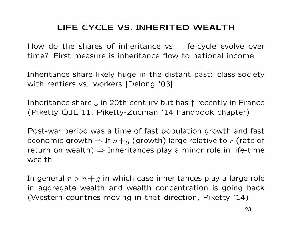
LIFE CYCLE VS. INHERITED WEALTH

How do the shares of inheritance vs. life-cycle evolve overtime? First measure is inheritance flow to national income

Inheritance share likely huge in the distant past: class societywith rentiers vs. workers [Delong ’03]

Inheritance share ↓ in 20th century but has ↑ recently in France(Piketty QJE’11, Piketty-Zucman ’14 handbook chapter)

Post-war period was a time of fast population growth and fasteconomic growth⇒ If n+g (growth) large relative to r (rate ofreturn on wealth) ⇒ Inheritances play a minor role in life-timewealth

In general r > n+g in which case inheritances play a large rolein aggregate wealth and wealth concentration is going back(Western countries moving in that direction, Piketty ’14)

23

LONG-RUN EVOLUTION OF INHERITANCE 1073

FIGURE IAnnual Inheritance Flow as a Fraction of National Income, France, 1820–2008

accordingtoourlatest data point (2008), it is nowcloseto15% (seeFigure I).

Ifwetakealongerrunperspective, thenthetwentieth-centuryU-shaped pattern looks even more spectacular. The inheritanceflow was relatively stable around 20–25% of national incomethroughout the 1820–1910 period (with a slight upward trend),before being divided by a factor of about 5–6 between 1910 andthe 1950s, and then multiplied by a factor of about 3–4 betweenthe 1950s and the 2000s.

These are truly enormous historical variations, but theyappear tobe well founded empirically. In particular, we find simi-larpatterns withourtwofullyindependent estimates of theinher-itance flow. The gap between our “economic flow” (computed fromnational wealth estimates, mortality tables, and observed age-wealth profiles) and “fiscal flow” series (computed from bequestand gift tax data) can be interpreted as a measure of tax eva-sion and other measurement errors. This gap appears to approx-imately constant over time and relatively small, so that our twoseries deliver fairly consistent long-run patterns (see Figure I).

If we use disposable income (national income minus taxesplus cash transfers) rather than national income as the denomi-nator, then we findthat the inheritance flowobservedin the earlytwenty-first century is back to about 20%, that is, approximatelythe same level as that observed one century ago. This comes fromthe fact that disposable income was as high as 90–95% of national

at University of C

alifornia, Berkeley on January 19, 2012

http://qje.oxfordjournals.org/D

ownloaded from

Source: Piketty QJE'11

0%

4%

8%

12%

16%

20%

24%

1900 1910 1920 1930 1940 1950 1960 1970 1980 1990 2000 2010

Annu

al flo

w of

bequ

ests

and g

ifts (%

nati

onal

incom

e)

The inheritance flow follows a U-shaped in curve in France as well as in the U.K. and Germany. It is possible that gifts are under-estimated in the U.K. at the end of the period.

Figure 4.5. The inheritance flow in Europe 1900-2010

France

U.K.

Germany

Source: Piketty and Zucman '14, handbook chapter

20%

30%

40%

50%

60%

70%

80%

90%

100%

1850 1870 1890 1910 1930 1950 1970 1990 2010

Cumu

lated

stoc

k of in

herite

d wea

lth (%

priv

ate w

ealth

)

Inherited wealth represents 80-90% of total wealth in France in the 19th century; this share fell to 40%-50% during the 20th century, and is back to about 60-70% in the early 21st century.

Figure 4.4. The cumulated stock of inherited wealth as a fraction of aggregate private wealth, France 1850-2010

Share of inherited wealth (PPVR definition, extrapolation)

Share of inherited wealth (simplified definition, lower bound)

Source: Piketty and Zucman '14, handbook chapter

20%

30%

40%

50%

60%

70%

80%

90%

100%

1900 1910 1920 1930 1940 1950 1960 1970 1980 1990 2000 2010

Stoc

k of in

herite

d we

alth(

% p

rivate

wea

lth)

The inheritance share in aggregate wealth accumulation follows a U-shaped curve in France and Germany (and to a more limited extent in the U.K. and Germany. It is possible that gifts are under-estimated in the U.K. at the end of the period.

Figure 4.6. The inheritance stock in Europe 1900-2010 (simplified definitions using inheritance vs. saving flows) (approximate, lower-bound estimates)

France

U.K.

Germany

Source: Piketty and Zucman '14, handbook chapter

TAXES IN OLG LIFE-CYCLE MODEL

max U = u(c1, l1) + δu(c2, l2)

No tax situation: earn w1l1 in period 1, w2l2 in period 2

Savings s = w1l1 − c1, c2 = w2l2 + (1 + r)s

Capital income rs

Intertemporal budget with no taxes:

c1 + c2/(1 + r) ≤ w1l1 + w2l2/(1 + r)

This model has uniform rate of return and does not capture

excess returns

25

TAXES IN OLG MODEL

Budget with consumption tax tc:

(1 + tc)[c1 + c2/(1 + r)] ≤ w1l1 + w2l2/(1 + r)

Budget with labor income tax τL:

c1 + c2/(1 + r) ≤ (1− τL)[w1l1 + w2l2/(1 + r)]

Consumption and labor income tax are equivalent if

1 + tc = 1/(1− τL)

Both taxes distort only labor-leisure choice

26

TAXES IN OLG MODEL

Budget with capital income tax τK:

c1 + c2/(1 + r(1− τK)) ≤ w1l1 + w2l1/(1 + r(1− τK))

τK distorts only inter-temporal consumption choice

Budget with comprehensive income tax τ :

c1 + c2/(1 + r(1− τ)) ≤ (1− τ)[w1l1 + w2l2/(1 + r(1− τ))]

τ distorts both labor-leisure and inter-temporal consumption

choices

τ imposes “double” tax: (1) tax on earnings, (2) tax on sav-

ings

27

EFFECT OF r ON SAVINGS

Assume that labor supply is fixed. Draw graph. Suppose r ↑:

1) Substitution effect: price of c2 ↓ ⇒ c2 ↑, c1 ↓ ⇒ savings

s = w1l1 − c1 ↑.

2) Wealth effect: Price of c2 ↓ ⇒ both c1 and c2 ↑ ⇒ save less

3) Human wealth effect: present discounted value of labor

income ↓ ⇒ both c1 and c2 ↓ ⇒ save more

Note: If w2l2 < c2 (ie s > 0), 2)+3) ⇒ save less

Total net effect is theoretically ambiguous ⇒ τK has ambigu-

ous effects on s

28

SHIFT FROM LABOR TO CONSUMPTION TAX

Labor and consumption are equivalent for the individual if 1 +tc = 1/(1− τL) but savings pattern is different

Assume w2 = 0 and l1 = 1

(1 + tc)[c1 + c2/(1 + r)] = w1 with consumption tax

c1 + c2/(1 + r) = (1− tL)w1 with labor tax

1) Consumption tax tc: cc1 = (w1 − sc)/(1 + tc), cc2 = (1 +r)sc/(1 + tc)

2) Labor income tax τL: cL1 = w1(1− τL)− sL, cL2 = (1 + r)sL

Same consumption in both cases so sL = sc/(1 + tc) ⇒ Savemore with a consumption tax

29

TRANSITION FROM LABOR TO C TAX

In OLG model and closed economy, capital stock is due to

life-cycle savings s

Start with labor tax τL and switch to a consumption tax tc

The old [at time of transition] would have paid nothing in

labor tax regime but now have to pay tax on c2

For the young [and future generations], the two regimes look

equivalent so they now save more and increase the capital

stock

However, this increase in capital stock comes at the price of

hurting the old who are taxed twice

30

TRANSITION FROM LABOR TO C TAX

Suppose the government keeps the old as well off as in previoussystem by exempting them from consumption tax

This creates a deficit in government budget equal to

d = τLw1 − tcc1 = tcw1/(1 + tc)− tcc1 = tcsL

Extra saving by the young is sc − sL = tcsL exactly equal togovernment deficit.

Full neutrality result: Extra savings of young is equal to oldcapital stock + new government deficit ⇒ no change in theaggregate capital stock

Full neutrality depends crucially on same r for govt debt andaggregate r [in practice: equity premium puzzle]

[Same result for Social Security privatization]

31

OPTIMAL CAPITAL INCOME TAXATION

Complex problem with many sub-literatures: Banks and Dia-

mond Mirrlees Review ’09 provide recent survey

1) Life-cycle models [linear and non-linear earnings tax]

2) Models with bequests [many models including the infinite

horizon model]

3) Models with future earnings uncertainty: New Dynamic

Public Finance [Kocherlakota ’09 book]

Bigger gap between theory and policy practice than in the case

of static labor income taxation

32

Life-Cycle model: Atkinson-Stiglitz JpubE ’76

Heterogeneous individuals and government uses nonlinear taxon earnings. Should the govt also use tax on savings?

V h = maxUh(v(c1, c2), l) st c1+c2/(1+r(1−τK)) = wl−TL(wl)

If utility is weakly separable and v(c1, c2) is the same for allindividuals, then the government should use only labor incometax and should not use tax on savings

Recent proof by Laroque EJ ’05 or Kaplow JpubE ’06.

Tax on savings justified if:

(1) High skill people have higher taste for saving (e.g, highskill people have lower discount rate) [Saez, JpubE ’02]

(2) c2 is complementary with leisure

33

Life-cycle model: linear labor income tax

Suppose the government can only use linear earnings tax: wl ·(1− τL) + E

If sub-utility v(c1, c2) is also homothetic of degree one [i.e.,

v(λc1, λc2) = λv(c1, c2) for all λ] then τK = 0 is again optimal

[linear tax counter-part of Atkinson-Stiglitz, see Deaton, 1979]

In the general case V h(c1, c2, l), optimal τK is not always zero

Old literature considered the Ramsey one-person model of

linear taxation and expressed optimal τK as a function of

compensated price and cross-price elastiticities [Corlett-Hague

REstud’54, King, 1980, and Atkinson-Sandmo EJ’80]

34

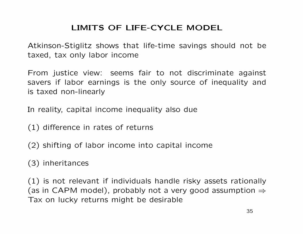
LIMITS OF LIFE-CYCLE MODEL

Atkinson-Stiglitz shows that life-time savings should not betaxed, tax only labor income

From justice view: seems fair to not discriminate againstsavers if labor earnings is the only source of inequality andis taxed non-linearly

In reality, capital income inequality also due

(1) difference in rates of returns

(2) shifting of labor income into capital income

(3) inheritances

(1) is not relevant if individuals handle risky assets rationally(as in CAPM model), probably not a very good assumption ⇒Tax on lucky returns might be desirable

35

SHIFTING OF LABOR / CAPITAL INCOME

In practice, difficult to distinguish between capital and laborincome [e.g., small business profits, professional traders]

Differential tax treatment can induce shifting:

(1) US C-corporations vs S-corporations: shift from corporateincome (and subsequent realized capital gains) toward individ-ual business income [Gordon and Slemrod ’00]

(2) Carried interest in the US: hedge fund and private equityfund managers receive fraction of profits of assets they managefor clients. Those profits are really labor income but are taxedas realized capital gains

(3) Finnish Dual income tax system: taxes separately capitalincome at preferred rates since 1993: Pirttila and Selin SJE’11show that it induced shifting from labor to capital incomeespecially among self-employed

36

Theory: Shifting of Labor / Capital Income

Extreme case where government cannot distinguish at all be-

tween labor and capital income ⇒ Govt observes only wl+ rK

⇒ Only option is to have identical MTRs at individual level ⇒General income tax Tax = T (wl + rK)

With a finite shifting elasticity, differential MTRs for labor and

capital income taxation induce an additional shifting distortion

The higher the shifting elasticity, the closer the tax rates on

labor and capital income should be [Christiansen and Tuomala

ITAX’08, see also Piketty-Saez Handbook chapter ’13]

In practice, this seems to be a very important consideration

when designing income tax systems [especially for top incomes]

⇒ Strong reason for having τL = τK at the top

37

Taxation of Inheritances: Welfare Effects

Definitions: donor is the person giving, donee is the person

receiving

Inheritances and inter-vivos transfers raise difficult issues:

(1) Inequality in inheritances contributes to economic inequal-

ity: seems fair to redistribute from those who received inheri-

tances to those who did not

(2) However, it seems unfair to double tax the donors who

worked hard to pass on wealth to children

⇒ Double welfare effect: inheritance tax hurts donor (if donor

altruistic to donee) and donee (which receives less) [Kaplow,

’01]

38

Estate Taxation in the United States

Estate federal tax imposes a tax on estates above $5.5M ex-emption (only about .1% of deceased liable), tax rate is 40%above exemption (2013+)

Charitable and spousal giving are fully exempt from the tax

E.g.: if Bill Gates / Warren Buffet give all their wealth tocharity, they won’t pay estate tax

Support for estate tax is pretty weak (“death tax”) but publicdoes not know that estate tax affects only richest

Support for estate tax increase shots up from 17% to 53%when survey respondents are informed that only richest payit (Kuziemko-Norton-Saez-Stantcheva ’13 do an online Mturksurvey experiment)

39

Treatment example: Information about the Estate Tax

14

Taxation of Inheritances: Behavioral Responses

Potential behavioral response effects of inheritance tax:

(1) reduces wealth accumulation of altruistic donors (and hencetax base) [no very good empirical evidence, Slemrod-Kopczuk01]

(2) reduces labor supply of altruistic donors (less motivatedto work if cannot pass wealth to kids) [no good evidence]

(3) induces donees to work more through income effects (Carnegieeffect, decent evidence from Holtz-Eakin,Joulfaian,Rosen QJE’93)

Critical to understand why there are inheritances to decide onoptimal inheritance tax policy. 4 main models of bequests:(a) accidental, (b) bequests in the utility, (c) manipulativebequest motive, (d) dynastic

41

ACCIDENTAL BEQUESTS

People die with a stock of wealth they intended to spend onthemselves: Such bequests arise because of imperfect annuitymarkets

Annuity is an insurance contract converting lumpsum amountinto a stream of payments till end of life [insurance againstrisk of living too long]

Annuity markets are imperfect because of adverse selection[Finkelstein-Poterba EJ’02, JPE’04] or behavioral reasons [in-ertia, lack of planning]

Public retirement programs [and defined benefit private pen-sions] are in general mandatory annuities

Newer defined contribution private pensions [401(k)s in theUS] are in general not annuitized

42

ACCIDENTAL BEQUESTS

Bequest taxation has no distortionary effect on behavior ofdonor and can only increase labor supply of donees (throughincome effects) ⇒ strong case for taxing bequests heavily

Kopczuk JPE ’03 makes the point that estate tax plays therole of a “second-best” annuity:

Estate tax paid by those who die early, and not by those whodie late ⇒ Implicit insurance against risk of living too long

Wealth loving: Same tax policy conclusion arises if donorshave wealth in their utility function [social status or power,Carroll ’98]

Kopczuk-Lupton REStud’07 shows that only 1/2 of peopleaccumulate wealth for bequest motives

43

Bequests in the Utility: Warm Glow Or Altruistic

u(c)−h(l)+δv(b) where c is own consumption, l is labor supply,

and b is net-of-tax bequests left to next generation and v(b)

is warm glow utility of bequests

Budget with no estate tax: c+ b/(1 + r) = wl− TL(wl)

Budget with bequest tax at rate τB: c+ b/[(1 + r)(1− τB)] =

wl− TL(wl)

Suppose first that b is not bequeathed but used for “after-

life” consumption [e.g., funerary monument of no value to

next generation]

⇒ Atkinson-Stiglitz implies that b should not be taxed [τB = 0]

and that nonlinear tax on wl is enough for redistribution

44

Bequests in the Utility: Warm Glow Or Altruistic

Suppose now that b is given to a heir who derives utility vheir(b)⇒ b creates a positive externality (to donee) and hence shouldbe subsidized ⇒ τB < 0 is optimal

Kaplow ’01 makes this point informally

Farhi-Werning QJE’10 develop formal model of non-linear Pigou-vian subsidization of bequests with 2 generations and socialWelfare:

SWF =∫

[u(c)− h(l) + δv(b) + vheir(b)]f(w)dw

The marginal external effect of bequests is dvheir/db and henceshould be smaller for large b

⇒ Optimal subsidy rate is smaller for large estates ⇒ progres-sive estate subsidy

45

A-S Fails with Inheritances In General Equilibrium(Piketty-Saez ECMA’13)

Atkinson-Stiglitz applies when sole source of lifetime incomeis labor:

c+b(left)/(1+r) = wl−T (wl) (w = productivity, l = labor supply)

In GE, bequests provide an additional source of life-income:

c+ b(left)/(1 + r) = wl− T (wl) + b(received)

⇒ conditional on wl, high b(left) is a signal of high b(received)⇒ b(left) should be taxed even with optimal T (wl)

⇒ Two-dim. inequality requires two-dim. tax policy tool

Extreme example: no heterogeneity in productivity w butpure heterogeneity in bequests motives ⇒ bequest taxation isdesirable for redistribution

46

Piketty-Saez Simplified Optimal Inheritance Tax Model

Measure one of individuals, who are both bequests receivers

and bequest leavers (in ergodic general equilibrium)

Linear tax τB on bequests funds lumsump grant E

Life-time budget constraint: ci + bi = R(1− τB)bri + yLi + E

with ci consumption, bi bequests left, yLi inelastic labor in-

come, bri pre-tax bequests received, R = 1 + r generational

rate of return on bequests

Individual i has utility V i(c, b) with b = R(1 − τB)b net-of-tax

bequests left and solves

maxbi

V i(yLi+E+R(1−τB)bri−bi, Rbi(1−τB))⇒ V ic = R(1−τB)V ib

47

Piketty-Saez ECMA’13 Optimal Inheritance Tax

Government budget constraint is E = τBb with b aggregate(=average) bequests. Govt solves:

maxτB

∫iωiV

i(yLi + τBb+R(1− τB)bri − bi, Rbi(1− τB))

with ωi ≥ 0 Pareto weights

Meritocratic Rawlsian criterion: maximize welfare of those re-ceiving no inheritances with uniform social marginal welfareweight ωiV

ic among zero-receivers

(e.g., people not responsible for bri but responsible for yLi) ⇒

Optimal inheritance tax rate: τB =1− b

1 + eB

with eB = 1−τBb

dbd(1−τB) elasticity of aggregate bequests and

b =E[bi|bri=0]

b relative bequest left by zero-receivers

48

Piketty-Saez ECMA’13 Optimal Inheritance Tax: Proof

SWF =∫iωiV

i(yLi + τBb− bi, Rbi(1− τB))

[NB: removed term R(1− τB)bri because ωi = 0 when bri = 0]

0 =dSWF

dτB=∫iωi ·

(V ic

[b− τB

db

d(1− τB)

]−RbiV ib

)⇒

0 =∫iωi ·

(V ic · b

[1−

τB1− τB

eB

]−

bi1− τB

V ic

)⇒

0 = b

[1−

τB1− τB

eB

]−

1

1− τB·∫i ωiV

ic · bi∫

i ωiVic⇒

as ωiVic ≡ 0 for bri > 0 and ωiV

ic ≡ 1 for bri = 0 ⇒

0 = 1− τB − τB · eB −E[bi|bri = 0]

b⇒ τB =

1− b1 + eB

49

Piketty-Saez ECMA’13 Optimal Inheritance Tax

Optimal inheritance tax rate: τB =1− b

1 + eB

1) Optimal τB < 1/(1 + eB) revenue maximizing rate becausezero-receivers care about bequests they leave

2) τB = 0 if b = 1 (i.e, zero-receivers leave as much bequestas average)

3) If bequests are quantitatively important, highly concen-trated, and low wealth mobility then b << 1

4) Empirically eB small (Kopcuzk-Slemrod ’01) but poorlyknown, b = 2/3 in US (SCF data) but poorly measured

5) Formula can be extended to other social criteria, elasticlabor supply, wealth loving preferences, altruistic preferences[see Piketty-Saez ECMA’13]

50

Optimal Capital Stock and Modified Golden Rule

Modified Golden Rule: r = δ + γ · gwith r = FK(K,L) = f ′(k) rate of return, δ discount rate, γ

curvature of u′(c) = c−γ, g growth rate (per capita).

Proof: $1 extra in period t gives social welfare u′(ct)

$1 + r extra in period t+ 1 gives social welfare(1+r)u′(ct+1)

1+δ =

(1+r)u′(ct)1+δ

u′(ct+1)u′(ct)

= 1+r(1+δ)(1+g)γu

′(ct) ⇒ 1 + r = (1 + δ)(1 + g)γ

This is equivalent to r = δ + γ · g when the period is small.

QED.

Normatively δ = 0 seems justified. Small capital stock and

r > g desirable if γ is high [controversy Stern vs. Nordhaus]

51

Optimal Capital Stock and Modified Golden Rule

Modified Golden Rule: r = δ + γ · g

Bequest and capital taxes affect capital stock

However, if govt can use debt, it can control capital stock

If debt used to set optimal capital stock at the Modified GoldenRule) then effects of taxes on K stock can be ignored ⇒Optimal K stock and optimal redistribution are orthogonal

If K stock is not at Modified Golden Rule, then optimal K taxformulas include a corrective term

[see King 1980 and Atkinson-Sandmo 1980 in OLG life-cyclemodel, Piketty-Saez ECMA’13 for models with bequests]

In practice: no reason for MGR to hold, govts do not activelytarget K stock

52

MANIPULATIVE BEQUESTS

Parents use potential bequest to extract favors from children

Empirical Evidence: Bernheim-Shleifer-Summers JPE ’85 show

that number of visits of children to parents is correlated with

bequeathable wealth but not annuitized wealth of parents

⇒ Bequest becomes one additional form of labor income for

donee and one consumption good for donor

⇒ Inheritances should be counted and taxed as labor income

for donees

53

SOCIAL-FAMILY PRESSURE BEQUESTS

Parents may not want to leave bequests but feel compelledto by pressure of heirs or society: bargaining between parentsand children

With estate tax, parents do not feel like they need to give asmuch ⇒ parents are made better-off by the estate tax ⇒ Casefor estate taxation stronger [Atkinson-Stiglitz does not applyand no double counting of bequests]

Empirical evidence:

Aura JpubE’05: reform of private pension annuities in the USin 1984 requiring both spouses signatures when retiring workerdecides to get a single annuity or couple annuity: reform ↑sharply couple annuities choice

Equal division of estates [Wilhelm AER’96, Light-McGarry’04]: estates are very often divided equally but gifts are not

54

DYNASTIC MODEL OR INFINITE HORIZON

Special case of warm glow: Vt = u(ct, lt)+Vt+1/(1+δ) implies

V0 =∑t≥0

u(ct, lt)/(1 + δ)t

subject to∑t≥0

ct/(1 + r)t ≤∑t≥0

wtlt/(1 + r)t

Dynasty with Ricardian equivalence: consumption dependsonly on PDV of earnings of dynasty

Poor empirical fit:

1) Altonji-Hayashi-Kotlikoff AER’92, JPE’97 show that in-come shocks to parents have bigger effect on parents con-sumption than on kids consumption (and conversely)

2) Temporary tax cut debt financed [fiscal stimulus] shouldhave no impact on consumption but actually do

55

INFINITE HORIZON MODEL: CHAMLEY-JUDD

Govt can collect taxes using linear labor income tax or capital

income taxes that vary period by period τ tL, τ tK

Goal of the government is to maximize utility of the dynasty

V0 =∑t

u(ct, lt)/(1+δ)t st∑t

qtct ≤∑t

qtwt(1−τ tL)lt+A0 (λ)

q0 = 1, ..., qt = 1/∏ts=1(1 + rs(1− τsK)), ...

With constant tax rate τK and constant r: Before tax price:

pt = 1/(1 + r)t and after-tax price qt = 1/(1 + r(1− τK))t ⇒

Price distortion qt/pt grows exponentially with time

56

CHAMLEY-JUDD: RESULTS

Chamley-Judd show that the capital income tax rate alwaystends to zero asymptotically: no capital tax in the long-run:

Two equivalent ways to understand this result:

(1) A constant tax on capital income creates an exponentiallygrowing distortion which is inefficient

(2) The PDV of the capital income tax base is infinitely elasticwith respect to ant increase in τK in the distant future [Piketty-Saez ’13]

Intuition: uc(ct+1)/uc(ct) = (1 + δ)/(1 + r(1− τK))⇒ savingsdecisions infinitely elastic to r(1− τK)− δ

If r(1 − τK) > δ, accumulate forever. If r(1 − τK) < δ, get indebt as much as possible.

57

ISSUES IN INFINITE HORIZON MODEL

1) Taxing initial wealth is most efficient [as this is lumpsumtaxation] ⇒ solutions typically bang-bang: tax capital as muchas possible early, then zero

2) Chamley-Judd tax is not time consistent: the governmentwould like to renege and start taxing capital again

3) Zero-long run tax result is not robust to using progressiveincome taxation [Piketty, ’01, Saez JpubE’13]

4) Dynastic model requires strong homogeneity assumptions(in discount rates) to generate reasonable steady states [un-likely to hold in practice]

5) Introducing stochastic shocks in labor/preferences in dy-nastic model leads to finite elasticities (and reasonable optimaltax rates) [Piketty-Saez ECMA’13]

58

NEW DYNAMIC PUBLIC FINANCE: REFERENCES

Dynamic taxation in the presence of future earnings uncer-

tainty

Recent series of papers following upon on Golosov, Kocher-

lakota, Tsyvinski REStud ’03 (GKT)

Principle can be understood in 2 period model: Diamond-

Mirrlees JpubE ’78 and Cremer-Gahvari EJ ’95

Generalized to many periods by GKT and subsequent papers

Simple exposition is Kocherlakota AER-PP ’04

Two comprehensive surveys: Golosov-Tsyvinski-Werning ’06

and Kocherlakota ’10 book59

NEW DYNAMIC PUBLIC FINANCE (NDPF)

Key ingredient is uncertainty in future ability w

2 period simple model:

(0) Everybody is identical in period 0: no work and consume

c0, period 0 utility is u(c0)

(1) Ability w revealed in period 1, work l and earn z = wl,

consume c1, period 1 utility u(c1)− h(l)

Total utility u(c0) + β[u(c1)− h(l)]

Rate of return r, gross return R = 1 + r

Discount rate β < 1

60

STANDARD EULER EQUATION

No govt intervention: c0 + c1/R = wl/R

Solve model backward (assume c0 given):

Period 1: c1 = wl−Rc0, choose l to maximize u(wl−Rc0)−h(l)

⇒ FOC wu′(wl−Rc0) = h′(l) ⇒ l∗ = l(w, c0)

Period 0: Choose c0 to maximize:

u(c0) + β∫

[u(wl∗ −Rc0)− h(l∗)]f(w)dw

FOC for c0 (using envelope condition for l∗)

u′(c0) = βR∫u′(c1)f(w)dw

This is called the Euler equation

61

MECHANISM DESIGN

Government would like to redistribute from high w to low w.

Government does not observe w but can observe c0, c1, z = wl

and can set taxes as a function of c0, c1, z

Equivalently (using revelation principle), govt can offer menu

(c0, c1(w), z(w))w and let individuals truthfully reveal their w

Govt program: choose menu (c0, c1(w), z(w))w to maximize:

SW = u(c0) + β∫

[u(c1(w))− h(z(w)/w)]f(w)dw st

1) Budget: c0 +∫c1(w)f(w)dw/R ≤

∫z(w)f(w)dw/R

2) Incentive Compatibility (IC): individual w prefers c0, c1(w), z(w)

to any other c0, c1(w′), z(w′)

62

INVERSE EULER EQUATION

Inverse Euler equation holds at the govt optimum:

1

u′(c0)=

1

βR·∫ 1

u′(c1(w))f(w)dw

Proof: small deviation in menus offered: ∆c0 = −ε/u′(c0)and ∆c1(w) = ε/[βu′(c1(w))] with small ε > 0

Does not affect individual utilities in any state:

u(c0 + ∆c0) + βu(c1(w) + ∆c1(w)) = u(c0) + βu(c1(w))

+∆c0u′(c0) + ∆c1(w)βu′(c1(w)) = u(c0) + βu(c1(w))

⇒ (IC) continues to hold and SW unchanged

Deviation must be budget neutral at optimum

⇒ −ε

u′(c0)+

1

R

∫εf(w)dw

βu′(c1(w))= 0

63

INTERTEMPORAL WEDGE

Jensen Inequality: for K(.) convex

⇒ K

(∫x(w)dF (w)

)<∫K(x(w))dF (w)

Apply this to K(x) = 1/x and x(w) = u′(c1(w)) ⇒

1∫u′(c1(w))f(w)dw

<∫

f(w)dw

u′(c1(w))=

βR

u′(c0)

⇒ u′(c0) < βR∫u′(c1(w))f(w)dw

⇒ Optimal govt redistribution imposes a positive tax wedge

on intertemporal choice

64

NDPF DECENTRALIZATION AND INTUITION

Decentralization: Optimum can be decentralized with a taxon capital income [which depends on current labor income]along with a nonlinear tax on wage income [KocherlakotaEMA’06]

Economic intuition: If high skill person works less (to imitatelower skill person), person would also like to reduce c0 andhence save more, so tax on savings is a good way to discourageimitation

Result depends crucially on rationality in inter-temporal choices+ income effects on labor: not clear yet how applicable thisis in practice

Would be valuable to explore empirically for example whetherDI (disability insurance) cheaters were saving more than noncheaters [would require merging SSA data and tax/wealthdata, hard to do]

65

NDPF NUMERICAL SIMULATIONS

Farhi-Werning ’11 propose numerical calibration and show that,for realistic parameters, the welfare gain of using full nonlinearoptimal capital/labor taxation is very small (0.1% in aggregatewelfare) relative to using only optimal labor taxation

Golosov-Troshkin-Tsyvinski ’11 also find on average small wel-fare gains and small optimal capital tax rates

⇒ Suggests that the mechanism is not quantitatively impor-tant even assuming the theory is right

⇒ Policy relevance of the NDPF for capital taxation likely tobe limited

DI/retirement application of NDPF might be quantitativelymore important

66

REFERENCES

Altonji, J., F. Hayashi, and L. Kotlikoff “Is the Extended Family Altru-istically Linked? Direct Tests Using Micro Data”, American EconomicReview, Vol. 82, 1992, 1177-98. (web)

Altonji, J., F. Hayashi and L. Kotlikoff “Parental Altruism and Inter VivosTransfers: Theory and Evidence”, Journal of Political Economy, Vol. 105,1997, 1121-66. (web)

Atkinson, A.B. and A. Sandmo “Welfare Implications of the Taxation ofSavings”, Economic Journal, Vol. 90, 1980, 529-49. (web)

Atkinson, A.B. and J. Stiglitz “The design of tax structure: Direct versusindirect taxation”, Journal of Public Economics, Vol. 6, 1976, 55-75.(web)

Atkinson, A.B. and J. Stiglitz Lectures on Public Economics, Chap 14-4New York: McGraw Hill, 1980. (web)

Auerbach, A. and L. Kotlikoff “Evaluating Fiscal Policy with a DynamicSimulation Model”, American Economic Review, May 1987, 4955. (web)

Aura, S. “Does the Balance of Power Within a Family Matter? The Caseof the Retirement Equity Act”, Journal of Public Economics, Vol. 89,2005, 1699-1717. (web)

67

Banks J. and P. Diamond “The Base for Direct Taxation”, IFS WorkingPaper, The Mirrlees Review: Reforming the Tax System for the 21stCentury, Oxford University Press, 2009. (web)

Bernheim, B. D., A. Shleifer, and L. Summers “The Strategic BequestMotive”, Journal of Political Economy, Vol. 93, 1985, 1045-76. (web)

Carroll, C. “Why Do the Rich Save So Much?”, NBER Working Paper No.6549, 1998. (web)

Chamley, C. “Optimal Taxation of Capital Income in General Equilibriumwith Infinite Lives”, Econometrica, Vol. 54, 1986, 607-622. (web)

Christiansen, Vidar and Matti Tuomala “On taxing capital income withincome shifting”, International Tax and Public Finance, Vol. 15, 2008,527-545. (web)

Cremer, H. and F. Gahvari “Uncertainty and Optimal Taxation: In defenseof Commodity Taxes”, Journal of Public Economics, Vol. 56, 1995, 291-310. (web)

Davies, J. and A. Shorrocks, Chapter 11 The distribution of wealth, In:Anthony B. Atkinson and Francois Bourguignon, Editor(s), Handbook ofIncome Distribution, Elsevier, 2000, Vol. 1, 605-675. (web)

DeLong, J.B. “Bequests: An Historical Perspective,” in A. Munnell, ed.,The Role and Impact of Gifts and Estates, Brookings Institution, 2003(web)

Diamond, P. and J. Mirrlees “A Model of Social Insurance with VariableRetirement”, Journal of Public Economics, Vol. 10, 1978, 295-336. (web)

Diamond, Peter and Emmanuel Saez “The Case for a ProgressiveTax: From Basic Research to Policy Recommendations”, Journalof Economic Perspectives, 25(4), Fall 2011, 165-190. (web)

Diamond, P. and J. Spinnewijn “Capital Income Taxes with HeterogeneousDiscount Rates”, NBER Working Paper, No. 15115, 2009. (web)

Farhi E. and I. Werning “Progressive Estate Taxation”, Quarterly Journalof Economics, Vol. 125, 2010, 635-673. (web)

Farhi E. and I. Werning “Capital Taxation: Quantitative Explorations ofthe Inverse Euler Equation,” forthcoming Journal of Political Economy2011. (web)

Feldstein, M. “The Welfare Cost of Capital Income Taxation”, Journal ofPolitical Economy, Vol. 86, 1978, 29-52. (web)

Finkelstein A. and J. Poterba, “Adverse Selection in Insurance Markets:Policyholder Evidence from the U.K. Annuity Market”, Journal of PoliticalEconomy, Vol. 112, 2004, 183-208. (web)

Finkelstein A. and J. Poterba, “Selection Effects in the United KingdomIndividual Annuities Market”, The Economic Journal, Vol. 112, 2002,28-50. (web)

Gale, William G. and John Karl Scholz, “Intergenerational Transfers andthe Accumulation of Wealth”, Journal of Economic Perspectives, Vol.8(4), 1994 145-160. (web)

Golosov, M., N. Kocherlakota and A. Tsyvinski “Optimal Indirect andCapital Taxation”, Review of Economic Studies, Vol. 70, 2003, 569-587.(web)

Golosov, M. and A. Tsyvinski “Designing Optimal Disability Insurance: ACase for Asset Testing”, Journal of Political Economy, Vol. 114, 2006,257-279. (web)

Golosov, Mikhail, Maxim Troshkin, and Aleh Tsyvinski 2011. “OptimalDynamic Taxes.” Princeton Working Paper (web)

Golosov, M., M. Troshkin, A. Tsyvinski and M. Weinzierl “Preference Het-erogeneity and Optimal Commodity Taxation”, MIMEO Yale, July 2011.(web)

Golosov, M., A. Tsyvinski and I. Werning “New Dynamic Public Finance:a User’s Guide” NBER Macro Annual 2006. (web)

Gordon, R.H. and J. Slemrod “Are “Real” Responses to Taxes SimplyIncome Shifting Between Corporate and Personal Tax Bases?,” NBERWorking Paper, No. 6576, 1998. (web)

Holtz-Eakin, D., D. Joulfaian and H.S. Rosen “The Carnegie Conjecture:Some Empirical Evidence”, Quarterly Journal of Economics Vol. 108, May1993, pp.288-307. (web)

Judd, K. “Redistributive Taxation in a Simple Perfect Foresight Model”,Journal of Public Economics, Vol. 28, 1985, 59-83. (web)

Kaplow, L. “A Framework for Assessing Estate and Gift Taxation”, inGale, William G., James R. Hines Jr., and Joel Slemrod (eds.) Rethinkingestate and gift taxation Washington, D.C.: Brookings Institution Press,2001. (web)

Kaplow, L. “On the undesirability of commodity taxation even when in-come taxation is not optimal”, Journal of Public Economics, Vol.90, 2006,1235-1260. (web)

Kennickell, A. “Ponds and streams: wealth and income in the U.S., 1989 to2007”, Board of Governors of the Federal Reserve System (U.S.), Financeand Economics Discussion Series: 2009-13, 2009. (web)

King, M. “Savings and Taxation”, in G. Hughes and G. Heal, eds., PublicPolicy and the Tax System (London: George Allen Unwin, 1980), 1-36.(web)

Kocherlakota, N. “Wedges and Taxes”, American Economic Re-view, Vol. 94, 2004, 109-113. (web)

Kocherlakota, N. “Zero Expected Wealth Taxes: A Mirrlees Approach toDynamic Optimal Taxation”, Econometrica, Vol.73, 2005. (web)

Kocherlakota, N. New Dynamic Public Finance, Princeton University Press:Princeton, 2010.

Kopczuk, W. “The Trick Is to Live: Is the Estate Tax Social Security forthe Rich?”, The Journal of Political Economy, Vol. 111, 2003, 1318-1341.(web)

Kopczuk, Wojciech “Taxation of Intergenerational Transfers and Wealth”,in A. Auerbach, R. Chetty, M. Feldstein, and E. Saez (eds.), Handbook ofPublic Economics, Vol. 5 (Amsterdam: North-Holland, 2013). (web)

Kopczuk, Wojciech and Joseph Lupton 2007. “To Leave or Not to Leave:The Distribution of Bequest Motives,” Review of Economic Studies, 74(1),207-235. (web)

Kopczuk, Wojciech and Emmanuel Saez “Top Wealth Shares in the UnitedStates, 1916-2000: Evidence from Estate Tax Returns”, National TaxJournal, 57(2), Part 2, June 2004, 445-487. (web)

Kopczuk, Wojciech and Joel Slemrod, “The Impact of the Estate Tax onthe Wealth Accumulation and Avoidance Behavior of Donors”, in William

G. Gale, James R. Hines Jr., and Joel B. Slemrod (eds.), Rethinking Estateand Gift Taxation, Washington, DC: Brookings Institution Press, 2001,299-343. (web)

Kotlikoff, L. “Intergenerational Transfers and Savings”, Journal of Eco-nomic Perspectives, Vol. 2, 1988, 41-58. (web)

Kotlikoff, L. and L. Summers “The Role of Intergenerational Transfers inAggregate Capital Accumulation”, Journal of Political Economy, Vol. 89,1981, 706-732. (web)

Kuziemko, Ilyana, Michael I. Norton, Emmanuel Saez, and Stefanie Stantcheva“How Elastic are Preferences for Redistribution? Evidence from Random-ized Survey Experiments,” NBER Working Paper No. 18865, 2013. (web)

Laroque, G. “Indirect Taxation is Superfluous under Separability and TasteHomogeneity: A Simple Proof”, Economic Letters, Vol. 87, 2005, 141-144. (web)

Light, Audrey and Kathleen McGarry. “Why Parents Play Favorites: Ex-planations For Unequal Bequests,” American Economic Review, 2004,v94(5,Dec), 1669-1681. (web)

Modigliani, F. “The Role of Intergenerational Transfers and Lifecyle Sav-ings in the Accumulation of Wealth”, Journal of Economic Perspectives,Vol. 2, 1988, 15-40. (web)

Norton, M. and D. Ariely “Building a Better America–One Wealth Quintileat a Time”, Perspectives on Psychological Science 2011 6(9). (web)

Park, N. “Steady-state solutions of optimal tax mixes in an overlapping-generations model”, Journal of Public Economics, Vol. 46, 1991, 227-246.(web)

Piketty, Thomas 2000. “Theories of Persistent Inequality and Intergener-ational Mobility”, In Atkinson A.B., Bourguignon F., eds. Handbook ofIncome Distribution, (North-Holland). (web)

Piketty, T. “Income Inequality in France, 1901-1998”, CEPR DiscussionPaper No. 2876, 2001 (appendix with optimal capital tax point). (web)

Piketty, T. “Income Inequality in France, 1901-1998”, Journal of PoliticalEconomy, Vol. 111, 2003, 1004-1042. (web)

Piketty, T. “On the Long-Run Evolution of Inheritance: France 1820-2050”, Quarterly Journal of Economics, 126(3), 2011, 1071-1131. (web)

Piketty, Thomas, Capital in the 21st Century, Cambridge: Harvard Uni-versity Press, 2014, (web)

Piketty, Thomas, Gilles Postel-Vinay and Jean-Laurent Rosenthal, “Inher-ited vs. Self-Made Wealth: Theory and Evidence from a Rentier Society(1872-1927),” Explorations in Economic History, 2014. (web)

Piketty, T. and E. Saez “Income Inequality in the United States, 1913-1998”, Quarterly Journal of Economics, Vol. 118, 2003, 1-39. (web)

Piketty, T. and E. Saez “A Theory of Optimal Capital Taxation”, NBERWorking Paper No. 17989, 2012. (web)

Piketty, T. and E. Saez “A Theory of Optimal Inheritance Taxa-tion”, Econometrica, 81(5), 2013, 1851-1886. (web)

Piketty, T. and G. Zucman “Capital is Back: Wealth-Income Ratios inRich Countries, 1700-2010”, Quarterly Journal of Economics, 2014 (web)

Piketty, T. and G. Zucman “Wealth and Inheritance in the Long-Run”,Handbook of Income Distribution, Volume 2, Elsevier-North Holland, 2014(web)

Pirttila, Jukka and Hakan Selin, “Income shifting within a dual income taxsystem: evidence from the Finnish tax reform,” Scandinavian Journal ofEconomics, 113(1), 120-144, 2011. (web)

Saez, E. “Optimal Capital Income Taxes in the Infinite Horizon Model”,Journal of Public Economics, 97(1), 2013, 61-74. (web)

Saez, E. “The Desirability of Commodity Taxation under Nonlinear IncomeTaxation and Heterogeneous Tastes”, Journal of Public Economics, Vol.83, 2002, 217-230. (web)

Saez, E. and G. Zucman “The Distribution of US Wealth, Capital Incomeand Returns since 1913”, Working Paper 2014 (in progress), preliminaryslides (web)

Sandmo, A. “The Effects of Taxation on Savings and Risk-Taking”, in A.Auerbach and M. Feldstein, Handbook of Public Economics vol. 1, chapter5, 1985, 265-311. (web)

Scholz, J. “Wealth Inequality and the Wealth of Cohorts”, University ofWisconsin, mimeo,2003. (web)

Slemrod, J. and J. Bakija, Taxing Ourselves: A Citizen’s Guide to theDebate over Taxes. The MIT Press, 2004.

Wilhelm, Mark O. “Bequest Behavior and the Effect of Heirs’ Earnings:Testing the Altruistic Model of Bequests,” American Economic Review,86(4), 1996, 874-892. (web)

Zucman, G. “The Missing Wealth of Nations: Are Europe and the USNet Debtors or Net Creditors”, Quarterly Journal of Economics, 2013,1321-1364. (web)

Zucman, G. La Richesse Cachee des Nations, Paris: Seuil, 2012 [trans-lation in english in 2015], summary in Journal of Economic Perspectives,2014 (web)

Zucman, Gabriel, “Taxing Offshore Wealth and Profits,” Journal of Eco-nomic Perspectives 28(3), 2014.