-L AGARD-CP-27S

U

Oh D I O Y H U -AE "P..*S A C i'C O M N

I t %7 4t1 FA C

JU01

D15Th! 3UYION STATEMENT AJJ 0~8

Ap:- -vnd for p'.)c vxlosc;

DISTRIBUTION AND AVAILABILITYON BACK COVER

I LLAGARD-CP-275

NORTH ATLANTIC TREATY ORGANIZATION

ADVISORY GROUP FOR AEROSPACE RESEARCH AND DEVELOPMENT

(ORGANISATION DU TRAITE DE L'ATLANTIQUE NORD)

AGARD)FC0_nference 4 roceedings, o.275

C COMBUSTOR MODELLING,,

JUL 10 1980.

~A

NTIS

Justi fiation_

By_

Dist '4butioI.L

Aw i)-qb iS odegikyail and/or

--'" St special

Papers presented at the Propulsion and Energetics Panel 54th (B) Specialists' Meeting,held at DFVLR, Cologne, Germany, on 3-5 October 1979.

Z/ ..

THE MISSION OF AGARD

The mission of AGARD is to bring together the leading personalities of the NATO nations in the fields of scienceand technology relating to aerospace for the foliowing purposes:

- Exchangirjg of scientific and technical information;

- Continuously stimulatingadvances in the aerospace sciences relevant to strengthening the common defenceposture;

- Improving the co-operation among member nations in aerospace research and development;

- Providing scientific and technical advice and assistance to the North Atlantic Military Committee in the fieldof aerospace research and development;

- Rendering scientific and technical assistance, as requested, to other NATO bodies and to member nations in

connection with research and development problems in the aerospace field;

- Providing assistance to member nations for the purpose of increasing their scientific and technical potential;

- Recommending effective ways for the member nations to use their research and development capabilities forthe common benefit of the NATO community.

The highest authority within AGARD is the National Delegates Board consisting of officially appointed seniorrepresentatives from each member nation. The mission of AGARD is carried out through the Panels which arecomposed of experts appointed by the National Delegates, the Consultant and Exchange Programme and the AerospaceApplications Studies Programme. The results of AGARD work are reported to the member nations and the NATOAuthorities through the AGARD series of publications of which this is one.

Participation in AGARD activities is by invitation only and is normally limited to citizens of the NATO nations.

The content of this publication has been reprcduceddirectly from material supplied by AGARD or the authors.

Published February 1980

Copyright © AGARD 1980All Rights Reserved

ISBN 92-835-02604

I1° } Printed by Technical Editing andReproduction LtdHarford House, 7-9 Charlotte St, London, WIJP.1HD

PROPULSION AND ENERGETICS PANEL

CHAIRMAN: Dr J.DunhamNational Gas Turbine EstablishmentPyestockFarnboroughHai-ts GU14 OLS, UK

DEPUTY CHAIRMAN: Professor E.E.CovertDepartment of Aeronautics and AstronauticsMassachusetts Institute of TechnologyCambridge, Mass 02139

PROGRAM COMMITTEE

M.l'Ing. en Chef M.Pianko (Chairman) M. le Professeur Ch.HirschCoordinateur des Recherches en Turbo- Vrije Universiteit Brussel

Machines - ONERA Dept. de M~canique des Fluides29 Avenue de la Division Leclerc Pleinlaan 292320 Chltillon sous Bagneux, France 1050 Bruxelles, Belgique

Professor F.J.Bayley Dr D.K.HenneckeDean of the School of Engineering Motoren und Turbinen Union GmbH

and Applied Sciences Abt. EWThe University of Sussex Dachauerstrasse 665Falmer, Brighton BNI 9QT, UK D-8000 MUnchen 50, Germany

Professor F.E.C.Culick Professor R.MontiProfessor of Engineering and Applied Istituto di Aerodinamica

Physics UniversitO degli StudiCalifornia Institute of Technology Piazzale Tecchio .0Pasadena, California 91125, US 80125 Napoli, Italy

HOST NATION COORDINATOR

Professor Dr Ing.G.WinterfeldDFVLRInstitut ftir Antriebstechn.ikPostfach 90 60 58

S[ : ID-5000 Kbln 90, German-y

PANEL EXECUTIW

Dr Ing.E.Riesterf-.

ACKNOWLEDGEMENT

The Propulsion and Energetics Panel wishes to express its thanks to theGerman National Delegates to AGARD for the invitation to hold its 54thMeeting in Cologne, and for the personnel and facilities made available for

' . this meeting.

V-<

yCONTENTS '

Page

PROPULSION AND ENERGETICS PANEL iii

Reference

SESSION I - SURVEY

MODELISATION DES FOYERS DE TURBOREACTEURS: POINT DE VUED'UN MOTORISTE

par Ph.Gastebois I

FUNDAMENTAL MODELLING OF MIXING, EVAPORATION AND KINETICS INGAS TURBINE COMBUSTORS

by J.Swithenbank, A.Turan, P.G.Felton and D.B.Spalding 2

Paper 3 not presented

SESSION II - BASIC PHENOMENA (PART I)

MATHEMATICAL MODELLING OF GAS-TURBINE COMBUSTION CHAMBERSby W.P.Jones and J.J.McGuirk 4

A PREDICTION MODEL FOR TURBULENT DIFFUSION FLAMES INCLUDINGNO-FORMATION

by J.Janicka and W.Kollmann 5

TURBULENT REACTION AND TRANSPORT PHENOMENA IN JET FLAMESby H.Eickhoff, K.Grethe and F.Thiele 6

ON THE PREDICTION OF TEMPERATURE PROFILES AT THE EXIT OF ANNULARCOMBUSTORS

by O.M.F.Elbahar and S.L.K.Wittig 7

Paper 8 not presented

SECOND-ORDER CLOSURE MODELING OF TURBULENT MIXING AND REACTINGFLOWS

by A.K.Varma, G.Sandri and C.duP.Donaldson 9

COMBUSTOR MODELLING FOR SCRAMJET ENGINESby J.P.Drummnond, R.C.Rogers and J.S.Evans 10

SESSION II - BASIC PHENOMENA (PART I1)

DEVELOPMENT AND VERIFICATION OF RADIATION MODELSby H.Bartelds 11

ASSESSMENT OF AN APPROACH TO THE CALCULATION OF THE FLOW PROPERTIESOF SPRAY-FLAMES

by Y.EI Banhawy and J.H.Whitelaw 12

FUNDAMENTAL CHARACTERIZATION OF ALTERNATIVE FUEL EFFECTS INCONTINUOUS COMBUSTION SYSTEMS

by R.B.Edelman, A.Turan, P.T.Harsha, E.Wong and W.S.Blazowski 13

CHEMICAL KINETIC MODELLING FOR COMBUSTION APPLICATIONby F.L.Dryer and C.K.Westbrook 14

COALESCENCE/DISPERSION MODELLING OF GAS TURBINE COMBUSTORSby D.T.Pratt 15i

CONTENTS I

Page

PROPULSION AND ENERGETICS PANEL ii

-/ Reference

SESSION I - SURVEY. __

MODELISATION DES FOYERS DE TURBOREACTEURS: POINT DE VUED'UN MOTORISTE

par Ph.Gastebois

FUNDAMENTAL MODELLING OF MIXING, EVAPORATION AND KINETICS INGAS TURBINE COMBUSTORS

by J.Swithenbank, A.Turan, P.G.Felton and D.B.Spading 2

Paper 3 not presented

SESSION 11 -7BASIC PHENOMENA (PART I)

MATHEMATICAL MODELLING OF GAS-TURBINE COMBUSTION CHAMBERSby W.P.Jones and J.J.McGuirk 4

A PREDICTION MODEL FOR TURBULENT DIFFUSION FLAMES INCLUDINGNO-FORMATION

by J.Janicka and W.Kollmann

TURBULENT REACTION AND TRANSPORT PHENOMENAIN JET FLAMESby H.Eickhoff, K.Grethe and F.Thiele 6

ON THE PREDICTION OF TEMPERATURE PROFILES'AT THE EXIT OF ANNULARCOMBUSTORS I

by O.M.F.Elbahar and S.L.K.Wittig

Paper 8 not presented /

SECOND-ORDER CLOSURE MODELING OF1TURBULENT MIXING AND REACTINGFLOWS

~/ by A.K.Varma, G.Sandri and C~duP.Donaldson 9

COMBUSTOR MODELLING FOR SCRAMJET ENGINESby J.P.Druminond, R.C.Rogers and;J.S.Evans 10

~~SES,'.)ION 11 - BASIC PHENOMENA (PART I1) .

DEVELOPMENT AND VERIFICATION OF RADIATION MODLS

by H.Bartelds

ASSESSMENT OF AN APPROACH TO THE CALCULATION OF THE FLOW PROPERTIESOF SPRAY-FLAMES

by Y.EI Banhawy and J.H.Whitelaw 12

FUNDAMENTAL CHARACTERIZATION OF ALTERNATIVE FUEL EFFECTS IN~CONTINUOUS COMBUSTION SYSTEMS

by R.B.Edelman, A.Turan, P.T.Harsha, E:Wong and W.S.Blazowski 13

CHEMICAL KINETIC MODELLING FOR COMBUSTION APPLICATIONby F.L.Dryer and C.K.Westbrook 14

COALESCENCE/DISPERSION MODELLING OF GAS TURBINE COMBUSTORSr by D.T.Pratt 15

Reference

S.- ..... SESSION III - TRANSIENT PHENOMENA AND INSTABILITIES .

MODELISATION DE ZONES DE COMBUSTION EN REGIME INSTATIONNAIREpar F.Hirsinger et H.Tichtinsky 16

ANALYSIS OF LOW-FREQUENCY DISTURBANCES IN AFTERBURNERSby F.E.Marble, M.V.Subbaiah and S.M.Candel 17

SESSION IV - FURNACES AND BOILERS .

SURVEY ON PREDICTION PROCEDURES FOR THE CALCULATION OF FURNACE IPERFORMANCE 'I

by J.B.Michel, S.Michelfelder and R.Payne 18

" NUMERICAL ANALYSIS AND EXPERIMENTAL DATA IN A CONTINUOUS FLOWCOMBUSTION CHAMBER: A COMPARISON

by F.Gamma, C.Casci, A.Coghe and UGhezzi 19

*MODELISATION DES FOURS ALIMENTES A L'AIR ENRICHI EN OXYGENEpar R.Guenot, A.Ivernel, F.C.Lockwood et A.P.Salooja 20

AN EFFECTIVE PROBABILISTIC SIMULATION OF THE TURBULENT FLOW ANDCOMBUSTION IN AXISYMMETRIC FURNACES.

by Th,T.A.Paauw, A.J.Stroo and C.W.J.Van'Koppen 21

MODELISATION MATHEMATIQUE"DU FONCTIONNEMENT DES CHAUDIERESDE CHAUFFAGE

par E.Perthuis 22

SESSION V - GAS TURBINE COMBUSTORS AND R/H SYSTEMS ..

A CHEMICAL REACTOR MODEL AND ITS APPLICATION TO A PRACTICAL COMBUSTORby W.Krockow, B.Simon and E.C.Parnell 23

SEMI-EMPIRICAL CORRELATIONS FOR GAS TURBINE EMISSIONS, IGNITION, ANDFLAME STABILIZATION

by A.M.Mellor 24

COMBUSTION MODELLING WITHIN GAS TURBINE ENGINES, SOME APPLICATIONS" ;'"AND LIMITATIONS

., ,by JOdgers 2SETUDE DE L'AERODYNAMIQUE D'UNE CHAMBRE DE COMBUSTION EN VUE D'UNE

, MODELISATION SEM!-EMPlRIQUEpar P.Hebrard et P.Magre 26

11

A_

MODELISATION DES FOYERS DE TURBOREACTEUPRS POINT DE VUE D'UN MOTORISTE

Ph. GASTEBOISChef du D6partemtent "COMBUSTION"

S.N.E.C.M.ACentre de Villaroche

j 77550 MOISSY CRAMAYEL - FRANCE

0 -RESUME

La mod~lisation des foyers de turbor6acteurs doit r~pondre A deux objectifs

-d'une part l'optimisation des foyers orient6e A l'heure actuello vers la r~duction des 6missions* polluantes ulais qui peut s'orienter vors l'optimisation des performances de stabilit6 ou de

N r6allurnage, et qui doit consid~rer los caract~ristiquos du syst~me dlinjection, de 1a zone rri-maire et de la dilution.

-d'autre part is pr~vision des performances des foyers; en projet qui doit permettre de pr~voirlot, caract6ristique3 des temp~ratures de sortie, des temp~raturos de paroi et des &,iissionspolluantes.

Pour r~pondre A ces deux objectifs, le motoriste souhaite deux types do mod6lisation, l'une simpiifi6epour estimer les performances, l'autre plus approfondie pour optimiser l'architecture des foyers.

Dans lea deux cas une meilloure connaissanco des ph~nom~nes physiques (rayonnement, transferts, cin6-tique chimique), grace A des mesures perfectionn~es est indispensable.

I -INTRODUCTION

La conception des foyers de turbor6acteurs est rest6e pendant de ncmbrouses ann~es un "art" pour loquoll'ing~nieur mettalt A profit l'exp6rience acquise et ln r6flexion fond~e sur des ideas simples pourapprocher les r~sultats recherch~a par 6tapes et modifications successives.

N~anmoins, it est apparu assez rapidement la nk~essit6 do pr6voir les performances des chambres decombustion en projet. Des 6tudes nombreuses ont Wt entreprises pour tenter par example de pr6voir leprofit radial des temp~ratures do sortie, le rendement do combustion ou les temp6ratures do paroi dufoyer en utilisant des mod~les a6rodynamiques et thermiques simples.

Cotte tendance s'ost accrue dautant plus quo le co~t des essais partiels s'est 61ev6 avec l~augrnenta-tion des niveaux do pression et do temptwature A Ventr6e des foyers.

La recherche du compromis n~cessaire pour tenir compto simultan~inent des contraintos do performancesclassi4ues at des contraintes do pollution a conduit on outre a recherchor A priori une optimisation dol'architecturo des foyers grace A unemodlisation do 1'ensemble du tube A flamme faisant intervenirdes mod~los plus perfectionn~s int~grant lea ph6nom~nes dle cin~tique chimique et do turbulence.

2 -OPTIMISATION DES FOYERS GRACE A LA MODELISATION

ae contr~intes do r~duction des 6missions d'esp~ces polluantes par lea chambres do combustion princi-plsdes turbor6acteurs ont conduit, soit A reconsid6rer llarchitecturo des foyers classiques on vue

d'optimisur la r~partition do l'air entre les diff6rentes zones du foyer et dfutiliser au mieux levolume dirponible, soit A concevoir de: foyers Ainjection 6tage o A g6omtrie variable pour lesquels

it mprtedeconatrela mole r partition do l'air et du carburant - Fig. 1.

La mod~lisation des foyers sls ~~~ tre 11ntuetidsesbeAuetolleopisaon

Les difficult~s rencontr~es pour mod~liser les foyers do turbor6actours proviennont do la n~cessit6 do* tenir compto sirnultankeent des ph~fiom~nes'do m~lango turbulent et des 6volutions chimiquos.

Do plus, it faut en outro pour slapprocher des foyers r~els d6crire la r~partition spatiale et l'6vapo-

rtiopn du combustbe. ogaisprrpota ep mqe ofyrpu

Uno piemi~re 6tape, simple at n~anmoin d~jA traps utile pour 1e motoristo, consiste A supposer quo les

A-- alors 6tre mod~lis6 par un assemblage do foyers homog~nes (Ref. 1, 2). On pourra concevoir par example

fz - d'une part une mod~lisation do la zone primairo permettant do connaltre 1'Avolution des indices dl~mis-sion a la sortie de la zone prinaire en fonctioni des param~tres a6rothermodynamiques et do la richossede fonctionnemeht et d'autre part unc mod~lisation do la zone do dilution qui jouo un role essential

dan: le proceasus de combustioin m~me dans les conditions du r~gime ralonti ou so forme la majeuro

priadu monoxydo do carborne et des hyqrocarbures iffbr~l~s.

La on pimir et bdli~epa u asebgedeoyars homognesonitdust ercrulin

Tutefois pour mieux appeocher les pef-formances du foyer, it est souhaitable d'Inclure tin 11r6acteur.dst'n" (R)porr elut'i n des gaz recirculants.

1-2

La zone de dilution est rcpyrisent6e par un r6acteur piston qui peut WtailIeurs 6galement 6tre SjMUl6par une suite de r~actours homog~nes de faibla volume unitairo - Fig. 2 et 3.

S'il est vrai que Il'awmlioration de la qttalit6 de la puly~risation par adoption dlinjecteurs a6rodyna-miques a pernis de se rapprocher senaibiement du cas o~i lea temps de m~lango et de vaporisation sontfaibles, les ph~nom~nos de m~lange ne peuvent 6tre compl~teniont n6§lig~s et nous pensons que la notionde foyers "bien m~lang~s" (W.S.R) dans lesquels le carburant et Ilair sont m~lang~s rapidement maispas instantan~ment constitue une 6tape susceptible dlapporter des ani~liorations notables (Ref. 3, 4, 5).

L'un des avantages de ces modles, hormis une certaine sieiplicit6 est que 1'ling6niour peut A partir deconsid~rations physiques simples, d'estimations ou de mosures du temps de s~jour dans lo foyer, d6ter-miner les volumes do chacun des foyers homog~nes entrant dana le mod~le ; il contr~le done relativementbien l'exactitude des hypoth~ses d'entr6e dans le mod~lo.

Danas le but d'optimiser l'architecturo des foyers, Ilintroduction des,.parametres relatifs A Ilinjectionet notammeht ceux relatifs a la r~partition du carburant Oans !a zone primaire Wes sans doute pasfonda 'montale dans une premiere 6tape. N6anmoins, si Ilon veut ppa- exemple slint6resser aux hydrocarbu-res imbrOl~s ou AL la formation des fum~es, il faudra, nous semble-t'il tenir compte effoctivemont deces param~tres et mod~liser alors do faqon d~taill6e les processus de m~lango, d'Avaporation du combus-tible ainsi quo lea premi~res 6tapes, de d~composition et de combustion du carburant.

La sch&,atisation par foyers homog~nes "parfaitement m~lang~s" ou mgme "bien m6lang6s" sera alorsinsuffisante et une mod~lisation tridimensionnelle plus compl~te sera alors n~cossaire. Le degr6 decomplexit6 auquol on est alors conduit rend ces m6thodes, At notre avis, d'un emploi syst~matiquedifficile dans 1'industrie.

* L'optimisation des foyers do rechauffe qui constitue 6gale~iont un objoctif essontial pour 1e motoristo* est accessible par une mod~lisation appropri~e d6 la zone de recirculation cr66e par l'accroche-flamme,

at de la propagation du front do flammo turbulent so d~veloppant en aval de l'accroche-flamme - VoirFig. 4.

Cotte mod~lisation doit permettre d'optimiser le nombre dlaccrocho-flammos afin dlobtenir le rendementdo rechauffe demand6 avec uno longueur de canal minimalo tout on satisfaisant aux crit~res de stabilit6at do Porte de charge.

LA encore, deux stados do complexit6 pouvent 6tro consid6r6sl d~n part un mod~le do combustion oi I'oni'ait Ilhypoth~so que Ilalr et le carburant sont pr6n'~lang6s on amont des accrocho-flammes, d'autro partun -od~le plus sophistiqu6 oil Ilon prond en compto cos pht~n':,nnes do m6lange et d'Avaporation du combos-tible.

tLos m~thodes do calculs compl~tos couplant les mod~les a6rodynamiques turbulents aux mod~les do i~iquo chiiniques aont sans douto los seulos dans ce c~s suscoptiblos do pormottre cotte optimisation.

3 -MODELISATION DES FOYERS EN PRO.IET

L'architecture 96n6rale du foyer 6tant d~finio, soit A partir do l'exp6rience ant~rieuro, soit A partirdo l'optlmisation par le calcul, il reste au motoriste A pr~ciser le dimensionnemont du foyer at Acalculer grace A dos 'nod~les appropri6s lea perfdrmancoa du foyer, tellos quo

- r~partition do Il'ar dana lea diff6rentos zones,

- pertes do charge,

- temp~ratures do paroi dana divers cas do fonctionnement,

- performances dp stabilit6,

- r~partition des temp6ratures do sortie,,

Porcaund e d ls fo e poluti s onrnt A doux probl~mos ;d'une pert il dolt choisir 10niveu d cooleit6 uqul i vaslarr~tor pour rendro compte avec un degr6 do confiance satisfaisantdesperormnce dofoyr ;dlatrapart, il doit dans tout modale rentrar un certain nombro do donn~es

initiales ou do coefficients ompiriques qu'il oat parfois difficile do connattro A priori.

ouexample, dens lo calcul do la r~partition des 06bits d'air dana 1e tube A !lamme, outre la g6om6-tri dotub aflammo et des orifices on pourra ou non tonir compte des profils do vitesse et do pros-

aiwzn A la sortie du diffuseur, on pourra calcuter ou non l'Acoulement autour de la tate do chambre pourintr~.dui--o l6a profits do prossion at de vitesse entre tube A flame et carters, etc. mais it faudradens toos lea cas-entrer los coefficients de d~bit des orifices et parfois los profils initiaux slils

Ce p1'ogrissae pourra Atre coupl4 avoc un mod~le de combustion plus ou momns simplifi6 afin do calculor lar~phrtition des d6bits d'air en combustion.

L'exp~rie%-ce acquise hous a montr6 quo des variations g~o'6triquos de d~tail pouvaient avoir des cons6-quences i'portantes Bur tn1ile ou tolle performance et coci nous incite A pensor quo, m~ne des mod~les-tris sophistiqu6s auront beaucoup do peine A pormettre des pr6visions quantitativos tr~s pr6cises.

Clest done, m~ame au-niveau du d~veloppement do f,-yer, principalement pour pr~voir Ileff'et d'une varia-tion do tel ou tel param~tre, le r~suttat de telle ou telle modification, ou recherchor quelte modifi-cation preta d'attaindre tel objectif, qo lo. constru-cteur utitisera la mod6lisation des toyers.

1-3

Citons par exemple l'importance relative des 6changes par rayonnement et convection dans 1'6quilibrothermique des parois dui foyer, la modification du profil radial d'un foyer par modification des per-(;ages do dilution etc.

Une m6thode s~duisante pdrmettanC d'aboutir au degr6 de cornplexit6 minimal, consiste ?i partir d'unemod~lisation tras sophistiqu6e, prenant en compte dans la mesuro eu possible, tous les ph6nom~nes a~ro-thormochimiques, puis i rechercher quelles simplifications peuvent 6tro r6alis6es sans remettre encause le r~sultat final.

Cette technique est employ6e dans la mod~lisation des ph~nom~nes de cin~tique chimique pour lesquolsiling6nieur peut reconnaitro sans difficult~s lea r6actions tras rapides des r6actions lentes et6tablir des mod~los "a 6quilibre partiel" ou "A.1,tat quasi stationnaire".

Son emjdoi sera certainejient utile dans lea mod~les a6rothermodynamiques tridimensionnels pour lesquelsles temps de calculs sent tr~s longs et peu compatibles avec une utilisation fr6quente comme peut enavoir besoin ic constnucteur.

La connaissance des valeurs initiales des variables dlentr6e dans los probl~mes de combustion turbu-lonte d'un m6lange air-carburant liqi'ide reste un des probl~mes importants ; en effet, plus la mod~li-sation des ph6nom~nes de m6lange turbulent est pouss6e plus 1'acc~s aux param~tres d'entr~e est (liffi-cile. Ceci est d'autant plus vrai que t'on sl6loigne des montages exp6rimentaux de recherche pourslint6resser aux foyers r~als des turbomachinem.

Un effort particulier doit donc C-tre port6 sur lea techniques do mesure, d'une part pour acqu6rirexp6rimcntalement 1cm donn~es de base n~cessaires au calcul maim aussi d'autro part pour n'introduiredans los mod~les quo des param~tres auxquels on sait avoir acc~s ou dent l'ordre do grandeur est suffi-sammont bien connu.

Le motoriste est 6videmment tr~s m~fiant devant des mod~les tr~s 61abor6s pour lesquols certaines"variables" sont choiaies en fonction do chaque cam d'application pour quo tc calcul recoupe l'exp6-rienco sans quo los lois ou los r~gles d~finissant ces variables soilent bien connues.

4-ETAr ACTUEL A LA SNECHA

4 Nous no d~crirons pas ici 10 centonu des mod~lisations utilis~es a la SNECMA mais tonterons plut~t dod6crire 1e processus do conception ot do misc au point dos foyers pour mettre en 6vidence les r6ussitemet les lacunes dos mod~les propos6s ainsi quo 1'6norme travail qui resto A faire.

Connaissant lea conditions do fonctionnoment ot los performances du foyer recherch6os, 1e motoristo va,A partir d'un certain nombre de crit~ires d6duits soit do l'exp6rience ant~rioure soit dos r6sultats des6tudos d'optimisation dent nous avons jparlo, so fixer une r6partition des d~bits d'air dans la zoneprimairo, la zone do dilution, les films do refroidissemont, lo syst~ime d~injectien ...

Un mod~ile do calcul a6rothermodynaniquo, avoc un schkma do combustion simplifi6 va permettre do calculor

los pergages du tube A fleame pour obtenir Jos caract6ristiquos recherch~es.

Un programme do calcul inverse, pormottant A partir de donn6es g6om6triquoa du tube A flamme de calculerla r6partition des d6bits dtair dans chacune des zones dui foyer ainsi quo ma porte do charge sort dobase aux modifications 6ventuelles sur celiti-ci.

Des mod~les do calcul de "performances" peuvont 8tro alors utilis6s. Ceux quo nouu pr6sentons sonx. soitop~rationnels, molt on cours do misc au point, soit objet do rechorches en vue do leur 6laboration.

Un mod~le do calcul des temp6r~tures de paroi des foyers rcfroidis pai- convection, film-cooling oumultiperforation permet do pr6voir los tomp6ratures do parei en foniction des diverses conditions dofonctionnemont et do s'asauror de la tonue thermique et dui la dur6e do vie du tube A flamme. Touterecherche aboutissant A une mejl~oure connaissance des caract~ristiques do rayennement des flamniesainsi quo la description des ph6nom~nes d'intoractinn couche-limite-jots tranavormaux permettra dtoperfectionner cc typo de mod6liaation.I Un modale do calcul do la r6partition des temp~ratures do sortie dui foyer est particuli~rement utile aumotoriste puisqu'il lui pormot d'adapter Ia r6partition des pergagem do dilution dui tube A flamac afind'obtenir le profil radial n6cossairo A la tenue thermique de la turbine. Los 6tudes portant sun 1e

m~lange des jets turbulents et aur los mathodes do calcul tridimensionnelles permettront d'affinor los

Enfin, essontielloment dans 1e domaine des motours civils, la pr6vision des niveaux do pollution pout

A une mod6lisation globalo tridimensionnelie. Dans ce domaine los rochorches fondamentalom concernaitla formation des polluants (CO, 11C, NOx, fum6es) moat indispensablem concurreanent. avec le d~volopp-mont des techniques do calcul, afin d'uno pert do mioux d6crire los 6tapes du combustion dui preduitcomplexe qu'est 1e k6ros~ne, d'autre part do mieux connattre les constantem do vitesse do r6action dams

une large 9amnse do temp6rature.

Nous pensons qu'une mod~lisation bas6e sur l'assomblage do foyers homog~nes (PSR) ou bien m~lar.96s (WSR),constitue une base do d6part int6ressante puisqulel'le permet dtenvisager des assemblages dent la comple-xit6 ira croissanto aui-fur-et-A-mesure quo -10 bosoin slen fera mentir et quo la connaissanco do l'a6ro-

j74 dynamique dui foyer et do !a r~partition dii carburmat dans 1e foyer slam6lioreront.

1-4

CONCLUSION

La mod6lisation des foyers est un outil tr~s utile au motoriste pour la mise au point des foyers,d'autant plus que le co~t des essais partiels staccrott avec l'Al6vation du taux de compression desmoteurs. L'int6rat port6 aux probl~mes de pollution a accru le besoin en mod~les-comportant aussibien une mod~lisation des ph~nom~nes a~rodynamiques et thermiques qu'une mod~lisation des 6volutionschimiques.

Le constructeur souhaite disioser de deux types de mod~les

-d'une part une mod~lisation globoale du foyer permettant d'optimiser les r6partitions d'air etde carburant entre les diff~rentes zones du foyer, pour utiliser le volume minimal tout enassurant un niveau de performances satisfaisant. Ces mod~les tout en restant assez simples pour6tre utilisables industriellement devront A l'avenir tenir compte de maniaro plus approfondiedes param~tres lis A l'injection.

-d'autre part des mod~les permnettant A partir de l'optimisation pr~c~donte de d~finir les donn~esg~om6triques du foyer et d'en estimor avec une bonne pr~cision los principales performancos.Dans ce but des mod~les Al1inentaires sp~cifiques et simplifi~s se r~v~lent tr~s utiles pour lemotoriste au cours du d~veloppemont du foyer.

Cependant dans los deux cam la pr~vision ou l'optimisation dos niveaux do pollution aminennt a onvisa-ger des mod~les dont le degr6 de sophistication ira croissant en maine temps quo la mod~lisationd6taill6e des processus a6rotho-mochimiques progressera.

En tous cas le motoriste insiste sur la n~cossit6 do connattre A priori ou par ilexp6rienco ant~rioure* tous los parana~tres d'entr6o figurant dans ces mod~hes. 11 nous paralt donc indispensable quo los

moyens de diagnostic et do inosures progressont en parall~ho avec los moyens do calcul.

* REFERENCES

1 - BORGHI R.Etude th6oriquo do l'optimisation do la combustion dans los foyers do turbomachinosActa Astronautica Vol 1 - 1974 - pp 667-685

2 - IIAKMOND D.C mnr ot MELLOR A.nAnalytical calculations for the performance and polluant emissions of gas turbino combustorsAIAA Paper 71-711

3 - OSGERDY I.TLiterature review of turbine combustor modeling and emissionsAIAA journal Vol 12 NO 6 Juin 1974k

4 - DEER J.M - LEE K.DThe effect of residence time distribution on the performance and efficiency of combhustor10th International Symposium on Combustion 1965 - PP 1187-1262

5 - SWITIIENBANK, J, POLL, I., VINCENT, l1.W. at WRIGHT, D.DCombustor Design Fundamentals -14th symposium (International) on Combustion 1972 -p 627

-..ZONE PRIMAIRE_ -ON.D

.AIR-.

,CARBURANLT E 0' NJECTIN.

- FOY ER A INJECTION -FOYER A INJECT IONETAGEE RADIALE-. ETAGEE AXIALE_

F~g.16]fig.1Cqfig. 2 ..SCHEMATISATION PAR FOYERS ELEMENTAIRES

.-SANS REC IRCULATION-..ASSEMBLAGE de FOYERS

MRFIEMENT .ASSEMBLAGE de FO(EMELANES EI'DE PARFAITEMENREACTEUR. PISTO N. MELANGES-.

(FPM+R P) ____

fig2A ~RBURANT J.B CAR BURANTEVENTUEL EVENTUEL

LR.M. FPM. RP Pm. ERM. -

FRBURANT. FJRBU'RANT.

-CARBURAN- .CABUNT

AVCAEIRURTON.

F.P.M F.PM. P P-P-~

REI CLZIONE ERCRUAIN

FaCEAIA ION -PR r____EEENAIE

AVEC RPROPCUGATION

-CARBURAABUANTURBULENT

IRR.1

I;;'-OERD RCAUF

I _

IF. P. RPM. p pP

RECI RCULATI ON

-SCHEIMAT ISAT ION -PAR FOYERS ELEMENTAIRE

AV-Q REIRCULATIQN-E- fig. 3*-

f ig.4T YOYER DE RECIHAUFFE..

4ZONE DE RECIRCULATION.

..CARBRANJ PGATIQN

[T MU LETE

1-7

DISCUSSION

C.Hirsch, Be(1) Quel est le contenu (degrd de complexitd, variables entrde-sortie, reprdsentation de la turbulence,... des

mod~les partiels utilisds (FPM- foyer parfaitement m~lang6; RP: rdacteur piston)?

(2) Sur quels crit~res sont basds le choix du nombre de mod~Ies partiels entrant dans la moddlisation d'un foyer?

Rdponse d'Auteur(1) En cc qui concerne les foyers liomog~nes (FPM) nous utilisons une cin6tique simplifi~e en ce qu'ellc comporte

une reaction global de decomposition du carburant, los donndes de cindtique chimique nous sont fournies pardes organismos de recherches, comme I'ONERA par exemple. En ce qui concorne les mod~les utilisds dans losr~acteurs pistons (RP) nous utilisons des constantes do cindtique diduites de nos essais partiels ou de la

(2) Le choix du nombro et de la nature des foyers 6l1nientaires rdsulte d'essais partiels dt~crivant les diffdrenteszones, les temps de sdjour et los volumes de chacune de ces zones; le debit d'air entrant dans chacun de cesfoyers rdsulte du calcul global de la r6partition des debits d'air et des dorndes prd6dentes.

M.Pianko, FrA tVon des preuves exptdrimentales, quo dans les foyers des turbo-rdactours, le temps physique et nettement infdrieurau temps chimique?

Rdponse d'AuteurNous avons compard les r6sultats expdrimentaux obtenus aver, un foyer reprdsentant une zone primaire soule et les

* rdsultats de calcul en assirnilant cette zone Ai un foyer liomog~ne. L'accord qualitatif entre ces rdsultats lorsquol'injcction ost du type adrodynamique est as(.,z bon pour justifier cette hypoth~se en premiere approximation.

M.Pianko, FrQuels sont, de faqon prdcise, los besoins d'amdlioration des t'clhniques et procdds de Inosure?

Rdponse, d'Auteur11 no suffit pas do vdrifier que ~es rdsultats de la modtdlisation sont en --.cord avec ceux obtenus Ai la sortie due foyer,ii nous parait indispensable de comparer les repartitions de vitosso, les intensitds do turbulence, los fluctuations dotempdrature et de concentrations obtenues par le calcul av'ec les valeurs mesurdos dans les foyers. C'ost dans ledomaine des mesures optiquos des vitesses, twnpdraturp et concentrations au scmn des foyers en combustion que doit,A notre avis, dtio portd l'effort.

N.Petezs, Geho crois A l'avenir des m~thodes traitant de l'interaction turbulp~nce-rdactions chimiques. Pour ]a turbulence ondispose des mod~les A deux dquations k - e ou du type lengueur de mdliange. Pour la cindtique chimique desreactions At tempdraturo d'activation dlevde on pout utiliser les m~triodes do d~veloppement asyinptotique qui ontdonnd do bons rdsultats pour la prediction do l'allumar. d'uno flamme do diffusion et la pr~diction dos oxydosd'azote. En g~ndral cos problmos no sont pas couples (6coulement turbulents non r~actifs ou flammos laminairos).Pouvoz-vous commeonter cos nouvelles mdthodes do calcul?

RWponse d'Auteur

~ I Nous sommos tr~s intdrossds par cos nouvollos m~thodes; mais comme vous le ditos olles no sont applicablos qu'A desj flamnmes simples alors quo nous traitons, dans nos foyers, d'dcouloments tridimensionnels avec injection do carburant

liquido.

Ii

2-I

FUNDAMENTAL MODELLING OF MIXING, EVAPORATION ANI XINETICF IN GAS TURBINE COMBUSTORS

J. Swithenbank A. Turan+ , P.G. Felton* and D.B. Spalding

* Department of Chemical Engineering and Fuel Technology, U: .rsity of Sheffield, Sheffield, S1 3JD.

+ Science Applications, Inc., Woodland Hills, California, 91364, U.S.A.

7- Department of Mechanical Engineering, Imperial Collage, Kensington, Londoa. S.W.7.

SUMMARv

The objective of this review is to highlight past achievements, current status and future prospectsof combustor modelling. The past achievements largely consists of detailed studies of idealized flameswhich have given an understanding of the relevant fundamental processes. However, gas turbine combustorcomputations must include the simultaneous interacting processes of three-dimensional t,.o-phase turbulentflow, evaporating droplets, mixing, radiation and chemical kinetics. At the present time numerical predic-tion algorithms are becoming available which can model all these processes to compute the hydrodynamic,thermodynamic and chemical quantities throughout a tnree-dimensional field. Complementary stirred reactornetwork algorithms permit the prediction of minor constituents (pollutants), again including such effectsas droplet evaporation and unmixedness. Expe:imental verification of these various predictions reveals re-markably good agreement b t=esn measured and predicted values of all parameters in spite of tl,a physicaland mathematical assumptions currently used. Future problems include: more accurate modelling of turbulence/kinetic interactions, numerical procedure optimization and detailed measurements of residence time distri-bution and two-phase parameters in real, hot combustors.

1. INTRODUCTION - PAST ACHIEVEYENTS

Presently the aviation industry produces a wide variety of engine designs,ranging from simple lift en-gines to sophisticated multispool by-pass engines. In so doing the combustion engineer has the importanttask of selecting the combustor design which yields maximum overall efficiency, while minimizing the emis-sion of pollutants.

Gas turbine combustors involve the simultaneous processes of three-dimensional turbulent flow, two-phase evaporating droplets, mixing, radiation and chemical kinetics. The complexity of these interactingprocesses is such that most current gas turbine combustor design methods depend largely on empirical corr-elations. However, current pressures to minimize pollutant formation, together with the foreseeable re-quirement to use more aromatic fuels, and even synthetic shale or coal derived fuels, suggest that theinitial stages of combustor design would be greatly facilitated by a comprehensive mathematical modelbased on fundamental principles.

Fortunately, the past achievements in combustion science, which large consist of detailed studies ofsimple laminar/turbulent, pre-mixed/diffusion, and single droplet flames, have given an understanding of

*the relevant fundamental processes. In modelling combustors, the problem is to write down a set of govern-ing differential equations, which correctly, or at least adequately, model interactions such as those be-tween turbulence and chemical kinetics, whose solution is within the capability of present computers.

It is beyond the scope of this paper to present all the models which have been developed, and theapproach used is to present some modelling procedures which are typical of the current 'state of the art'.A 'ey feature of this presentation is a critical comparison of the results of the prediction procedureswith experiment. Whilst this does not necessarily prove the validity of the mathematical models used, itdoes indicate the present capability, and future potential and promise of the techniques.

Previous studies of turbulent flow fields have predominantly considered two-dimensional isothermalflow. ;implifying assumptions which are made in the mathematical and physical stages of modelling willcertainly introduca errors and it has been demonstrated that the inherent constants used in the equationscannot ciaim true universalism. Nevertheless, although there are uncertainties associated with their use,many studies have shown that isothermal flow fields can be predicted with sufficient accuracy to be ofpractical value.

Models of turbulence employed in combustion situations have, on the other hand, frequently assumedextended forms of the isothermal cases, the flame/turbulence interaction being represented by simple ex-pressions lacking rigorous iormulation. Turbulence models are required because it is not possible to solvethe unsteady versions of the transport equations analytically, and their numerical evaluation is well be-yond th. capabilities of present computers. Since we notmally only require the time averaged flow for en-gineering purposes, the problem reduces to the representation of the statistical correlation terms, whichappear in the time averaged versions of the transport equations, in terms of known quantities. In the first

, part of this paper, the two equation (k,t) anodel of turbulence has been used although its validity in hotreacting flows has not yet been firmly established. ilst higher order models would probably be requiredfor strong flows for examhpye, in the present case the two equation model was considered to bethe lowest level of closure which would give.adequate accuracy.

In the second part of the paper, contrary to the rigorous description employed in the finite differencemodelling by partial differential equations of heat, mass and momentum transfer, the, "Chemical ReactorModelling" approach concentrates on the representation of the combustor flow field in terms of interconnected'-I partially stirred and plug flow reactors. This approach has the advantage that the complex, time-consumingsolution of the equationa is replaced by simple flow models and the computational requirements are generallyminimum. These features enable the attractiveness of chemical reactor modelling to be exploited during thedevelopment phase of combustor design.

2. FINITE DIFFERENCE PROCEDURE FOR AERODYNAMIC AND TIERMAL PREDICTIONS

The finite difference procedure employed in this work is derived from the pioneering work at ImperialCollege, (1,2,3,4,5) It uses the cylindrical polar system of coDrdinates to predict the complex three-

dimefsional swirling and reacting flow inside a co bustor.

2-2

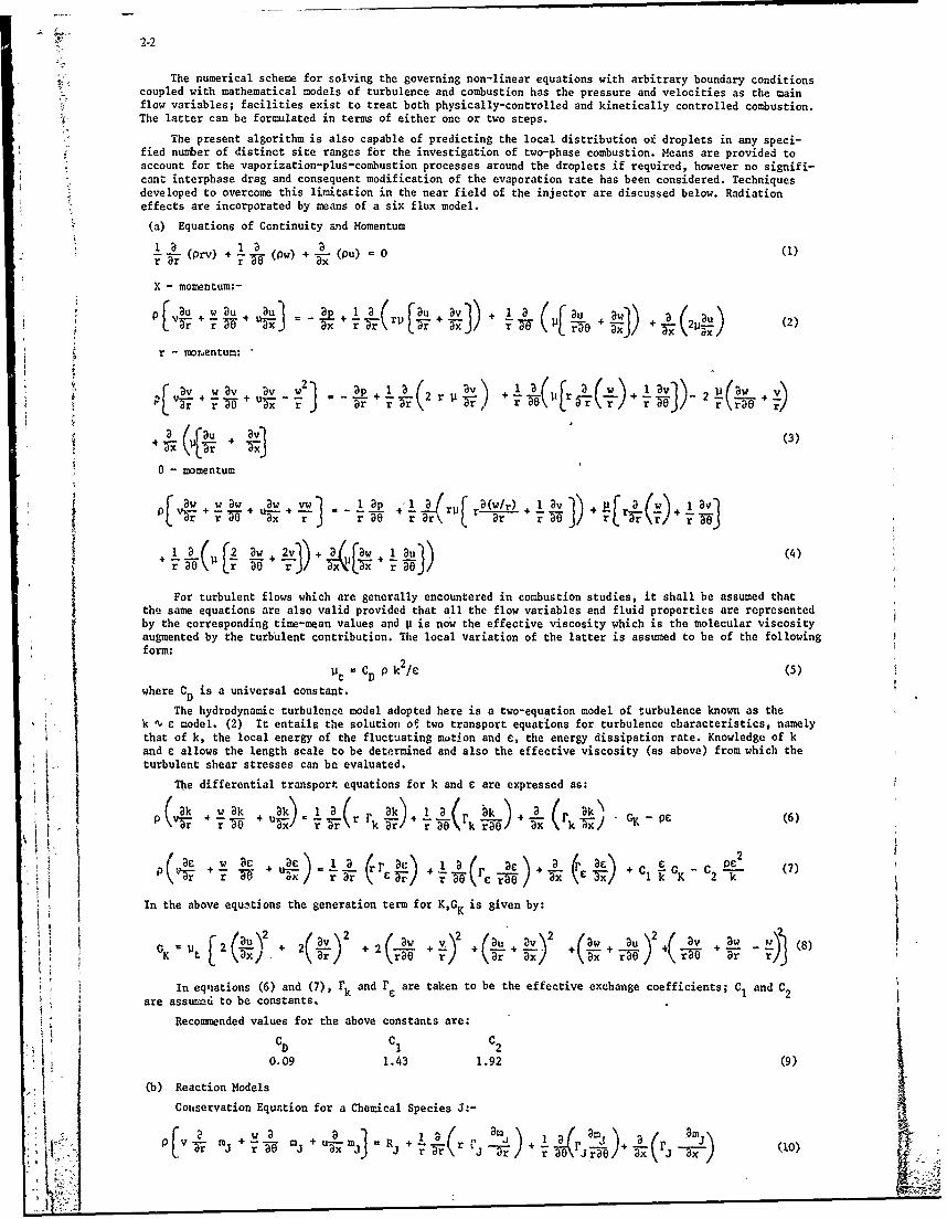
The numerical scheme for solving the governing non-linear equations with arbitrary boundary conditionscoupled with mathematical models of turbulence and combustion has the pressure and velocities as the mainflow variables; facilities exist to treat both physically-controlled and kinetically controlled combustion.The latter can be formulated in terms of either one or two steps.

The present algorithm is also capable of predicting the local distribution of droplets in any speci-fied number of distinct site ranges fbr the investigation of two-phase combustion. Means are provided toaccount for the vaporization-plus-combustion processes around the droplets if required, however no signifi-cant interphase drag and consequent modification of the evaporation rate has been considered. Techniquesdeveloped to overcome this limitation in the near field of the injector are discussed below. Radiationeffects are incorporated by means of a six flux model.

(a) Equations of Continuity and Momentum

? F(Prv) "+ (- w) + (Pu) = 0 (I)

X - momentum:-

+) + I + ) + (. (2)

r - mor.entum:

-v w av Bv 2 !W_ +

S 1 + x - r- -(3)

8 - momentum

([ 3w ww a. w +vw ap +1 rp Bw/r) + 1 v +R[ a()+I

[2 ar .v)+x [ 1uJ) (4)

30~3 To r r

For turbulent flows which are generally encountered in combustion studies, it shall be assumed thatthe same equations are also valid provided that all the flow variables and fluid properties are representedby the corresponding time-mean values and V is now the effective viscosity which is the molecular viscosityaugmented by the turbulent contribution. The local variation of the latter is assumed to be of the followingform:

Ut . CD p k21/ (5)

where CD is a universal constant.

The hydrodynamic turbulence model adopted here is a two-equation model of turbulence known as thek 1v c model. (2) It entails the solution o two transport equations for turbulence characteristics, namelythat of k, the local energy of the fluctuating motion and c, the energy dissipation rate. Knowledge of kand c allows the length scale to be determined and also the effective viscosity (as above) from which theturbulent shear stresses can be evaluated.

The differential transport equations for k and e are expressed as:k w ak k ) + f) a I ak ) (P\ r r? x 1 - 1FFrr r3O 3-k % (6)

Lk) +u~ .A -L(' - r (6)-Dr rDO T r ar k r 30 3 6 (x kc 3(3 ) 2Y P

r(B +M er C c (C 7x ' ClktK 2kpV~r +r Y-O r ua- FTr +=r r To a x a c k - C2"k 7

In the above equ..tions the generation term for K,GK is given by:

Lu+2( +2-+- M" v ~ ~ +-8a r / raO r/\ Dr 3x0 a3x 're- 7 r

In eq'uations (6) and (7), rk and r are taken to be the effective exchange coefficients; Cl and C2are ass"u"~d to be constants. 2

Recommended values for the above constants are:

CD C1 C20.09 1.43 1.92 (9)

(b) Reaction Models

Conservation Equation for a Chemical Species 3:-

P [r-? 0 m. u a-m. ,Rj + 1 a (r VJ , ( am TD + r (10)rP rBO r r T iJr rB1J ax~~I LJ7I

AZ

2-3

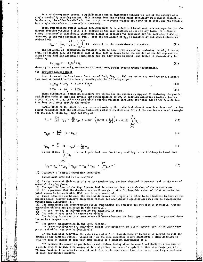
In a multi-component system, simplifications can be introduced through the use of the concept of asimple chemically reacting system. This assumes fuel and oxidant react chemically in a unique proportion.Furthermore, the effective diffusivities of all the chemical species are taken to be equal and *he reactionis a single step with no intermediate compounds.

These supposirions enable various concentrations to be determined by solving only one equation for themixture fraction vuriable f (Fig. 1.), defined as the mass fraction of f'iel in any form, for diffusionflames. Treatment of kinetically influenced flames is affected via equations for the variables f and mfu,where mfu is the mass fraction of fuel. Thus the evaluation of m, in kinetically influenced flames isachieved via: f f

m - -f -] St where St is the stroichiometric constant. (1)[xFf u (I f s'Jt(1

The influence of turbulence on reaction rates is taken into account by employing the eddy break upmodel of Spalding (3). The reaction rate in this case is taken to be the smaller of the two expressionsgiven by the familiar Arrhenius formulation and the eddy break-up model. The latter is conveniently des-cribed as:

Rfu,EBU - CRtg /k (12)

where CR is a constant and g represents the local mean square concentration fluctuations.

(c) Two-step Kinetic ModelPredictions of the local mass fractions of fuel, C02 , CO, H20, 02 and N2 are provided by a slightly

more sophisticated kinetic scheme proceeding via the following steps:

C12 + 120 + 12CO + 12H20 (13)

12CO + 602 4 12CO2 (14)

Three differential transport equations are solved for the species f, mfu and CO employing the partialequilibrium model of Morr and Heywood for concentrations of CO. In addition algebraic equations for theatomic balance of C,H, and 0 together with a trivial relation involving the total sum of the species massfractions completely specify the problem.

Manipulation of the algebraic expressions involving the individual element mass fractions, and the in-herent assumption that the effective turbulent exchange coefficients for all the species are equal through-out the field, yield %x9 mH20 and Mn02 as:

5mox 6 168 fu + 23- 0.232 I f - 0.232 Z od J

J=l

216 (f-rnu) (16)5 1 2o 168 fu

22 44 (17)CO2 7 (f-mf) - 2 8 mCO

In the above, K is the liquid fuel mass iraction prevailing in the field.mN2 is found from

J=lmfu + CO + Kn 0 ox + mN2 Md,Sf u +mco + mco02 '11R20 + +o mN d + , 1 (18)

(d) Treatment of droplet (particle) canbustion

Assumptions involved in the analysis:

(I) In the course of diminution of size by vaporization, the heat absorbed is proportional to the mass ofmaterial changing phase.(2) The specific heat of the liquid phase fuel is taken as identical with that of the vapour-phase.(3) It is presumed that the droplets are small enough in size for Reynolds number of relative motion be-tween phases to be negligible (N.B. see later discussion).(4) Under turbulent conditions, the mode of diffusion 'for droplets is taken to be identical to that of thegaseous phase; however relative dispersion effects for near-dynamic equilibrium cases can be incorporatedwithout much difficulty (6).

(5) The temperature and concentration fields surrounding the droplets are spherically symmetric. (Forcedconvection effects are neglected in this analysis).(6) The droplets are of uniform density and spherical in shape.(7) The mode of mass transfer depends on either:

The driving force due to a temperature difference between the local gas mixture and the presumed drop-let surface temperature.or: The oxygen concentration in the local mixture.

The above restrictions are convenient rather than necessary and can be removed should the extra com-Vputational effort and cost be justifiable.

Inqa the partowicle radyis Cthoie of a ate s paraterioffers coSwhicisideralifi t iIn the following analysis, ihe size of a particle is characterised by S, which is identified with thesquare of the particle radius. Choice of S as the size parameter offers considerable simplification in

that the' rate of change of size with time emerges as a constant independent of S.IV' defines the number of particles in unit volume having sizes between S and S+dS; M is the mass of

a single droplet in this size range, while m signifies the mas of droplets in this size range per unitvolume. Finally, fj denotes the mass of particles in the size range SJ+ to a larger size Sj pc. unit mass4 'J$, of local gas-droplet mixture. '

2-4

A control volume analysis for a balance of, doplets entering, leaying and changing size together withhypotheses, about the interphase mass transfer yields the following governing equation for fj: (7).

SJ

3't, ) fd 3( 2. dS) (19)

S jsJ+l

VThis study employs the comonly used supposition that the mass transfer rate from the condensed phaseto the gaseous phase per unit surface area is expressible in the form:

m,, -iin (1+B) (20)r

For distillate fuels, B is evaluated from:

TgB =q/j CpdT -Tr fCpdt-) / L (21)

Even though the actual mws variation of a two-phase mixture can only be described by a smooth curve,it suffices for purposes of this study to discreti~e this distribution. Arrangement of the droplet sizesis in such a manner that J=l signifies the largest size and J=K the smallest. This is done for the consid-erable simplification that this arrangement offers in the linearization of the source terms. The finalequations are expressed in the following form:

d r fJ-1 f__ 3 f fd- (PfJ) - in (I+B) -2 +TF J p S -I S J S r-S3+.~~ -1% J fo J+K(22

( ) or 1 + 3 fl I for J- 1 (23)

P 1 1 2

Pp K-1 _ 3 sk for J- K (24)

tn view of the fact that the concentiation of droplets in an intermediate size range :s influencedonly by the behaviour of larger droplets, not of the smaller ones,(equations (22) to (24)), a specific drop-lets treatment can be devised. This offers extremely economical use of storage while permitting an ex-tremely sophisticated representation of the droplet size distributions. The essential feature is statedas follows:

It suffices to provide storage for just one droplet concentration array. The computation is soarranged that the integration proceeds through the droplet-size distribution from large size to small, over-wricing the contents of each concentration store as it does so. This is particularly valuable when storageis a near prohibitive factor.

The incorporation of the droplet size distribution equations and the corresponding source term mani-

pulations are discussed in great detail in Reference (7).

(e) Radiation effects

The effect of radiation in the mathematical model are accounted for, by reference to the six flux modelof radiation. The differential equations describing the variations of the fluxes are:

d f Sc-(rI) r (aS )J + aE + - (I + J + K + L + M + N) (25)

(J) r(a4S + aE -(I + K + L + + N) (26)dr L r 6 J K L H N J(6

dSe(K) --(a+S,)K + aE +TIJ K L M N

d(L) (a+Sc)L -aE- c (I

• 'd'-x .I ,6 + N (28)

r( 4) = - (- + 1 4 K + L + H + N)

~d(N) (a+ScN aE - (Ii

rd 6' (30)

The composite fluxes defined as:Ry ( + J) (31)

Rx = (K+ L) (32)

R1 2 (4 + (33

are employed to eliminate I,J,K,L,H and N fr6m the pre~ious equations to yield Lhree second-order ordinarydifferential equations.

2-5

The recent radiation model developed by Lockwood and co-workers (8) where the inherent grey gasassumption of the above formulation is relaxed by employing a pseudo-grey approximation for the localemissivity, could be used for improved radiation predictions.

(f) Solution Procedure

The previous governing partial differential equations for mass, momentum, energy, droplet and speciesare all elliptic in nature and can be conveniently presented in the general form:

div (6"t - 7, grad S) = (34)The equations are first reduced to finite difference equations by integrating over finite control

volumes (5) and then solved by a procedure described in detail in Reference (1) for three-dimensional flows.

It will be sufficientfor the purposes of this paper to summarize the pertinent features of the solu-procedure.

The numerical scheme is a semi-implicit, iterative one which starts from given initial conditions forall the variables and converges to the correct solution on the completion of a number of iterations.

Each iteration peiforms the following steps:(i) The u,v and w momentum equations are solved sequentially with guessed pressures.(ii) Since the velocities at this stage do not satisfy the continuity equation locally, a "Poisson-type"equation is derived from the continuity equation and the three linearised momentum equations. Thispressure-correction equation is then solved for corrections to the pressure field and consequent correctionsof the velocity components are established.

(iii) The "Sectional balance" (7) technique is applied to the velocity field before and after the solutionof the pressure correction equation.(iv) Thd k and e equations are then solved using the most recent values of the velocities.(v) The iteration is completed upon solution of the droplet, species concentration and all the remainingequations.

One point to note here is the implementation of the cyclic boundary condition in the 0 direction con-patible with the nature of the swirling flows.

(g) Current'physical modelling limitations and future improvements

Some of the problems facing the mathematical modeller have already been indicated above. Primarily, theflameN turbulence interaction, represented in the first part of this study by the tentative eddy break-upmodel, needs to be critically assessed, It should be emphasised that the adopted eddy break-up expressionfalls short of a probabilistic description for the temporal variation of the turbulence energy and dissi-pation, i.e. the delay time associated with the oreak-up of eddies to provide adequate interfaces with thehot gas, as a consequence of the processes initiated by the turbulence energy, seems to have been neglected.A cross-correlation analysis might be profitably adopted for this purpose.

The local Reynolds number insensitivity of the model, together with the fixed eddy states presumed inthe derivation have already been pointed out by Spalding (3). However, the latter influence can probablybe accounted by reference to a differential equation which has as the dependent variable the root mean-square fluctuation of reactedness.

The solution of a concentration fluctuation equation, especially for diffusion flaries, should beviewed as a problem of utmost urgency. The implications of employing a particular waveorm for the instant-aneous variation of the composite mass fraction needs to be explored in detail. The treatment of "unmixed-ness" for premixed flames can be developed via a similar approach.

It is the authors' belief that in predicting turbulent combusting flow situations recourse has to bemade to more fundamental approaches, initially free from all the obstructive sophistications one could en-visage. Recently there appeared in the literature a number of encouraging attempts aimed at fulfilling thistask (e.g. Ref. 9.) Chemical reactor modellng formulated in terms of a "population balance" coupled with a"mechanistic" approach to predict the gross profiles could yet initiate a new era in modern combustion re-search. It is than a relatively simple matter to introduce gradually any desired level of complexity.

Space precludes a detailed discussion of potential improvements in numerical methods. However, issues

related to gri'd bptimitation, delxneation of two and three-dimensional combustor zones, effective "restart"procedures, devising of convergence-promoting features without changing the basic structure of the algor-ithm, should be considered to achievc a computationally more "attractive" model. Further recommendationsfor improvements are to be found in Reference (7).

3. THREE-DIMENSIONAL FINITE DIFFERENCE ANALYSIS. RESULTS OF THEORY AND EXPERIMENTS

In order to assess the prediction algorithm specified above, a simple 70 mm dia. gas turbine can com-bustor shown in Fig. 2. was testedexperimentally and modelled analytically. The experimental tests werecarried out at atmospheric predsure using a total air flow rate of 0.1275 kg/s both cold and at overallair/fuel ratios of'3O and 40. The computations were carried out using the grid network of over 3000 nodesas thoih in Figs. 3 and 4, both cbld aud with overall air/fuel ratioi of 68 and 40. The flow was dividedas foll'ws: swirler 7.8% (swil No. 0.8), primary jets 25.5% (6 jets), secondary jets 29.9% (6 jets),dilution 36.8% (6 jets). Th<o'old flow computations were carried out first yielding the radial, axial andtangential velocity profiles including the recirculation Lone, as shown in Figs. 4,5 and 6. Good agreementwas 'found between the measured and predicted profiles as illustrats! in Fig. 7. Computations were thencarried out with diffusive c6mbustion using the old flow pattern to initiate the iteration procedure.This case was 3imhlated experimentally using rich premixed propane/air mixture introduced through theswirler. 'As a rolativel severe test of the mdlling, procedure, the exit turbulence levels were measured

f with a photon correlatiou laser anemometer wi h the results shoyn in Fig. 8. Again the agreement is re-kmarkably good cbnsidering the difficulty of the experiment and the complexity of the prediction, howeverthe esults suggest that the model slightly overdstimates the turbulence intensity.

7iThe mor m cplex computati6ndl procedure including the droplet spray and tzo stage kinetics was thentested, using t~teprevious results to start the iterations. In both the computaticns and experiments the

S '/ liquid fuel wa introduced as a spray of 800 included-angle from the axially located fuel nozzle. TheI ' - d roplit size distribution used for the analysis was divided, into 10 size ranges as shown in Fig. 9.

Although it would be preferable to use about 20 size increments, considerable saving in computer time is

2-6

achieved by a more modest model at this stage. The problem of representing the upper 'tail' of the sizedistribution curve is met by placing all the larger droplets in the upper size band. In practice, thesedroplets would usually impinge on the combustor wall and evaporate there as indicated in Fig. 10 (Ref. 10).The associated study reported in Ref. 9. is based on the fact, shown clearly in Fig. 11, that the flow inthe vicinity of the fuel injector is 2-dimensional even though the main combustor flow is 3-dimensional.The detailed spray trajectories can therefore be analysed in detail by the 2-dimensional computation. Itcan be seen that, for the relative initial droplet/air velocity ratios associated with conventional atom-izers, the droplets tend to travel in straight lines. In general, as a droplet becomes small enough to bedeflected by the hot gas flow, its life is zo short that it quickly vanishes. The dashed lines in Fig.lOshow that the inclusion of finite droplet heat-up time in the computations only contributes about 10% tothe droplet range. Thus, the evaporation constant B should be adjusted to compensate for the relative vel-ocity of the droplets and their actual shorter residence time in each grid cell.

The predictions of the droplet concentration distribution is shown in Fig. 12, whilst Fig 13 illus-trates the mass fraction of fuel evaporated but unburned assuming kinetic control of the reaction. Suchinformation would be invaluable to a designer concerned with quenching and the minimization of unburnedhydrocarbon formation at engine idle conditions. Our experiments indicated about 0.1% unburned hydro-carbons near the wall at the combustor exit, and were thus consistent with the predictions although de-ta'led quenching mechanisms were not modelled in this study.

When the fuel spray and two-stage kinetics are included in the model, the computation is close to thelimits of present day computers, both with regard to fast memory capacity and speed. The approach of thecomputational iteration to convergence can be monitored by the normalized error in the sum of the modulusof the mass sources as shown in Fig. 14. Although the figure shows that there is little improvement in thiserror after about 80 iterations, it was found that the temperatures and associated concentrations werestill evolving slightly even after 240 iterations. Fortunately, the trends were clearly established and itwas not economic to continue the computation to its ultimate precision. The results for exit velocity andtemperature are given in Fig. 15 and 16 respectively where it can be seen that the predicted and experiment-al values are in remarkably good agreement. The hoi exit velocity profile should be compared with the coldcase shown in Fig. 7. The true exit temperature would be slightly higher than shown, since the experimentalresult's are not corrected for radiation, and the computation would have finally converged on a slightlyhigher profile. Nevertheless, it is considered that the prediction of pattern factor would be most usefulto a combustor designer.

The predicted and measured exit concentration profiles of oxygen, CO and CO2 at an air/fuel ratio of40 are shown in Fig. 17. Again, allowing for the fact that the kinetic part of the computations have notcompletely converged the concentration profiles are in good agreement. The agreement between the measuredand predicted profiles at the exit from the primary zone is illustrated in Fig. 18, where the large radialchanges are again apparent. In the experimental studies it was found that the fuel nozzle gave a slightlyskew distribution which precluded a valid comparison of the predicted and measured circumferential vavia-tions in concentration.

The location of the highly stirred regions within the combustor may be obtained from the predictionsof the turbulence dissipation rate since mixing occurs by the movement of molecules between adjacent eddies

which simultaneously dissipates the velocity difference between the eddies. The major stirred reactor re-gions can be clearly identified on Fig. 19.

4. STIRRED REACTOR MODELLING

This second stage of the calculation consists of a procedure which represents the combustor as a net-work of interconnected stirred-and plug flow reactors and includes a detailed kinetic scheme for the chemicalspecies to be considered. A model of the fuel evaporation and mixing rate is also built into this part ofthe computation since only the fuel which has evaporated and mixed with the air can take part in the chemi-cal reaction. The objective of this stage of the computation is to quickly predict the combustion efficiencyand pollution levels produced by the particular combustor design. As with the 3-dimensional modelling, animportant aspect of the procedure is that it should be capable of predicting the trend of dependence. Forexample, it is important to be able to predict the effect which a finer fuel spray may be expected to haveon the production of nitric oxide at some particular combustor throughput.

To set up the network of stirred reactors, we require a sub-model for a well stirred reactor whichincludes the internal processes of fuel evaporation, mixing and complex chemical kinetics. In addition, tomodel the sections of the flowfield where no mixing is taking place, a plug flow reactor is required. Thiscan be achieved as a sequence of differentially small well stirred reactors or in some cases as a larger

poorly stirred reactor.

Previous stirred reactor models of combustors have been mainly confined to homogeneous combustionwith "global" reaction kinetics, and encouraging results were obtained within the limitations of thivapproach (11). Evaporation effects were later included with some success (12).

i I Although the three processes of evaporation, mixing and reaction must occur simultaneously in a com-

bustor it is convenient to consider that in a steady state condition these processes occur in series.Thisapproach allows us to calculate the reactor gaseous phase composition after evaporation and mixing havetaken place, this constitutes the homogeneous feed to the reactor, A general combustion scheme which

summarizes this is shown in Table 1. (13)

The feedstream to, or product stream from any reactor is assumed to be composed of any or all of theeight species in the above scheme. Fig. 19 shovs the composition of the general two phase steady statereactor with the liquid phase shown coalesced for convenience. Transfer from the liquid phase to the gasphase is represented by the mean fuel evaporation rate, FE.In addition it is assumad that the mean resi-dence time of each phase in the reactor is the same. This assumption is incompatible with the existence ofa relative velocity between the gas and the fuel droplets but greatly simplifies the analysis and calcu-lation of fuel distribution around any particular reactor network. It is not essential to assume this

however, and the analysis could be modified to incorporate unequal phase residence times. Transfer offluid from the unmixed state to the mixed state is assumed to take place at the- rate (mass of unmixedfluid)/TD., where iD is the characteristic turbulence dissipation timt.

Total reactor mass = i c £ (35)

2-6

achieved by a more modest model at this stage. The problem of representing the upper 'tail' of the sizedistribution curve is met by placing all the larger droplets in the upper size band. In practice, thesedroplets would usually impinge on the combustor wall and evaporate there as indicated in Fig. 10 (Ref. 10).The associated study reported in Ref. 9. is based on the fact, shown clearly in Fig. ii, that the flow inthe vicinity of the fuel injector is 2-dimensional even though the main combustor flow is 3-dimensional.The detailed spray trajectories can therefore be analysed in detail by the 2-dimensional computation. Itcan be seen that, for the relative initial droplet/air velocity ratios associated with conventional atom-izers, the droplets tend to travel in straight lines. In general, as a droplet becomes small enough to bedeflected by the hot gas flow, its life is rc short that it quickly vanishes. The dashed lines in Fig.t0show that the inclusion of finite droplet heat-up time in the computations only contributes about 10% tothe droplet range. Thus, the evaporation constant B should be adjusted, to compensate for the relative vel-ocity of the droplets and their actual shorter residence time in each grid cell.

The predictions of the droplet concentration distribution is shown in Fig. 12, whilst Fig, 13 illus-trates the mass fraction of fuel evaporated but unburned assuming kinetic control of the reaction. Such

information would be invaluable to a designer concerned with quenching and the minimization of unburnedhydrocarbon formation at engine idle conditions. Our experiments indicated about 0.1% unburned hydro-carbons near the wall at the combustor exit, and were thus consistent with the predictions although de-ta.'led quenching mechanisms were not modelled in this study.

When the fuel spray and two-stage kinetics are included in the model, the computation is close to thelimits of present day computers, both with regard to fast memory capacity and speed. The approach of thecomputational iteration to convergence can be monitored by the normalized error in the sum of the modulusof the mass sources as shown in Fig. 14. Although the figure shows that there is little improvement in thiserror after about 80 iterations, it was found that the temperatures and associated concentrations werestill evolving slightly even after 240 iterations. Fortunately, the trends were clearly established and itwas not economic to continue the computation to its ultimate precision. The results for exit velocity andtemperature are given in Fig. 15 and 16 respectively where it can be seen that othe predicted and experiment-al values are in remarkably good agreement. The hot exit velocity profile should be compared with the coldcase shown in Fig. 7. The true exit temperature would be slightly higher than shown, since the experimentalresults are not corrected for radiation, and the computation would have finally converged on a slightlyhigher profile. Nevertheless, it is considered that the prediction of pattern factor would be most usefulto a combustor designer.

The predicted and measured exit concentration profiles of oxygen, CO and CO2 at an air/fuel ratio of40 are shown in Fig. 17. Again, allowing for the fact that the kinetic part of the computations have notcompletely converged the concentration profiles are in good agreement. The agreement between the measuredand predicted profiles at the exit from the primary zone is illustrated in Fig. 18, where the large radialchanges are again apparent. In the experimental studies it was found that the fuel nozzle gave a slightlyskew distribution which precluded a valid comparison of the predicted and measured circumferential vaia-tions in concentration.

The location of the highly stirred regions within the combustor may be obtained from the predictionsof the turbulence dissipation rate since mixing occurs by the movement of molecules between adjacent eddieswhich simultaneously dissipates the velocity difference between the eddies. The major stirred reactor re-gions can be clearly identified on Fig. 19.

4. STIRRED REACTOR MODELLING

This second stage of the calculation consists of a procedure which represents the combustor as a net-work of interconnected stirred-and plug flow reactors and includes a detailed kinetic scheme for the chemicalspecies to be considered. A model of the fuel evaporation and mixing rate is also built into this part ofthe computation since only the fuel which has evaporated and mixed with the air can take part in the chemi-cal reaction. The objective of this stage of the computation is to quickly predict the combustion efficiencyand pollution levels produced by the particular combustor design. As with the 3-dimensional modelling, animportant aspect of the procedure is that it should be capable of predicting the trend of dependence. Forexample, it is important to be able to predict the effect which a finer fuel spray may be expected to haveon the production of nitric oxide at som particular combustor throughput.

To set up the isetwork of stirred reactors, we require a sub-model for a well stirred reactor whichincludes the internal processes of fuel evaporation, mixing and complex chemical kinetics. In addition, tomodel the sections of the flowfield where no mixing is taking place, a plug flow reactor is required. Thiscan be achieved as a sequence of differentially small well stirred reactors or in some cases as a largerpoorly stirred reactor.

wtPrevious stirred reactor models of combustors have been mainly confined to homogeneous combustionwith "global" reaction kinetics, and encouraging results were obtained within the limitations of thistapproach (11). Evaporation effects were later included with some success (12).

Although the three processes of evaporation, mixing and reaction must occur simultaneously in a com-bustor it is convenient to consider that in a steady state condition these processes occur in series.Thisapproach allows us to calculate the reactor gaseous phase composition after evaporation and mixing havetaken place, this constitutes the homogeneous feed to the reactor. A general combustion scheme whichsumarizes this is shown in'Teble 1. (13)

The feedstream to, or product stream from any reactor is assumed to be composed of any or all of theeight species in the above scheme. Fig. 19 shovs the composition of the general two phase steady statereactor with the liquid phase shown coalesced for convenience. Transfer from the liquid phase to the gasphase is represented by the mean fuel evaporation rate, A.In addition it is assumed that the mean resi-dence time of each phase in the reactor is the same. This assumption is incompatible with the existence of

a relative velocity between the gas and the fuel droplcts but greatly simplifies the analysis and calcu-A lation of fuel distribution around any particular reactor network. It is not essential to assume this

however, and the analysis could be modified to incorporate unequal ?hase residence times. Transfer offluid from the unmixed state to the mixed state is assumed to take place at the rate (mass of unmixed

- fluid)/cD., where -rD is the characteristic turbulence dissipation timi.

p Total reactor mass = m + c (35)

2-7

r. m/b2 C2 (36)

Using (35) Ts = V/(m2/PG + £2/P2) (37)

Gaseous phase mass balance m1 -.m2 + dm/dt (38)Liquid phase mass balance c1 - £2 - FE = d/dr39)

Mass balance on the unmi.-d fluid in the gaseous p ase

d(m u)/dt=m ;2 u u/ + FE, .. m + . m1 O -+T FE (40)u 1lm ut ut DD. ~= 'u. W' ' + iE (1' (0

dt =l u u T

dru

At the steady state = d Ddt dt

M/;2 Ts 01u(l-8) +8~Thus ml (1- +(4D)1)l,;. =Thus - E) = - a (I-) here = (42), u (43)

where TSD = T /TD (unmixedness paraneter)

Thus for a given FIE, TSD and feed conditions (43) defines the proporion of the steady state reactorgas phase which is unmixed. Therefore the reactor composition prior to reaction may be expressed asfollows:

C = u + (1- )y * (where x - f, 02 or N2 ), CS (l- )Yx u x u x 2 2 CS u CS

*N.B. w*f + + = + . * (44)

2 2 2 2

The concentrations of the unmixed species can be obtained by performing the relevant species masbalances. For example, unmixed fuel vapour mass balance is as follos:

d(m4 w) * - W(I f u ; (45)dt f ml ' f ;2 u (af + F'E (45)~~~dwf ED d,,d

At the steady state d(m u wf)/dt 0, " wf + m f + dmu f u7dt + )f dt + u"f t 0

As dwf/dt 0 0, (1-8) 'u 'f - u f + 8 - u 4)f _SD

* (1-+) t'f + )u (I-a)wf +

f- e u (1 + T SD) = 'u (1-8) + 8(46)

using (43).

The expressions for the intermediate concentrations of the mixed reactants and combustion products areobtained by performing similar mass balances on the mixod portion of the reactor gas phase.

.* f: ( (I-8)(1-' u)yf + ¢u wf TSD)/(lu)8

Using (43) and (46)

y* f u ( (1-0)(1- 'u)(I+sD)Y'f + xSD ('u(l-8)w'f + 6) (1-8) (l-'u) + rSD) (47)

Similarly:Y*x " ( (I-8)(- ' u)(I+TsD) x + TSD " u SD

Having defined the intermediate composition of the gaseous phase, i.e. after mixing and evaporation,two further balances must 'e made to determine the final reactor composition. These are the species andenergy balances for the PSR for the steady state. During the reaction siage the mixed gaseous phase concen-trarions,j*, are transformed to the final concentrationy; the unmixed gas phase concentrations,o, do notchange of course although they do contribute to the physical properties of enthalpy, specific heat anddensity.

Chemical reaction, mixed species mass balance:-m2

(i -" i)(I -u ) + Pi 0 , (48), where i 1, MT. MT total number of mixed gaseousPG'V W i i1species.

Chemical reaction, gas phase enery balarce:-

m2 Wt *m* m2 NT ,(yh-ii( - Z ci(hi - hi) u HL (9

VW. -i i 11)- + pGVWi (49)~i= 0 for adiabatic operation. NR

The species kinetic production term is given by: Pi =.1 (e. - 6.j )(F. - Bj) (50)The forwdrd and backward reaction rates are related to the reactor gas phase species concentrations by

the following:

F. . x P (f-.) y 6iWii (51), Bj - b. X. N P (- i(3 i=l i=

where X. is a third body in a dissocation reaction.MT3 n.

X = d .( (- )yi/W.), (53), The forward reaction rate constants are: f=Ae T exp (-E./RT) (54)The bcwr recin ate constants are fixed by the equilibriumi constants:-

MIT MTb. f K. Z (6.-.) (55) K. exp ( a i 6. F.0/RT) (56)3 i ji 3 1 3 1 ij lj J 1 13 1i

The system of equations is completed with the equation of state:-

2-8

Ry NT .

P P G T G RT (1-P). + RT r (57)G il u W. iT U+1 i

The final reactor gas phase composition has thui been defined and the final overall conceni :tionsmaybe expressed as:SCf = Ou wf + (1 - 011) yf (58)

and similarly for the other species.

The complete set of equations characterises a heterogeneous stirred reactor in steady state operation,they reduce to the equations for the homogeneous case if 6 is set to zero. These equations are very non-linear due to the exponential dependence of the reaction rates in temprature, additionally FE is a complexfunction of temperature and staytime, Ts , hence the WSR equations must be solved iteratively.

The technique which we have used previously is the numerical method of PSR solution developed byOsgerby (14), in which a Newton-Raphson correction procedureis employed to converge onto the solution froman initial guess. An alternative nethcd of solution due to Pratt (15) has several advantages and is nowpreferred. This method uses Newton-Raphson correction equations in terms of the ls6 variables and a self-adjusting under relaxation technique suggested by Gordon & McBride (16) which gives improved convergenceand stability. The data required for the solution are a kinetic scheme, rate data, thermodynamic data andfeed conditions. An initial guess is provided by an equilibrium calculation.

Fuel evaporation rates are obtained by numerically integrating the two simultaneous differentialequations describing single droplet evaporation and viscous drag on a droplet. The spray is assumed to con-sist of a number (usually 20) of size intervals, each of which is represented by the interval mean diameter.The spray mean evaporation rate is obtained by ifitegrating the equations over the staytime of the reactor toobtain the total fuel evaporated in the reactor and dividiug by the staytime. Initially the droplets have avelocity relative to the gas stream, however, as the drag forces acting on the droplets are inversely pro-porticnal to the diameter, the small droplets rapidly assume the local gas velocity whereas the larger drop-lets tend to retain their own -Velocity. There are two modes of combustion potssible for an evaporating fueldroplet; droplet diffusion flamef and droplet wake flames. The wake flames are generally blue due to goodmixing prior to combustion whereas diffusion flames are typically yellow due to soot formation. The velocitynecessary to cause a transition from diffusional to wake burning is a strong function of the local oxygenconcentration and falls to zero at oxygen concentrations in the range 14 - 16%, thus at such oxygen levelsa diffusion flame cannot exist. This is generally the case it. gas-turbine combustion. Using the evaporationmodel of 'ise et al. (17), we can derive the static evaporation rate:

ME = Zn (I + Bev ; where B -C (T - T )/L and X - 1.432 x 10- p(T-44.67) mTo ev(59) ev p , TL aT

To allow or the effects of droplet dynamics an empirical correlation of the type suggested byFrossling is used (18):- 2 vre1 r PG

m,F " (1 + 0.244 Re'), (60); where Re " (61)GI

In order to incorporate drag effects into the model an expression is required for the acceleration ex-

perienced by an individual droplet, the expression derived by Vincent (:9) is used:-d vr 3 C Pv 2 5

re a rel 8d 3 re where CD 0.48 + 28/Re 8 (62)dt 8 r P.D

The only information needed to al1ow calculation of the evaporation rate is the initial droplet sizedistribution and the droplet initial velocity, these are normally provided by correlations derived experi-mentally for the atomizer in use. In our studies, we use the laser diffraction drop size distributionmeter which we have developed, to characterize the spray accurately (20).

Before vaporized fuel and oxidant can react, the respective molecules must be brought into intimatecontact, the physical processes involved are termed mixing. Mixing is important under combustion conditionssince it is usually the rate determining step, however it is the most difficult process to model mathemati-cally. The principle source of mixing energy in a gas turbine combustor is the pressure loss across theturbulence generator, that is the combustion can. Since the velocity and concentration fluctuations decaysimultaneously it is proposed that the degree of mixing is equal to the degree of turbulence dissipationwithin the flow system. An energy balance is performed:

Pressure drop across baffle = Energy "held" in flow velocity profile + turbulence kinetic + dissipationenergy energy

AP/q KEav/q 3(u,/U) 2 D/q (63)It is proposed that a characteristic dissipation time TD - C*Ze/u'_ma, where C* - constant (unity),

ke = mean size of energy containing eddies (0.2Y), u'x - maximum value of the r.m.s. velocity fluctuationsBut Ts - X/5 (X =lOy) .'. TSD - 50 (u'/U)max, thus using the energy balance (62), this yields TSD = 50(P/3q)l

Thus the unmixedness parameter, TSD, used from equation (43) onwards can be related to the system geo-

metry. This parameter has high values for good mixing (> 200) and low valves (< 5) cause "blowout" due toinadequate mixing (fig. 20). A mathematical model of each process has now been described and these are com-bined using the equations derived earlier (35 4 58). The equations are solved in the following way, firstlya gas temperature is estimated so that an initial evaporation rate for the reactor can be calculated. Thenusing the above equations the homogeneous feed to a reactor can be calculated and an equilibrium calculationperformed to generate the starting values for the iterative calculation. Several iterations of the chemicalspecies equations are performed until the mass convergence test is satisfied, then the energy convergencetest is applied. If thin is not satisfied then the temperature is corrected by (H' - H)/Cp followed by re-calculation of the fuel evaporation iate and homogeneous feed condition, after which the Newton-Raphsonscheme for solving the chemical species equations is re-entered. This decoupling of the energy equation isused to avoid oscillating non-convergence caused by the non-linearity of the temperature terms. Pratt (15)suggests that a more efficient procedure is to solve the fully coupled set of equations and if oscillatingnon-convergence occurs to partially decouple the energy equation, that is, variations of temperature do notaffect the distribution of species concentrations, but concentration changes are allowed to affect thetemperature, by setting the appropriate terms in the correction equations to zero. It was found that if the

fue evportiq rte as ecacuated every time th _eperature was corrected then a slight instabilityfuel evprto o rat wavea l th te tyis introduced into the iteration, therefore the evaporation rate is only calculated for the first teniterations by which time the correction is less than 5K.

2-9

We have nou derived a method for solving an individual reactor:- we have to devise a sequence of re-actors to represent the combustor under consideration. There are several methods which can be used to de-termine these sequences:- a) Qualitative observations of combustor performance, e.g. for a typical gasturbine combustor this leads to a series model consisting essentially of a stirred reactor followed by aplug flow reactor.

% b) The distribution of "macro scale mixing", derived from theoretical and experimental tracer responsefunctions (e.g. water modelling and Argon tracer studies.) c) The distribution of 'micro mixing' energywithin the flow; in this method the stirred reactors are placed in the flow regions where high levels ofturbulence energy exist. As already discussed above, the 3-D finite difference procedure is used to deter-mine flow patterns and turbulent energy distribution and hence derive the volumes, flow rates and inter-connections of the appropriate stirred reactor network. An example of a gas turbine combustor is shownin fig. 21.

As a simple illustratior the stirred reactor network approach we will discuss its application toa novel design of "blue flawe", low pollution burner built at Sheffield (fig. 22). Air is added via aCoanda ejertor. which causes controlled recirculation of combustion products thus reducing the oxygenconcentration in the vicinity of the spray leading to wake burning. WSR1 is the main flame zone, itsvolume is set equal to that of the truncated cone bounded by the dotted line (240 cm3). The unmixednessparameter, SD, for this reactor was estimated to be 300, i.e. virtually perfect mixing. The secondaryflame zone is represented by a poorly mixed WSR2 (volume 280 cm3 ), this WSR2 was estimate,d to have TSDof 10, (fig. 22). A cooling of the recirculation flow around the narrow coanda unit annulus is to be ex-pected and vas apparent from temperature measurements carried out. Consequently a heat exchanger unit wasincorporated into the recycle path to -ake account of this (fig. 23). The kinetic scheme used for thecalculations is shown in table 2, the rate-of reaction 1 is given by

d[C 2 H2412 d 24 5.52 x 1OB . exp (-12900/T). CC]? N [02]. p-0.825 (64)dt 1? 24 2(6)

In the experimental system water was condensed in the sampling system therefore for comparison pur-poses the predicted water concentration was reduced by a factor of 10 and all other concentrations adjustedaccordingly. The initiLl droplet size distribution was described by the Rosin-Rammler expression based onour own experimental results. The spray initial velocity -as calculated using discharge coefficients basedon Tipler's results (21), assuming that all the droplets were projected with the same initial velocity.

6. RESULTS AND DISCUSSION OF THE STIRRED REACTOR ANALYSIS

The predicted values of NO and CO at the burner exit (after WSR2) are plotted against airflow rate(and hence 0) for a given set of operating conditions 'Figs. 24 and 25) together with the corresponding

experimental values. The effect of fuel pressure on NO emissions is shown in Fig. 26 and in all cases goodagreement for both trend and magnitude was obtained.

We have described a program capable of predicting thi-. performance of any sequence of reactors using adetailed evaporation model, the Tsr mixing model and a detailed chemical kimetic scheme which may be ex-tended as is necessary. However, several difficulties remain, these are mainly associated with the dataavailable rather than with the computational method. The principal problem is concerned with the chemicalkinetic schemes available. The kinetic model currently in use involves a global initiation reaction :

CHy + 02 -x CO + I H2 using the rate constant due to Edelman et al (22) eqn. (64) followed by a set

of radical reactions leading to complete reaction. This rate constant has recently been revised (Edelman6 Harsha 23) the previous value being too fast by several orders of magnitude. This approach deals wellwith the lean combustion situation but rich combustion still presents a problem as hydrocarbon fragments,radicals 4nd oxygenated species are produced and must be accounted for in the kinetic scheme. In summarythere is a need for kinetic information concerning the break-up of higher hydrocarbons (x = 10) under bothrich and lean conditions. In spite of these difficulties, on the lean side of stoichiometric the programworks well. Other areas of improvement involve refinement of the model as followsa) The evaporation model. At present, this is the Wise et al (17) model with a correction for dropletdynamic effects. Further refinements to this model based on the work of W. Sirignano (24), together withreliable data on transport properties and thermodynamic properties at the temperatures of interest for

higher hydrocarbons are the hoped for developments in this area.b) In the mixing field, studies of the interaction of reaction and turbulence and how this is related tocombustor design are needed.c) A further weakness of the stirred reactor program is that it cannot, at present, predict the forma-

tion and agglomoration of'soot. This problem can be approached from two directions. In the first, weassume that soot is an undesirable product from gas turbine combustors, and the foregoing design proceduremay therefore be used to avoid the lo~a rich conditions under which soot is formed. ;n the second, anippropriaie set of rate equations for soot fbrmation, such as those advocated by Magnussen must beused, hnd these equationr may then be incorporated into the existing computer prograw with a simple changein the input data. If the fuel to be employed ;ere residual oil or coal which burn with a more complexprocess thin simpl'e eviporation, then the appropriate module of both the computer programs would have tobe modified. H6wever, the m6dular nature of the programs and simple physical form of the variables allowsuch cianges to be made-ielati'ely easily.d) At this point, a brief discussion of the relationship between the TSD stirred reactor mixing parameterconcepts used above and the coalescence/dispersion micromixing model of Curl (26) is relevant. rurl's modelregards' the reacting mass as beingtypically made up of a large iiumber of equally sized 'eddies' behavingas small batch reactors. Eddies undergo collision from time to time and equalize concentrations when thishappens. The model does not claim to be an exact description of the processes occurring in a stirred re-actor', but predicts a decay 'in concentration of the same exponential form as that known to exist in stirreAsycItems. The general form of the equation for the rate of change of the concentration probability densityfunction p(c), is given by Pratt (27)

p(c) . a[Po(c) - p(c)] -d[c p(c)] + 88 ! p(c') p(c - c')dc' - 28 p(c) (65)

where a 1 I/(mean residence time) and 6 is one half of the fractional number of cells coalescing per second.This equatibn has normally been' solved using ,Mnte Carlo methods, however, in well stirred systems the methodof Katz et al (28) may also e used ronvehiently to compare the predictions of the coalescence/dispersion

model with those of the Vulis (29) TSD model used here. For a single stirred reactor the results are

2-10

conveniently expressed as the degree of completeness of combustion (I - 4) vs temperature and a typicalresult is shown in Fig. 27 (see Ref. 30 for further details). It is quite clear from this figure thatthe same results are obtained with either method. The TSD method has two advantages however: (a) it is

* much quicker and sipler to calculate, and (b) the asymptotic value of combustion efficiency, limited byunmixedness is simply 1/(l + I/TSD).

It may be argued that the Monte Carlo methods are more advantageous for predicting the effect of local(fluctuating) high temperatures in producing high NOx due to the high activation energy of the reaction.However, to make these predictions, the joint probabilities of the concentrations and temperatures are re-quired and these are not yet available. We must therefore judge by results, and for the situations shownin Figs 24 and 26 it appears that the method used here gives acceptable results. Indeed, if the rate con-stants for the reactions are obtained in well stirred reactors, then the errors may be self compensating.(There is a similar anomcly in the use of mean temperatures to evaluate the radiant heat flux from flames.Whilst the temperature fluctuations should exaggerate the heat flux due to averaging the non-linear T

4

term, however, it i3 well known that results acceptable for engineering purposes may be obtained neglec-ting this effect.) The value of a dimensionless time mixing parameter in assessing gas turbine com-bustor designs has beer demonstrated by Mellor (31). In the preceding discussion it is suggested thatTSD 1v /(AP/q). A related expression is given by the eddy break-up model Eq. 12, whilst Pratt (27)suggests that the local mixing intensity 8 s/k. Due to the computational simplicity of reactor networkmodelling and hence its complementary role to finite difference models, more effort is required to evaluatea mixing parameter TD (or 8) and residence time Ts(or I/a),and to define the interconnections within anetwork. It is also possible that the statistical variations in micromixed TSD between macromixed regionscould be represented by a larger number of cells in the network. This approach would then allow for thelimitations of the simple TSD model. The advantage of this approach compared to that proposed by Pratt (27)is that it eliminates the computer generated random selection procedure required by the coalescence/dis-persion approach and is therefore much more efficient in the use of computer time.

Evangelista (32) suggested an interesting experimental method of estimating the mixing intensity factor8 based on the variance of the response to a step function tracer. A new technique is presented in thenext section to determine the residence time distribution in a complex geometry. This allows the size ofeach sub-reactor and their interconnections (network) to be determined, and by a relatively simple exten-sion would also permit a micromixing intensity factor TD (or 8) to be determined for each sub-reactor.

6. IDENTIFICATION OF STIRRED REACTOR NETWORKS

Mixing in combustion systems is clearly of prime important since it is usually the rate-limiting step.It is also one of the most difficult processes to model mathematically since present day theories cannotdeal with the behaviour of individual molecules. The value of the residence time distribution (RTD) analysis,presented in this section, can be appreciated fully when use is made of such practices in the ultimate re-fining of the inherent mixing hypotheses of a finite difference formulation.

The link between the finite difference and reactor modelling consists of identifying the appropriate re-actor network from the computed flow pattern. The field distribution of turbulence dissipation obtained bythe solution of equation (7) i;j utilized to define possible stirred and p!,ug flow regions with the degreeof stirring or mixing rate being determined from the total dissipation within the reactor. Previous work bySwithenbank et al (11) can be utilized extensively in such an analysis. The finite difference part of thepredictions can also supply the local flow rates, temperatures aniinterconnections between the reactorsforming the network.

Once an appropriate reactor sequence with associated initial and boundary conditions is decided upon,the full complexity of kinetics, evaporation, mixing and other phenomena are introduced. Thus this"piecewise" approach to predicting turbulent combustion circumvents the conventional problems encounteredin physical and mathematical modelling areas and computational requirements. The overall model can besaid to share in principle, several aspects of the currently available "refined" models.

Due to our limited understanaing of the reactor network and turbulence/kinetics interactions, an ix-t perimental technique which can be applied to the complex three-dimensional flows in gas turbine combustors,I is plainly required to investigate the phenomena. Water flow visualization has been used extensively asa

qualitative method of studying the reaction zones, mixing zones and the interconnecting flows (but not atpresent, the micromixing parameter TD). Clearly this method is related to the concept of the stirred re-

actor network discussed above. One important difference between water models (or air models) and hot com-bustor flows is that the former are isothermal. If geometrical similarity is maintained and ReynoldsNumbers are chosen to ensure that the model flow is turbulent, then as a result of the well known jetsimilarity characteristics, the flow patterns in the water model and prototype will be closely related.Using "partial modelling" (33) methods in which the diameters of the holes in the combustor are increasedin proportion to the square root of the cold jet to hot chamber gas density ratio, the relative velocities

and flow patterns are even more closely modelled. 'The technique is not able to take full account of theeffect of heat release on the turbulence structure, nor the effect of the turbulent fluctuations on thelocal heat release rate. Nevertheless water (or air) modelling has proved to be an invaluable tool for thecombustor designer, and Clarke (34), for example, was able to predict quantitatively the component pressurelosses, flow distribitions and, with the introduction of a chemical tracer, the exhaust temperature profile.

Theoretical analyses by Dankwerts (35) and Zweitering (36) showed how departures from the assumptionsof perfect mixing and'ideal plug flow, could be explained in terms of distribution functions for residencetimes. Novel hypotheses about segregation, hold-up, dead-space, macro and micro-mixedness and age distri-butions were introduced and related rigorously to reactor performance.

In the present experimental studies, highly specialized identification techniques have been used toSinvestigate their applicability to gas turbine combushor design. These methods are based on correlation andgeneralized least squares parameter estimation techniques and associated diagnostic tests. In a different

context these techniqueshave been used by Cummins, Briggs anu Eykhoff (37) to estimate the dynamic systemresponse of a heat exchanger and a distillation column. Nj

The method is based on the introduction of a t-acer in a pseudo-random binary sequence of pulses. In the /.

experiments desribed below, the tracer was saturated salt solution introduced through a hyprdermic needleinto a water model of the gas turbine combustor. The response of the. system was measured by means of a

conductivity probe which could be traversed throughout the chamber. The experiments could be conducted

• 2-11I

similarly with a hot or cold combustor using tracers such as mercury vapour (38) or helium (39).Similarly,by modulating the fuel flow, (or air flow), an infra-red measurement of the CO and CO2 could be used to in-vestigate the dynamics of the kinetic processes. Since only the a.c. response signals are required, a simpleI.R. emission or absoiption signal would suffice.

The interpretation of the measurements is carried out as follows:- The output signal from a practicalsystem is almost invariably corrupted with inherent micro-mixing noise in the system. Assuming the validityof linearity, application of superposition yields:

Z(t) = y(t) + n(t) (66)where Z(t), y(t) and n(t) represent the output signal, response signal and noise respectively. The mathe-matical expression relating the process response and the applied input, i(t), is the familiar convolutionintegral, i.e.

y(t) = f hit ) i (t-t) dt I (67)

0Here h(t) is the weighting function (or impulse response) of the process.Combining equations66 and 67 the measurable output to an arbitrary input signal is given by: (inputsoccurring at times greater than Ts in the past are assumed to ha - no effect on the present output):

Ts .

Z(t) = $ h(t 1) i (t-t l ) dt 1 + n(t) (68)0

The deconvolution of the above when a short duration pulse is used yields:

Z(t) ' Klh(t) + n(t) (69)

where K1 is a constant determined by the energy in the input pulse. The approximation becomes more accurateas the pulse duration becomes shorter. A step function input yields the step response which is the integralof the impulse response. The effect of noise on the system dynamics represented by n(t) in the aboveequation can be substantially reduced via correlation techniques.

It can be shown that (40) a relationship exists between the input-output cross-corelatiuo Lunction(ccf) and the input auto-correlation function (acf), i.e.

TsRiz (T) = o h (t i ) Ri (T- tl) (t) (70)

(cf. equation 9)where Riz(r), Rii(T) and Rin(-t) represent respectively the input-output ccf, input acf and the input-noiseccf. Assuming Rii(r) can be represented by a delta function for random inputs, equation (70) reduces to thefollowing simple form:

Riz (T)= h(t)

The practical implementationof a random signal as used in system analysis and identification is apseudo-random binary signal, PRBS.

The PRBS approximates to atruly random signal due to the properties of its acf. For a periodic PRBS,this can be shown to comprise a series of triangular spikes of width 2 t where t denotes the bit interval.Furthermore, due to its constant spectral density the PRBS is persistently exciting - a desired quality ofthe input signal for parameter estimation and identification studies, as the variance of the estimatedsystem parameters is generally proportional to the inverse of the power input.

Amongst the generally available identification techniques including correlation methods, instrumentalvariables, maximum likelihood, etc, the generalised least square, GLS, algorithm has proven to be statist-ically sufficient and is linear in its formulation. The algorithm can provide unbiased estinates, a de-sirable feature, as data acquired for the formulation of simple dynamic models is almost always corruptedwith correlated noise and the need to evaluate unbiased estimates of the process model and of the noisebecomes apparent. Additionally, means exist to apply various diagnostic checks.

The algorithm is applied to discrete input/cutput data sequences it, Zt (t=l ..... N) to produce op-timal models of the form:~~~~~W - k B( - ) D ( - )

Z 1 + - t (72),. VP A( - 1 ) VP C(C- 1 )

where p is the number of integrations in the system and noise models. W represents the forward shiftoperator and k is tht system time delay. V is identified as the differencing operator (l-W-1) and A,B,Cand D are taken to be polynomials of the form:

-1) W-1 -n -1. - nA(W 1 + aW . ..... a W ; B(W- ) 1b. +.b W -

1 n I n (73)C(W)r l+CW + . CWm D(W) B + d. .... d Wm

In equation 72 the ralional transferm function driven by 1he uncorreTated sequence 9t comprises theentire extraneous behaviour.

Equation 72 can be re-expressed upon removal of the system intbgrations by data differencing in thefollowing convenient form: -k

AZt . 4- Bi + A t(4It is worth noting that unless ADC- a 1, the process parameter estimates will be biased. Hence the

GLS aims to transform the term ADC'lt iteratively to an uncorrelated sequence t via the following steps:i) The process parameters (ai,bi) are initially estimated by an ordinary least squares.ii) The residuals, viz, A -A

e t AZ Bit (75)

t(Adenotes estimated values)are analysed to be subsequently transformed by autoregression.

F e. _ Et

iii) The process input and output are filtered with the autoregression F to yield:

zF A (6z FZt(6IIA £ Fi t (77)

2-12

iv) iF and Z are modified by a new least squares fit to commence another iteration cycle proceeding fromstep ii. The final model is expressed in the form:

A(FZt) Ir Wk B (Fit) + t (78)The validity of the estimated process and noise models given by the GLS algorithm have to be established

by diagnostic checks for the statistical properties of the models. Currently available diagnostic algor-ithms utilize model order tests including determinant-ratio test, F-ratio test, loss furction analysis,pole-zero cancellation and tests for independence. In addition, auto-correlations c9 .he residuals andcross-correlations of the input and the residuals can be employed to reveal the adequateof the fitted model.

Tentative values for the time delay and model order can be obtained via the impulse response evaluateddirectly by cross-correlation of the input and output for white inputs, equation (69). An alternative meansof extracting the same information is to use the determinant ratio tests (41). The test is especially val-uable in that it limits the number of possible model orders and associated time delays prior :o parameterestimation if the signal to noise ratio is reasonably high.

Loss function analysis and the associated F-ratio test are employed once the process and noise modelshave been derived by the GLS algorithm. They are primarily concerned with the behaviour of the errorfunction in the neighbourhood of NO, oaken to correspond to the actual system order.

Additionally, residual manipulation in terms of acf's provides a critical assessment of the structureand order of the estimated model. The acf of the residuals is employed to yield an indication of themeasure of the whiteness of the residuals. The ccf, on the other hand establishes the statistical inde-pendence of the residuals and the process input.

The above ideas have been applied using the salt solution injection tracer technique to study the iso-thermal residence timie distributions in a water model of the Lycoming combustor with the objective ofquantifying the stirred and plug flow reactor locations. The predicted aerodynamic patterns yielded by thefinite difference procedures are utilized in conjunction with the GLS algorithm to determine the localmixing history. A detailed description of the experimental set up and the measuring environment is given in(7).

The investigation employed PRBS and step signals respectively as the system mode of excitation forparameter estimation purposes. The particular PRBS adopted comprises a period 15, bit interval 1.1 scewhich was fed to a solenoid valve introducing the tracer. A number of measuring stations, representativeof the distinct mixing zones in the combustor, were chosen for identification and parameter estimation.A typical sequence of operational steps adopted in such an analysis is summarized as follows:

A determinant ratio test was employed to limit the number of possible model orders for the range oftime delays suggested by the deconvoluted impulse response. GLS parameter estimation was then applied for

tvarying model orders and time delays. The optimum value for the latter was taken as that which minimizedthe sum of squared residuals. Typically noise model orders of 10-15 were adopted in an iterative scheme of5-10 steps. The loss function was recorded for all the different cases tried.

Diagnostic checks comprising mainly the evaluation of the acf of the residuals, ccf between the inputsequence and the residuals and pole-zero cancellation were applied for varying model orders and time delays.Parameter estimation and subsequent validation was carried out in a strict iterative manner. Finally theimpulse response function corresponding to the estimated model was computed and this was compared with theoriginal weighting sequence obtained from the cross-correlation analysis of the input/output data.

Measurements were made at locations marked on Fig.2 using both the conventional step response methodand the p.r.b.s. technique. The results obtained using step changes in salt concentration are illustratedin Fig. 28. The sharp cut off at station 2 within the primary jets is clearly demonstrated. The recicula-tion in the primary zone which behaves as a stirred reactor is illustrated by the response at stations 1,7 and 8. The time constant of the exponential decay together with the known primary flow rate of 0.075 £/sindicates an effective primary volume of 0.2 1 which is consistent with the anticipated value. Thesecondary zone response is indicated by the results at station 12. Correcting the measured time constantfor the effect of the primary zone and the additional secondary flow gives the volume of the secondarystirred reactor as 0.15 1

Turning next to the p.r.b.s technique, some of the results obtained are given as follows:-Station Location Order Time Delay aI a2 b1 b9

7 Primary 1 2 -0.5718 - - 112.9 -13 Primary 2 1 - 0.7527 -0.1171 3.157 - 116.59 Secondary 2 3 - 0.2929 - 0.2929 - 78.34 - 61.83

14 Dilution 2 4 - 0.3389 - 0.5284 - 17.14 - 112.3

The corresponding response curves (together with Station 14 integral) are shown in Fig. 29, whichrepresent the fitted value of the cross correlation functi6n. Integrating these curves gives a repre-sentation of the step response which can be used to determine the residence time distribution as dis-cussed above, however it appears that the p.r.b.s. method gives greater resolution as can be seen bycomparing the response at Station 14 with its integral. The experimentally determined cross-correlation(pulse response) at station 19 is particularly interesting since this point is on the opposite side of theaxis to the trace injector. The response at this point is therefore due to turbulent transport rather thanconvection. The fact that it is about identical to that above the axis shows the large scale of the turbu-lent transport, and this is responsible for the fact that the primary zone behaves as one large stirredreactor rather than as six small reactors. The effect of the reactor size is to increase the throughput atblow-off (i.e. large stability loop) as discussed in Ref. 11.

In principle the value of the mixing parameter a (or ID) can be crudely obtained from the location ofthe max-imum of the variance of the step Iresponse (see Ref. 27), however in well stirred systems such as

this, the location of the maximum is so close to zero that it cannot be clearly distinguished. Thischaracteristic is easily demonstrated by inserting reprejentative Values of ts-1 and 8 in Evangelista'sEquation t[<< y(G) >>max (11(8 -ts 1 ) ) f' ('(6 + t- )/2 ts- ) (79), -!'i ~ ~ ~ ~ Y ",'~ seod.motaaxynhgl stlrdytm uhsgsrrleemutr h eut

Thus, taking a residence time ts = I sec and B > 100 gives the time of the maximum variance t, < Y()> <0.04seconds. Fortunately in highly stirred-'systems such as gas turbine combustors the results areinsensitive to the exact value of rD(or 6). In fact, the combustion efficiency is more significantly influ-enced by the uniformity of the fuel distribution and the production of NOx may be -more influenced by the

2-13

joint probability distribution of concentrations and temperature (which is at present unknown), than by theexact value of TD . Since probability distributions tend towards gaussian when they depend on the combinationof several other probability distributions, almost whatever the shape of the separate distributions, it islikely that any effects of the p.d.f. on pollutant formation can be represented by a maximum of five para-llel stirred reactors (with recycle) in the model, the size and operating of each weighted according to aportion ! the gaussian curve.

If an accurate value of TD were required to determine the ultimate combustion efficiency achievableby any given combustor nmax = I/(1 +i/TSD)then it is believed that the noise term in Eq. 72 could be usedto tbtain this parameter quite accurately, however we have not yet investigated this possibility.

7. CONCLUSION

An overall modelling procedure has been described, and by comparison with experiment it has been de-monstrated that all the key physical and chemical factors controlling the behaviour of a real gas turbinecombustor were predicted with sufficient accuracy to be of engineering value. It is therefore considered.hat progress is being made in this complex and rapidly evolving subject.

8. AUKNOWLEDGEMENT

Financial support for this work has been received from the Science Research Council and U3AF grantNo. . This support is gratefully acknowledged.

NOMENCLATURE

i) Finite difference equations

a Absorption coefficient for radiation.B Driving force for mass transfer (dimensionless..

1' C2P CD Constants in the turbulence model.

C Specific heat.pCR Constant in the eddy break-up model.

E Black body emissive power.g Mean square concentration fluctuation of fuel species.GK Quantity in the generation term for k.

Hfu Heat of combustion.

I,J,K,L,M,N Radiation fluxes in the r, x and 8 directions.k Kinetic energy of turbulence.

Length scale of turbulence.L Latent heat of vapourization.

Mass fraction of a species J, mass fraction in size range J.mfu, m, mpr Mass reactions of fuel, oxygen and product respectively.

Mass transfer rate.

Rate of fuel injection per unit volume.M Mass of a single droplet.p Pressure.

QX, Qy, QZ Net radiative transfer in the coordinate directions.Rj Mass rate of creation of species J by chemical reaction.

Rx , Ry , Rz A dependent variable for radiation fluxes in the three coordinate directions.

r Distance from axis of symmetry, instantaneous drop radius.s Stoichiometric mass ratio.S Square of droplet radius.Sc Scattering coefficient for radiation.

S 4 Source term.

T Absolute temperature.

Tg Local gas phase temperature.5

Ts Droplet surface temperature.

t Time.u, v, w Velocity components in the x, r and z (or 8) direction.

v Velocity vector.x, z coordinate distances.r Diffu'sion coefficient, gas phase transport property.r Jeff Effective exchango coefficient for J.

AV Injection cell volume.£ Disnipation rate of turbulence.uViscosity.

0 Density.0 Stefan-Boltzman constant.j General dependent variable.Kinj Contribution of the injected mass to the variable

C Coordinate in the cylindrical-polar system.

ii) Stirred Reactor equationsA. Pre-exponential factor of the jth reaction.3B. Reverse reaction rate of the jth reaction.

b. Rate constant of the reverse of reaction j.

j ; B Transfer number in evaporation rate equation [C (T-T )ILIev p L

joint probability distribution of concentrations and temperature (which is at present unknown), than by theexact value of TD. Since probability distributions tend towards gaussian when they depend on the combinationof several other probability distributions, almost whatever the shape of the separate distributions, it islikely that any effects of the p.d.f. on pollutant formation can be represented by a maxir- of five para-llel stirred reactors (with recycle) in the model, the size and operating of each weighted according to aportion ! the gaussian curve,

If an accurate value of ED were required to determine the ultimate combustion efficiency achievableby any given combustor nmax = 1/(l +I/TSD)then it is believed that the noise term in Eq. 72 could be usedto cbtnin this parameter quite accurately, however we have not yet investigated this possibility.

7, CCNCLUSION

An overall modelling procedure has been described, and by comparison with experiment J" ,..i been de-monstrated that all the key physical and chemical factcrs controlling the behaviour of a reai as turbinecombustor were predicted with sufficient accuracy to be of engineering value, It is therefot, considered-hat progress is being made in this complex and rapidly evolving subject.

8. ACKNOWLEDGEMENT

Financial support for this work has been received from the Science Research Council and t3AF grantNo., . This support is gratefully acknowledged.

NOMENCLATURE

i) Finite difference equations

a Absorption coefficient for radiation.B Driving force for mass transfer (dimensionless

ci C2 , C D Constants in the turbulence model.

C Specific heat.p

CR Constant in the eddy break-up model.:

E Black body emissive power.,g Mean square concentration fluctuation of fuel spz-4es.GK Quantity in the generation term for k.

Hfu Heat of combustion.

1,J,K,L,M,N Radiation fluxes ir. the r, x and e directions.k Kinetic energy of turbulence.i Length scale of tirbulence.L Latent heat of vapourization.Mi Mass fraction of a species J, mass fraction in size range J.

m fu, mox, mpr Mass reactions of fuel, oxygen and product respectively.

in'' Mass transfer rate.

in''' Rate of fuel injection per unit volume.M Mass of a single droplet.p Pressure.

qX, Qy, QZ Net radiative transfer in the coordinate directions.Rj JMass rate of creation of species J by chemical reaction.

Rx, Ry, Rz A dependent variable for radiation fluxes in the three coordinate directions.r Distance from axis of symmetry, instantaneous drop radius,s Stoichiometric mass ratio,S Square of droplet radius.Sc Scattering coefficient for radiation.

S0 Source term.

T Atsolute temperature.T Local 6as phase temperature.

T Droplet surfs-° emperature.

t Time.u, v, w Velocity components in the x, r and z (or 0) direction.

4v Velocity vector.x, z coordinate distances.r Diffusion coefficient, gas phase transport property.rJ,ef f Effective exchange coefficient for J.

AV Injection cell volume.EDissipation rate of turbulence.1Viscosity.

Density.o Stefan-Boltzman constant.*General depeadent variable.

¢inj Contribution of the injected mass to the variable

C Coordinate in the cylindrical-polar system.

ii) StirreJ Reactor equationsA. Pre-exponential factor of the jth reaction.

Bj Reverse reaction rate of the jth reaction.

b. Rate constant of the reverse of reaction j.

BBev Transfer number in evaporation rate equation [Cp(T-TL)/L ]

' d -'Wlm~mn i I u n u n u ue

2-14

C. Overall gas phase mass fraction of ith species.

Cp Mean heat capacity of gas phase.

CD Uroplet drag coefficient.

D Dissipation energy term.d.. Third body efficiency of species i in reaction j.

(usually assumed to be 1).E. Activation energy of the jth reaction.

FE Fuel evaporation rate.F. Forward reaction rate of reaction j.3

F? Standard molar free energy of species i.1

f. Forward rate constant of reaction j..3HL Rate of enthalpy loss from the reactor.h. Specific enthalpy of species i.

.- Equilibrium constant of jth reaction.

KEav Mean kinetic energy.

MT Total number of mixed gaseous species.m Mass of reactor gas phase.NR Total number of reactions.NT Total number of gaseous species.nj Temperature exponent in modified Atrhenius equation.

P Pressure.p(c) Concentration probability density function.

Rate of production of species i by chemical reaction.

q Dynamic head.R Universal gas constant.Re Reynold's number of droplet.r Reaction rate.rL Droplet radius.

T Temperature.T Temperature of droplet surface.

U Mean velocity.u' Fluctuation velocity.

V Reactor volume.vrel Velocity relative to droplet.

W. Molecular weight of species i.

X. Third body concentration in a dissociation reaction j.j

a Reciprocal mean residence time.ai Scoichiometric coefficient of species i as a product, in reaction j.

8FEh non-dimensionalized evaporatonn rate. Mixing intensity factor.

Yi Mass fraction. of species i in reacror mixed gas phase.

6ij Stoichiomatric coefficient of spec-es i as a reactant in reaction j.C Mass of reactor liquid pnhse.

Mean thermal conductivity of gas phase.I viscosity.

p Density.Ij Index to indicate whether the third body participates.

TD Characteristic dissipation time.

Tz Reactor residence time.

TSD TIT, unmxednees parameter.

Proportion of gas phase which is unmixed.

SWi Mass fraction of species i in reactor unmixed gas phase.

SuperscriptsFeed conditions.

* Intermediate value (i.e. after mixing and evaporation).

SubscriptsI Reactor inlet.2 Reactor outlet.G Gas phase.L Liquid phase.f Fuel.N Nitrogen.2

02 Oxygen.

cs General combustion species.i Chemical species identifier.j Chemicl reaction identifier.E Evaporation.

E,F Forced evaporation.

@ .. .. i

2-IS

REFERENCESI.. Patankar, S.V. and Spalding, D.B. "A calculation procedure for heat, mass and momentum transfer inthree-dimensional parabolic flows", Int. J. Heat and Mass Transfer, 15, pp. 1787 - 1806, 1972.2. Launder, B.E. and Spalding, D.B. "The numerical computation of turbulent flows", Computer Methods inApplied Mechanics and Engineering, Vol. 3, pp. 269-289, 1974.3. Spalding D.B. "Mixing and Chemical reaction in steady confined turbulent flames", 13th (Int.) Symp-osium on Combustion, 1971.4. Gosman, A.D. and Lockwood, F.C. "Incorporation of a flux model for radiation into a finite differenceprocedure for furnace calculation", 14th (Int.) Symposium on Combustion, pp. 661-671, 1973.5. Gosman, A.D. and Pun, M.W. Lecture Notes for course entitled "Calculation of Recirculating Flows",Imperial College of Science and Technology, December, 1973.6. Edelman, R.B., Schmotolocha, S. and Slutsky, S. "Combustion of liquid hydrocarbons in v high-speedairstream", AIAA Journal, Vol. 9, No.7, 1971.7. Turan, A. "A three-dimensional mathematical model for gas turbine combustors", Ph.D. Thesis,University of Sheffield, 1978.8. Lockwood, F.C. and Shah, N.G. "An improved model for the calculation of radiation heat transfer incombustion chambers", Proceedings of ASME-AIChE National Heat Transfer Conference, 1975.9. Bray, K.N.C. "The interaction between turbulence and combustion", 17th. Symp (Intl.) cn Combustion.The Combustion Institute, Pittsburgh, 1979.10. Boysan, F. and Swithenbank, J. "Spray Evaporation in Recirculating Flow", 17th. Int. Symp. on Comb.The Combustion Institute, i979.11. Swithenbank, J.,I. Poll, D.D. Wright & M.W. Vincent, "Combustion Design Fundamentals", 14th.Combustion (Int.)Symposium, Pennsylvania, p.627, 1973.12. Poll, I., Payne, R., Swithenbank, J. and Vincent, M.W.Second International Symposium on AirBreathing Engines, Sheffield, 1974.13. Prior, D.S., "Pollutant Minimization by Blue Flame Staged Combustion", Ph.D. Thesis. SheffieldUniversity, 1976.14. Osgerby, IT., "An efficient numerical method for stirred reactor calculations", A.E.D.C. Report No.TR-72-164.15. Pratt, D.T. and Wormeck, .J., "CREK, A computer program for calculation of Combustion ReactionEquilibrium and Kinetics in laminar or turbulent flow", Washington State University, Report No.WSU-ME-TEL-76-1, March, 1976.16. Cordon S., and McBride, B., "Computer program for calculation of complex chemical equilibrium com-positions, NASA SP-273 (1971).17. Wise, H. et al, 5th. Combustion (Int.) Symposium, p.32, 1955.18. Frgssling, N. "The evaporntion of falling drops", Garlands Beitrage Zur Geophysik, 52, p.170, 1938.19. Vincent, M.W., "Fuel spryly evaporation in gas turbine combustors", Ph.D. thesis, Sheffield University,1973.20. Swithenbank, J. et al., "A laser diagnostic for the measurement of droplet and particle sizedistribution", A.I.A.A. Paper No. 76-69. Now published in "Experimental Diagnostics in Gas Phase CombustionSystems", Progress in Astrona.utics and Aeronautics, ed. B.T. Zinn, vol. 53, pp. 421, 1977.21. Tipler, W. "The measurement and significance of fuel spray momentum", Shell Technical Report No.APD 202/62M, 1962.22. Edelman, R.B. and Fortune, 0., "A quasi-global chemical kinetic model for the finite rate combustionof hydrocarbon fuels", AIAA paper 69-86, 1969.23. Edelman, R.B. and Harsha, P.T. "Some observations on turbulent mixing with chemical reactions",Progress in Astronautics and Aeronautics, vol. 58, Ed. L.A. Kennedy, pp.55, (1978).24. Sirignano, W.A., "Theory of Multicomponent Fuel Droplet Vaporization", presented at Vth InternationalSymposium on Combustion Processes, Sept. 1977, Krakow, Poland, to be published in Archives of Thermodynamicsand Combustion.25. Magn'ssen, B.F. and Hertager, B.H."On Mathematical Modelling of Turbulent Combustion with SpecialEmphasis on Soot Formation and Combustion", 16th International Symposium on Combustion, p. 719, 1977.26. Curl, R.L. A.I.Ch.E. J1. 9, 175 (1963).27. Pratt, D.T. "Mixing and Chemical Reaction in Continuous Combustion", Prog. in Energy ,nd Comb. Sci.Vol. 1. No. 2/3 (i976).28. Kaz, S., Evangelista, J.J. and Shinnar, R. "Scale-up criteria for stirred tank reactors", New York

I .,. University, City College, 1967.29. Vulis, L.A. "Thermal Regimes of Combustion",'McGraw Hill, 1961.30. Dixon, G.T., "Fundamentals of Gas Burner Design", Ph.D. Thesis, Sheffield University, 1970.31. Mellor, A.M., "Gas Turbine Engine Pollution", Progress in Energy and Comb. Sci., Vol. 1. PergamonPress, 1976.32. Evangelista, J.J., Shinnar, R.R., and Katz, S., "Effect of Imperfect Mixing on Stirred CombustionReactors", 12th. Symposium (Intl,) on, Comb. The Combustion Institute, p.901, 1969.33. Spalding, D.B. "The Art of ?artial Modelling", 9th. Symp. (Int.) on ComK. rhe Combustion Institute,p.33, 1962.34. Clarke, A,E., Gerard, A.J. and Holliday, L.A. "Some Experiences in Gas Turbine Combustion PracticeUsing Water Flow Visualization Techniques" 9th. Symp. (Intl) on Comb. The Combustion Institute, p.878 ,1962.35. Dankwerts, P.V. "The Effect of Incomplete Mixing on Homogeneous Reactions", Ch.Eng. Sci. Vol 11, 1,1959.36. Zweitering, T.N. "The Degree of Mixing in Continuous Flow Systems", Ch. Eng. Sci. Vol.11, 1, 1959.37. Eykhoff, P., (Ed.) "Identification and System Parameter Estimation", Part 1. Int. Fed, of AutomaticControl, Elsevier, 1973.38. Topps, J.E.C., "An Optical Technique for the Investigation of Flow in Gas Turbine Comb ptors", 17thSymp (Int.) on Comb. The Combustion Institute, 1978.39. Tilston, J.R. and Stoner, J.R. "An Investigation of the Internal Flow Mechanism; in a Pegasus 6Combustion Chamber Using A Gaseous Tracer Technique" NGTE Note No. NT 957, 1975.40. Lee, Y.W.,"Statistical Theory of Communication", John Wiley & Sons, 341, 1960.41. Billings, S.A., Ph.p. Thesis, Sheffield University, 1975.

J7J

2-16 7

Table 1. WSR COMBUSTION SCHEME

(1) Liquid fuel + Evaporated fuel (unmixed) EVAPORATION(2) Evaporated fuel (unmixed) + Evaporated fuel (mixed) )

Oxygen (unmixed) 4. Oxygen (mixtd) ) MIXING

Nitrogen (unmixed) + Nitrogen (mixed) )(3) Evaporated fuel (mixed) )

+ )Oxygen (mixed) 4. Combustion products CHEMICAL REACTIONOxygen (mixed) )C

+ )Nitrogen (mixed)

Table 2. Kerosine Combustion, Reaction Mechanism

Forward reaction rate dataReaction step A. E. (cal/mole) n..1 ]. .]

C12H2 4 + 6 02 12 H2 + 12 CO

CO + OH CO2 + H 0.56 x 101 2 544 0

H +02 OH + 0 0.22 x 10 8450 0

0 + H OH + H 0.18 x 10I 4480 1

OH + H2 H20 + H O.219 x 10 14 2592 0

OHf + OH H H20 + 0 0.575 x 1013 393 0

H + O + M OH + M 0.53 x 101 6 -2780 0

H + OR + M 1120 + M 0.14 x 1024 0 -2

H + F + M 1t2 + M 0.30 x10 0 0

0+0 + N 02 + 14 0.47 x 10 1 6 0 -0.28

N + 02 , NO + 0 0.64 x 10iO 3150 1

N2 + 0 2 NO + N 0.76 x 1014 38000 0

N + OR NO + H 0.32 x 1014 0 0

NN+ 0 + M N 0 O 0.162 x 1012 1601 0N2 0+ 2 14N20 + 0 NO + NO 0.458 x 1014 12130 0

N20 + 0 N2 + 02 0.381 x 1014 12130 0

N20 + H N2 + OH 0.295 x 1014 5420 0

(Backward reaction rates evaluated from equilibrium constants obtained from free energy function).

AXIAL PLANE I . 13

3VW1 t~4 + .

Og i. Masfacin Fig. 4. Cold flow radial10 ,1I --- 1--M4IXTURE FRACION4 f kALF SETW - -- - TANDENIAL VELOCITY A'AOFIE

Fig.. Mss factons 1 ~~--RADIAL VCLOCITY PROFILES

and temperature v's and tangential velocitymixture fraction. Fig. 2. 'Gas turbine combustor can. profiles. v

RADIAL PROFILEK .4 PLANE THROUGH HOLES

if G~~~ OFF EACH P DLTOI: IPRqR ISEOO OLlO

LOC0W CFMSTiOR, CAL9 e FFL S.ifCDO ARRAhOEI4LY4T 27 114 z7 2 3 4OT TOTIAL P011115

Fig. 3. Finite difference grid. -Fig. 5. Cold flow radidl velocity profiles.

2-17

- AXt PROFILEK i 4 PLANE THR0OUGH HOLES 1 0 3

6 OFF EACH WARY 40SE 4CONAY DLUTION Ii L l !., , -to I ol

4 i~ I~tli E lll!wi 15Irl3 , 3- 0 o ... .. . oi

Fig.6.Cold flow axial velocity profiles. Fig. 7. Cold flow axial exitvelocity-predicted and measured.

0i 0 I t 24 3F . 60 2 9ill6 05railery 0 A CUI*04*TAL TO TO tO TJ TO t TO TO TO TO- i12

1 346 6072 04 961C0120DROPLET CIZE RANGE.1ira

Fig.9. Droplet sizedistribution.

03 0 12 '

I, I . . . ..>

Fig.8. Exit turbulence intensity -

profile with combustion. , , ,

Fig.lO. Predicted droplet trajectories with andwithout heat-up time.

tI ll4~t*0004'0 I. 46 £ 0002 00 II 06

00-oc$ 001 0005

of 0001.- 1- , -,, 00, 005 0000

I it ...1 0000

4CLD900A6G4E

OROP.IZI, . ..... , 3

li * Illl. llRANGE .. . . 72 I _

l# '" ' 'l" "iI KIN[IIC CONTRlOL Alf . 411

S...*,, i Fig.12. Predicted droplet concentration Fig.13. Mass fraction of fuel evaporUteddistribution. but unburned.

Fig.ll.Axial and radial .2velocity distributionsin primary zone.

a) O mm downstream offull nozzle.

b) 6 n upstream ofprimary jets.

040 ', lo

L O i l K * it 0J~4L LL±LL.4 . it L i . i4 .

S , .- . Fig. 14.Mass source convergence criterion v's iteration step number.' E 00--

6.0 1340 AIR. 4060- AF A .40 0

EXPERIMENT K.2 1600 -I .oo0 -- HEORY 240 ITERATIONS S .ToHEORY 4

Jo2 ITRTO /> " .20

-ll

-40

".S -0, .q. .. '

I oil l . i iol (WdOi 0 .0%C I .... . ..00000 ITN

Fig.15. Predicted and measured 6 Boo E,exit velocity profile - EXPERIMENT

with combustion. T0E u :wus k ox ,, r ..-..20 ITERATIONS 8 Cox €Olk o

0 20

30006

FigA6. Predicted and measured exit Fig.17. Predicted and measured exittemperatuire profile with concentration profiles.combustion.

2-18

20 GSU 15

0 f,

% A0

PEDCTED A, F .0 NFig.19.General steady state well stirred reactor model.

co

/ CO2 VISI

0,0

Fg1.Predicted and measuredFg1.concentrations 20 J_ jets

downstream ofprimaryjes

AMRSINGL1E WSR COMPLETELY

STV2L1 PROIMARY SECONDARY DILUTION VPUIE Ul

T. 99 .13, . I .. 06-.'BLW Out

WS'R WSR WS At FR WSR , PFRl~jS .1' 03 O Fig.20.Effect of mixing parameter FSD on WSR

4J'0temperature. 1

FUELFig.21. Reactor network model.MANFME ICN

ZONE IONIC

EXIT

A;MIXER WSR1 FWLOEF~L FUEL INJECTOR,

MAIN FLAME SECONDARYFLfAME FEED AIRO ONITTED

ZONE ZONE Fi.22.Schematic representation of blue flame

Blu flm 21tO i' V - Io CI burner zones. 66

Fig.23. Blefaeburner stirred reactor network. 3641ct41 63

3 12 13 $011 0 00 23 313 10$01$ 00 30

0 P3(03C33 0 P310013 *6(0~l3

0 0 40$ 0 Mo '00 600 No (flowrate and dropsize) on NO.

0~6 301 I-)64

Pig.24. Predicted and measured Fig.25. Predicted and measuredNO cocnrtos CO concentrat~ions.A .4OE / 5

* ~ ~ ~ ~ ~ ~ ~ ~ ~ ~ 1 14J~Hl3.oo Fg2.o ocn

nog. IM Cmai4O 2M 20 i.8 aiton of TS nd8c mtos o te npt .RBS ipt

for computing partially stirred

reactor performance.

2-19

DISCUSSION

A.M.Mellor, US*Have you made any in situ spray drop size distribution measurements with the forward scattering apparatus? This

is actually desired for input conditions for the reacting finite difference code.

Author's ReplyUsing the laser diffraction dropsize distribution meter, we have carried out zme measurements in emulsified fuelflames and steam assisted atomizer flames, but not yet in gas turbine combustoms. The effect of ambient tempera-ture and pressure on dropsize distribution should be investigated urgently.

The input to the computations also requires the droplet velocity distribution. I would like to emphasize that mostcurrent methods of obtaining spray information yield spatial rather than temporal size distribution and it is nowbecoming important that we take account of the difference. At Sheffield we are measuring the droplet velocitiesby two techniques. In the first a modified laser doppler system is used, whilst the second employs a double flashruby laser to obtain a time lapse hologram of the spray. The diffraction pattern of the hologram yields the sprayvelocity distribution directly.

J.H.Whitelaw, UKProfessor Swithenbank said that he would prefer to have 20 droplet size ranges in his finite difference calculations.Our experience, in the Fluids Section at Imperial College, suggests that many fewer will be required with the rangeof diameters discussed in the presentation.

The phrase "all trends have been correctly predicted", used in the presentation tan be misleading to the designer.In this connection, the comparison of calculated mean velocity profiles, normalized with a centreline velocity in aconfined flow, can hide important discrepancies. The phrase is probably best avoided and the presentation ofcomparisons, by the calculating community at large, requires greater consideration of the designers' requirements.

Author's ReplyMy proposal that 20 droplet size ranges is generally satisfactory is based on spray evaporation computations whichwe carried out, (M.W.Vincent Ph.D. Thesis 1976), in which we used 6, 20 and 40 size ranges at typical gas turbinecombustor operating conditions. The results for 20 and 40 dropsizes were identical whilst that at 6 sizes showedsignificant errors.

With respect to predicted velocity profiles, I would suggest that both computational and experiemental mass balancerequirements ensure that the weighted mean values will agree. It is interesting to note in our results that the massflow distribution does not change much with heat addition and the velocity profiles largely reflect the change intemperature distribution. If this were a general trend it could be used to help speed up the, convergence of theequations.

A.Sotheran, UK

The processes which determine the various performance aspects of a combustor are known in most cases andempirical correlations are-already adequate to ensure that new designs achieve, fox instance, specification light upcharacteristics, idling efficiency... whilst NOx emissions are similarly predictable. Whilst modelling seems unlikelyto improve design techniques in these respects, at least in the short term they can instruct the designer on how toengineer new concepts like staging. There are new problems and possibilities on which present backgroundexperience is sparse or irrelevant and modelling might best concentrate on these. They include soot anal particleformation, charging'ue l rPeities and their effects, liner temperature and life prediction with increasingly arduousconditions and so oh. Models which ignore the inajoi unknowns are seriously incomplete.

Author's Reply

I disagree with your claim that current correlations are adequate for all purposes. For example, the airlines find thatlight-up reliability is far from ideal and scheduled flights are regularly delayed by light-up problems. Similarly, theidle efficiency of many engines still leaves inuch to be desired. I also expect the modelling techniques will help tooptimize staging, indeed the Very concept of staging derives from a model of the combustion process. However, Iagree that modelling techniques are not yet fully developed and my paper aimed to indicate the current state of the"science". With respect to soot and particle formation, the paper by Edelman et al. at this meeting shows howprogress is being made in deriving a sub-modelfor this process which can be readily incorporated in the overallcombustor models which were presented.

I welcome your comments on the importance of liner temperature and life. The important feature to predict isthe peak liner temperature and in most cases this is associated with non-uniformities in the spray distribution. Thereis relatively little fundamental work on theatmoization process andthe factors which affect the variability of the

•L . spray and mixture distribution and I certainly advocate more work in this area.

4A

2-20

Comment by R.B.Edeiman, USI will be talking tomorrow about the work that we are arguing in expanding the steps higher up in the mechanismsto include pyrolysis and partial oxidation particularly relevant to the question of soot formation.

C.M.Coats, UKHow sensitive are the stirred reactor models you have described to uncertainties in the assumed reaction scheme,particularly the representation of the hydrocarbon chemistry by a single global reaction.

Author's ReplyThe rate constants of the semi-global reactior are determ.ined from stirred reactor experiments so the predictionof stability loops, etc. is quite accurate. It is difficult to assess the accuracy of the assumed reaction scheme at awide range of conditions, although the results of network calculations carried out to date appear reasonablysatisfactory.

D.T.Peatt, US(I) With respect to Figure 27: of course, both solutions agree, as they are both asymptotic solutions to the

problem: however, in poorly-mixed regions, they may not agree with the actual physics, much less with theMonte Carlo solution.

(2) The statement on p.2-10,9 2, "However, to make .... are not yet available" is categorically wrong. On thecontrary, the joint PDF's of C and T are predicted; that is in fact the object of doing the calculation!

Authors ReplyI agree with these points and believe that in principle much more can be extracted from stirred reactor modellingconcepts than has been achieved to date. Much more experiemental and theoretical work is needed in this area.

D.C.Dryburgh, UKThere is a large loss of resolution when one goes from a 3-D finite difference model with about 30 000 grid points toa network of 6 or 7 well stirred or plug flow reactors. What is the advantage of using a reactor network instead ofthe detailed 3D calculation?

Author's ReplyThere are two main advantages of the reactor network approach: Firstly, it is possible to include highly complexchemical kinetic schemes which would not be possible with our present 3-D scheme.

Secondly, the computer time required for our reactor network programme is very small. Other importantadvantages of the concept are discussed in detail in Prof. Pratt's paper in this conference.

J.McGuirk, UKI would like to question your claim that the 3D numerical solution you have obtained is converged. From theresidual source variation you show in Figure 14, if the procedure is convergir.g at all, it sems to be converging to asolution with a mass source of about 2%- do you not find this disturbing? .f the finite-difference solution ought todo anything, it ought to obey overall mass conseivation.

Author'sRepiyIfis made ciar in the paper that the 3-D comlfutation Was not comutinued to ultimate convergence, nor were therelaaiti~n parameters optimized, as thii would hav consuhied an unjustified amount, of computer time. I guessit's a case of the common engineering approach of achieving 95% of the resulis with 5% of the effort.

J.P.Patureati, Fr(I) Did you accointfor iadiafion heat irdife in the WSR computer modcl?

(2) How many iterations are required (on the average) for cbnvergence of the WSR computer model?

Author's Reply,(1), Heat transferwas included in-the blue flame burner reactor network presented in the paper althoue)i i k this

case it was convective loss rather than radiation. There would be no difficulty in including a simplified zonemethod of radiative heat transfer.

(2), Theieare various iterations cairied out in the subroutines of the WSR network computation. I can bestanswer your question by saying thatthe overall computation olyrequires two or three minutes on amedium size computer,

2-21

H.Wilhelmi, GeThe equations for the computation or modelling of combustors became more and more complicated in the courseof the years, as there is a tendency to include additional parameters. It was mentioned in the presentati.n of thepaper that the time required for the solution of the procedure described is about six hours on a high speed computer.How is this in accordance with the statement that it will be possible in the near future to perform the same calcula-tions on a minicomputer without any simplifying assumptions in the basic equations but merely using convergencepromoting features, grid optimisation etc.

Author's ReplyThe possibility stems from the fact that whilst bulk storage (e.g. a disc) is necessary for the large number of variablesinvolved, with appropriate manipulations only a small number are actually required in "core" for computation atany one time. In spite of the fact that the full computation would require a relatively lung time on a mini-computerwith (FPP) the situation would be preferable to that at present where, at Sheffield, we can only obtain one turn-around per week on a larger machine.

With respect to future developments, the problem of the slow "diffusion of infonnlation" across a fine grid canprobably be solved by the super-position of coarser grids (the multi-grid approach). This would give about a threefold increase in speed. A further factor of about two could emerge from the hybrid grid technique. Theoptimization of the relaxation parameters could give a further two-fold increase in speed. The use of logarithmicvalues of the concentration should make the composition equations more linear and further speed-up the conver-gence. I therefore see about an n rder of ntgnitude increase in speed in the longer term.

4I- I

I.

ill

4-I

mathematical Modelling of Cas-Tuxbine Combustion Charuers

W.P. Jones and J.J. McGuirk

Department of Chemical Egineering and Chenical TechnologyIt Mrperial College

Icnn SW 7

A mathenatical model for predicting the pertorrance of gas turbine cambustion chambers is described.The model is based on the finite difference solution of the averaged form of the governing partialdifferential conservation equations and turbulent transport is apprcvirated via a variable density fomof the k-s turbulence model. The reactions associated with heat release are assumed sufficiently fastfor diemical equilibrium to prevail on an instantaneous basis; and the influence of local turbulentfluctuations in mixture strength accounted for by a $-probability density function. Liquid fuel spraysare represented by a transport equatin Zor the probability density function describing the variation ofdroplet mass fraction with droplet radius. Caiptations of 2-d axisymmetric and 3-d flows are cGparewith experimental results and an assesmrent made of the adequacy of the various submodels erbodied in theprediction procedure.

The majority of gas turbine combustion charber designs in current use have evolved over many years oflargelyempixical development. Whilst this approach has been relatively successful in the past, currentinterest and legislation concerning the reduction of ccubustion generated pollutant emissions has imposedadditional constraints, so that large departures from conventional design practice are becoming necessary.In this case existing conventional design information is of restricted value and the development of lowemission carbustion chambers is thus an expensive and tzi-consuming process. In fact it is uniTkely thatthe necessary reductions in pollutant emission levels can be achieved by purely traditional methods whileat the sare tire maintaining the no less ikortant requirements concerning such features as re-light,stability, coibustor exit teeperature pattern and durability; .a more fuxrhomntal approach is needed. Insuch circumstances the contributions which could be made by theoretical procedures for predicting combustorperformance are potentially substantial. The provision of such prediction procedures represents an areaof great current interest and is the subject of the present paper.

PRI1 ,'JS WORKMathematical models for predicting combustion chamber performance can be considered in general term

to fall within two groups: methods based on a nodular approach and those based on finite difference solutionof the appropriate partial differential conservation equations. The primary objective of the formerapproach is in most cases the prediction of pollutant emnision levels whereas in the latter wider objectivesmay be considered (e.g. prediction of outlet temperature profiles). In the modular approach spatialvariations in dependent variables such as velocityand temperature are largely ignored and no attenpt ismade at calculating the local detailed features, of the flow and reaction, except insofar as complex kineticschemes may be included. Instead the combustor is divided up into a numer of regions each of which ismodelled globally using stirred and plug flow reactor concepts. Exhaustive reviews of such methods havealready been provided elsewhere, Mellor (1 & 2), and we will concern ourselves here only with their generalfeatures, by way of illustration of which we may consider one of the more sophisticated models, namely thatdescribed by Fletcher, Siegel and Battress (3) and Fletcher and Heywood (4). In this nodel the cmbustorprimary zone is modelled by a partially stirred reactor with assumed AFR and residence time distributionsand 'unmixedness' described via a single mixing parameter; the value of which must be assigned. Thepriraryo zone is folld by a one-dirensional plug flowi reactor in which dilution air on entry is assumedto instantaneously distribute itself' across the cambustor. Thus in adlition to the essential arbitrarinessInvlved' in assi ing the various reator v01uiaS and residence times, for any particular combustion chamber,a value of the mi~hg j eter mast b6 chosen. e r del parameters depend strongly on the geometric andother details bf the paticular cmbustor being considered. They are ifvariable chosen so as to reproduce

d ssion quantty wch the is capabe of predicting. It should beappreciated that the above features .are u peculiar to the o~mdel of Fletcher et al; the deficiencies arecqmm to all reactor fetwork models. In pratice the use of such nodels appears to be restricted tointerpolation along the operating curve of 'individual crrbustors for which some sasured pollutant emissionlevel data is available and which can be used as a basis for slecting the msodel parameters. Even in thiscase it is often not possible to use fixed iodel paraaters if it is desired to encompass conditions fromidle to full power. e.g. see 1Mllor (5).

An alternative and much =ore powerful approach is that based on use and fin!.l e difference solution ofthe averaged form of the patial diffeietial conservation equations for momentum, mass, chemical speciesand energy. This appiroach is h0 ealso not without its difficulties as in the averaging process inform-ation is los so that the rsultig equations are not closed. Approimations ust be introduced for unknownterms repi ting turbufent 'diffusive' tiranspot and the ensemble averaged values of net formation rate ofthe various species befoi solution is possible. Hewever in' contrast to modular approaches approximationshave to be introduced at a much nore'fundaetal and soundly bas physical level. In the cor-servationequation approach apprximation is, intr6duced to relate well defined physical (i.e. directly measurable)quantites whereas in ouar appraes te ndel parameters invariably relate somewhat nebulous and illdefined global quantities, e.g. reactor mixedness. Wilst requiring a large computer the provision ofcalculation methods for practical ccmbustion systems based on finite difference solution of the 3-dizensional

- 4-2

forms of the conservation equations has- in the past few years become viable. An assessment of theappropriate models required is given, for exanple, by Jcnes and Whitelaw (6) and Bray (7) and theapproach has been used to predir- the flow and cmbustion in gas turbine combustors by Jones et al (8),

SSerag-Eldin and Spalding (9), .Reynolds et al (10) and Jones and Priddin (11). The approaches aregenerally similar with some not inconsequential differences occurring in the modelling of reaction.Such techniques are beginning to be used as design aids by industry and in our view are the only onesprofitable to pursue.

Same authors have attempted to combine reactor models with finite difference flow solutions. Forexample, Msier, Roberts and Henderson (12) modelled the orabustor primary zone recirculation with a wellstirred reactor and the remaining flow region was approximated by a set of reacting co-annular one-dimensional stream tubes which exchange mmentun, mass and energy. Such modelling implies that thecombustor flow (excepting the primary zone recirculationI is two-dimensional with a preferred flowdirection and no recirculation. Clearly whether or not this is an acceptable approximation will dependon the particular combustor A.eing considered. However n our view the mass and velocity of air enteringthe combustor through dilution holes will in the vast majority of designs be sufficiently large to ensurethat the ccirt ltor flow is three-dimensional and elliptic, i.e. downstream influences make themselves feltupstream over most of the combustor. Perhaps the most sophisticated attempt to combine reactor networkmodels ane0 finite difference solutions is that of Swithenbank, Turan and Felton (13). A computer codeand preditior m._thod developed by Spalding and co-workers was used to obtain a full three-dimensionalsolution to te vel-acity and temperature 'fields within the combustor, albeit with a combustion model makingno allowance for fluctuations in mixture fraction. The velocity and turbulent solutions werd then usedto select tle volumes and distribution of the various interconnected stirred and plug flow reactors. These!ection of the reactor network is now less arbitrary than in a straight modular approach, though it stilldepends on a subjective interpretation of the finib difference solutions. In coron with other reactormodels, the technique allows only the calculation oi" total pollutant emission levels and the problems inassignig individual reactor parameters reain. For example Swithenbank et al modelled a low pollutioncombustor with an 5sothermal mixer followed by two well stirred reactors. These two stirred reactors wereassigned umixedness parameter values as widely separated as 300 and 10 - the basis for these values wasnot given -- and the model then used to obtain prediction of NO and 0 emission levels in quite good agreementwith measured values over a range of operating conditions. This was achieved in spite of the fact that therate constant for, the global fuel breakdown rea,.tion was too large by several orders of magnitude. Ingeneral there can.be no rational way of estimating the values of the unmixedness paraveters and they will inany case vary fron combustor to combustor =n also with the precise reactor network chosen. Thus in thecase of, say; a new or novel cmbustor desiga one might well question whether one would be any better offguessing values for mixedness paraneters rather than estimating the pollutant emission levels directly aftera careful examination of the finite difference solution.

PRESMT 0tMTrh It'The purpose of the present paper is to describe the work being undertaken by the authors towards

developing a ormputational procedure for predicting combustion chamber performance. As stated above thisis based on the finite-difference solution of the averaged conservation equations governing the transport ofmass, momentbn and energy within the combustor. The carputational aspect-s of the procedure (e.g. finite-difference formulation, solution algorithms and techniques for handling irregular shaped geometries) arenot discussed here, rather enphasis is laid on describing thb physical models used to approximate theturbulent transport processes'and chemical reaction; this forms the topic of the next section. Exanples ofpredictions in two and three-dimensional flows are then presented so that same assessment may be made of themodels currently in use. Finally, the concluding section cchbtains some suggestions for possible inprove-,ments.

MMTM TICAL MDMLThe prbblems associated with devising a mathemticai model based (,n solution of the averaged forms o3

the governing transiprt equations for pract4cal comustioi systns are many and varied. In general it nybe necessary to provide models, for a large nntem r of separate but inter-related phenomena. Typicallymodels may, be reqauired 1- describe turbulent transport in variaJle density situations, to evaluate the tinm(or ensemblel ave of the net formation rate of e&-h of the chemical species being considered, andto describe radia ., net transfer, and multi-phase phenomena including the formation and consuTption ofparticulate matter including soot and liquid fuel sprays. In the case of gds turbine csibustion chambersnot all of the above ph&ncia are of equal importance. For exaiple the heat loss to the surrounds byradiatlve, heat transfer is rarely greater than 1% of the heat release by reaction and so its influence onthe b~ito flow, heat release and pollutant formation 6 cesses can be ccnsidered negligible. Of courseif the clcu6lation of ccmbustor Wall temerature is an objective then radiative heat trahsfer must beincluded, but this can be perfoimed after completion 6f the miin flow calculation. Also neglected in thepresent frmulation is the fonration and consumption of soot particles. Here imay be presumed that theamounts present, especially in the newer oi tustor designs, are sufficiently small for their neglect tointroduce little error. n principle there appears no reason why the presence of soot particles could notbe included in the formulation but, as far as the authors are aware, at the present time there does notappear to be ava ble a tia,.table scheme for describing soot formation. The determination of the reanformation rates of chemical species represents perhaps the central, and unresolved difficulty in developingprediction mathods for turbulent~reacting flows. Essentially the pxrblem arises because the fonTAtionrates are invariably highly non lin6ar functions of terperature and spees mass fractions, Ypowledge ofthe mean vali s of these latter quantities (to be obtained from, the solution of the appropriate transportequations) is insufficient to determine the mean value of formation rate. Fortunately howew the reactionsassociated with the nigh temperature oxidation of hydrocarhons usually have time scales very short comparedwith those charact/istic of the transport processesand the aspsaption of (instantaneous) chemicalequilibrium thus provides a reasonable approximation under many circumstances. Of course it canrnot be

4-3

appropriate under all circumstances. In particular the calculation of the fornation and emission levelsof pollutants such as carbon monoxide, unburnt fuel and nitric oxide all require consideration of finiterate reactions as do ignition and extinction phenomena. Nvertheless the assumpticn does allow theprediction of many of the major features of azrbustor operation. If in adition to the assuqrtion offast reaction the diffusion coefficients for all species and heat are. taken to be equal - an accurateassumption in turbulent fl6w - and the heat loss to the surrounds is negligible, then the instantaneousthermynamic state of the gas is determinable asa nonlinear function of a strictly conserved scalarvariable. All the relevant conserved scalar quantitities are linearly related and any one can be chosen:here we select a mixture fraction, f, defined as the mass fraction of fuel present both burnt and unburnt.Alternative choices would be the mass fraction of any element present or fuel-air ratio. With the fastreaction assumption described above the averaged forms of the appropriate conservation equations for highReynolds number turbulent stationary flows can be written *

Misa i=0o (1)Mass DU 0

'i

axi axi axj

Mixture fraction a; -1, a U'q" (3)

ax. X-.J )--

Fbr liquid fuelled systens the fuel droplets are described by

a = - a b 3 17 I (4)as3 Jax

where b(s)ds represents the mass fraction of droplets in the d&tplet radius range s to s + ds and whereis the rate of change of droplet radius by a process such as evaoratin. Amongst the approximationsiplied by equation (4) is the assumption that the relative velocity between the droplets and surrounding

fluid is zero. While this is unlikely to be a good approximation for large droplets any irprovements arelikely to bring with them very considerable increases in complexity.

The averaged equations (1) to (4) are the forms resulting from a dennity weighted decomposition andsubsequent averaging of the dependent variables where tildes represent density weighted averages and over-bars conventional averages. It should be noted that equations (1) to (4) are similar to their constantdensity counterparts. In contrast if conventional averaging were to be used then additional unknowncorrelations involving the fluctuating compcnent of density would appear. Furthx details of bothaveraging processes and their relative merits is given by Bilger (14), Jones and Witelaw (6) and Jones (15).

Before solution of equations (1) to (4) is possible approxmtions are necessary. The unknown ternsinvolving the fluctuating omponent of ve)ocity must be relate to known quantities as nuct the mean valuesof p and s. The models to be described in the following section are essentially those usez1 by Jones andPriddin (11) though there are here sm differences in detail.

TLWULECE MMMEEquations (2) to (4) contain turbulent fluxes of momentum and the scalar quantities f and b which are

here approximated via a version of the two equation k - c turbulence model introduced by Jones (16) andJones and Launder (27) adcast in density weighted forr..) I

4 ,Ihe density weighted Reynolds stress is obtained from .

H uu!=2/3 6l k -PTau i+ au 2 2 (5)1

i -§- x -~ T*-,

and the scalar fluxes given by

~af -v;___ 1 Ar P u~b" =.~T Db (6)

* In order to obtain the results to be described the equations were cast in a cyliiricalpolar oordinate system: for brevity they are here written ,sing Cartesian tensornotation.

4-4

The turbulent viscosity is expressed as

I, k l. 2=C k/e (7)

where k and e are the density weighted turbulence kinetic energy and dissipation rate of turbulenceenergy, the values of which are obtained frn the solution of the transport equations

p Uj k 3 I~T 3 d C 8a iax. - uli a -Xi(8)

- k j C ii -(2{x aX~x~J i a kax P ~2 xi Dxi ~2 -k

Equations (8) and (9) differ fran their constant density counterparts in that a term involving the productof the mean density and pressure gradients appears. An exact term qxprising the product of a fluctuatingdensity-velocity correlation and the mean pressure gradidnt arises in the density weighted turbulenceenergy equation. For this an approximation which can be inferred from Jones (15) has been used. A similartern has also been added to the e- equation. Strictly both terms should be multiplied by a constant oforder unity. The r=aining constants were assigned the following values, found to give good agreement ina wide range of 2D shear flows (see e.g. Launder and Spalding (25)).

C = .09 ; C1 1.44 ; C2 = 1.92 ; k.O; =1.3 and rT 0.9

OCOMBUSrION M)DEL

With the 'fast' reaction assunption outlined previously the instantaneous chanical equilibrium gascamposition, tenperature and density can in the case of gaseous fuelled systems be detemined as a non-linear function of the mixture fraction f. For hydrocarbons explicit expressions relating the species massfractions, temperature and density to f cannot be obtained and the instantaneous thenrmdynanic state wasobtained as a function of f "fran equilibrium calculations perfoned with the canputer prograie describedby Gordon and McBride (18). For cniputational convenience the results wze then curve fitted via leastsquares orthogonal polyncmials. Now at any location f will fluctuate with time and so knowledge of the meanvalue, f, is insufficient to detennine the local mean values of species mass fractin,m an tesperature ormean fluid density and it is neces.Ary to know the probability density function (p.d.f) for f (or someequivalent information). Following snjy rkers we here chose to specify a two parameter form of the p.d.f.in terms of the mean ? nnd the variance f". The former is to be obtained fran solution of equation (3)whereas f"2 is to be obtained fran

2

a U~f + 21 T48 -p (10)5xj XI T T ) rT1~

Following Spalding (19) the constant % was assigned the value 2.0.

both The p.d.f. introduced is a desity weighted quantity and the definition allows the determination ofbohdensity weighted and ccwientloual'averaged quantities:

e.g. f = (f) p(f) df

0 (1

and 17= f( p(f) dfo P

, o p(f)

where can represent any quantity uniquely related to f including species mass fraction or temperature.The mean fluid dencity can be obtained via the p.d.f. definition :-

p(1 = fi {)df4 l (12)

Various forms of the p.d.f. have in the past been proposed. A rectangular wave variatin of f Icorresponding to a double Dirac 6- funcfion p.d.f. v,-s suggested by Spalding (19) and used by Gosman andLocmod (20) and Serag-Eldin and Spalding (9). The 6-fumction form has the .attribute of simplicity ratherthan physical realism and more realistic forns have been proposed and used. In the present work we willutilise the 0-p.d.f first suggested by Richardson, Howard and Smith (21) and used by Jones and Priddin (11).

.i TyjI It can be written

i}<77!7- : j

4-5

p(f) fal1 bl O0 f 1 (13)

0

where

a =fj(V -11 b= (14) a

For liquid fuels it is envis--4ed that the fuel droplets evaporate to form gaseous fuel which on mixingwith air reacts in a similar mmg-er to that assured for gaseous fuels. However the mixture fraction fpreviously defined nowltniudes fuel present both in liquid and gas phases. In order to determine theequilibrium. Gate of the gas mixture it is thus necessary to know the mass fraction of fuel (burnt andunburnt) present in gaseous phase. In order to do this it is necessary to establish some instantaneousrelatlonship between the mass fractions present in liquid and gaseous phases. Here possibly the simplestassui'ption is made, nanealy that the ratio of mass fraction of gaseous fuel (burnt + unburnt) to the massfraction of fuel (burnt + unburnt) in both liquid and gaseous phases does not fluctuate with time. The gasphase mixture fraction can then be obtained fran

'I.- bds~f(14)

1 - f f Lds

Equations (11) and (12)now refer only to the gas phase and the mixture fraction appearing thereinrmust therefore be interpreted as the gas phase mixture fraction. This quantity is also used for theevaluation of the chemical equilibrium state.

I For two phase mixtures the total fluid density is given by

Pg9 (15)

1 - fbds + fb ds

where pg and pLare the densities of the gas and liquid phases respectively.

Finally to ccaplete the formulation, following Williams (22) the instantaneous rate of change ofdroplet size through evapratin is taken tobe given by

SL.+' La- (16)

where Pr is gas phae molecular Prandtl nixober and Ahfg is the latent heat.

The instantaneous, gas phase enthalpy hg and viscosity, vJg are then expressed as a function ofmixture fraction and equation (11) then used to evaluate the mean value, s.

COM4PUI!ATIMtAL DETAIlSThe ~lsdset 6f~ differ-ential equations outlined in tkjb previous scinhsbe ov~b iie

difference techniqjues for both two- and tr, ieninl reacling, and non-reacting problems Thefinite-difference6 fonrPlation uss eta ifrnigexcept in regions where nenfo 66nvection

-&minates diff~sivd-processes in',ich case &~nor cell differencing -is usied. 'The captational schm iscast in terim of the pinimtivb variables, _velocity and prlessu e an a ~sadcr t procedure is usedto obtain the pressure field, see e.g. Chorin (23) and'atnka and Spaldingl (24). Lack of space przevents

a ~ ~ ~ ~~A dtledecitoof the - xumry conditionis used fo±F each individual problem, but, wherever possiblethese 146e deduced Lfrom the exper~imetal maaMsureM tS. To *avoid the nikecessity of using f ine grids near wall

) boundAris the finite-difference siolitkons wdee patched onto fully turbulent local eqilibriLni wal-;-lawrofils, se ' g Launder Sid'Spalding (25). -Ifonnirkti6n on'the grid finieness and disposition is given

.! A th6 -next section foi each piocblein-discused, as, is the caiputer timet anid'itoiaga requirements where thisj i s deerred kdlevzint. The-ni~~ 'of eq"uitgns _solved'obviousl1y varier? fra probAIem to problen;, for themost omlicated case - a liquid fuelled flaiie in a 3D 6drbk;,stor - a total of 13 diffei~bntial equationsaznustbe solved, inanely : Sntinut ', 3 iraiet~bequtos 2ublence nod61 equations (k, 0), equations formean mixture fraction f and its variance f " and 5 equations to reprvesent the droplet size distribution.-These latter equations were obtained from equation, (4) by Thtegratling overa given size range s~ to s~ to4 +

4-6

obtain an equation for the mass friction of droplets within this size range. From information on thedroplet size distribution produced by the fuel injector considered, 5 size range bands were judgedsufficient.REULTS AND DISCUSSION

As an example of predictions obtained in isothermal flow in a two-dimensional model combustorgeometry, the measurenents of Owen (26) are first considered. The flow configuration consists of acentral air jet surrounded by a faster-moving co-axial annular air stream, both streams exhausting intoa circular duct of slightly larger diameter - the flow is therefore axisyinetric. At high velocityratios (annulus/jet velocity) the central air stream is rapidly entrained by the annular jet and arecirculation region is formed on the duct centre-line; a further negative velocity region is observednear the outer wall caused by the sudden exparsion of the duct radius. In Figure 1 the predictionsobtained using the too-equation k-c model are caopared with the measurenents of Owen (1975). The Figureshows the predicted and measured position of the separation streamlines which enclose the two reci.-culationregions described above for a velocity ratio of 12 ; the predictions were obtained with a fairly finegrid (40 axial x 20 radial grid nodes) and are believed to be grid indepdndent. The agreement is goodalthough both radial and axial dimensions of the central recircu-ttion are under-predicted, a featurewhich other authors have also observed in calculation of free recirculation regions with two-equationturbulence models.

Measurements have also been made of reacting flow in the same geanetry by Spadacini, Owen and Bonan(27) ; in this case the central air jet was replaced by a jet of natural gas, and thep ossibility ofintroducing swirl into the annular air stream was included. The flow field whicl results under burningconditions is shown in Figure 2 in tens of predicted and measured axial velocity contours. The velocityratio (air/fuel velocity) in this instance was 21, the over4ll equiva ence ratio 0.9, conbustor pressure3.8 atmospheres and the air and fuel. inlet terperatures 750K and 300 K respectively. Figure 2(a) shows

4 results where the air stream had zero swirl velocity and Figure 2(b) gives the predictions and measurementsfor the case where the annular air stream also entered with a swirl canponent of ve.ocity (The svirl Nofor the run considered was 0.3 (Swirl No = tangential nnentum flux/axial mnentum ..ux x effectiveannulus diameter) ). In the first case a central, spheroidal recirculation region d measured as in theisothermal flow, and Figure 2(a) shows that this is also what is predicted. Again tie size of the ceetralnegative velocity region (shown shaded) is underpredicted. In the reacting flow case the strength of thebackilow is in addition found to be too weak, the maximun negative velocities being only about half ofthose measured. Further the acceleration of the fluid along the centre-line is too sla, particularly inthe swirling flcw case. The qualitative effect of sirl is however reproduced correctly in that thecentral negative velocity region changes in shape from spheroidal to toroidal, although again its voluneand strength are underpredicted. These calculations were made with a 20 x 20 finite-difference grid, andfiner grid solutions are being btatied to ciek the results. While it is possible that the discrepanciesresult from numerical error a much more likely possibility is that the inlet conditions used (uniformaxial velocity and zero radial component in both streams) are incorrect as the data clearly indicatedsignificant intermittent penetration of the flame into the fuel injector; extension of the calculationdain upstream into the fuel jet and annular air ducts is also being investigated. Coparison of thedevelopment of the swirl velocity is shown in Figure 3 which presents profiles across the duct at threeaxial stations, the agreement is quite good in the outer half of the duct but discrepancies exist near thecentre-line at larger downstream distances. The accuracy of the exparimental data must also be questionedhowever as measurements along two radii (opern and closed symbols) show large asyrmetries.

It can be seen from the above figures that large changes in the flow pattern occur in the imnediatevicinity of the fuel injector; the measurements of tenperature and species mole fractions were alsoconcentrated in this region and Figures 4 - 7 present comparisons for the same two sets of conditions asoutlined above. Figure 4 presents predicted and measured tenperature cortours and indicates that theintroduction of swirl does not change the teperature patteni strongly from that typical of a turbulentdiffusion ilame with high teperatures occurring in the annular mixing region. Slightly highertemperatures and larger axial gradients occur in the swirling flow case and this effect is reproduced bythe predictions, although the radial gradients are much steeper in the calculations than in the data,indicating a too slow rate of mixing. The most noticeable discrepancy o-curs in the region near thecentre-line -where the predictions show the cold fuel jet penetrating far downstream whereas the data, show high teseratures very close to the injector. Amain, this is attributable to too slow mixing,

- possibly pointing to a turbulence mdel inaccuiracy; h&,6ver, the penetration of ait up into the fuel jetwould also lead to reaction and higher temperatures in this initial region, and as noted earlier, the

inlet conditions used did not allow.this. In our view this latter explanation is the more probable and,as can be seen, its ccnsequences have far reaching effects on all predicted quantities over large regionsof the flow.

The effect of swirl on unburnt hydrocarbon and CO concentration levels in the first 5 caxbstordiameters is unfortunately not predicted correctly. Once more the slow mixing is in evidence since theME contours penetrate too far~downstream; however, when swirl iq introduced (Figure 5(b) ) thc measuredreuction in itnburnt fuccxiezntation and iicrbise ii 00 16e es (see Figure 6(b) ) is not obse-ved. Ifanythii-u ociiutrs shift tream, as is l location of the high CO levels, in carplete contrastto the meatenents. T behaviour is -cosistent 4ith the predicted velocity fields for, althaigh the

c~r :influence'of-swiLrl was pricted -iiear "the inlet, qualitative discrepancies in vo-ocities wereevident iimh damtsew The reents ghow -siirl to increase the rate of recovery (of velocity)d4ni oa f wh rc ticn %fereas the predictions indicate little change. As a consequence the effectof, swlrl- t r denta hange-coeffkiien s for scalar transport is also not repxoduced. Similar dis--cep i0 bontours, althoighhere the tendenc for higher levels-to apper at the cvn-strewi ntatihstwith ihe i~rod6tibn of swirl i r ced iy the calculation. T predLcted contour mapis m~recmp~ic~ti tasu r. indicatihg relative mima along the centre line. This results from

theMmplf!ed" liriu h alss ~Us dfor" the 2D natural gas/air calculations, wihis slightly inaccurate

---The calculationofo2D-reacting flows such as that described-in the previous paragraphs is, it isbelieved; essential to the development of the mathematical r del. Only in such relatively simple gnzxmetriescan the detailed measureaents be made which are so irportant if the weak Uinks in te. mathematical model areto-be isolated; additincally, for 2D recirculating flowsh 1h possibility of obtaining fine-grid solutionsIii______N

4-7

not marred by numerical errors is feasible, whereas this is very difficult with present core-storelimitations for 3D. recirculating flows. It is still worthwhile however to apply the mathematical modelto 3D flows as useful information can be gained. The nd al described earlier is at present being appliedto the carbustor in Figure 8; at the time the calculations were performed not all details concerning thefuel injector were known, so only preliminary results are presented here. The obustor is basicallycylindrical in shape with eight rows of air holes, the first containing 4 (regularly spaced) holes andall others containing 8 holes. The symmetry properties of the geometry anant therefore that only a 90s etor had to be considered if cyclic boundary conditions were used on the two extreme circumferentialplanes. Four separate air feeds enable the air supply to each rm of holes to be calculated, and alsothat to the vaned swirler (the protrusion of the swirler into the ccvbustor was neglected). Liquidkerosene fuel was injected using a swirl ataniser which in the experiments produced a spray angle of 95owith a mean droplet d oameteof about 50 pm ; finally the oolic: air temperature was set at 5CP K andthe swirl Nuber at 0.38 (30 vane angle). The calculation was performed using a 25 x 15 x 10 grid(axial x radial x circumferential) which meant that details fo the flow through the swirler and the dilutionholes could not be resolved accurately. Coaiutational time and storage requirents were approximately28 minutes CPU time per 100 iterations and 150 K words central memory (IBM 360/195).

Figure 9 shows the predicted and measured temperature fields on a circumferential plane displaced22.5Pfrom the vertical plane of the ccmbustor as it is sketched in Figure 8 ; this plane contains neitherthe dilution air holes, nor the gaps between the swirler vanes, but these are indicated in the figure forreference purposes. In the measurements the high tenperatures in the primary zone extend right out to theliner wall, indicating complete penetration of the fuel, pro ably with impingement of some fuel droplets onthe outer wall. At present the predictions display a quite different behaviour reu.-lting from a much tooshallow spray angle; the droplets evaporate too slowly and show little spread causirg local equivalenceratios to be everywhere much richer than measured. Accordingly the temperature is everywhere too low andthe existence of fuel in the vicinity of th6 centre-line right to the exit of the ccbustor is qualitatvelyincorrect. Scme high temperatures are predicted in the outer regions interspersed with cool areas nearthe dilution air entries, but, in the initial part of the tvbustor, these are ca,=r.d Dy recirculation ofburned products from downstream between the air jets, and the observation that the fuel does not penetrateinto the outer areas remains valid. Predictions of UHC and 0) concentrations display similarly incorrectfeatures when ccmpared with measurements. The reasons for the ccmpletely incorrect spray angle are atpresent under investigation; it my be that the conditions asswmd at the injector exit are inaccurate orthat the method of inputing the spray angle is inadequate. Alternatively the assumption that the dropletsfollow the instantaneous qas velocity may be at fault - further calculations are being undertaken to isolatethe cause of error.

CONLUSIONThe paper has given a desuription of the work being undertaken towards developing a mathematical model

for gas-turbine combustion chambers based on finite-difference solution of the averaged equations governingthe transport of mass, momentum and heat. The models for approximating turbulent transport and chemicalreaction are being tested by calculating isothermal and reacting flows in 2D combustor geometries, and theapplication of the present scheme to a on. realistic 3D oonbustor is under way, although only preliminaryresults could be shcwn here; a complete report of the performance of the model in this 3D geometry will bepresented elsewhere. 7h3 predictions for the 2D gaseous-fuelled combustor indicate that the presently usedmodels are capableof calculating the flow pattern and heat release fairly well, although lack of knowle.,econcerning inlet conditions often makes definite conclusions difficult to make. Whilst this uncertainty inthe inlet conditions can account for a large part of any discrepancy between measured and predicted quantities,there are -also scme indications of a failure of the k-c turbulence noel to provide a sufficiently accuraterepresentation of turbulent transport. This is particularly so in the case of flows with swirl. If theseinlet condition and turbulence model uncertainties could be removed then a substantial improvement in theprediction of, say, the teuperature and species concentration fields would undoubtedly result. It appearslikely that the ccmbustion model used here would then be adequate as far as the calculation of major species,temperature and heat release is concernod. However, the accurate prediction of pollutant emissions willundoubtedly necessitate scne improvement in the present scheme. For example, although the primary zone COlevels are quite well predicted, ocmbustor CO emission levels under idle power conditions would certainly beIn error with the present equilibrium model. The first improvement would be to allow for the finite-rateoxidation of 0) to CO ; this will involve the inclusion of an assumed form for a two-dimensional joint pdfand the solution of additional differential equations for the mean and the variance of the C mass fraction andfor the 0 and mixture fraction covariance. Other extensions to the present model planned are to includethe prediction of nitric oxide emissions usig; the model outlined in Jones (15) and to apply the 2D calcula-tion procedure to the liquid-fuelled flames me .ured by Spaducini et al (29) in the same avi-synmetriccombustor as investigated here; this will enabi_- the droplet model to be adequately tested.

1). A.M. Mellor : Current kinetic modelling techniques for continuous flow cubustors. Proc. of Syrp.on Emissicns form Continuous Carbistion Systens, Plenum Press (1972)

2). A.M. Mellor : Gas turbine engine pollution. Prog. Energy Ccrbust. Sci. 1, 111 (1976)3). R.S. Fletcher, R.D. Siegel & E.K. Battress : The control of oxides of nitrogen enissions from

aircraft gas turbines. FAA report FAA-RD-11-2 (1971)

4). R.S. Fletcher & J.B. Heywood : A nrxlel for nitric oxide amissions fran aircraft gas turbine engines.AIDA Paper No. 71-123 (1971)

5). A.M. I.Sllor : T ubulent-curbustin interaction models for practical high intensity cubustors.XVII Symposiun (nt.) on Carinx'tion (1978)

6). W.P. Jones & J.H. Whitelaw : Coupling of turbulence and chemical reaction. Proc. of Workshop onI MVodelling of Combustion and Practical System. Los Angeles (1978)1 -7). K.N.C. Bray The interaction between turbulence and cubustion. XVII Symposium (nt.) on

• . Combustion (1978)

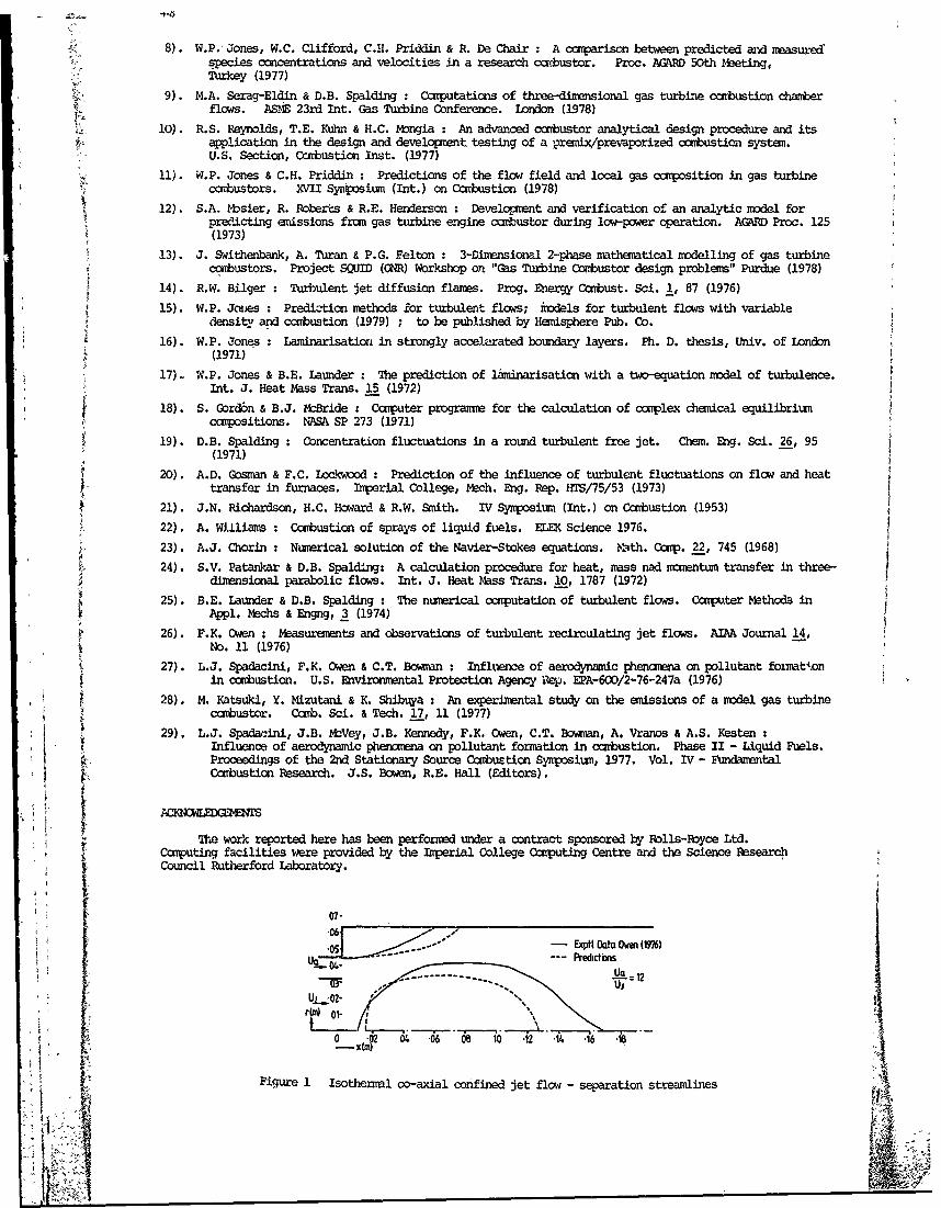
8). W.P. Jones, W.C. Clifford, C.1i. Priddin & R. Da Chair : A ccrpariscn between predicted and measuledspecies concentrations and velocities in a research ccxbustor. Proc. AGARD 50th Meeting,Turkey (1977)

9). M.A. Serag-Eldin & D.B. Spalding : Canputaticns of three-dimensional gas turbine combustion chamberflows. ASME 23rd Int. Gas Turbine Conference. London (1978)

10). R.S. Reynolds, T.E. Kuhn & H.C. Mongia : An advanced cambustor analytical design procedure and itsapplication in the design and development testing of a premix/prevaporized ombustion system.U.S. Section, Ccnibustin Inst. (1977)

11). W.P. Jones & C.H. Priddin : Predictions of the flow field and local gas caposition in gas turbinecarbustors. XVII Synjposium (Int.) on Cabustion (1978)

12). S.A. Mosier, R. Roberts & R.E. Henderson : Development and verification of an analytic model forpreOicting emissions from gas turbine engine combustor during low-power operation. AGARD Proc. 125(1973)

13). J. Swithenbank, A. Turan & P.G. Felton : 3-Dimensional 2-phase mathematical modelling of gas turbine

cambustors. Project SQUID (CR) Workshop on "Gas Turbine Cambustor design problem" Purdue (1978)14). R.W. Bilger : Turbulent jet diffusion flames. Prog. Energy Canbust. Sci. 1, 87 (1976)

15). W.P. Jones Prediction methods for turbulent flows; fidels for turbulent flows with variabledensity and ccnbustion (1979) ; to be published by Hemisphere Pub. Co.

16). W.P. Jones : Laminarisation in strongly accelerated boundary layers. Ph. D. thesis, Univ. of London(1971)

17). W.P. Jones & B.E. Launder : The prediction of laminarisation with a two-equation model of turbulence.Int. J. Heat Mass Trans. 15 (1972)

18). S. Gord6n & B.J. McBride : Ccputer programme for the calculation of complex chemical equilibriumccxrpositions. NASA SP 273 (1971)

19). D.B. Spalding : Concentration fluctuations in a round turbulent free jet. Chem. Eng. Sci. 26, 95(1971)

20). A.D. osnn & F.C. Lockwood : Prediction of the influence of turbulent fluctuations on flow and heat2 transfer in furnaces. Imperial College, Mech. Eng. Rep. HTS/75/53 (1973)21). J.N. Richardson, H.C. Howard & R.W. Smith. IV Syposium (Int.) on Combustion (1953)22). A. Williams : Cambustion of sprays of liquid fuels. ELEK Science 1976.

23). A.J. Chorin : Nuerical solution of the Navier-Stokes equations. Nhth. Coup. 22, 745 (1968)

24). S.V. Patankar & D.B. Spalding: A calculation procedure for heat, mass nad momentum transfer in three-dimensional parabolic flows. Int. J. Heat Mass Trans. 10, 1787 (1972)

25). B.E. Launder & D.B. Spalding : The numerical computation of turbulent flows. Ccmputer Methods inAppl. mchs & Engng, 3 (1974)

26). F.K. Owen : Measurements and observations of turbulent recirculating jet flows. AIAA Journal 14,No. 11 (1976)

27). L.J. Spadacini, F.K. Owen & C.T. Bowman : Influence of aerodynamic phenamena on pollutant formatonin cobustion. U.S. Environmental Protection Agency Rep. EPA-600/2-76-247a (1976)

28). M. Katsuki, Y. Mizutani & K. Shibuya : An experimental study on the emissions of a model gas turbinecombustor. Canb. Sci. & Tech. 17, 11 (1977)

29). L.J. Spadacini, J.B. MoVey, J.B. Kennedy, F.K. Owen, C.T. Bowman, A. Vranos & A.S. KestenInfluence of aerodynamic phenomena on pollutant formation in combustion. Phase II - Liquid Fuels.Proceedings of the 2nd Stationary Source Ccnbustion Symposium, 1977. Vol. IV - FundamentalCarbustion Research. J.S. Bowen, R.E. Hall (Editors).

The work reported here has been performed under a contract sponsored by Rolls-Royce Ltd.Cmputing facilities were provided by the Imperial College Computing Centre and the Science ResearchCouncil Rutherford Laboratory.

07-

-xp Dto wen (107)----:Ua 12

/,- -,,ur -ea02e

0~ 04 -06 06 10 *12 -14 *16 *18x4Figure 1 Isothermal co-axial confined jet flow - separation streamlines4

lk i.

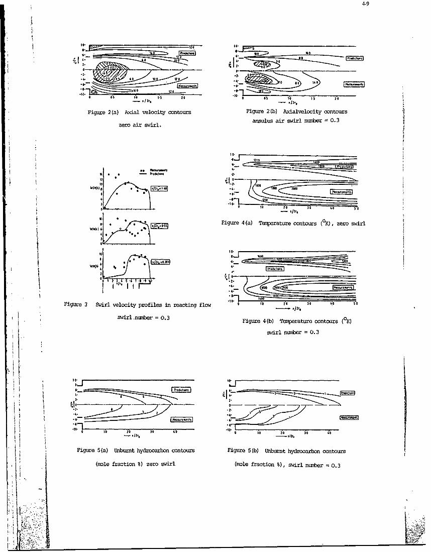
4-9

-2 6 1 *

-sso

a 04 to V$ 20 10. 0 0* 10 Is 2'0

Figuare 2 (a) Axial velocity contours Figure 2(b) Axialvelccity contours

sannulus air swirl number 0.3

Figur 4(ea)o conousi re-2(b co yntours

0 r air swr, 0.2 1 0 0 3 0 0 ,

'10 • * .,'"l'. + .Figure 4(a) Temperature contours (OK), zero swirl

Figure~ ~ ~ ~ ~ ~ ~ ~~~~~wr 3ute wilvlitprflsnretigfo " -' ,,,)0. 3 0 s

0 to 20 3o___i f

Fiur 5()wibrln yrobon ontour Figure 4(b) ratroro contours (K

S...2( in umber =3 0.3

%.- . . ..

swirl 5a) nbunhyrcro on0.3 r Figure 4(b) nbu erntrro conturs()

(mol frctio %)zer swil (olefracion),swirl number = 0.3

__ _ _ _ _ _ _ _ _ _ _ _ _ _ _ _ _ _ _ _ _ _ _ _ _ _ _ _ _ _ _ __ _ _ _ __ _ _ _ _ _ _ _ _ _ _ _ _ _ _ _ _ _ _ _ _ _ _ _ _ _ _

1f4 ° ++

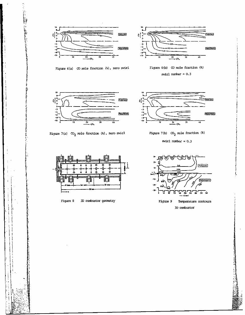
- I X - 6 : - -------__ _ _ _ _

- 00

to- ----- s4-00 10 20 i0 00 0 t0 20 30 400

Figure 6 (a) CC) mrle fraction (%), zero swirl F'igure 6(b) 00 imle fraction ()

swirl nux±ber 0.3

0to-

10o0 10 20 )o 40

Figure 7(a) C02 mle fraction (%,zero swirl Figure 7(b) O2 mle fraction M%

swirl ntiober =0.3

ji ol ~1000 06(,,I~ 1600 0-

. 16 o00 10 ~$ft0______ K w

020\

r- r-~ ~S 40 0 20 0 NO 0 24 0 3 N3016tFigure 8 3D cobustor gea1mtxy Figure 9 miperature contours

3D combustor

~~t

j-I

DISCUSSION

D.T.Pratt, USOn p.2, you overstate the case when you state "in general, there can be no rational way" etc... This is true ofFletcher and Heywood parameter which is really a standard deviation of a Gaussian (F/A) ratio distribution.

However, Swithenbank's 3 (or TSD) is easily estimated by -/AP or e/k ; the former of course from experi-mental measurement, the latter perhaps from such a model as you propose.

Author's ReplyIn our view the construction of stirred reactor models necessarily involves a very large number of essentiallyarbitrary and ad hoc assumptions related to the selection of reactor volumes, and their locations, residence time and'mixedness' parameters. At what stage the maximum uncertainty arises will in g.neral depend on the particularmodel being considered. However to turn to the 'mixedness' parameter rSD to which Professor Pratt refers I amafraid that I simply do not agree that there is a rational basis for selecting its value. Relating TSD to V/F involvesa number of what appear to be extremely dubious assumptions which, for example, take no explicit account of thesystem geometry. In any case one is still left with the problem of determining the constant of proportionality andhow one does this while still leaving something to predict is not at all clear. The alternative suggestion of relatingrSD to the local turbulence time scale k/e which could be extracted from a finite difference solution does notremove the difficulty. The turbulence time scale is a local quantity which will have different values at each spatiallocation. However for a stirred reactor model some average single value aprropriate to the total reactor volume isrequired - but how precisely is this average to be formed? This is in additon to the arbitrariness introduced viathe estimation of mean residence time.

J.H.Whitelaw, UKIt is possible that, in the comparisons which you presented the turbulence model is more at fault at a swirl numberof 0.3 than at higher or lower values? Our experience* with a swirl number of 0.23 and a similar geomety, suggeststhat there is a region of flow with swirl numbers which give rise to small regions of central recirculation, where theeddy viscosity model gives rise to more significant errors than at higher or lower swirl numbers.

*M.Habib and J.H.Whitelaw

Measured velocity characteristics of confined coaxial jets with and without swirl. To be published in J. Fluid Eng.

Author's ReplyThe experiments quoted by Professor Whitelaw certainly confirm our contention that, as in the comparisons shownin our paper for reacting flow, a two-equation turbulence model does not adequately account for the effect of swirlon the turbulent transport as the swirl number is increased from zero to an intermediate value of 0.2-0.3. Othercalculations we have performed at a higher swirl number (0.6) also indicate the same inadequacies, and, as far as weare aware, there is no evidence that the turbulence model performs any better at even higher swirl numbers.

R.B.Edelman, USDo you establish grid independence and convergence of your solution? What was the grid network you used?

Author's ReplyWe have grid independent solutions and convergent solutions in 2-D calculations. In 3-D calculations, I think it'snot generally possible to establish whether or not a good independent solution is obtained. Indeed I think it'sunlikely that you can get a true good independent solution. We used a mesh of 25 x 10 x 15. We used about ISOwords in the central memory. We did not use any secondary storage. The calculation time was 28 minutes. Goodindependent solutions in 3-D calculations are a major problem.

tI

t1L

5-I

A PREDICTION MODEL FOR TURBULENT DIFFUSION

FLAMES INCLUDING NO -FORMATION

J. JANICKALehrstuhl fUr Techn. Thermodynamik, RWTH Aachen,

D-51 Aachen, Schinkelstr. 8, GermanyW. KOLLMANN

von Karman Institute for Fluid Dynamics,Ch. de Waterloo, 72, B-1640 Rhode St Gen~se, Belgium

Abstract

A prediction model for turbulent diffusion flames burning gaseous fuels is developedand applied to H2-air flames. In the (simplified) system of chemical reactions the fastreactions are assumed in partical equilibrium wherL.3s three-body recombinations are treatedin non-equilibrium. For the H2-air flames this assumption leads to a description of thereacting system with only two variables f and r. Two methods of treating such a system ina turbulent flow are discussed : (1) modelling and solving tiansport equations for firstand second order moments of these variables and prescribing the form of the pdf of f andr as a function of the selected moments, or (2) modelling and solving the equation forthe pdf of f and r. Both sets of equations are complemented with a modified version ofthe k-c turbulence model. The NO-formation in such flames can be calculated using thenon-equilibrium values (mean valuesand covariances) of the 0 and H radicals. The resultsobtained with both models are compared with experiments and show good agreement.

LIST OF SYMBOLS

A coefficient of pdf 0 oxygen

A ,i Arrhenius coefficient P probability density function

c mass fraction p pressure

c CD''CcC2'cC3 I turbulence model P transition probability

cc4'CpuI Cpv1 'cv2 constants q a priori probability

CT'CT2 R gas constant

D nozzle diameter r reaction variable

D ,i Arrhenius coefficient Re Reynolds number

E entropy S source term

F Arrhenius coefficient Sc Schmidt number

f mixture fraction s value of r

go$i acceleration of gravity T temperature

9 variance of mixture fraction t time

H hydrogen u longitudinal velocity component

h enthalpy v velocity vector

Kc i reaction rate expression v radial velocity component

k kinetic energy of turbulence w kinetic source term

L number of statistical moments X component symbol

M inert component x Cartesian coordinate

Mi molar mass x longitudinal coordinate

m number of scalar variables y radial coordinate

N nitrogen z atomic mass fraction, value of f

n number of components in mixtureGreek symbols

a Arrhenius ixponent (forward step), flow variableexponent of beta-function S product

Arrhenius exponent (backward step),exponent of beta-function p density

y coefficient of pdf a Prandtl/Schmidt number

S6 Dirac pseudofunction p dynamic viscosity6 iKronecker symbol n statistical moment of order n

dissipation rate v kinematic viscosity

r molecular transport coefficient time scale

source term of r-equation <.> ensemble average

;p concentration

%f j_

5-2

Superscripts

o nozzle exit instantaneous

ambient u unburnt

- unweighted mean value v burnt

fluctuating part

Subscripts

b backward j component in mixture

D turbulent viscosity Z component in mixture

e equilibrium, ambient o reference value

f forward t turbulent

i component in mixture Cartesian component

J jet pipe exit S Cartesian component

1. INTRODUCTION

The prediction of the turbulent and chemically reacting flow in gas turbine combustorsis an extremely complex problem and far from a satisfactory solution. The investigationof turbulent diffusion flames is a step in gaining predictive capabilities for such com-plex phenomena. Diffusion flames contain all the important physical and chemical processesbut are structurally simpler than combustors. The mathematical treatment of turbulentdiffusion flames leads to the well-known closure problem for moment equations which isaggravated by an increased number of fluctuating field variables due to the heat releaseand different molar masses of mixture components. For this reason the complete predic-tion model is built up from : the thermo-chemical nodel describing in a reasonably sim-plified'way the instantaneous transfer of mass anJ energy, the turbulence model descri-bing the turbulent fluxes if mass, momentum and energy, the coupling model which linksthermo-chemical and turbulence modal by providing the information about the probabilitydensity function of the scalars in the thermo-chemical model that are described by dif-ferential transport equations. The pdf plays a central role in this model because it isessential for the calculation of the mean thermodynamic state of the flame at any pointof the flow field. The thermo-chemical model for H2-air diffusion flames is based on asimplified (Ref. 30) reaction mechanism for H2-combustion and assumes partial equilibriumfor fast reactions but treats the slow three-body recombinations kinetically (Ref. 5).The turbulent model is based on the k-c model of Jones and Launder (Ref. 18) and iswritten in terms of unweighted statistics. To include properly density fluctuations themodelled equations for the density-velocity correlations are added to it. For the couplingmodel two different approaches to obtain the (two-dimensional) pdf are discussed and thecomputationally most efficient method is chosen for the current prediction model. The

model is then applied to several H2 -air diffusion flames, for which experimental dataincluding NO-formation are available, to evaluate its properties.

2. THE CLOSURE MODEL

The flow in turbulent flames burning fossile fuels is extremely complex and a complete

mathematical description involves an infinite set of nonlinear partial differential equa-tions. This complexity is due to the turbulent nature of the flow and the complicated setof chemical reactions essential to the description of the instantaneous transfer of massand energy in gaseous systems. Consequently, the development of a closure model willconsist of two parts, one devoted to the thermo-chemical processes and the other to theturbulent fluxes. The link between them will be provided by the pdf of certain scalarvariables which will be constructed from a small set of statistical moments.

2.1 The thermo-chemical model

The assumptions concerning the instantaneous transfer mechanisms for mass and energyare loosely termed thermo-chemical model. The dispersion of liquid fuel in sprays and itsvaporization will not be considered here and attention will be restricted to the gaseousphase. The following assumptions are put forward : all participants in the turbulent andcombustible mixture are assumed ideal gases with possibly temperature dependent thermaland caloric coefficients. Thermal equilibrium will be assumed locally and Soret/Dufour Ieffects as well as volume forces and volume viscosity will be neglected. The moleculardiffusion in the multi-component mixture will be treated crudely by relations of the

Fick-law type. In addition, the diffusivities for all components and energy will be con-sidered equal. Radiative energy transfer will not be taken into account and the Machnumber will be significantly smaller than unity. The set of these simplifications isusually referred to as Shvab-Zeldovich assumptions (Ref. 1) and has found frequent appli-cation to the mathematical analysis of flames. For the description of the combustion ofhydrogen with air the following system of reactions is considered :

H + 02 OH + 0 (RI) H + OH + M H20 + M (R5)0 + H2 OH+ H (R2) H + 0 + M OH + M (R6) 4H2 + OH Z H20 + H (R3) 2H + M H2 + h: (R7)

20H1 H20 + 0 (114)

5-3

This mechanism was suggested by several authors (Refs. 2, 3, 4) as a reasonable descrip-tionof diffusion flame kinetics. Its range of validity was estimated (Ref. 5) in laminartest calculation and it was found to be a good approximation of the H2 -air kinetics fortemp:iritures T > 1200 K and conditions close to stoichiometric. In this range the reac-tions (R1)--(R41 are much faster than the relatively slow three-body recombination reac-tions (R-)--(R7) This leads to the hypothesis (see Refs. 2, 6) that the fast reactions(R1)-(R4) ar' in partial equilibrium. The slow reactions (R5)-(R7) are in general not inequilibrium and have to be treated by means of rate equations. In order to make efficientuse of this hypothesis combined variables are introducued according to Dixon-Lewis etal. (Ref. 2), .,i such a way that the kinetic source terms of the new variables do notcontain contributions fromthe fast reactions (R1)-(R4). They are given by

1 02 1 0 02= - - + - C0 + - - CH()02 MOH 0

2 MH

C* I Hz M H2 3 MI1

3 2H H2 (2)H2 = CH2 + - C OH + CO + - H()2 MOH M0 2 MH

*Mi MH20 r 0

CH20 CH20 - H(3)

The instantaneous transport equations for them contain the kinetic source terms

w 0 2MH0 (Ws+W 6+W7 ) (4)

I * i 11 *

wWH0 (5)t102 02 2 MH20

1 * 1 *

w =-w*6WH2 H2 NH2 H20 (6)

The system of eight equations dpscribing the mass and energy transfer can be assembledas follows : four partial differential equations for the atomic mass fractions z0 , zHof the elements 0 and H, the comhined fuel CA and the static enthalpy (defined by

eq. 8), together with conservatiov of total mass, the linear relations between atomicand molecular mass fractions and thr{ce linearly independent equilibrium conditions as fourlocal equations (see Ref. 5). Note thdt only the equations for the combined variableCA and the enthalpy contain source terms. This set of equations applies to flows in the

main reaction zone of combustors if a general character of partially premixed/diffusiveconditions prevails and the source terms in the energy equation are not neglected. Fordiffusion flames further simplifications can be made. Normalizing the element mass frac-tions and the enthalpy with the values at the jet pipe exit and the ambient value thevariable f (mixture fraction; Refs. 7, 8), can be defined

f = .0- ' = zH O, ZN, (7)

Neglecting the source terms in the equation for the enthalpy h

h= ho + Ci dT Cpi(T ) (8)10

allows indeed the application of (7) to h. The system of equations for diffusion flamesis now reduced to two partial differential equations for f and CA 2

af + PV af = a ax (9)a af ax c ax

- a a

with source term given by (6) and the local relations where (2) expresses the combinedvariable CjH in terms of mass fractions and the equilibrium relations for (R1)(R4)'

2

1I

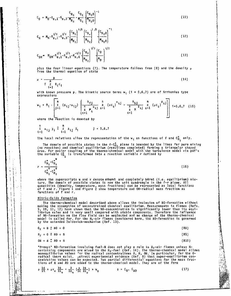
44

C 2 C0 CH 0 -

CO0 M O0*Ke 1 Ke 3 H 2. 0 2. 21 ~e,3H2 NO2 F 01

1/ 32 H 3/2 102 (12)

1/2 1/2

(' .- •i (13

5-1/2 3/2 -C2 0 H20

SH MOH" e,1e,4 e,3 12)1/2 2 2 'H ~

plus the four linear equations (7). The temperature follows from (8) and the density pfrom the thermal equation of state

P p(14)

T . Ric ii= I

with known pressure p. The kinetic source terms wi (i = 5,6,7) are of Arrhenius typeexpressions

wn=l f_ _ knW) I k f j n ,_ _, ,_ _, ,_ _ _wi = M "[ Biia"")i ' n nI (oct) n (pct)

l = M j1 H i=5,6,7 (15)

where the reaction is denoted by

n n01 Xij + Bij Xi J 5,6,7i~l i=1

The local relations allow the representation of the wi as functions of f and C2 only.2

The domain of possible states in the f-Ch plane is bounded by the lines for pure mixing(no reaction) and chemical equilibrium (reacions completed) forming a triangular shapedarea. For easier coupling of the thermo-chemical model with the turbulence model via pdf'sthe variable CA is transformed into a reaction variable r defined by

2

, CH2"CH 2

where the superscripts u and v denote unburnt and completely bOrnt (i.e. equilibrium) mix-

ture. The domain of possible states is now the unit quadrangle in the f-r plane. Allquantities (density, temperature, mass fractions) can be represented as local functions

of f and r. Figure 1 and figure 2 show temperature and OH-radical mass fraction asfunctions of f and r.

Nitric-Oxide formation

The thermo-chemical model described above allows the inclusion of NO-formation withoutmaking the assumption of unconstrained chemical equilibrium. Measurements in flames (Refs.9, 19, 11, 12) have shown that the NO-concentration is significantly lower than its equi-librium value and is very small compared with stable components. Therefore the influenceof NO-formation on the flow field can be neglected and no change of the thermo-chemicalmodel is called for. For the H2-air flames considered here, the NO-formation is governedby the extended Zeldovich-mechanism(Ref. 13).0 2 + N NO+ (RB)

N2 + 0 + NO + N (R) 4,OH + N NO + H (RIO)

"Prompt" NO-formation involving fuel-N does not play a role in H2 -air flames unless N- Acontaining components are mixed to the H2-fuel (Ref. 14). The thermo-chemical model allowsnonequilibrium values "nr the radical concentrations 0, H, OH; In particular, for the 0-radical there exist- ,,dire'ct experimental evidence (Ref. 8) that super-equilibrium con-centration values can be expected. Two partial differential equations for the mass frac-tions of N and NO are added to the thermo-chemical model. They are of the formP + CNI C (17)

at+ c ax - 7 u ax NOw

cc/

JA

JV/

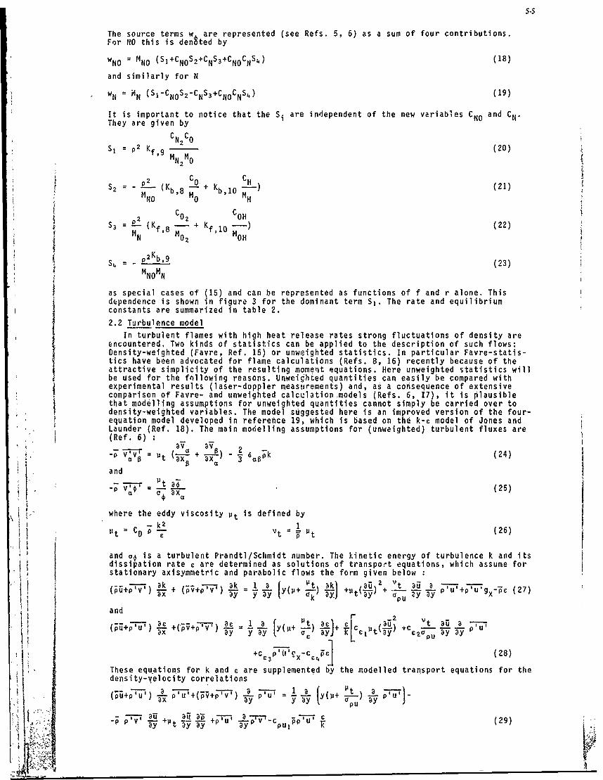
5-5

The source terms w are represented (see Refs. 5, 6) as a sum of four contributions.For NO this is denbted by

WNO = 14NO (S1+CNoS2+CNS3+CNoCNS ) (18)

and similarly for N

WN = 4N (SI-CNoS2-CNS +CNoCNS4) (19)

It is important to notice that the Si are independent of the new variables CMO and CN .They are given by

C CoCN2 0

, = p2 Kf, 9 (20)

MN2 0

CO- CHS- - b,8 Kb -) (21)

MNON '

S 2 02 OH3 - (Kf, 8 - + Kf,10 M ) (22)

N 02 OH

S4 =(23)MNO MN

as special cases of (15) and can be represented as functions of f and r alone. Thisdependence is shown in figure 3 for the dominant term S1 . The rate and equilibriumconstants are summarized in table 2.

2.2 Turbulence model

In turbulent flames with high heat release rates strong fluctuations of density areencountered. Two kinds of statistics can be applied to the description of such flows:Density-weighted (Favre, Ref. 15) or unweighted statistics. In particular Favre-statis-tics have been advocated for flame calculations (Refs. 8, 16) recently because of theattractive simplicity of the resulting moment equations. Here unweighted statistics willbe used for the following reasons. Unwei~hted quantities can easily be compared withexperimental results (laser-doppler measurements) and, as a consequence of extensivecomparison of Favre- and unweighted calculation-models (Refs. 6, 17), it is plausiblethat modelling assumptions for unweighted quantities cannot simply be carried over todensity-weighted variables. The model suggested here is an improved version of the four-equation model developed in reference 19, which is based on the k-c model of Jones and

Launder (Ref. 18). The main modelling assumptions for (unweighted) turbulent fluxes are(Ref. 6) I V ",a)" 7- Pt + ) - 6 k (24)

a aX a 3 as

and

-p = 0 ax (25)

I I where the eddy viscosity pt is defined by- k 2

Pt CDP Vt= P (26)P

and o€ is a turbulent Prandtl/Schmidt number. The kinetic energy of turbulence k and itsdissipation rate c are determined as solutions of transport equations, which assume forstationary axisymmetric and parabolic flows the form given below

( + 'V' + (Pv+P-) _2: :U a T YuP uk gx-6 (27)Ou-rr ak ay y ay a ) y .p

and puC -- ,) c =1 + P(+ 't 31 + c u t au a u

ax ay y ay (Y11 lit( ~ ou~

+C , c ; 0x c c (28)

These equations for k and c are supplemented by the modelled transport equations for thedensity-velocity correlations

a pu'+(FV+p'v) p-u , = 1a (y(,+ .t 2.. -T---u.-ax 7y aY a Pu ay

g" 2:0 +;7 2 p Pc p U (29)

By +tay ay ay u

anda( +P U PV'+(pV+pv) v T v - y+ ) '

-Ca + (30)

ay ay ay a PV 2(

In modelling the exact equations for k, c, 'u', p 'v', the expressions (24) and (25) andthe case of hiqh turbulent Re-numbers was assumed. From the latter follows in particularthat the correlation between quantities determined by different parts of their spectra isnegligible. Finally, the averaged mass and momentum equations are given by

(P+pu') + y(ZV+pv,) = 0 (31)

andaila 1u ap

(+( ;Vi.) 1 t(11+t) j +9 (32)

The constants for the turbulence model are given in table 1.

2.3 Probability density functions

Average values of the thermodynamic quantities can be calculated if the statisticalcharacteristics of the variables in the thermo-chemical model are known. It would besufficint to provide first and second order statistical moments of the variables f andr (or C"2 ) if the local relations would be close to linear. But the strongly non-linearcharacter of p(f,r), T(f,r), ci(f,r) requires the knowledge of the pdf (probability den-sity function) of f and r. Two different approaches to construct such pdf's will be dis-cussed.Method I

The pdf of the scalar variables f and r is constructed on the basis of a selected setof statistical moments. The general idea is to prescribe the functional dependence of thepdf on these moments. The crucial modelling assumption is obviously the explicit form ofthis dependence. Two different ways of establishing such forms will be considered.

F- In the first method the analogy between the pdf of fluctuating scalars in cold and non-reacting flows and the pdf of the reacting species in the'diffusion controlled limit(Ref. 20) is used to infer qualitatively the form of the pdf from measurements in incom-pressible flows. This was applied to the case of a single conserved scalar (Ref. 8) calledmixture fraction for the description of turbulent diffusion flames using the flame-sheetmodel. The measured pdf's (Refs. 21, 22) show strongly non-Gaussian features such assingular contributions reflecting the intermittent character of free shear flows and non-zero skewness. A reasonable fit with the experiments (Ref. 23) can be obtained if thefunctional dependence of single scalar pdf's on mean and variance is prescribed as beta-function.

P(x ,z) - ' (33)C, 1 1 -1aIdz z*l({1-z)

where the exponents are given in terms of mean f and variance g a (f-F)2 as

g (34)

and

The variable z denotes in (33) a possible value of the random variable f(xC,t). Thisfunction, however, is tot able to represent pdf's with relative maxima, which can be ex-pected in the outer 'prt of free shear layers (Refs. 21, 22). Other forms that have beensuggested are the clipped Gaussian and combinations of Dirac-pseudofunctions (Ref. 24).For the two dimersional pdf required here the following form of P(z,s) where s denotesa possible valne of the reaction variable r(xa,t), is put forward. First it is assumedthat mixture fraction f and reaction variable r are statistically independent. Hence

P(z,s) = P(z).P(s) (36)

Note that this does not imply- statistical irdependence of IF and CHV For P(z) the repre-sentation (33) as betafunction and for P(s) three Dirac-functions at r 0,1, are used AP(zs) za (1-z) 6-1 1(Y S (37)

5-7

The exponents a and B are determined by f and qaccording to (34) and (35). The nonnega-tive coefficients yl, Y2, Y3 depend on F and r as follows

y = rl (38)

r'

Y 2 =I (39)F(I-F)

Fr,2

Y3 = (40)I-?

At each p oi.t in the flow field the pdf P(z,s) is therefore determined by the four momentsf, g, IF, r'q for which modelled transport equations have to be solved (equations (45)-(48) below).

A second method was devised by Pope (Ref. 25) which relies solely on the informationprovided by statistical moments. The statistically most-likely distribution of a scalarf given the first L moments un is

L nP (z) = q(z) exp ( z Anz ) (41)L k=O

where q(.z) is the a priori probability of the samples of f(x,,t). It can be shown thatq(z) is constant for strictly conserved scalars and for scalars f obeying a transportequation with source term pS(f) it can be estimated for dominant S(f) by (Ref. 25)

q(z) = 1 + - S(z) (42)

where 'T is the time scale of dissipation of f. The coefficients An are determined bymaking the information entropy E

E f dz PL(Z) " - (43)

0

maximal under the side conditions

dz P(z) n O,(1),L (44)

0

of the available moments U3. This approach can be extended to any numnber of scalars. Cal-culations by Pope (Ref. 25) show that good agreement with experimental data for passivescalars can be achieved for L > 3. For the case of two scalars this would require at leastn.iZne moment equations.

Moment equationsThe four moment equations for the pdf in the form (37) can be obtained fromi (9) and

(10) together with (16) by applying the usual manipulations dnd averaging. The detailsof the closure operation are described in reference 26. For the f and g equations, themodelling follows closely the manipultions of the turbulence model described above. Theresulting equations are

) f + af 1 af( + t) 2 (45)ax. ay y ay iY3- Of 5yand

+ Y(~V) U 1 N A) 2 .i+ 2 +ax ay y y (y( 7c a ay) Of By+2t af a f. 't~ g (46)S+2 .2oJf r3 y a 9 ay ay

The derivation and modellitig of the equations for F and r'2 is more complex (Refs. 6, 26)and requires the consideration of the interaction between reactions and turbulent mixing.The result can be stated as follows:

I!(-i+p') ar + aP' l y1aI + -) - + (7a x ay ya ySc ar ay r~ 2 .I 47

j {: and

"--+ +(t+p-') a ! f -t -i2 A .. 2 -t -ax 57y yaP v A ay +2r aya-pr ay y

a -t (-Pr +22S

Vt W2 __ , +2r'-5 772(1-9-5F (48)ay ay k

where using (6) (see Ref. 26)W*H2

Sr w (49)

*v- *uand w M C C denotes the denominator of (16), and>, and w H2H2Mdeosa

x = 2w (50)w af 2

Noting that both quantities are functions of z and s we can evaluate their statisticalmomentsby integration using the pdf P(z,s).

For the calculation of the mean NO-mass fraction two additional partial differentialequations must be modelled. Averaging (17) for = NO and @ = CN and applying (25) leadsto

2 1 f,, _L ty'+ (51)ax gy y ay (A~+ a

where only the mean kinetic source terms NO and ;N require special c nsiderations. Firstwe note that the terms Si , i = 1, ...,4 in (18) and (19) can be represented as localfunctions of z ans s only, because they are a function of p, T, Co, CH, COH, CN, CO2which in turn are functions of f and r via the local relations. Hence we can eva uate themoments of wNO and wN'simply by integration using P(z,s). But the averaged source term

wNO = MNO S NO*S2CN S+NO'CN +C oS;+CN'Ss+CNO'CN'§4+C;o'S4'CN

* +CN'S4"CNO+CNO'CN'S4)

contains several correlations that cannot be calculated by integration. Remebering thatS, is the dominant source term :nd the fact that the mass fractions CNO and CN are smallcompared with the stable components, it is reasonable to neglect (for the NO-formation)these correlations. Then the equations (51) are closed with mean kinetic source termsgiven by

0 = MNO (S+C NO'S2+CN'S3+CNO'N'-4) (52)

and

W = MN (S1'CNO'Sa2CN'S3+CNO'CN 's ) (53)

The time scale ratio T appearing in (46) and (48) was estimated on the basis of recentmeasurements (Ref. 36) for a passive scalar in incompressible shear flows as

T - C 2n .12 + C:2 , = f,r

The values for C and C are given in table 1.Ti T2

This completes the coupling of the thermo-chemical model with the turbulence model usingthe method I for the construction of the pdf.

Method II

The second method avoids the explicit construction of the pdf P(z,s) in terms of sta-tistical moments by making use of the transport equation for P(z,s). Consider a set of niscalar variables *i(x ,t) satisfying transport equations of the form (17). The one-pointpdf P of the values zi of the *i(xat) can be defined by

mp( ilzi) a R S(Wixat)-zi)

nd

P(zi,x ,t) = <P>

where the angular brackets denote ensemble averaging. The transport equation for P followsaccording to Lundgren (Ref. 27) as

pp + Op-Pv P - <pv' > a (pS.P)+ ' (pr ) 1, P> (54)

t a BX a Bz z Xa ax az j ax a ax awhere the density and the sources Si are assumed to be local fuoctions of the *i (hence:=p(zi) and Sj = Sj(zi) in (54)) and the molecular L,-.aspbrt coefficients pri are con-stant and equal for a i = 1(1)m (Snvab-Zeldovich assumption). Equation (541 poses twomodelling problems (see Ref. 28) : the turbulent flux term and the scalar dissipationterm. On the other hand, the nonlinear sources Si pro-duce a closed term in the equation

I . M0

5-9

for the pdf P. This property is the main advantage of the transport equation (54). Forthe case of a single scalar variable (m=I) closure models (Refs. 28, 32, 33) have beensuggested. In particular, the turbulent flux term can be modelled by reference 32,

PVt aP-<Pv' p> 25 (55)Op x

This expression produces gradient-flux models for all higher correlations with the velocity.For the scalar dissipation term several stochastic models have been constructed. The inte-gral model suggested in reference 28

- <pr -L --L P> = P Tri dz' dz"P(z')P(z")(z',z",z)- (56)az ax ax k 11

P (z' ,z ,z) Z £therwise

has been applied to flame calculations on the basis of the flame-sheet model (Ref, 34)and gave satisfactory results. For two-scalar case considered here, the question of model-ling the cross-correlation

a2 af ar p-z-- <pr ax ax

is still not settled. Closure can easily be achieved using (55) and (56) if this term isneglected, but r is a transformed variable containing information about mixture fractionand therefore the usual argument of statistical independence at high turbulent Reynoldsnumbers does not apply. Further work on this problem is under way.,

3. APPLICATION TO H2-AIR DIFFUSION FLAMES

The closure modelldeveloped in the previous chapter was applied to several turbulentH2-air diffusion flames for which experimental results including NO-formation (Refs. 9,10, 11) are available. The discretization and numerical solution of the set of parabolicdifferential equations was performed with standard methods (Ref. 35).

Flame I (Refs. 11, 12).Kent and Bilger performed extensive measurements in several turbulent diffusion flames.

The horizontal flame simulated in our calculations is charecterized by the mean nozzle

exitvelcityU IO Tof H2 anddeosexit velocity Uj = 150 o 2 end 10, Re = 11700 (at nozzle exit) where Ue denotesthe velocity of the outer air stream. The initial conditions for the calculations aregiven by the measured profiles for mean velocity and turbulence energy. The initial dis-tribitions of mean mass fractions can easily be inferred from the nozzle conditions andthe dissipation rate is calculated from the condition of production equals dissipation inthe turbulence kinetic energy equation with prescribed turbulent viscosity. The resultsof the calculations are compared in figures 4 to 8 with the measurements. The agreementbetween the mean concentrations of the stable components and the mean temperature inexperiment and computation is very satisfactory. In the initial region for A < 80 the

Dcalculated profiles are spreading more rapidly than the experimental values (Figs. 4 and5), whereas the axial development is very well represented in figure 6. Several reasonscan be given for this overprediction of the spreading. The turbulent Schmidt/Prandtlnumbers are constant in the calculation, but values inferred from experiments show avariation from 0.4 to 1.0, furthermore are free shear flows highly intermittent and con-sequently the unconditional statistics of any flow quantity are highly non-Gaussian inthe outer part which cannot be described adequately by first and second order moments.The calculated profiles for the mean NO-concentration in figures 7 and 8 show that inaxial direction (Fig. 8) NO is underpredicted in the region A < 60, very well predictedin the medium range 60 < ! < 120 and overpredicted further downstream. In radial direc-

D xtion (Fig. 7), the profile for 80 is qualitatively correct but gives too small valuesin the core region due to the slightly larger spreading rate "F .he calculated jet.Flame 2 (Ref. 10)

Lavoie and Schlader performed measurements in a vertical H2-air diffusion flame withmean nozzle exit velocity of Uj = 200 m/s. The fuel H2 issues into still air and Re =4500 at the nozzle exit. The results of the calculations (Figs. 9 to 14) show the sameagreement between experiment and computation as flame 1 for stable components in figures9 and 10. The mean NO-concentration is again underpredicted for < 80 and very well

x Dpredicted for 1 > 80 as the axial development in figure 13 proves. The same figure con-tains in addition the results for a flame with Uj = 130 1 giving good agreement for

> 80 as well. The radial profilps in figures 11 and 12 reflect the axial underpredic-

tion at 40 and the good agreement for 80 and 120, 160.

|V

Flame 3 (Ref. 9)

The vertical flame measured by Takagi and Ogasawara has a mean exit velocity of U.108 r! and Re = 2200 and the fuel H2 issues into still air. The comparison of the concen-

trations of the stable components at = 50 shows the good agreement between experim, it

and calculation as flames 1 and 2. The NO-formation in this low Re number flame shows amuch slower decay of the mean NO-concentration along the axis than the previous flamesand the calculated values are smaller than the experimental concentrationd for x > 160

(Fig. 17). In the medium range the agreement is very good and the initial region is under-predicted as for flames I and 2. The calculated radial profiles in figure 15 are too small

Xin the core region for.6 < 80 but agree well in the outer part whereas for > 80 infigure 16 the core region is well represented.

4. CONCLUSIONS

A prediction model for turbulent H2 -air diffusion flames was developed that allows acertain degree of chemical non-equilibrium providing kinetic values for the 0, H, OH radi-cals that determine the NO-formation in such flames The results obtained with this modelwere compared with experiments in three different flames and lead to the following con-clusions

1. Stable components and temperature are well predicted. NO-formation is well predictedin the medium range of the flames, but underpredicted in the initial region and overpre-3 dicted (except for flame 3) far downstream.

2. NO-formation (calculated according to the extended Shvab-Zeldovich nechanism) is withinthe framework of this model very sensitive toward changes in the mean mixture fraction andthe mean reaction variable dnd in particular their variances. Those four quantities deter-mine the mean NO production rate via the pdf P(z,s). It could be expected that the formof the pdf has a strong influence on NO-formation. But figure 3 shows that NO-formationis restricted to a small part of the r-f 1ectanyle and hence does the form of the pdf notplay a ec isive role in the determination of mean NO-concentrations. This was supportedby numerical tests using different pdf forms (Ref. 6).

3. Comparison cf the two methods for constructing the pdf shows two distinct advantagesof the more elaborate transport equation approach. First is the modelling of moment equa-tions avoided, which could lead to inconsistent solutions because the closure assumptionsconsidered here do not guarantee the fulfillment of realizability conditions such as (refer-ences 5, 8)

g < f(1-f) etc

which are a consequence of boundedness of f and r. Second, the treatment of reaction kinet

tic source terms is straightforward and does not produce closure problems. On the otherhand, the transport equation (54) poses different closure problems and its numerical solu-tion requires for more than two scalars excessive computing times. Hence the second methodshould be considered a research tool to check and ease constructing pdf's as functionsof few momenrts.REFERENCES

1. WILLIAMS, F.A.: Combustion theory. Addison Wesley 1965.2. DIXON-LEWIS, G.; GOLDSWORTHY, F.A.; GREENBERG, J.B.: Flame structure and flame reaction

kinetics. Proc. Roy. Soc. London, A346, 1975, pp 261-278.3. DIXON-LEWIS, G. & RHODES, P.: Propertiesand kinetic mechanism in hydrogen-flames.

2nd European Combustion Symp., 1975, pp 473-478.4. STEPHENSON, P.L. & TAYLOR, R.G.: Luminar flame propagation in hydrogen, oxygen, nitrogen

mixtures. Comb. Flame, 20, 1973, pp 231-244.5. JANICKA, J. & KOLLMANN, W.: A two variables formalism for the treatment of chemical

reactions in turbulent H2 -air diffusion flames. 17th Symp. (Int.) Comb., 1978, toappear.

6. JANICKA, J.: Berechnung turbulenter Wassenstoff-Luft-Diffusionsflammen. Ph.D. Thesis,1979, RWTH, Aachen, Germany.

7. SPALDING, D.B.: Concentration fluctuations in a round turbulent free jet. Chem. Eng.Sci. 26, 1971, pp 95-107.

8. BILGER, R.W.: Turbulent jet diffusion flaies. Prog. Energy Comb. Sci., 1, 1976, pp 87-109.9. TAKAGI, T. & OGASAWARA, M.: A study of hitric oxide formation in turbulent diffusion

flames. 15th Symp. (Int.) Comb., 1975, pp 1051-1060.10. LAVOIE, G.A. & SCHLADER, A.F.: A scaling study of NO-formation in turbulent diffusion• flames of hydrogen in air. Comb.-Sci. Technol., 8, 1974, pp 215-234.

11. KENT, J.H. & BILGER, R.W.: Turbulent diffusion flames. 14th Symp. (Int.) Comb., 1973,pp 615-625.

12. BILGER, R.W. & KENT, R.E.: Further experiments on turbulent jet diffusion flames. 15thSymp. (Int.) Comb., 1974, op 541-551,

13. cOWMAN, C.T.: Kinetics of nitric oxide formulation in combustion processes. 14th Symp.(Int.) Comb., 1973, pp 729-738.

14. FENIMORE , C.P.: Effects of diluents and mixing on nitric oxide from fuel-nitrogen5. species in diffusion flames. 16th Symp. (Int.) Comb., 1976, pp 1065-1070.15. FAVRE, A.: Equations des gaz turbulents compressibles. Part II. J. de Mdcanique, 4,

1965, pp 391-421.16. JONES, W.P. & PRIDDIN, C.H.: Prediction of the flow field and local gas composition in

gas turbine combustion chambers. 17th Symp. (Int.) Comb., 1978, to appear.

I , . . .

17. JANICKA, J. ; KOLLMANN, W.; SAETRAN, L.; VANDROMME, D.: The modelling of turbulentfluxes in variable density flows. VKI, in preparation.

18. JONES, W.P. & LAUNDER, B.E.: The calculation of low Reynolds number phenomena with atwo-equation model of turbulence. Int. J. Heat & Mass Transfer, 16, 1973, pp 1119-1130.

19. KOLBE, W. & KOLLMANN, W.: Prediction of turbulent diffusion flames with a four equationturbulence model. Paper submitted to Acta Astronautica, 1979.

20. LIU, C-H & O'BRIEN, E.E.: Turbulent shear flow mixing and rapid chemical reactionsan analogy. J. Fluid Mechanics, 64, 1974, pp 195-206.

21. LaRUE, J. & LIBBY, P.A.: Temperature fluctuations in the plane turbulent wake.Ph:ysics of Fluids, 17, 1974, pp 1956-1967.

22. BATT, R.G.: Turbulent mixing of passive and chemically reacting species in a low speedshear layer. J. Fluid Mechanics, 82, 1977, pp 53-95.

23. RHODES, R.P.: A probability distribution function for turbulent flows, in TurbulentMixing in Nonreactive and Reactive Flows, Plenum Press, 1974, pp 235-241.

24. JONES, W.P.: Models for turbulent flow with variable density and combustion. VKI Lec-ture Series 1979-2.

25. POPE, S.B.: Probability distributions of scalars in turbulent shear flows. Proc. 2ndSymp. Turbulent Shear Flows, London 1979, pp 3.1-3.6.

26. JANICKA, J. & KOLLMANN, W.: Turbulence closure for flows with chemical reactions;in preparation, 1979.

27. LUNDGREN, T.S.: Distribution functions in the statistical theory of turbulence. Phys.Fluids, 10, 1967, pp 969-975.

28. JANICKA, J.; KOLBE, W.; KOLLMANN, W.: Closure of the transport equation for the pdfof turbulent scalar fields. J. Nonequil. Thermod., 4, 1979, pp 47-66.

29. HAY, J.H. & SICHEL, M.: Theoretical analysis of NO-formation near the primary reactionzone in methane combustion. Comb. Flame, 26, 1976, pp 1-15.

30. TSATSARONIS, G.: Vereinfachung des Methan/Sauerstoff Reaktionsmechanismus. Brenn.-W~rme-Kraft, 30, 1978, pp 249-255.

31. BAULCH, D.L.; DRYSDALE, D.D.; HORNE, D.G.: Evaluated kinetic data for high temperaturereactions. Butterworths, London, 1973.

32. POPE, S.B.: The probability approach to the modelling of turbulent reacting flows.Comb. Flame, 27, 1976, pp 299-312.

33. DOPAZO, C.: Relaxation of initial probability density functions in the turbulent con-vection of scalar fields. Physics of Fluids, 22, 1979, pp 20-30.

34. JANICKA, J.; KOLBE, W.; KOLLMANN, W.: The solution of a pdf-transport equation forturbulent diffusion flames. Proc. 1978 Heat Transfer Fluid Mech. Inst., Stanford U.Press, 1978i pp 296-312.

35. PATANKAR, S.V. & SPALDING, D.B.: Heat and mass transfer in boundary layers. Intertext,London, 1970.

36. WARHAFT, Z. & LUMLEY, J.L. : An experimental study of the decay of temperature fluc-tuations in grid generated turbulence. J. Fluid Mechanics, 88, 1978, pp. 659-684.

II

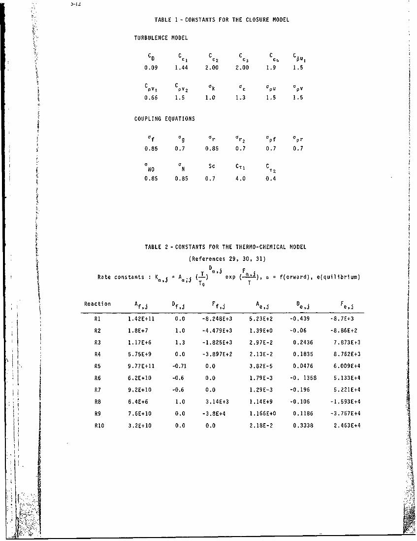
TABLE 1 - CONSTANTS FOR THE CLOSURE MODEL

TURBULENCE MODEL

CD C C C C CC 2 C3 C 4

0.09 1.44 2.00 2.00 1.9 1.5

C C 0r a

0.66 1.5 1.0 1.3 1.5 1.5

COUPLING EQUATIONS

a f a ar r apf apr

0.85 0.7 0.85 0.7 0.7 0.7

a a Sc Cr I CNO N '

0.85 0.85 0.7 4.0 0.4

TABLE 2 - CONSTANTS FOR THE THERNO-CHEMICAL MODEL

(References 29, 30, 31)

T Da FRate constants : , A";j (-) exp (.A,~ f(orward), e(quilibrium)

To T

Reaction A, Df, Ff Ae ~ De Fe.

Ri 1.42E+11 0.0 -8.248E+3 5.23E+2 -0.439 -8.7E+3

R2 1.8E+7 1.0 -4.479Ei*3 1.39E+O -0.06 -8.86E+2

R3 1.17E+6 1.3 -1.825E+3 2 .97E-2 0.2436 7.873E03

R4 5.75E+9 0.0 -3 .897E+2 2.13E-2 0.1835 8 .762E+3

R5 9.77E+11 -0.71 0.0 3.82E-5 0.0476 6.009E+4

R6 6.2E+10 -0.6 0.0 1.79E-3 -0. 1358 5 .133E+4

R7 9.2E+10 -0.6 0.0 1,29E-3 -0.196 5.221E+4

R86.4E+6 1.0 3.14E+3 1.14E+9 -0.106 -1.593E+4

R9 7.6E+10 0.0 -3.8E+4 1.166E+0 0.1186 -3.767E+4

R1O 3.2E+10 0.0 0.0 2.18E-2 0.3338 2.463E+4

- - - 0C 14400

20 207 7i120\C600 400

0 10~ 03 000 0 0 0

t~ll 0 220

Fig. 1. Temperature as function of Fig. 2. Molar concentration of OH asmixture fraction f and reaction function of f and r.variable r.

- 100

000 0.I3O

00 0

02000 - 0

0 1 3 0$ 00 2 0 0 90 10

0<H 2 0

900

40

fil 1 0.

-ig 3. -oinn sorc ter of FIg. 4. Rda itibto fmaNO teprtr anducio mea fuolaro concen-r

traton at 2 / 0frf~e1

0.y, 0

or tin at xD 80 fo flam 1.ii0

ff~o N

Fig Re f ea12

0O 040

000 02-----------------------------

0I 0 A 0 -1

0 20 40 60 80 0 120 14 0 160 1 0 -200

Fig. 6. Axial distribution of meantemperature and mean molarconcentration for flame 1.

020,

NO 0

4600

024 A

00

00

a 0 0 80 O 0

, o OC /

0' 0 8 12 16 20 28 3 0 20 /a36D

Fig. 7. Radial distribution of meanNO - mass fraction at x/D 080 for N mass fraction for flame 1.t flame 1.

028

024,-II

/ "02

2 "2

0 0 O 8 2 16 20 2 4, 28 3 2 y/0 36

S ,Fig. 9. Radial distribution of

mean mass fractions at x/D ='40~for flame 2.

f

5-L5

02& ~ - -

o I ...... ........ ......L......02:2

- - -- Ret. 20

0 0 0 0a 0 2 C M2

00 11 __

0 8 15 24 36 x 0

Fig. 10. Radial distribution ofmean mass fractions at x/D = 160for flame 2.

0" . 0 0 0 .,O.'O . . 10

6C260

0-SNS.4

0 a 1, 2/ 32 0/0 36 0 a 16 24 32 40 Y/o

Fig. 11. Radial distribution of mean Fig. 12. Radial distribution of meanNO - mass fraction at x/D ='40, NO - mass fraction at x/D = 120, 16080 for flame 2. for flame 2.

ENO EopewMCN----------------, -

120-

0 0 80 ;20 160 x 200

Fig. 13. Axial distribution of mean

NO - fraction for flame 2.

- - -Fig. 14. Radial distribution of meanSepiments molar concentrations at x/D 25, 50Re.9 for flame 3.

0 02 ' 6 H2

0 232--

- -

0 *-/O'5024 20 200 ,

6 160H2020

16_

00 0

0- 0

0 t0 20 30 40 oY/b

\ Fig. 15. Radial distribution of mean0 ,NO -concentration at x/D =25 50

0 20 30 for flame 3.

20

- -- Ee .ments

PPM040 x/D-1500 0

260 0 X/0-- ---- 0

0

0 t0 20 30 4.0 50

Fig. 16. Radial distribution ofmean NO - concentration at x/D = 100,150 for flame 3.

-2It J

200 ---- - - -

160--- -- -

'> 1 01 0-S ,i o

2o00Io e o o

0 4.0 80 120 160 200

Fig. 17. Axial distributiont of meanNO - concentration for flame 3.

fy

5-17

DISCUSSION

N.Peters, GeIn a recent study [ 1 ] of the first author with myself we could show that the local NO-formation does depend onthe scalar variance, the total NO-formation does not.

By evaluating the mean turbulent NO reaction rates in the limit of large NO-activation-energies we could decouplethe influence of turbulence from that of the kinetics. We found that higher variances of the mixture fractions wouldspread the NO-production over a larger volume and into the fuel rich part of the flame but that its integral over theflame volume would ot change considerably.

[1 ] J.Janicha Evaluation of the Turbulent NO-Production Rate in the Limit of Large ActivationN.Peters Energies, submitted to Combustion, Science and Technology.

Author's ReplyThat superstates my own conclusion.

F.C.Lockwood, UK(1) It seems to me that the overall reaction in the flames you have examined must be largely turbulence rate

controlled. In this respect how would your calculations compare with those assuming an infinitely fast reactionrate?

(2) Can you offer any physical arguments in support of your three Dirac function assumption for P(s)? The oneat F would seem least satisfactory.

Author's Reply(1) Infinitely fast reactions can easily be simulated in our program by setting the reaction variable to unity. There

is little influence on mean density, temperature and concentrations of stable components. The mean radicaland NO concentrations show marked difference to the complete modei.

(2) A physically more satisfactory form of the pdf could be obtained b" solving tlht pdf-transport equation aspointed out in the paper. For the current calculations the form of rks) was chosen that seemed appropriatewith respect to the dependence of the NO-source term S, on f and r.

A.K.Varma, USOnce a model for the pdf has been established, it is of course possible to calculate all the turbulence/chemistry inter-action correlations in the equations for r, f, r etc. Did you include all these terms - specially third-order correla-tions - in the source terms in the transport equations?

Author's ReplyAll correlations of functions of mixture fractions f and reaction variable r were of course evaluated by integrationusing the pdf.

C.H.Priddin, UKThe applicability of your joint PDF depends strongly on the assumption of Equation (36) that the PDF is separableinto two parts (covariance of Z and S zero). Do you have any information to indicate how good this assumption is?

Author's ReplySince there is no experimental information for the simultaneous pdf P(f, r) available the computationally mostefficient fon was adopted. Numerical tests using different forms of the one-dimensional pdf's constituting P(f, r)

* showed little influence on the mean NO-profiles (see Reference 6). More general pdf's P(f, r) are currently-investigated.

6-I

TURBULENT REACTION AND TRANSPORT PHENOMENA IN JET FLAMES

BY

H. EICKHOFF, Institut fUr Antriebstechnik, DFVLR, Linder H6he, 5000 K6ln 90, W.Germany

K. GRETHE, Lehrstuhl fUr Feuerungstechnik, Universitat Karlsruhe,Richard-Willstitter-Allee, 7500 Karlsruhe, W.Germany

F. THIELE, Hermann-Fbttinger-Institut, Technische Universitdt Berlin,Strafe des 17. Juni 135, 1000 Berlin 12

SUMMARY

A new reaction model accounting for intermediate species was applied in connectionwith the k-c-model to predict different free and enclosed turbulent natural gas flames.The reaction model is based on the assumption of a quasilaminar flame substructure of aturbulent diffusion flame and a probability density distribution of fuel-atom-concentra-tion. It is assumed, that the quasilaminar flames are in local chemical equilibriumwithin zones of finite thickness.

The influence of variable density on the mixing prozess was studied for differentjets and jet flames. In the parabolic flow cases it was found necessary to account forvariable density which was done by a mixing length relation. Different numerical pro-cedures w ere applied for the parabolic and elliptic flow fields

LIST OF SYMBOLS

c mass fraction

cA mass fraction of fuel atoms

d nozzle-diameter

f transformed stream function

k kinetic energy of turbulence

1 mixing lengthP probability density function

Q general variable, Eq.(3.5)

S source term

T temperature

u,v velocity components

x,r coordinates

z similarity parameter

a intermittancy

e dissipation

E ,r transformed coordinatesstream function

|P density

turbulont shear stress

effectivw viscosity4) general variable, Eq.(3.1)

r general transport coefficient

Subscripts

w outer boundary

c centerlineI

1. INTRODUCTION

The main problem in modelling turbulent combustion for engineering applications is todevelope appropriate simplifications for the complex phenomena of chemical reactions andturbulent transport.As a simple and useful way to account fo: the influence of turbulence on chemical re-actions, the flame sheet assumption was introduced and coupled with a probability densitydistribution of the concentration of fuel atoms.As in fuel rich regions of hydrocarbon flames especially the existence of carbon monoxidcannot be neglected the flame sheet model was extended [1].

2. THE REACTION MODEL

The instantaneous gas composition in the flame sheet approximation, with reactionstaking place only in an infinitely thin layer, is a mixture of stoichiometric reactionproducts and either fuel or oxident in the fuel rich and fuel-lean regions, respectively.In the present model it is assumed that the turbulent diffusion flame exists of a brushof quasilaminar flames in local chemical equilibrium within zones of finite thicknessand a frozen flow outside.

In Fig.1 as an example the instantaneous CO-concentration and temperature are shownas function of the mass fraction of fuel atoms cA. To define the boundaries of the equi-librium zone it would be necessary to know the characteristic flow and chemical times.

For reasons of simplicity we introduce a critical temperature at cA1 in the fuel rich

region below which the reactions freeze, as it was first done by Libby [2] for a laminarboundary layer combustion.

Since the concentrations of intermediate species are close to zero at the reactionzone boundary on the fuel lean side, equilibrium can be assumed throughout the fuel leanregion. If the flame approximately can be assumed to be adiabatic with respect to itssurrounding then it is not necessary to solve an energy balance equation to calculatethe temperature and gas composition, which are obtained from an adiabatic equilibriumcalculation if the fuel mass fraction c is known.

cA4Otherwise a non adiabatic equilibrium calculation has to be performed and in addition

the energy equation has to be solved.

To calculate the equilibrium-zone composition and temperature, a computer program ofPratt and Wormeck (3) was used. In the fuel rich region I, ., our crude assumption isthat the gas is a mixture of unreacted fuel and an averaged concentration of products ofthe equilibrium zone.

The steps of the temperature and concentrations at the freezing boundary CA1 of

cause are physically unrealistic because of finite reaction rates and molecular diffusion.But as v'e are dealing with a highly turbulent flow this simplifying assumption may beadapted.

To account for the influence of turbulent fluctuations we introduce a probability

density function for the mass fraction of fuel atoms P(cA). It is a modified Gaussian

function and was derived by Haberda [4), based on experiments.

Mean values of the flow variables are obtained, if the instantaneous values 4 (cA)of the flame zone approximation, Fig.1, are introduced from the relation [4]:

4 CA) a (cA) P(cA) dcA + (1 - a) P (2.1)

0

with a as the intermittancy factor being a function of the turbulence intensity of theconcentration fluctue ions.

,I

6-i

3. BASIC EQUATIONS

The conservation equations for two-dimensicnal flows can be written in the generalform

ax r Dr x 0 ax r ar (r ar 4 (13.1)

* with

4 = u,vcA,k,c,c2A'

The set of equations given by Eq.(3.1), the equation of state and Eq.(2.1) includingthe flame zone approximation, Fig.1, determine the problem.

3.1 Jet Flames of Boundary Layer Type

For jet flames of boundary layer type Eq. (3.1) in terms of the x-momentum equationbecomes after an order of magnitude analysis for large density fluctuations

( - 1), as derived by Bray [5]

D(u2) 1 a(r p u) + a ( _ + -, +p S3ax r ar a v' u v =5 u (3.2)

with S for the buoyancy term.

Introducing a stream function ' by

= _ (T)r, - _U r (3.3)ax 3r

and neglecting the term V Tru' of the turbulent shear stress in Eq. (3.2) only the triple

correlation pTu'vl remains which has to be modelled for variable density flows ofboundary layer type in addition to incompressible flows.

Here we introduce the simple assumption

- p'u'v' = cO u T ar (3.4)

where c is an empirical constant which has to be determined from experiments and 1 is

a mixing length.

The term 717 is given by the known k-c-model

u, ----rk 2 au

D,r ar3

where cDr is an empirical expression.

With Eqs.(3.4) and (3.5) the turbulent shear stress becomes

akc ar

Tt li (p ar cD,r k ar (3.6)

, f4. NUMERICAL PROCEDURE

For free burning jet flames of boundary layer type a numerical procedure is appliedwhich has been derived by Thiele [6]. The numerical procedure for predicting he e.llipticfl(w field was taken from [7].

Before the parabolic differential equations according to Eq. (3.2) are solved numeri-cally, the following similarity transformation [8] is applied

x r

(pP )C dx, = prdr/ 2K (4.1)

with the transformed stream function

(4.2)

The value of K is equal to zero in the initial jet region uc u and 4 furtherdownstream. With this transformation the x-momentum becomes

zfq + {z + Kf + if) f + (Kfq - Kf. )fn Su (4.3)

with n

z 2 pp t/(P1t)c • dri/p (4.4)

If the value of z is a function of n only (for constant density and eddy viscosityz = 2 n) then a similarity solution is obtained from Eq.(4.3) and accordingly from theother balance equations. Although there are deviauions from similarity in turbulent jetflames, the "similarity"-transformation is useful if the equations are to be solved nu-merically as the flow variables vary slowly in the main flow direction.

The transformed differential equations can be written in the general form

a Q Mn + b Qnn + c Qn + < Q + e Q., = g (4.5)

where Q represents the stream function, element mass fraction etc.By applying the wellknown backward finite-differences in g-direction the parabolic differential equation isreduced to an ordinary differential equation. This equation is solved by the finite-diffe-rence method of Hermitian type. The high accuracy of the method results from the fact thatthe grid point values of the function and the first derivative are used for the approxi-mation of the higher derivatives. Thus we get a considerable reduction in the number ofgrid points used. Furthermore, for the momentum equation which is of third order and theelement mass fraction equation which is of second order the finite-difference approxi-mation yields a 2 x 2 block-tridiagonal system of finite difference equations which canbe solved by a Gaussian elimination procedure. Due to the transformation only few itera-tions are necessary to solve the nonlinear momentum equation. An additional advantageof the transformation is that boundary conditions u(n,)> 0 can be satisfied withoutdifficulties.

2The system of conservation equation (4.5) of the unknowns f, c , cl , k and c has

been solved with the constants of the closure assumptions as given n Tble 1 and theadditional empirical relations discussed below.

Table 1 (Symbols as defined in [7]).

c c c a c c a a1 2 D k C g I g2 c g

1,43 1,92 0,09 1,0 1,3 2,8 2,0 0,7 0,9

The influence of the value of the empirical constant c in Eq.(3.6) was studied nu-mericallv and was found to be approximately 1.5. P

As known from Rodi's investigations (91 on free turbulent shear flows there exists

no universal set of constants. To get agreement of prediction with experiment for roundjets the value of c0 was modified (9]. Other proposals have been made also [10].

To account for the curvature effect in a round jet we prefer for simplicity andphysical plausibility the following modification of cD for round jets

r+cr ccD,r cD r+l (4.6)

where cr is an additional empirical constant, which was found to be 0.78.

The mixing length 1 in Eqs.(3.6) and (4.6) is given by k and e through the relation

1 k 3/2/C.

5. RESULTS

The influence of the additional constants c and cr accounting for variable density

and curvature effects were investigated systematically for parabolic flows.First investigations concerned different non reacting jets with density differences

due to the mixing of two different gases (H,-air and C0O.-air).

Results are shown in Fig.2, where predictions are compared to experimental values [11, 12].

The larger spreading rate of the hydrogen jet in terms of (PU2)/(Pu 2 ) ratherwell predicted with the constants cr= 0.78 and c. = 1.5. 0 is

I~r

NV)

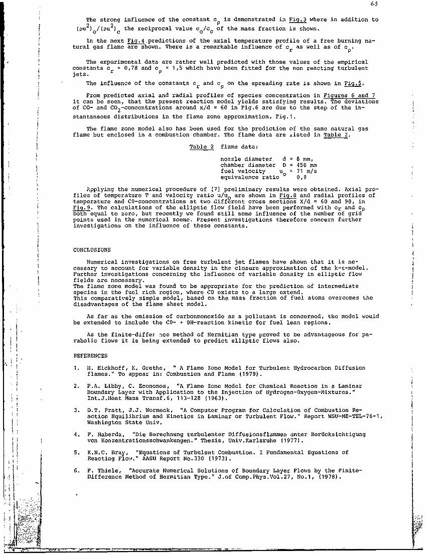
6-5

The strong influence of the constant c is demonstrated in Fig.3 where in addition toP2 th2eirclvlec/(pU2)o/(pu2)c the reciprocal value cI/uc of the mass fraction is shown.

In the next Fig.4-predictions of the axial temperature profile of a free burning na-tural gas flame are shown. There is a remarkable influence of cr as well as of c

The experimental data are rather well predicted with those values of the empiricalconstants c = 0,78 and c = 1,5 which have been fitted for the non reacting turbulentjets. r p

The influence of the constants c and c on the spreading rate is shown in Fig.5.r p

From predicted axial and radial profiles of species concentration in Figures 6 and 7it can be seen, that the present reaction model yields satisfying results. The deviationsof CO- and C02-concentrations around x/d = 60 in Fig.6 are due to the step of the in-

stantaneous distributions in the flame zone approximation, Fig.1.

The flame zone model also has been used for the prediction of the same natural gas

flame but enclosed in a combustion chamber. The flame data are Listed in Table 2.

Table 2 flame data:

nozzle diameter d = 8 mm,chamber diameter D = 450 mmfuel velocity uo = 71 m/s

J equivalence ratio 0,9

Applying the numerical procedure of 17] preliminary results were obtained. Axial pro-files of temperature T and velocity ratio u/uo are shown in Fig.8 and radial profiles oftemperature and CO-concentrations at two different cross sections X/d = 60 and 90, inFig.9. The calculations of the elliptic flow field have been performed with cr and cpboth equal to zero, but recently we found still some influence of the number of gridpoints used in the numerical sceme. Present investigations therefore concern furtherinvestigations on the influence of these constants.

CONCLUSIONS

Numerical investigations on free turbulent jet flames have shown that it is ne-cessary to account for variable density in the closure approximation of the k-s-model.Further investigations concerning the influence of variable density in elliptic flowfields are necessary.The flame zone model was found to be appropriate for the prediction of intermediatespecies in the fuel rich region, where CO exists to a large extend.This comparatively simple model, based on the mass fraction of fuel atoms overcomes thedisadvantages of the flame sheet model.

As far as the emission of carbonmonoxide as a pollutant is concerned, the model wouldbe extended to include the CO- + OH-reaction kinetic for fuel lean regions.

As the finite-differ nce method of Hermitian type proved to be advantageous for pa-rabolic flows it is being extended to predict elliptic flows also.

REFERENCES

1. H. Eickhoff, K. Grethe, " A Flame Zone Model for Turbulent Hydrocarbon Diffusionflames." To appear in: Combustion and Flame (1979).

2. P.A. Libby, C. Economos, "A Flame Zone Model for Chemical Reaction in a LaminarBoundary Layer with Application to the Injection of Hydrogen-Oxygen-Mixtures."Int.J.Heat Mass Transf.6, 113-128 (1963).

3. D.T. Pratt, J.J. Wormeck, "A Computer Program for Calculation of Combustion Re-action Equilibrium and Kinetics in Laminar or Turbulent Flow." Report WSU-ME-TEL-76-1,Washington State Univ.

4. F. Haberda, "Die Berechnung turbulenter Diffusionsflammen anter Berucksichtigungvon Konzentrationsschwankungen." Thesis, Univ.Karlsruhe (1977).

5. K.N.C. Bray, "Equations of Turbulent Combustion. I Fundamental Equations ofi ! Reacting Flow." AASU Report No.330 (1973).

6. F. Thiele, "Accurate Numerical Solutions of Boundary Layer Flows by the Finite-Difference Method of Hermitian Type." J.of Comp.Phys.Vol.27, No.1, (1978).

U

7. W.M. Pun, D.B. Spalding, "A General Computer Program for Two-Dimensional EllipticFlows,". Report HTS/76/2, Imperial College of Science and Techn., Mech.Eng.Dep.London.

8. F. Thiele, "Die nunerische Berechnung turbulenter rotationssymnetrischer Frei-strahlen und Freistrahl-Diffusionsflanmen." Thesis, Univ.Karlsruhe (1975).

9. W. Rodi, "The Prediction of Free Turbulent Boundary Layers by Use of a Two-EquationModel of Turbulence." Thesis, Umiv.of London (1972).

10. S.B. Pope, "An Explanation of the Turbulent Round-Jet/Plane - Jet Anomaly.AIAA-Journal, Vol.16, No.3 (1978).

11. B. Lenze, R. Gunther, "Ausbrand und W~irmeentwicklung in Erdgas-Diffusionsflammen."1Brennstoff-Wdrme-Kraft, 17: 387-394 (1975)

12. Engler-Bunte-Institut der Universit~t Karlsruhe (T.H.), Bereich Feuerungstechnik,Prof.R.Gunther (private communication).

10

2000Vol%!

T Co1000 5

C o

K 0

CA

Fig. 1: Instantaneous temperature and CO-concentration as function of massAfraction of fuel atoms CA 1

V-

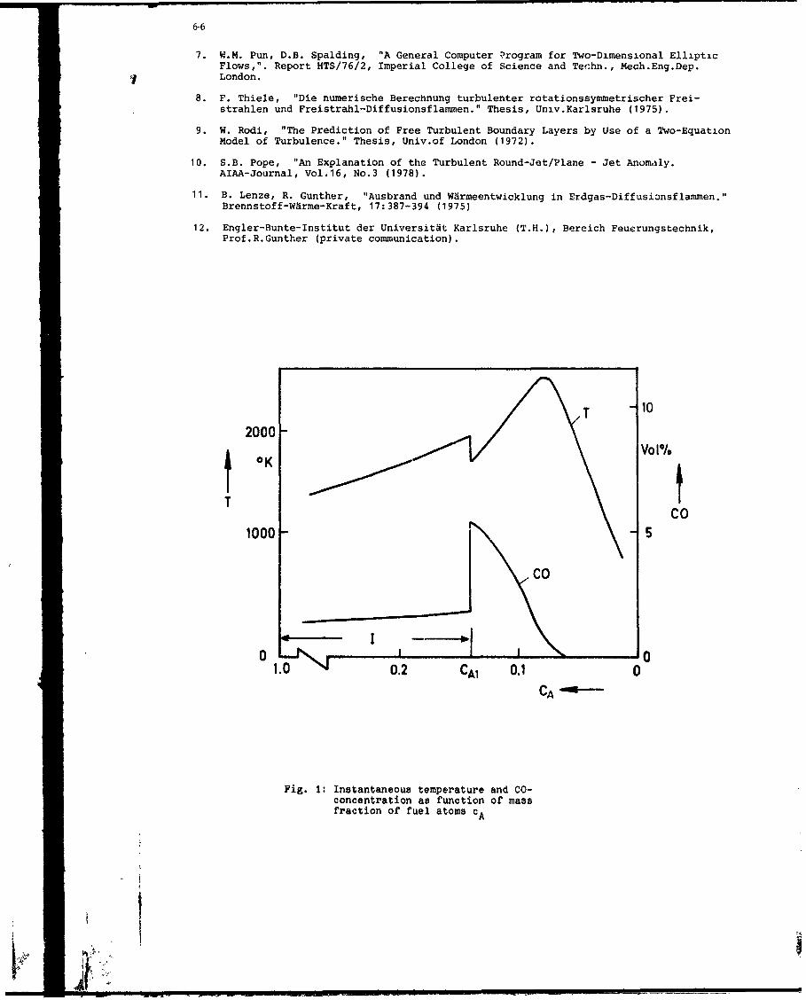
6-6

7. W.M. Pun, D.B. Spalding, "A General Computer ?rogram for Two-Dimensional EllipticFlows,". Report HTS17612, Imperial College of Science and Techn., Mech.Eng.Dep.London.

8. F. Thiele, "Die nuxnerische Berechnung turbulenter rotationssynmetrischer Frei-strahlen und Freistrahl-Diffusionsflammen." Thesis, Univ.Karlsruhe (1975).

9. W. Rodi, "The Prediction of Free Turbulent Boundary Layers by Use of a Two-EquationModel of Turbulence." Thesis, Univ.of London (1972).

10. S.B. Pope, "An Explanation of the Turbulent Round-Jet/Plane - Jet Anomaly.AIAA-Journal, Vol.16, No.3 (1978).

11. B. Lenze, R. Gunther, "Ausbrand und Warmeentwicklung in Erdgas-Diffusionsflammen.'Brennstoff-Warme-Kraft, 17: 387-394 (1975)

12. Engler-Bunte-Institut der Universitdt Karlsruhe (T.H.), Bereich Feuerungstechnik,Prof.R.Gunther (private communication).

2000-

Vol%.

T Co

1000 - C

C o

0 0

10 02 CA 0.1CA 0

Fig. 1: Instantaneous temperature and CO-concentration as function of massfraction of fuel atoms CA

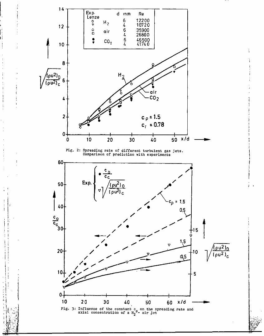
Exp. d mm ReLenze

o H2 6 1220012 4 10720

air 6 35900o 4 26800

10 _ C02 4 417_,_4500

8

l pU2 )0 H

420- air

4-- -C02

2- cp 1.50 Cr =0.78

0 ~ I I i I I0 10 20 30 40 50 x/d - .

Fig. 2: Spreading rate of different turbulent gas jets.

Comparison of prediction with experiments

60,

Cc

50- Exp. F(pu2 0

//

40 Cp1.540 0.5

C0 /

C

3 0 -- 0000 .00, I1 5

20- / -10)

'-,1 0 30 40 50 60 x/d - -I t /0"0

A ,0 40Fig. 3: Influence of' the constant c on the spreading rate and

axial concentration of a H2air jet

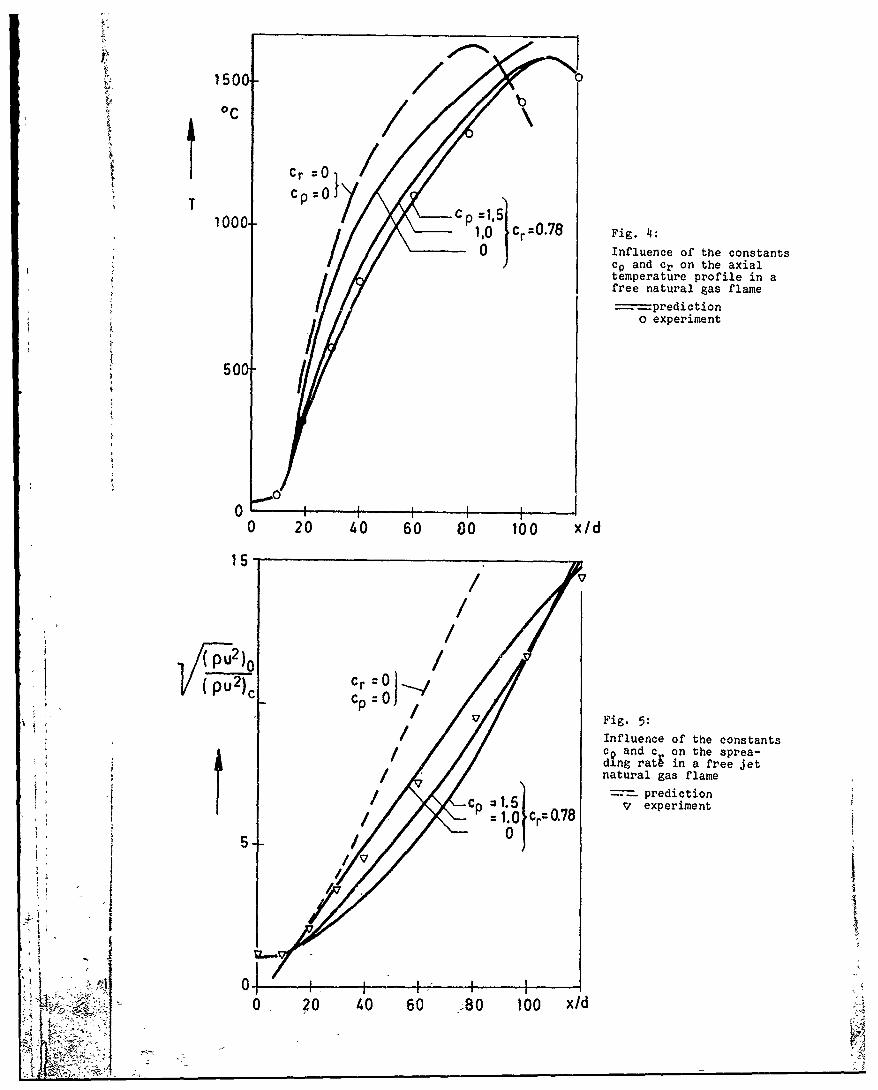
150G

0C

T 100 0 1 P = ,

cp and cr On the axialtemperature profile in afree natural gas flame

-.predictiono experiment

0 20 40 60 80 100 xld

(pu 2)c /r=

/v Fig. 5:/ Influence of the constants

cq and c on the sprea-ding rat9 in a free jet

1' / Vnatural gas flame

1 / Cp ~1.0 } Crza078/0

0S0 20 40 60 -80 100 xld

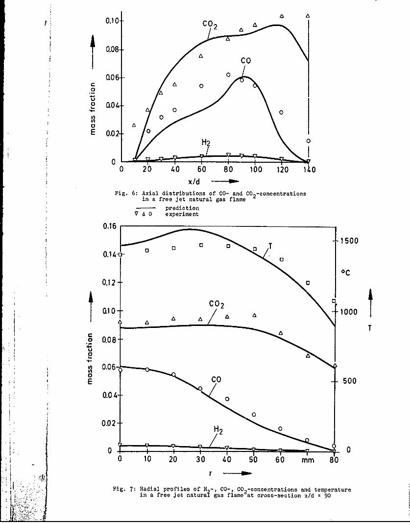
0.10

T0.08-CC

00

O 0.04

4- 4

(n

0

00

0 20 40 60 80 100 120 110xld so"

Fig. 6: Axial distributions of C0- and C02-concentrationsin a free jet natural gas flame

prediction7 A 0 experiment

0.16

_1500

OC

0.1 2-

Kt 0.10 C0 t000V T

C&o0.08-

00

0.06

0.0 0

I in a 0 fre jet0 6 mm 80

Fig. 7:Radial prof~iles of H -, C0-,C cnetain n temperaturein fee etnaturai gas flame at cross-section x/d 90

to tO T 0 01500

0 0

13500

0 T0.5

1500

Fig. 8: Axial temperature T and velocity u/u0 ianecodntulgas f'lame 0i necoe aua

-predictiono) 0 experiment

1500'7 0

OC

V0

0

0

T 0T Co

0 o o Volq/%0

60 65 0006

460 90

00 8 16 20 24

ri/d Do-Fig. 9: Radial profiles of temperature T and CO-concentration in

an enclosed natural gas flameprediction7V00 experiment4

DISCUSSION

J.H.Whitelaw, UKIt is likely that the round-jet anomaly does not occur in the sense that the k-e model can calculate the plane jetand not the round jet. It is more likely that the k- e cannot predict the spreading rate of either, if "flapping" and"room draughts" are present. Bradshaw has shown that the spreading rate of the flame jet, with its far-down streammeasurements, is increased by the low frequency effects of flapping and draughts and that, without thesephenomena, the spreading rate would be the same as for the round jet. Our own measurements show that flappingdoes not occur in round jets.

Author's ReplyWe agree that the k-e model cannot predict the spreading rate ofjets if flapping is not taken into account. But inour opinion the gradient diffusion approximation for a transported quantity t1 in its' usual form:

Vt a(I)ao 3ir

should be modified in order to account for the influence of curvature, see also Spalding (*)

( ) Spalding, D.B. Turbulent Mixing in Nonreactive and Reactive Flows, ed. by S.N.B.Murthy, p. 102,(1975).

AK.Varma, USEarlier in Paper 5 we saw good results obtained for Hydrogen-Air flames by the use of a turbulence model that usedthe basic k-e model unchanged but added equations for p'u' and p'v'. Can you reconcile your modifications ofthe k-e model for the effects of density variation with the results of Kollman?

Author's ReplyKollman and our approach are dif ferent but it cannot be excluded that they yield similar results. We demonstratedin our presentation the effect of ou_modification of the k-e model and it would be interesting to see the effectof using additional equations for p'u' and p'v as Kollman did it.

From our own investigations we know that the influence of variable density in turbulent hydrogen flames is less thanin hydrocarbon flames.

N.Peters, GeI would like to point out the difference between the flame zone model of Libby and Economos and your model.In the flame zone model freezing at a certain temperature results in a jump of the slope of the temperature andconcentration profiles while your model assumes the jump of the value itself. The flame zone model was shown tocorrespond to the large activation energy limit for a one-step reversible reaction'. I doubt that a jump conditionfor the values of the dependent variables can be justified in a rational way.

1. Peters, N. Premixed Burning in Diffusion Flames - the Flame Zone Model of Libby andEconomos. Int. J. of Heat and Mass Transfer, Vol.22, pp. 69 1-703, (1979).

Author's Reply,In principle you agree with our statement in Chatper 2.

Th.T.A.Paaw, Ne

Did you measure oxygen concentrations on the centre-line of your natural gas flame, and if so, have you comparedthis with your predictions?

Author's Reply

Yes we compared our predictions to the measurments of 02 in the natural gas flame. We obtained in generalsatisfying agreerment except at the beginning of the flame where we had an underprediction of oxygen. This is dueto the fact, that there have been problems with flame stabilisation. This has not been taken into account in ourprediction.

11:3 '

I-!I

ON THE PREDICTION OF TEMPERATURE PROFILES

AT THE EXIT OF ANNULAR COMBUSTORS

Osama M.F. Elbahar and Sigmar L.K. WittigInstitut fUr Thermische Str~mungsmaschinenUniversitat Karlsruhe (TH), Kaiserstr. 12

D-7500 Karlsruhe 1

SUMMARY

Despite their inherent limitations, two-dimensional predictionprocedures based on solving the basic equations and incorporating thek-c model of turbulence are shown to be effective tools in designingannular combustors. In comparing the results it is found that predic-tions from available jet mixing correlation data within certain limi-tations will represent measurements from single row injection moreaccurately. Detailed calculations, however, will be more effective inpredicting opposite wall cooling air injection, multiple row jetmixing, heat transfer, film cooling and the effects of convergingcombustor exit. Because of its relative simplicity, the predictionprocedure is particularly suited for design parameter studies.

LIST OF SYMBOLS

B slot width

Cd hole discharge coefficient

C a constant in the turbulence model

D hole diameter

H duct or combustor height

h enthalpy of fluid

J momentum flux ratio

, k Kinetic energy of turbulence

mass flow rate

S spacing between the centerlines of two adjacent holes

S source term in the conservation equation of the variable

T absolute temperature

u x-component of velocity

v y-component of velocity

W width

x distance in flow directio,-

y distance in direction perpendicular to xz distance in direction perpendicular to both x and y

r exchange coefficient for the variable *1i fluid viscosity

p density

0 dimensionless temperature ratio

C dissipation of turbulence energy

V general notation of a dependent variable

Subscripts

C jet centerline

eff effective

j related-to the cooling air jet

min minimum

t turbulent

w wall

*€ related to the variable *1/2 half quantity

-related to mainstream

Superscripts

+ plus side, or side away from jet entrance wall

- minus side, or side toward jet entrance wall

1. INTRODUCTION

Recent attempts to increase the specific power or thrust and to reduce the specificfuel consumption of jet engines as well as of stationary gas turbines necessitates ope-ration under high turbine inlet temperatures. Elevated inlet temperatures imply increa-singly stringent limitations upon the temperature profile at the entrance to the turbine,i.e. exit of the combustor. Hot gas temperature profiles must be matched carefully toturbine blade stress levels if long turbine life is to be attained. For this reason, pre-diction techniques for the temperature profile at the combustor exit have become of pri-mary importance,

The develrpment of the temperature profiles depends primarily on the mixing processbetween the cooling air and the hot gas flow in the mixing (dilution) zone of the com-bustorl. In addition to providing a suitable temperature profile, rapid mixing of thedilution air with the hot gases exiting the primary and secondary zones will lead to thedesired reduction in combustor length and to a generally preferred uniform rapid quenchof continuing- high temperature chemical reactions. The penetration and mixing chavacte-ristics of rows of cooling jets injected into hot confined crossflow, therefore, havebeen the subject of several experimental investigations2 ,3. The results reported byHoldeman et al.4 and by Walker and Kors3 were used in modeling the penetration andmixing characteristics of multiple cooling jets. Walker and Eberhardt5 developed a modelfor the temperature field. Data of selected tests from Reference 3 were used by Cox 6 andHoldeman and Walker7 to generate empirical models for predicting the temperature distri-bution downstream of a row of dilution jets injected normal to a hot confined cross flowas illustrated in Figure Ia.

T-- X.

T T

Fig. 1 Schematic of multiple-jet mixing process:a) single-wall cooling air introductionb) opposite-wall cooling air introduction

I,3

The results for the temperature field are presented as profiles of the dimension-less temperature difference ratio e where

T -T

and T is the local total temperature. Because T > Tj, the highest values of e in anyprofile correspond to the coolest region of the flow.

The empirical model used in the correlations6 ,7 is based on the assumption that theproperly nondimensionalized vertical temperature profiles in the flowfield can be expres-sed in a self-similar form, where six scaling parameters are required to completely de-fine the vertical temperature profile. These scaling parameters, shown in Figure 2, are:

1. c, the jet-centerline dimensionless temperature difference ratio;

2. e in, the minimum dimensionless temperature difference ratio on the jet-minusside (the side toward the wall from which the jet enters) and plus-side (theside away from the jet entrance wall);

3. W1/2 /D, the normalized jet half-width (the location where 81/2 = (ec + ein )/2)on the jet plus-side and minus-side;

It. yc/D, the normalized location of the jet centerline (where e = c).

The form of the self-similar solution is nearly Gaussion. The similarity equationis

± f__q'-min 2 W/D (2)

Oc eminm 1/2/D

03

ii-,cn A I' 0.iflte

0. cet

0 t 2 3 4 5 6 7 8

y/

Fig. 2 Typical jet center plane of symmetry vertical-temperature profileshowing similarity scaling parameters (see Reference 6)

The line defined by the locus of y as a function of the downstream distance x atthe jet center-plane of symmetry (z = 0), Figure la, is the jet thermal trajectory. Be-cause the flow is confined, and the profiles are not symmetrical about the centerline,the half width i/Z and the temperature difference ratios are different for the plus-sideand the minus-side of the profiles. The correlations6 ,7 have been developed for each ofthe scaling parameters in terms of the independent variables J, S/D, H/D, x/H and z/S.The resulting temperature profiles for selected conditions are compared with measurementsin Figures 4, 5 and 6. It is obvious that the predictions obtained from the correlationsof Reference 7 deviate slightly from those obtained from the correlations of Reference 6.This is due to some additional simplifications in the form of the correlations equationsreported in Reference 7.

Despite their usefulness, major shortcomings limit the applicability of the jetmixing correlations to design analysis. Because of their origin, i.e. derivation fromsingle row injection, acurate predictions of the effects of multiple row, nonsymmetricopposite wall jet mixing, of heat transfer with the flame tube's walls, geometricalvariations such as a convergent combustor exit as well as the profiled inlet velocityand temperature are impossible.

H

The present study is concerned with the development of a prediction procedure to beused in the design analysis of the temperature profile in the mixing zone of an annularcombustor. Primary zone effects are not considered. The conservation equations of mass,momentum and energy are solved by means of a finite difference method including thetwo-equation k-c model of turbulence. The accuracy of the model is tested with availablemeasurements.

2. PREDICTION PROCEDURE

The numerical description of turbulent flows by now is well established and a pre-diction of the mixing processes in the dilution zone of a combustor is possible. Themethod depends on the solution of the time-averaged conservation equations of mass, mo-mentum and energy together with a model of turbulence. The flow in the mixing zone of acombustor is three-dimensional elliptic. However, a computer program for solving such asystem of equations, although available in principle, cannot be considered as a designtool, owing to the huge storage capacity and the excessive computing times required.Furthermore, many aspects of the three-dimensional codes are not yet well tested. Theseproblems are simplified in the present study by assuming that in order to predict theaverage radial temperature profile at the exit of the combustor it is sufficient undercertain conditions to consider the flow to be two-dimensional. Results of the computa-tions subsequently can be compared with measurements and predictions from availablecorrelations.

The problem considered is that of the injection of one or more rows of cooling jetsin a hot, confined crossflow either from one side, Figure la, or from both sides,Figure lb. This is a typical case of three-dimensional and recirculating flow which will,however, be approximated, as mentioned before, to a two-dimensional one by assuming thateach row of jets could be modeled by a slot of equivalent area, so that the momentum fluxratio and the mass flow ratio, defined respectively as

~2Pi u (3)

n .. U

SCd (j/pJ) / (H/D)(S/D) (4)

remain unchanged. It has been shown that the momentum flux ratio J is the most importantparameter of the jet mixing processes6 .

The approximated model of the flow was then tested by comparing the resulting pre-dictions of the temperature profiles with those of the jet mixing correlations of Refe-rences 6 and 7 and with the measurements reported in Reference 6. The predicted as wellas the measured temperature profiles represent average values, in a transverse direction,of all the temperatures at a given vertical location, i.e. certain value of x/H.

For a steady flow, the time-averaged conservation equations of mass, momentum andenergy can all be cast in the following form:

2.-. (Pui) (r' 11) + S (5)a i axi * ,eff 3xi

where 0 stands for any of the dependent variables, and S, is a "source term". Settingf = I in the above equation, one gets the mass conservation equation; whereas for * = uand v one gets the momentum equations in x and y directions, respectively. The equationI for 4 = h represents the conservation of the stagnation enthalpy; it is derived from the

first law of thermodynamics under some simplifying assumptions. The local temperaturecan be easily obtained upon solving the h-equation. Further information on the abovementioned system of equations may be found, for instance, in References 8 and 9.

For the estimation of S and r it is necessary to know the local values of theeffective viscosity, Veff' dtfined is

'eff = Pt + (6)

In order to calculate the distribution in the field of the turbulent viscosity p'a turbulence model must be included. The model applied here is

the so-called k-c

model"0 ; it involves two transport equations for two turbulence characteristics. One ofthe equations governs the distribution in the field of k, the kinetic energy of thefluctuating motion; the other determines the turbulence energy dissipation e. The dif-ferential equations for k and e are of the form of equation (5). The turbulent viscosityPt can then be calculated from

V,! t = PC Pk 2/e (7)

The turbulence model constants were chosen following Reference 11.

4'

7-5

The solution procedure chosen to solve the above system of equations is an iterati-ve finite difference one 12. The solution follows at specified points in the integrationdomain. A 25 x 25 grid was found to be suitable for performing the calculations. A well-converged solution was obtained after approximately 300 iterations.

To complete the mathematical formulation of the problem, it is necessary to specifythe boundary conditions along the boundaries of the integration domain. The jet-to-mainstream velocity and temperature ratio as well as the mass flow ratio were set equalto those of the experimental conditions. The values of k and c at the inlet plane werecalculated in a similar way as in Reference 11, whereas gradients of the dependent vari-ables in the mainstream direction were set equal to zero at the exit plane. To avoid theneed for detailed calculations in the regions close to the solid walls, the so-calledwall-function approach was used10 . It employs algebraic relations for the near-wall gridnodes, which have to be spaced at such a distance from the neighbouring walls that theylie within the so-called logarithmic layer.

Furthermore, for the present study the Reynolds analogy was used to calculate theheat exchange with the walls from the calculated value of the local wall shear stress.However, the boundary conditions for T, and accordingly h, could also be given throughthe specification of the gradient or the heat flux at the wall.

3. RESULTS AND DISCUSSION

The present prediction model is an attempt to approximate an originally three-dimensional flow to a two-dimensional one. Despite its limitations, it shows severaladvantages compared to the jet mixing correlations:

1. It can be easily developed to include calculations under complex geometries;e.g. the converging end of the annular combutor to the turbine inlet.

2. Despite the expected discrepancies in the temperature predictions, the model issensitive to the heat transfer between the gases and the combustor walls, where-as the predicted vall temperatures from the jet mixing correlations are comp-letely indepentent therefrom. Figure 3 shows the pronounced effect of the pre-dicted temperature profile. The figure includes the predictions of correlationsas well as the measurem ents and the predictions of the present procedure undertwo assumptions; the fir3t case, curve (1), represents predictions obtained bysetting the boundary conditions via the wall heat flux as previously explained,whereas curve (2) represents the predicted profile under the same conditions ex-cept for the bottom wall, Figure la, where the boundary conditions were speci-fied by setting the temperature gradient at the wall equal, to zero. A comparisonshows clearly that changing the conditions of heat transfer with the walls doesnot only affect the local value of temperature, Figure 3, but also affects theshape of the predicted profile itself.

3. In general the cooling-air jets are introduced from both walls, as schematicallyshown in Figure lb. The jet-mixing correlations cannot predict this case accura-tely, especially for nonsymmetric geometries.

1.0-Y - Predictions, Ref. [6H --- Predictions, Ret.[ 7]

0,8 - -... 2-D Predictions(wall functions)

2-0 Predictions (aT/Y)Bw=O ,...,.z.

'000,600o.2-

400 450 500 550 600T [K]

Fig. 3 Effect of boundary conditions on the predictedtemperature profiles, x/H = 0.5.

Figure 4 shows a comparison between the results of the present predictions withavailable measurements and correlations for a test case with S/D = 2. The profiles fromthe correlations of References 6 and 7 as well as the measurements are averages, in atransverse direction, between two planes of symmetry, of all the temperature values atthe considered axial location x/H. Here, the predictions were carried out for three axial

locations, x/H = 0.25, 0.5 and 1.0. Thus, the ability of the procedure to predict thetemperature profiles, even close to the jet-injection plane, was tested. The results arein relatively good agreement with the measurements, even at low values of x/H.

X/H= 0.25 X/H 0.5 XIH 1.0

1.0 1.0-- 1.0

• Y Y Y

.80.8-- 0.8-

/- I

J.6 /I 0.6 0.6

03.4 /0.4 0.4 II I 0

0.2 0.2 0.2-.

0,\0 0 0 ,400 600 T[K] 400 600 T[K] 400 600 T[K]

'Predictions, Reference 6 Predictions, Reference 7

Present predictions o Measurements

Fig. 4 Comparison of measured and predicted average-temperatureprofiles: J = 57.31, S/D = 2, r/D = 12.

Figure 5 illustrates the effects o. an increase in spacing to S/D = 4. Pere, as ex-pected, predictions and measurements dc not agree quite as well, the location of thepoint of minimum temperature is shifted towards the bottom, i.e. injection wall. This isdue to two reasons: firstly, for the same mass flow ratio, the value of H/B is conside-rably higher than H/D and hence the penetration of the cooling jets will be drasticallyreduced6 ; secondly, as the value of S/D increases, the distance between each two coolingjets increases allowing more flow of hot gases in the gaps between the jets and resul-ting in some heating of the region near "h bottom wall. However, Figure 5 shows clearlythat present predictions are in good qualitative agreement with the measurements; theminimum temperature increases and the prclile is flattened with increasing distancedownstream the injection plane, i.e. increasing x/H. As S/D is found in the range between3 and 4 for the new generation of annular combustors, the present prediction method issuitable for preliminary analysis in combustor design.

As previously mentioned, the major advantage of the present prediction procedurecompared to the correlations approach is the possibility of its use under complex flowand geometrical conditions. Opposite-wall cooling air injection is a characteristic ofthe mixing zone of annular combustors. Especially for non-symmetric injection the appli-cation of available correlations is questionable. Figure 6 shows predictions of thepresent procedure for a typical test case with opposite-wall cooling air injection. Pre-dicted are the temperature profiles at three axial locations: x/H = 0.25, 0.5 and 1.0.The dotted profiles are those for the case of single-wall injection but with all otherboundary conditions kept constant, e.g. mass-flow ratio, temperature ratio .. etc. Therapid increase of the minimum temperature and the flattening of the profile with increa-sing x/H points out that the mixing under such conditions is considerably faster thanthat for single-wall injection. This is expected and can be explained if one imaginesthat for each row of jets in the opposite-wall case the effective duct height is smallerdue to the existence of the opposite row of jets, and hence the mixing should be faster.Using the present procedure, calculations under more complex geometrical and flow con-ditions, e.g. converging end of the combustor, double-row opposite-wall cooling airinjection etc. are possible13 .IY

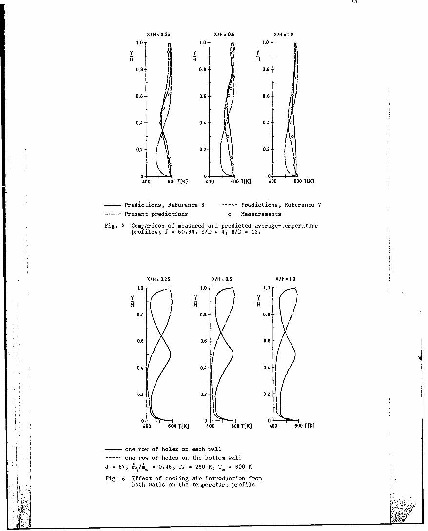
7-7

XIH 0.25 X/H 0.5 X/H 1.0

1.0 1.0 - 1.0

y y I; yH H I. H

0.8-- 0.8- 0.8-

- 0.6-- 0.6- <

II/I. I.)

0.4 0.4 " 0.4 V,

0.2 - 0.2 0.21 o

0., 01 0! '400 600 T[K] 400 600 TIK] 400 600 T[K]

Predictions, Reference 6 Predictions, Reference 7

.... Present predictions 0 Measurements

Fig. 5 Comparison of measured and predicted average-temperatureprofiles; J 60.34, S/D 4, H/D 12.

XlH 0.25 X/H 0.5 XIH 1.0

1.0 - . 1.0 . yl.0 -

HH H/0.8- / 0.8- / 0.8- /

0.6 0.60-- 0.6--

0.44 0.4 .

0.2 0.2 -0.2-

0 0 0400 600 TEKI 400 600 T[K] 400 600 T[K)

one row of holes on each wall

----- one row of holes on the bottom wall

57, ;t/A = 0.48, Tj 290 K, T. = 600 K

Fig. a Effect of cooling air introduction from

both walls on the temperature profile

1 I

4. CONCLUSIONS

The present prediction procedure for the calculation of the average radial tempera-ture profiles in annular combustors was compared with experimental measurements and withtwo different jet mixing correlations. Despite the crude assumption of two-dimensionalflow, the agreement between predicted temperature profiles and the measurements is suf-ficient, for use as a preliminary design tool for complex geometries as originally in-tended. Although the jet mixing correlations give better predictions of those measurementsfrom which they were developed - as expected - the present procedure represents a betterdesign technique; as it can be easily developed to include the effects of heat transferwith the combustor outer casing, the converging combustor exit (turbine inlet), theeffects of film-cooling and opposite-wall cooling-air injection. The use as a design toolto show the effects of changing the design parameters of the combustor seems to bear con-siderable advantages. The final design decission, however, should be based on a more de-tailed analysis, i.e. three-dimensional calculation. Presently detailed experimentalstudies are under way for a verification of two-dimensional and three-dimensional codesunder hot gas conditions.

REFERENCES

1. Lefebvre, A.H. The Design of Tubular Gas Turbine Combustion Chambers forNorster, E.R. Optimum Mixing Performance.

Proc.Insitution of Mech.Engrs., Vol.183, p.150, 1968.

2. Norgen, C.T. Dilution Jet Mixing Study for Gas Turbine Combustors.

Humenik, F.M. NASA TN D-4695, 1968.

3. Walker, R.E. Multiple Jet Study.Kors, D.L. NASA CR-121217, 1973.

4. Holdeman, J.D. Mixing of Multiple Dilution Jets with a Hot PrimaryWalker, R.E. Airstream for Gas Turbine Combustors.Kors, D.L. AIAA Paper 73-1249, Las Vegas, Nev., 1973.

5. Walker, R.E. Multiple Jet Study Data Correlations.Eberhardt, R.G. NASA CR 134795, June, 1975.

6. Cox, J.B., Jr. Multiple Jet Correlations for Gas Turbine Engine CombustorDesign.ASME Paper 75-GT-45, Houston, Tex., 1975.

7. Holdeman, J.D. Mixing of a Row of Jets with a Confined Crossflow.Walker, R.E. AIAA Journal, Vol.15, p.243, Feb., 1977.

8. Spalding, D.B. Basic Equations of Fluid Mechanics and Heat and Mas&Transfer and Procedures for Their Solution.Report HTS/76/6, Imperial College, London, 1976.

9. Elghobashi, S. Unsteady Combustion of Fuels in Jet Engine Afterburners.Pratt, D.T. Third International Symposium on Air Breathing Engines,Spalding, D.B. DGLR-Fachband Nr.6, Munich, 1976.Srivatsa, S.K.

10. Launder, B.E. The Numerical Computation of Turbulent Flows.Spalding, D.B. Computer Methods in Applied Mechanics and Engineering,

Vol.3, p.269, 1974.11. Khalil, E.E. The Calculation of Local Flow Properties in Two-Dimensional

Spalding, D.B. Furnaces.

Whitelaw, J.H. Int.J. of Heat and Mass Transfer, Vol.18, p.775, 1975.

12. Caretto, L.S. Two Calculation Procedures for Steady, Three-DimensionalGosman, A.D. Flows with Recirculation.Patankar, S.V. Proceedings of the Third Int. Conference on NumericalSpalding, D.B. Methods in Fluid Mechanics, Vol.II, p.60, 1973.

13. Wittig, S.L.K. Zum EinfluA der Mischzone auf die TemperaturprofilentwicklungElbahar, 0. am Austritt von Gasturbinenbrennkammern.Festschrift zum 70. Geburtstag von Prof. R. Friedrich,Universit~t Karlsruhe, p.131, 1979.

!4ACKNOWLEDGEMENTS

Thanks are due to Dr. D. Hennecke and Dr. B. Simon, Motoren- und Turbinen-Union(MTU) Mlnchen, for their helpful discussions.

7-9

DISCUSSION

J.McGuirk, UKI would like to comment on your explanation of the fact that your predicted minimum temperature is closer to theinjection wall than was measured. I think your reasoning, which highlighted the physical differences between 2Dcalculatioas and 3D measurements, may be correct, but even if you compared with proper 2D (plane) measurements,I think you would discover the same discrepancy. Calculations we have made at Imperial Collage for only 2D(i.e. plane) slot jets in cross flow show that, particularly for the high momentum flux ratios you are considering, therecirculation length downstream of injection is too short, hence the jet trajectory curves too quickly back to theinjection plane, and the same discrepancy as you observe is obtained.

Author's ReplyYour comment is quite true. Earlier today we have seen similar effects for more detailed calculations. We feel wecan introduce simple correction terms to account for this effect. However, this is an inadequate procecure and wepreferred to present the uncorrected results for comparison. The basic problem - and you certainly have a betterfeeling for it than we do - probably stems from the turbulence model. In our experimental study we are planningto i.nvstigate thib point in more detail.

P.Magre, FrCan you predict the effects of the inhomogeneities at the exit of the primary zone on the temperature profile at theexit of the burner.

Author's ReplyThe computer program is certainly able to account for i.on-homogeneous flow and temperature distributions.However, they must be specified as boundary conditions at the inlet plane into the mixing zone.

As I already mentioned, we have not yet incorporated detailed primary zone calculations discussed earlier today intothe present version of the computer program.

D.C.Dryburgh, UKExperience with practical combustors indicates that there are large random effects in the dilution zone. Why theseshould exist is not known with certainty but it may be due to utstable flows in the annulus feeding of the dilutionholes, to manufacturing tolerances and irregularities in the dilution holes and so on. This appears to imply thatprogress will require the use of fundamental models - possibly of finite difference type - and that to understandthe random effects we may have to consider regions with 2 or 3 jets, rather than a region with half a jet and half aspace with symmetry conditions. Could the author comment on this viewpoint?

Author's ReplyI agree basically with your assessment of the general problem. These questions were actually one of the dominantreasons for us to initiate the present study. We were iiiterested in evaluating the effects of various parameters, i.e.wall temperature, momentum flux ratio, no,.-symmetric jet arrangement etc. At present, however, our program willnot be applicable to unsteady mixing flows. These will be considered later. The present goal is to check on thelimitations of available correlations and to provide the designer with a relatively simple tool in developing acombustor.

A.Sotheran, UKI just make a point that I think practical. Randomness begins in the compressor, and in the diffuser. You .ust triedto find it in the dilution zone. These are more realist models than all of them with CO, NOx predictions in theprimary zone.

Author's ReplyI agree.

I0

7.9

DISCUSSION

J.McGuirk, UKI would like to comment on your explanation of the fact that your predicted minimum temperature is closer to theinjection wall than was measured. I think your reasoning, which highlighted the physical differences between 2Dcalculations and 3D measurements, may be correct, but even if you compared with proper 2D (plane) measurements,I think you would discover the same discrepancy. Calculations we have made at Imperial College for only 2D(i.e. plane) slot jets in cross flow show that, particularly for the high momentum flux ratios you are considering, therecirculation length downsteam of injection is too short, hence the jet trajectory curves too quickly lack to theinjection plane, and the same discrepancy as you observe is obtained.

Author's ReplyYour comment is quite true. Earlier today we have seen similar effects for more detailed calculations. We feel wecan introduce simple correction terms to account for this effect.. However, this is an inadequate procecure and wepreferred to present the uncorrected results for comparison. The basic problem - and you certainly have a betterfeeling for it than we do - probably stems from the turbulence model. In our experimental study we are planningto invcstigate ti point in more detail.

P.Magre, FrCan you prcdict the effects of the inhomogeneities at the exit of the primary zone on the temperature profile at theexit of the burner.

Author's ReplyThe computer program is certainly able to account '-r non-homogeneous flow and temperature distributions.However, they must be specified as boundary conditions at the inlet plane into the mixing zone.As I already mentioned, we have not yet incorporated detailed primary zone calculations discussed earlier today intothe present version of the computer program.

D.C.Dryburgh, UKExperience with practical combustors indicates that there are large random effects in the dilution zone. Why theseshould exist is not known with certainty but it may be due to ui, stable flows in the annulus feeding of the dilutionholes, to manufacturing tolenmces and irregularities in the dilution holes and so on. This appears to imply thatprogress will require the use of fundamental models - possibly of finite difference type - and that to understandthe random effects we may have to consider regions with 2 or 3 jets, rather than a region with half a jet and half aspace with symmetry conditions. Could the author comment on this viewpoint?

Author's ReplyI agree basically wit-i your assessment of the general problem. These questions were actually one of tae dominantreasons for us to initiate the present study. We were interested ir, evaluating the effects of various parameters, i.e.wall temperature, momentum flux ratio, non-symmetric jet arrangement etc. At present, however, our program willnot be applicable to unsteady mixing flows. Thee will be considered later. The present goal is to check on thelimitations of available correlations and to provide the designer with a relatively simple tool in developing acombustor.

A.Sotheran, UKI just make a point that I think practical. Randomness begins in the compressor, and in the diffuser. You just triedto find it in the dilution zone. These are more realist models than all of them with CO, NOx predictions in theprimary zone.

Author's ReplyI agree.

i

9-l

SECOND-ORDER CLOSURE MODELING OF TURBULENTMIXING AND REACTING FLOWS

Ashok K. VarmaGuido Sandri

Coleman duP. Donaldson

Aeronautical Research Associates of Princeton, Inc.50 Washington Road

Princeton, N.J. 08540

Models for the scalar probability density function (pdf) have to be developed toachieve closure of turbulent transport equations for mixing and reacting flows. Adelta function "typical eddy" model has been developed for the joint pdf of the scalar%ariables. It has been demonstrated that delta functions are a necessary part of pdf'sin order to attain the extremums of the statistical constraints on the moments. Thestatistical bounds on a number of moments of interest for two and three species flowshave been derived. It has been proven that a rational pdf composed of a set of deltafunctions alone can always be constructed at any point within the statistically validmoment space. The model provides a good representation of actual pdf's in two-species,variable-density mixing flows. The model has been directly compared to experimentalpdf measurements and good agreement for higher-order moments has been demonstrated. Itcan be shown that the delta function pdf model is significantly simpler than otherproposed pdf models and is more than adequaLe for the closure of the transport equations.

NOMENCLATURE

f, g arbitrary variablesl{ arbitrary functionp pressureP' Pl' P2 probability functionsR universal gas constantT temperatureu flow velocityWa, W, W molecular weights of speciesx coordinate in flow directiony coordinate normal to flow direction

Greek Symbols

c, 8, y species mass fractions3model parameter

63(a-X) delta function located at eA I -1

cell sizes in "typical eddy" modelni entropy of mixingImodel parameter

arbitrary constantp densityp, normalized density

Superscripts

-,1<> time average

fluctuation about mean value

INTRODUCTION

Mixing and chemical reactions under turbulent flow conditions are a basic feature ofthe energy release processes in gas turbine combustors and other propulsion systems, andany predictive modeling of the flowfield has to properly account for the effects of theturbulence of the flow and its interactions with various physical and chemical processes.There are significant interaction effects of the turbulence on combustion and of thecombustion on the turbulence, which are important in determining combustion efficiency,pollutant formation, combustion noise, heat transfer, etc. Second-order closure modelingof turbulent flows provides a convenient framework foi studying these interactions andholds promise of providing a reliable predic-ive computational tool Zor the design ofInew systems and improvement of existing combustion systems.

The presence of finite-rate chemicaL reactions in a turbulent flow introduces theproblem of prcper modeling of many higher-order correlations involving scalar variablessuch as concentration, density and temperature. The transport equations for the meanvariables and the second-order correlations are solved in a second-order closure procedureand these equations and especially the chemical reaction source terms contain many third--rder and higher-order correlations, such as 77, F7c, 1 , etc. These correlations haveto be modeled in terms cf the lower-order moments to close the system of transportV - " equations. A couvenipnt procedure for modeling these scalar cirrelations i3 to model or

calculate the probability density function (pdf) for the scalars. This procedure isbeing used at A.R.A.P., as well as by Rhodes, et al., (1) Bray and Moss, (2) Lockwood andNaguib (3), Libby (4), Bonniot (5) and Kewley (6).

A number of the above approaches require a number of simplifying assumptions ;nddeal only with one-dimensional pdf's. Most of them are also restricted to fast chemistryand cannbr handle finite-rate chemical reactions. The A.R.A.P. model, called the deltafunction "typical eddy" model is designed to be applicable to finite rate chemicalreactions and models the joint pdf for all the scalars in a turbulent reacting flow. Thebasic model has been discussed by Donaldson (7) and Donaldson and Varma (8). Kewley (6)is using the A.R.A.P. model with some modifications and has reported good results onmodeling of reacting flows.

Efforts are also being made to avoid the assumptions regarding the shape of the pdf,by directly solving transport equations for the pdf (9, 10, 11), However, these equationshave only been solved for very simple flowfields and there appear to be serious modelingproblems for some of the terms in the equations. Spalding (12) has recently proposed analternate approach that involves the calculation of the pdf by following the age historyof various eddies.

The paper discusses the statistical behavior of scalar variables in turbulent flows.Constraints on two and three species systems have been derived. The delta function"typical eddy" pdf model has been carefully tested against pdf measurements in a two-species, variable-density mixing layer and good results have been obtained,

STATISTICAL CONSTRAINTS ON CORRELATIONS

Basic statistical principles can be used to develop a set of constraint conditionson correlations of various variables in a turbulent flowfield. The procedure is quitegeneral and can be applied to scalar or vector variables, but at the present time, we aremainly interested in the constraints on scalar moments--specifically those for the thespecies mass and/or molar concentration variables.

The constraint conditions are useful in a number of ways. The statistical constraintson first and second-order correlations are important in the question of "realizability"of second-order closure turbulence models. The lower-order moments are calculated by thesolution of a set of modeled partial differential equations. It is possible that themodeled equations may not have solutions that are consistent with the independentlyderived statistical constraints, andthis will require appropriate corrections to the modelsused in the equations. The statistical constraints on the third-order and higher-ordermoments are also useful in formulating models for these correlations. They are also usefulin determining model sensitivity and the error-bounds of the modeling procedure.

BASIC THEOREMS

Cauchy-Schwarz Inequality

The statistical constraints on various moments of the fluctuations are basicallyderived from conservation conditions and the Cauchy-Schwarz inequality. The Cauchy-Schwarz condition for arbitrary variables f and g is

F7 a. T'> (1)

The equality holds if and only if,

f = Xg (2)

In principle, with suitable choices of f and g, one can derive all the requiredstatistical constraints. In practice, this is not easy. A very useful short-cut is theuse of a "Renormalizatio _orem. Xf we have proven that,

0f2 (A)P!(I A Z(A)dA A >d ! gPl (A)d A )

JO0

then it can be proven that for H(A) > 0

Hf2(A)PI(A)dA Hg2(A)PI(A)dA ( HfgPI(A)dA (4)

The proof is simple. Since Eqn. 3 is valid for all P one can select P1 of thespecial form HP, for any P Then Eqn. 4 follows. Note tAat the reverse passage ftomEqn. 4 to Eqn. is not vaiid in general.

Two other inequalities are useful.

Jensen's Inequality

If f(a) is convex (f" > 0 throughout the domain of interest, 0 < a < 1) then,

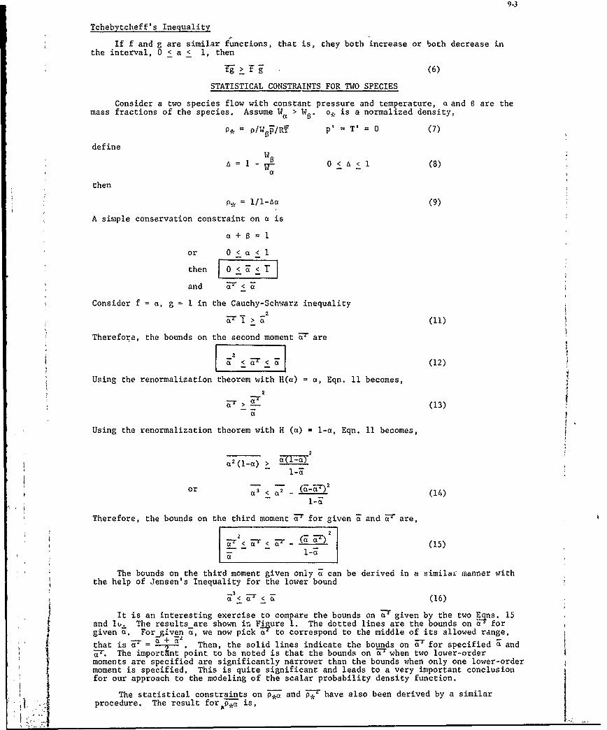
9-3

Tchebytcheff' s Inequality

If f and g are similar functions, that is, they both increase or both decrease inthe interval, 0 < a < 1, then

Fr (6)

STATISTICAL CONSTRAINTS FOR TWO SPECIES

Consider a two species flow with constant pressure and temperature, a and 6 are themass fractions of the species. Assume Wa > WB . o. is a normalized density,

P.= P/Wa /RT p' = T' = 0 (7)

defineW8

A= - 0 < l (8)a

then

= I/l-LAa (9)

A simple conservation constraint on a is

a +=i

or 0<a<l

then 0 < 3 < T

and U <

Consider f = a, g 1 in the Cauchy-Schwarz inequality2 (ll

Therefore, the bounds on the second moment W- are

a < Tr< (12)

Using the renormalization theorem with 11(a) a, Eqn. 11 becomes,

2

- (13)

Using the renormalization theorem with H (a) = 1-a, Eqn. 11 becomes,

2

a 2( -a) > a-a

or a < a- (_ T)2 (14)

Therefore, the bounds on the third moment ' for given - and 37 are,

1-01< 3 -< 7T) (15)

The bounds on the third moment given only a can be derived in a similar manner withthe help of Jensen's Inequality for the lower bound

33 < U7 < Z (16)

It is an interesting exercise to compare the bounds on 3T given by the two Eqns. 15

and lu. The results-are shown ir. Fjure 1. The dotted lines are the bounds on a forgiven a. For given a, we now pick a to correspond to the middle of its allowed range,

that is a + .* Then, the solid lines indicate the bounds on U- for specified a andT*The impotn point to be noted is that the bounds on 7~ when two lower-order

moments are specified are significantly narrower than the bounds when only one lower-ordermoment is specified. This is quite significant and leads to a very important conclusionfor our approach to the modeling of the scalar probability density function.

The statistical constraints on -- and have also been derived by a similarprocedure. The result for -- is,

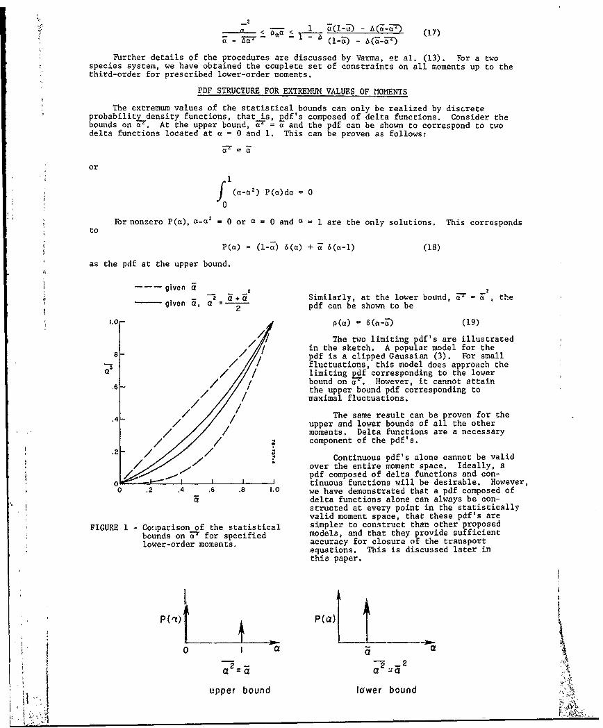
- -l 1- - A(a-"TO (17)< < (1-) -

Further details of the procedures are discussed by Varma, et al. (13). For a twospecies system, we have obtained the complete set of constraints on all moments up to thethird-order for prescribed lower-order moments.

PDF STRUCTURE FOR EXTREMUM VALUES OF MOMENTS

The extremum values of the statistical bounds can only be realized by discreteprobabilitydensity functions, that is, pdf's composed of delta functions. Consider thebounds on 3i. At the upper bound, 3' = a and the pdf can be shown to correspond to twodelta functions located at a = 0 and 1. This can be proven as follows:

or

J (a_ 2 ) P(a)da = 0

0

Ibr nonzero P(c), c-c 2 = 0 or a = 0 and a = I are the only solutions. This corresponds

to

P(a) = (1-a) 6(a) + i 6( -I) (18)

as the pdf at the upper bound.

---- given a 22 a + a Similarly, at the lower bound, W , the

- given a, a pdf can be shown to be~2

I.0- P(a) = 6(ct-D) (19)

The two limiting pdf's are illustratedin the sketch. A popular model for the

- pdf is a clipped Gaussian (3). For small-/ / fluctuations, this model does approach the

a / limiting pdf corresponding to te lowerbound on c-. However, it cannot attain

6/ / the upper bound pdf corresponding to/ / maximal fluctuations./ /

4The same result can be proven for the.4- / upper and lower bounds of all the other// moments. Delta functions are a necessary

// = component of the pdf's.

.2- / / Continuous pdf's alone cannot be valid

/ over the entire moment space. Ideally, apdf composed of delta functions and con-

0 I tinuous functions will be desirable. However,0 .2 .4 .6 .8 1.0 we have demonstrated that a pdf composed of

delta functions alone can always be con-structed at every point in the statisticallyvalid moment space, that these pdf's are

FIGURE I - Conparison of the statistical simpler to construct than other proposed

bounds on W- for specified models, and that they provide sufficientlower-order moments. accuracy for closure of the transport

equations. This is discussed later inthis paper.

upper bound lower bound 'N'

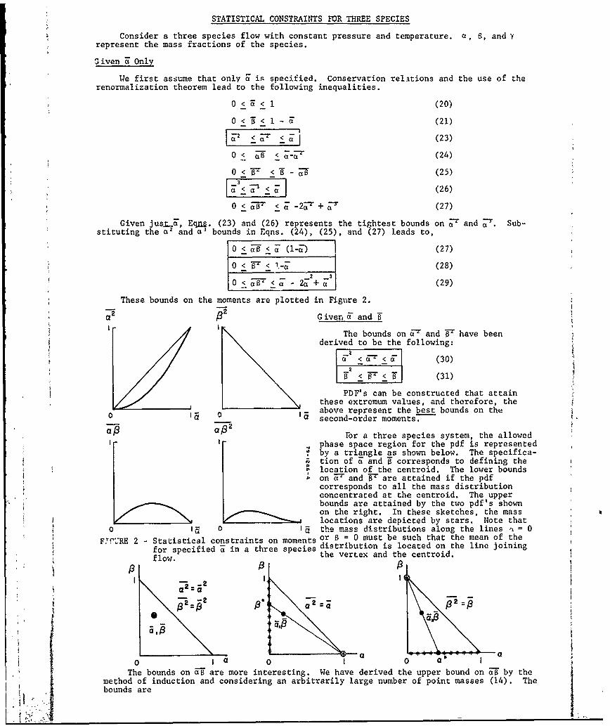
STATISTICAL CONSTRAINTS FOR THREE SPECIES

Consider a three species flow with constant pressure and temperature. a, 8, and yrepresent the mass fractions of the species.

Given F Only

Ile first assume that only & is specified. Conservation relations and the use of therenormalization theorem lead to the following inequalities.

0 < 'a < 1 (20)

0 < "9 < 1 (21)

a2 < - <- (23)

0 < 8 < aa-r (24)

0 < 7 < - (25)

a < 7< a ](26)

0 < T < a- -2a- - +- (27)

Given jus .r_., Equ . (23) and (26) represents the tightest bounds on 7 and a'. Sub-*stituting the a2 and a' bounds in Eqns. (24), (25), and (27) leads to,

0 <T<a (- - (27)

0 < F < (28)

_77 a- 2 + (29)

These bounds on the moments are plotted in Figure 2.

a2 / Giver " and

The bounds on 6" and F have beenderived to be the following:

< -< (30)

2

<j < (31)

PDF's can be constructed that attainthese extremum values, and therefore, theabove represent the best bounds on the

0o 0 IQ second-order moments.

For a three species system, the allowedphase space region for the pdf is representedby a triangle as shown below. The specifica-tion of - and T corresponds to defining thelocation of the centroid. The lower boundson Z7 and - are attained if the pdfcorresponds to all the mass distributionconcentrated at the centroid. The upperbounds are attained by the two pdf's shownon the right. In these sketches, the masslocations are depicted by stars. Note that

o 0 I the mass distributions along the lines =0FIGURE 2 -Statistical constraints on moments or 8

= 0 must be such that the mean of the

for specified U in a three species distribution is located on the line joiningfo.the vertex and the centroid.~flow.

0 1 a 0 0 a

The bounds on F are more interesting. We have derived the upper bound on i!W by the

method of induction and considering an arbitrarily large number of point masses (14). Thebounds are

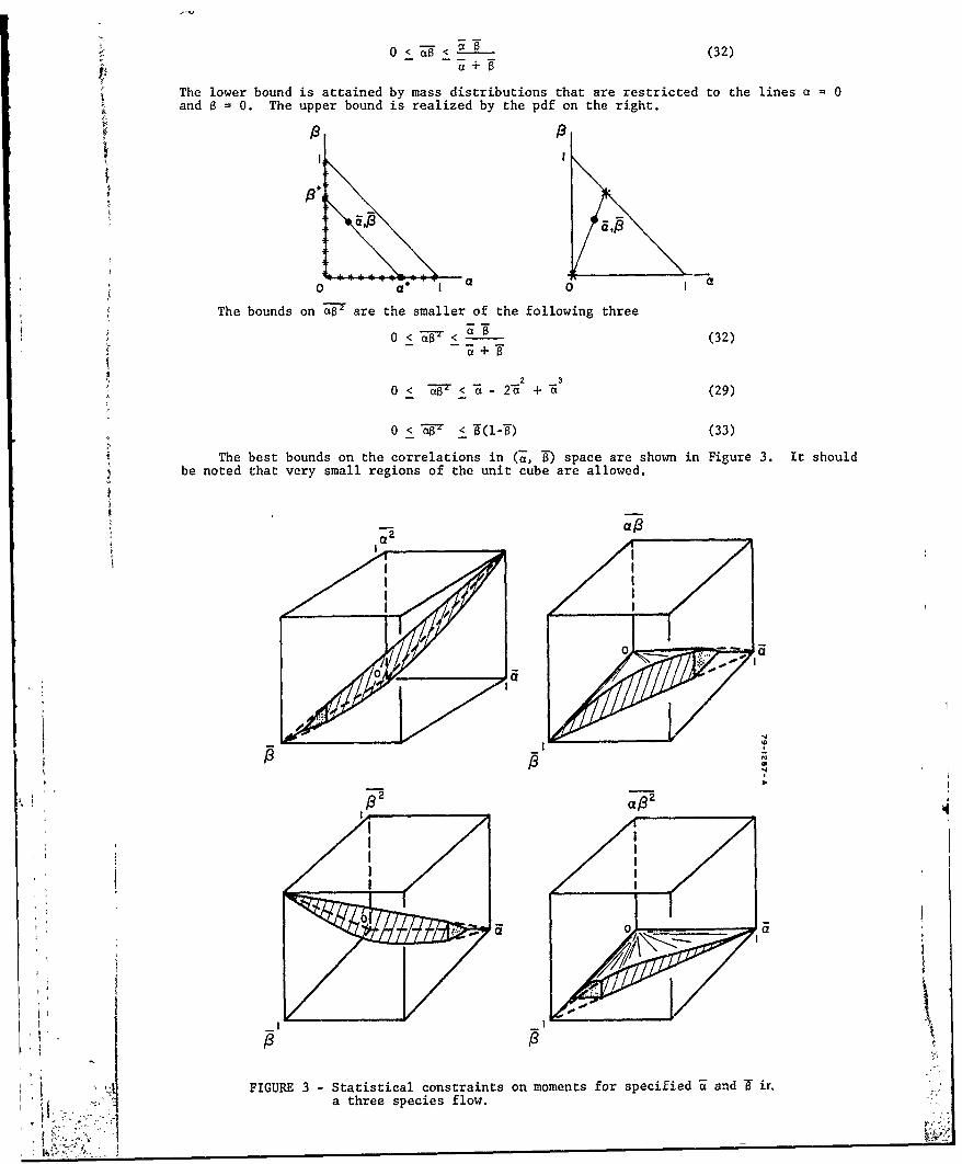
0< 7 < (32)-a+

The lower bound is attained by mass distributions that are restricted to the lines a =0and 6 = 0. The upper bound is realized by the pdf on the right.

0 - l

The bounds on a are the smaller of the following three_ (32)

2 30< <-'a - 2* +'7 (29)

,0 < -08 < W(I-T") (33)

The best bounds on the correlations in (-, T) space are shown in Figure 3. It shouldbe noted that very small regions of the unit cube are allowed.

p ,

a2a

_1 2

FIGURE 3 " Statistical constraints on moments for specified U and T r.a three species flow.

Given 3, W, and 3-

Fclowing very similar procedures, we have determined the allowed regions for -,- and 70" in 77 space for specified E and B. The procedure is illustrated below byone example; further details are available in (14).

The independent bounds on 3r and WT (Eqns. 30, 31) define a rectangle in (W, -)space. However, there are regions within the rectangle that must be excluded. Similarly,there are excluded regions in (71, 7) and (-7, 78) spaces.

2

Consider 3-7 a

The minimal value of 71 is attained by the following distribution.

8T2 foBP,()dB ,

00

: BConsider p2(= dB

For simplicity, consider P2(B) to be a two delta function distribution with the deltafunctions located on the sides of the triangle (sketch below).

! g =w(l -a) Wi o1

It~~~ ispsuae'hta34)

It ispotulated tha cannot be larger than this value for other general massdistributi~ns P2(0) that are located in the interior region of the triangle. Similarly,for ,the largest allowed 71 is

37= F(1 - ) (35)

Using the general distribution,

-= faB 6 (a -) P2 (B) dBda

= (36)

Similarly, a--'' '- 2 '

The allowed values of W- range from T to g(l-E) and therefore,

8 < a- < (a-) (37)

The allowed bounds on the correlations for other limiting values of Wz, , etc.,have been similarly calculated. The shapes of the connecting curves between the allowedpoints have been determined by considerin& a series of two delta function pdf's, with the

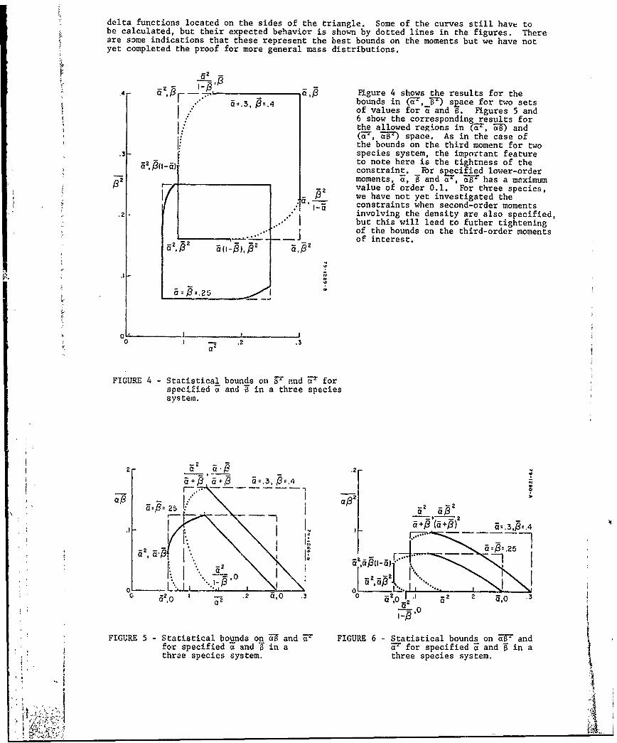
delta functions located on the sides of the triangle. Some of the curves still have tobe calculated, but their expected behavior is shown by dotted lines in the figures. Thereare some indications that these represent the best bounds on the moments but we have notyet completed the proof for more general mass distributions.

-2a13

.4- 332,rF , Figure 4 shows the results for thea-.3, R.4 bounds in (7-, -r) space for two sets

S.of values for - and 8. Figures 5 andI! 6 show the corresponding results for

the allowed regions in (3E, Z) and(-r, -- ) space. As in the case of[. the bounds on the third moment for two

.3 species system, the impovr'ant feature-2 (_ to note here is the tightness of the

constraint. Fbr specified lower-order2 moments, and -, 7 has a maximum

1 -- 2 value of order 0.1. For three species,a,-13 we have not yet investigated the

:j." l-a constraints when second-order moments.2 involving the density are also specified,7 .'"but this will lead to futher tightening

of the bounds on the third-order moments.... . ."'--- of interest.

0 ,I - .2 .3

. a1

FIGURE 4 - Statistical bounds on a Pnd T' forspecified and 7 in a three speciessystem.

o +' c 3, "rS 0 .-.2 , , e 2 ,0 .

0

FIGUR 5 a F2 -2

25 132~

F he ei esyt, threeI~f spcis ysem

+ 02 a .0.2

-- a

j0

COMPARISON OF "TYPICAL EDDY" MODEL WITH PDF MEASUREMENTS

The "typical eddy" model is an attempt to define the joint pdf for the scalarvariables by using all the available information from a second-order closure analysis.The model may consist of combinations of delta functions and continuous functions but wehave extensively studied a model composed of delta functions alone. The model parametersare determined by matching the moments of the model to the values of the correlationsobtained from the solution of the transport equations. The procedure is detailed in (13).

In a two-species, variable density flow, the pdf model consists of 4 delta functions.The model has one free parameter, designated a3, and we have demonstrated (13) that theallowed range of a 3 corresponds directly to the statistical bounds on the third-ordermoments wr or --F . With the parameter a selected at any point within its allowed range,we have also shown that a physically correct pdf model composed solely of delta functionscan be constructed at every point in the statistically valid moment space. We will nowdemonstrate that these models provide sufficient accuracy for closure of the transportequations for turbulent flows.

Comparison with Experiments

Konrad (15) has made a series of detailed measurements of the pdf in three shearlayer flowfields. The measurements have been made in (i) a He-N, shear layer with avelocity ratio u /u = 0.38 and a density ratio P2 /p, = 7.0. (ii a uniform densityHe+Ar-N2 shear liye with velocity ratio of u2/u = 1.38 and (iii) a wake flow in whichthe gases have equal free-stream velocities and a density ratio of 7. All the flows arelow speed and two-dimensional. The measurements consist of mean velocity, mean concen-tration, concentration fluctuation correlations, species intermittency functions and thespecies pdf's. The latter two parameters are used for the direct model comparison. Onlythe results for the first flowfield are discussed in this paper. Further studies andcomparisons are available in (13).

The pdf measurements are used to determine the values of the four lower-order moments--, .-, !p and p --that are needed to construct the two-species variable-density "typicaleddy" model. The measured pdf is also used to calculate experimental values of a numberof third-order correlations of interest, such as 7$' and a 8. The third-order momentsare also computed from the model and the results compared Lo the measurements. The validrange of the free parameter a., corresponds to the upper and lower bounds on the thirdmoments.

Figure 7 presents the results for the third moment 3-' for the He-.N3 shear layer. Theordinate of the figure is F-B model /- expt. The abscissa is the normalized coordinate

across the shear layer. The dotted lines show the upper and lower bounds on the thirdmoment when only two lower-order moments are used for the model construction. In thiscase -- model has a large range of possible values and some models within the statistical

range can lead to significant errors compared to the experiments. However, when 4 lower-order moments are specified, the model values of To' are tightly constrained as shown bythe solid lines. For the "typical eddy" model, the solid lines correspond to the entirevalid range of the parameter a 3 It can be seen that with any choice of a3 within thisrange, it is possible to predict 761 (and other third-order moments) to better than 10%accuracy. This is significantly better accuracy than the expected error bounds onexperimental measurements of third-order moments. Further, such accuracy is expected tobe quite adequate for closure of the transport equations for the means and second-ordercorrelations.

It must be noted that the statistical constraints on the moments are independentof the pdf model. The "typical eddy" model with end-choices of the parameter a3 matchesthe bounds on the third moment. Any and all statistically valid pdf models that match

the given values tor the lower order moments will predict values for the third momentwithin these same bounds. These other modeIs will typically be more difficult to constructand may not lead to significantly better prediction of third-order moments. Betteraccuracy in the prediction of third-order moments does not appear to be necessary as faras closure of the equations is concerned. The delta function "typical eddy" model can beused to provide better accuracy by empirically selecting the parameter a at the middleof its ailowed range, as shown in the figure. The third moment can now be predicted tobetter than 2% accuracy across the entire flowfield.

Konrad has also measured the species intermittency function or the probability offinding pure species at various points across the flowfield. A comparison of the modelpredictions to the data is shown in Figures 8 and 9. The theoretical predictions use acutoff value of 0.9, that is, a delta function located at a > 0.9 is considered to be purespecies a. This is an arbitrary, but reasonable criterion. The results in Figure 8 arefor al equal to the maximum value within its allowed range. This also corresponds to apdf sructure with minimum mixedness or minimum entropy of mixing. The entropy of mixingis defined as,

Fiur 9 shw thei reut -nia _ii npi)

igure 9 shows the results for a at midrange and a3 equal to the minimum value allowed.It is clear that the empirical cAoice of a maximum leads to significantly better agreement

with the experimental data. Further arguments in support of this choice of a3 thatcorresponds to minimum entropy of mixing are discussed in (13). A qualitative com-

, parison of the delta function pdf for maximum a, and the measured pdf is shown in

1.6 2

A ate).1:~?u/ 1 03

A -- N -

1. 2.

17

/

/'/ - -- -- a, a- specified

,,'8/ a, a , pa, p: specified! - - -- =" ,pa,p' 3pecified, ;,

' 3 at midiangei- 1I I I0 .06

! y/(X- o)FIGURE 7 . Comparison of model predictions and experiments for the

third moment a-8. He-N2 shear layer.

~~~~~ .I.. Typca Edypde Pedctone 8

Tyia Ed.od!PedcinTypical Eddy Model Predictionsz - 3 maximum 2 - at midrange

S. - - -- minimum

0. a.

= .{ I u,/u s.36 =5\ 2 L~ ~ u/~03

thr moet(FHe)2sha lyr

"- . 0 Konrod data -- .2 - o Konrad data

Li .8

0o 0

Q. maiu a3a .dag

.0.0

0) X4)N )

.- .6 .= .6

S. 0.u& .6 (

,,- 0 - -

.S .4 .-.4 X

.2 /a

0 .0

0. i 0 0. oi" ,-- 0 o I

00

S.42 --0 0 E0 .- 2 -00.6

t y/(x x o )y/(x-Xo

i FIGURE 8 - Comparison of model predictions F'igure 9 - Comparison of model predictions with ,with experiments for the probability of experiments for the probability of finding pure !finding pure species. a3 maximum model. species. a3 at midrange and a3 minimum models.

-t - He-N2 shear layer. He-N2 shear layer.

.06

4- -.06

0

0 12 u2/u= 0.380 2 . .6 .8 1.0 p21= 7.0

C(He) a3 maximum model

Probability density functions

FIGURE 10 - Comparison of delta function pdf with measured pdf.

Figure 10. The experimental pdf is reproduced from the report by Konrad (15). The deltafunctions in the model are shown at their correct locations in the concentration space andthe relative strengths of the delta functions are correct. The absolute magnitude of thestrength of the delta functions cannot be directly plotted on this graph and we haveselected a convenient scale for depicting the delta functions. The delta functionrepresentation of the pdf seems to be capable of capturing the important features of theexperimental pdf structure.

This limited comparison with detailed pdf measurements indicates that the choice ofa3 maximum shows the best overall agreement with data for a two species variable densitymixing flow. It will be desirable to compare the model to other data for different flowconditions for further model evaluation. Further, similar comparisons of the model forthree species to measurementa in simple reacting flows have to be carried out. However,it appears that the delta function pdf model is capable of predicting higher-order momentsto sufficient accuracy for closure of the transport equations.

CONCLUSIONS

The direct comparison of the delta function "typical eddy" model for two species withpdf measurements has demonstrated that this simple model is quite adequate for achievingclosure of the transport equations. The complete set of statistical constraints oncorrelations for two species flows have been derived. The constraints have been used toprove that delta functions are a necessary part of pdf in order to attain the extremumvalues of the moments. A rational pdf composed of a set of delta functions alone canalways be constructed anywhere within the statistically valid moment space. A pdf ofthis type when constructed using all the available information in a second-order closurecalculation, can predict higher order correlations to an accuracy better than they can bemeasured. It, therefore, appears unnecessary to construct more complex pdf's for thepurpose of closure of the turbulence equations.

A number of the important statistical coustraints for three species systems have beenderived, and these indicate that the third-order correlations are quite tightly constrained.Therefore, it appears likely that the conclusions arrived at for two species mixing flowswill also be applicable co simple reacting flows.

REFERENCES

1. Rhodes, R.P., Harsha, P.1., and Peters, C.E.: Turbulent Kinetic Energy Analyses ofHydrogen-Air Diffusion names. Acta Astronautica, Vol. 1, 1974, pp. 443-70.

2. Bra), K.N.C. and Moss, J.B., thiversity of Southhampton, "A Uified Statistical Modelof the Premixed Turbulent Flame, 1974, AASU Report No. 335.

3. Lockwood, F.C. and Naguib, A.S., The Prediction of the Fluctuations in the Properties

of Free, Round-Jet, Turbulent, Diffusion Flames, Combustion and fame, Vol. 24,1975, p. 109.

4. Libby, P.A., On Turbulent Flows with Fast Chemical Reactions, III, Two-DimensionalMixing with Highly Dilute Reactants, Combustion Science and Technology (Special Issueon Turbulent Reactive fows), Vol. 13, Nos. 1-6, 1976, pp. 79-98.

5. Bonniot, J.C., Borghi, R., and Magre, P., "Turbulent Combustion in a StirredCombustor," in Turbulent Combustion, Vol. 58, AIAA Progress in Astronautics andAeronautics Series, 1977.

6. Kewley, D.J., Development of a Second-Order Closure Model for Turbulent ReactingFlows, Presented at the 6th Australasian Hydraulics and Fluid Mechanics Conference,December 5-9, 1977, Adelaide, Australia.

7. Donaldson, C. duP., On the Modeling of the Scalar Correlations Necessary to Constructa Second-Order Closure Description of Turbulent Reacting Flows, Turbulent Mixing inNonreactive and Reactive Flows, Plenum Press, New York, 1975, pp.

8. Do..aldson, C. duP. and Varma, A.K., Remarks on the Construction of a Second-OrderClosure Description of Turbulent Reacting Flows, Combustion Science and Technology(Special Issue on Turbulent Reactive Flows), Vol. 13, Nos. 1-6, 1976, pp. 55-78.

9. Dopazo, C. and O'Brien, E.E., Statistical Treatment of Non-Isothermal ChemicalReactions in Turbulence, Combustion Science and Technology (Special Issue onTurbulent Reactive Flows), Vol. 13, Nos. 1-L, 1976, pp. 99-122.

10. Bonniot, J.C. and Borghi, R., Sur la Densite de Probabilite des Fluctuations D'EspecesReactives Dans la Combustion Turbulente, Communication presentee au 6e ColloqueInternational sur la Dynamique des Gas et Explosion et des Systemes Reactifs,August 22-26, 1977, Stockholm, Sweden.

11. Pope, S.B., The Probability Approach to the Modeling of Turbulent Reacting Flows,Combustion and Flame, Vol. 27, 1976, p. 299.

12. Spalding, D.B., A General Theory of Turbulent Combustion, the LaGrangian Aspects,AIAA Paper No. 77-141, 1977.

13. Varma, A.K., Sandri, G., and Mansfield, P.J., A.k.A.P., Inc., 'Modeling of ScalarProbability Density Functions in Turbulent Flows," Project SQUID Technical ReportARAP-l-PU., 1978.

14. Varma, A.K., Mansfield, P.J., and Sandri, G., A.R.A.P., Inc., "Second-order ClosureModeling of Variable Density Turbulent Flows," Project SQUID Technical Report ARAP-2-PU, 1979.

15. Konrad, J.H., Californfi Institute of Technology, An Experimental Investigation ofMixing in Two-Dimensional Turbulent Sh!ear Flows with Applications to Diffusion-Limited Chemical Reactions, Project SQUID Technical Report CIT-8-PU., 1976.

ACKNOWLED3 MENTS

This research effort has been supported by the Office of Naval Research under ContractNos. N0014-75-C-1143 (Project SQUID) and N0014-79-C-0335. Some support from the Air ForceOffice of Scientific Research under Contract No. F44620-76-C-0048 is also gratefullyacknowledged. The authors wish to acknowledge the close involvement of Dr. P.J. Mansfieldin the derivation of the statistical bounds.

E4

9-13

DISCUSSION

N.Peters, GeLet me congratulate you for the systematic investigation of the statistical constraints for higher order moments.However, let me comment that I do not believe that delta-function pdf's will be useful for the calculation of meanreaction rates in combustion situations. Laminar production rates plotted over the mixture fraction or a progressvariable (for instance temperature) peak very sharply close to the stoichiometric mixture and at the upper adiabatictemperature limit. A delta function will give a zero mean reaction rate if it lies out of the peak and the laminarvalue if it falls on it.

Author's Reply

Please also see the reply to the question of Dr Jones.

The strong dependence of the reaction rate on the temperature is well-known and follows from the Arrhenius rateexpression. We are hopeful that our delta function joint pdf model consisting of 7 delta functions for reacting flowswill result in the placement of a number of delta functions in the high temperature end of the temperature spacesand will predict the correct average reaction rate.

W.P.Jones, UKAs I recall the experiments with which you compared your calculations were isothermal - or nearly so. My feelingis that if you were to apply your model to a flame, then the results - in particular the temperature profiles - wouldbe much more sensitive to the selected p.d.f. and that forms constructed from Dirac 6-functions will not beadequate. My reasons for holding this view are that in calculating H2 -air turbulent diffusion flames using variousp.d.f. forms I found that the Dirac 5-function form generated double peaked radial temperature profiles'. Wouldyou like to comment on this result and the implications for your model?

1. Jones, W.P. Turbulence Models for Turbulent Flow with Variable Density and Combustion. Tobe published by Hemisphere Pub. Co., VKI Lecture Series, 1979.

Author's ReplyThe results in the paper demonstrate that the delta function pdf model appears to be adequate for mixing flows.We are now working on extending the pdf model to reacting flows. We are aware of the referenced results ofDr Jones ard are concerned about the problem of greater sensit'vity of reacting flow calculations to the form of thepdf. Fo simple reacting flows involving 3 species our model for the joint pdf of all the scalars will consist of 7 deltafunctions and we are hopeful that this will lead to more satisfactory results. The main argument for the deltafunction model is its simplicity of construction compared to other pdf models but if the model does not provesatisfactory, it is conceptually straight-forward to use our procedure for constructing continuous type joint pdf's.

C.H.Priddin, UKYour model shows clearly how closely the third-order moments are bounded for correlations between species whichare themselves bounded by the values 0 and 1. However, to calculate reaction rates one also needs to evaluatecorrelations involving fluctuating reaction rate or temperature, which are not bounded to such an extent. How canyour model cope with these terms?

Author's ReplyWe are currently examining the constraints on temperature related correlations. Bounds on the temperature variablethat can be used are the initial temperature and the adiabatic flame temperature, and these can be suitablynormalized to range between 0 and 1. We are hopeful that this approach will enable us to derive the desiredconstraints on temperature correlations.

I .

10-I

COMBUSTOR MODELLING FOR SCRAMJET ENGINES

J. Philip Drummond, R. Clayton Rogers, and John S. EvansAerospace Engineers

NASA Langley Research CenterHan,dton, Virginia 23665

U.S.A.

SUMMARY

Combustor flow fields found in hydrogen fueled scramjets are quite complex and, therefore, difficultto analyze. Analyses that adequately model the combustor imust not only consider highly turbulent andreacting flows with complex wave structure, but also must cope with the possibility of embedded subsonicregions and recirculation within a predominantly supersonic flow. Conventional analytic approaches toscramjet analysis and design have been global in nature or have been restricted to all-supersonic flow;they must therefore be extended to realistically describe actual combustor flow fields. A system ofcomputer programs being developed at the NASA Langley Research Center to model these complex combustorflow fields is discussed. Each code solves a system of equations compatible with the type of flow beinganalyzed in any particular part of the combustor. For flows that remain supersonic throughout, a parabolicNavier-Stokes solver is being used successfully. An extension of this computer program, to partially intro-duce elliptic character into the analysis by accounting for a full 3-D pressure field, is being tested.This "partially elliptic" scheme accounts for the effects of streamise pressure feedback present in thesubsonic flow, thereby allowing the detection and calculation of embedded subsonic regions known to bepresent in the combustor. Although the partially elliptic procedure can handle mixed subsonic-supersonicflows, it still requires that a predominant flow direction exists; for recirculating flows, the fully

elliptic Navier-Stokes equations are required. Since recirculating flow does exist in regions near pointsof fuel injection from struts in the engine, work is currently underway to begin development of a three-dimensional elliptic Navier-Stokes solver. Initial work has included development at Langley of a 2-Delliptic code for the analysis of slot fuel injectors. Each computer program is currently being appliedto pertinenc problem areas and is providing a good deal of insight about flow fields in the Langley scramjetengine.

NOMENCLATURE

Ai, Bit Ci reaction rate parameters Pb reference pressure for combustion

A A constants in profile functions data = 2.173 MPaAK, AR m ansin frtiooeffictient q heat flux vectorCf mean skin friction coefficient Ro gas constant

cu mass fraction decay factor R mass flux profile parameterd fuel injector diameter S surface area of control volumed Jet diameter S source function

e stagnation internal energy per unit Sc Schmidt numbervolume T Temperature

es static internal energy per unit t timevolume At time increment

f species mass fraction, streamwise UC0 freestream velocitystretching function or ratio offuel to mainstream flow rate u, v, w, streamwise, transverse andtransverse stretching function or lateral veloity componentsmean square amplitude fluctuations V velocity in TJ modelin species concentrations x, y, z streamise transverse andH stagnation enthalpy latel physical coordinates

H0 molecular w'eighth duct heightKfi reaction rate i, forward direction w species rate of change

YA upper boundary of physical domainKbi reaction rate i, reverse direction lower boundary of physical domaink turbulence kinetic energy YB Z iren n omptaioal

I mixing length AX, AY, AZ increments in computationalLx streamwise finite difference operator finite difference grid

non-dimensional transverse coordi-Ly transverse finite difference operator nate in TJI model

Le Lewis number a numerical damping coefficientM Mach number aB, aT' 'F angles of bottom and topM mole fraction of species j duct walls and jet (fig. 21)M jo, a stretching factors in coo-di-NR number of reactions y nate transformation

r diffusion coefficientS number of species y ratio of specific heats

mainstream mass flow rate y stoichionetric coefficient, forward

y stoichiometric coefficient, backward

Pr Prandtl number ratePi'j stress tensor 6 boundary layer thickness or local

ppressure cflow anglee numerical damping coefficient orI ; p pitot pressure

dissipation rate of turbulencePt jet stagnation pressure kinetic energy

I-I

COMBUSTOR MODELLING FOR SCPAJET ENGINES

J. Philip Drummond, R. Clayton Rogers, and John S. EvansAerospace Engineers

NASA Langley Research CenterHampton, Virginia 23665

U.S.A.

SUMMARY

Combustor flow fields found in hydrogen fueled scramjets are quite complex and, therefore, difficultto analyze. Analyses that adequately model the combustor nijst not only consider highly turbulent andreacting flows with complex wave structure, but also must cope with the possibility of embedded subsonicregions and recirculation within a predominantly supersonic flow. Conventional analytic approaches toscramjet analysis and design have been global in nature or have been restricted to all-supersonic flow;they must therefore be extended to realistically describe actual combustor flow fields. A systeri ofcomputer programs being developed at the NASA Langley Research Center to model these complex cr mbustorflow fleds is discussed. Each code solves a system of equations compatible with the type of ?low beinganalyzed in any particular part of the combustor. For flows that remain supersonic throughout, a parabolicNavier-Stokes solver is being used successfully. An extension of this computer program, to partially intro-duce elliptic character into the analysis by accounting for a full 3-D pressure field, is being tes' d.This "partially elliptic" scheme accounts for the effects of streamwise pressure feedback present in thesubsonic flow, thereby allowing the detection and calculation of embedded subsonic regions know 0 'epresent in the combustor. Although the partially elliptic procedure can handle mixed subsonic-suDersonlcflows, it still requires that a predominant ,'ow direction exists; for recirculating flows, tne fullyelliptic Navier-Stokes equations are required. Since recirculating flow does exist In regions nep' povntsof fuel injection from struts in the engine, work is currently underway to begin development of a tnree-dimensional elliptic Navier-StoPes solver. Initial work has included development at Langley of a Z-Uelliptic code for the analysis of slot fuel injectors. Each computer program is currently being arnlieJto pertinent problem areas and is providing a good deal of insight about flow fields in the Langley scramijetengine.

NOMENCLATURE

Ai , Bit Ci reaction rate parameters Pb reference pressure for combustionAk, AR constants in profile functions data f2.173 a

Zf mean skin friction coefficient R gas cons'nt

cu noss fraction decay factor R mass flux profile parameter

d fuel injector diameter S surface area of control volumed Jet diameter S source function

e stagnation internal energy per unit Sc Schmidt numbervolume T Temnerature

es static internal energy per unit t timevolume At time increment

f species mass fraction, streamwise UC0 freestream velocitystretching function or ratio offuel to mainstream flow rate u, v, w, streamwisc, transverse and

g transverse stretching function or lateral velocity componentsmean square amplitude fluctuations V velocity in TJI modelin species concentrations x, y, z streanwise, transverse and

H° stagnation enthalpy lateral physical coordinatesh duct height W molecular vetghtKt reaction rate i, forward direction species rate of changeKb reaction rate i, reverse d;rection YA upper boundary of physical domaink bturbulence kinetic energy YB lower boundary of physical domain1 mixing length AX, AY, AZ increments in computational

Lx streamwise finite differc operatc'- f-nite difference gridnm.dimensional transverse coordi-L y transvc.Fe finite different orerator nate in TJI model

Le Lewis number 0 numerical damping coefficientM Mach number %8, a179 aF angles of bottom and topN mole fraction of species j duct walls and jet (fig. 21)N B x, 8y stretching factors in coordi-MR number of reactions nate transformationNS number of species r diffusion coefficient

y ratio of specific heatsm0 mainstream mass flow rate y stoichionetric coefficient, forwardni unit normal vector rateyi stoichiometric coefficient, backwardPr Prandtl number rateP stress tensor 6 boundary layer thickness or localp pressure flow angle

ppitot pressure numerical damping coefficient ordissipation rate of turbulencePt,f Jet stagnation pressure kinetic energy

}I

-10-2

mixing parameter £ laminarin mne n valtie, K heat tiansfer coefficient or fuel

hass fraction nnx, nny maximum- grid points in x and yfdirections

I viscosity property behind shockSp density °a normal stress . H0 or stagnationha tesu, v, W, 'o dependent variables

T ~shear stressfk*, @ -general -dependent variable f k, c,t_ W vorticity x, y, z in streamwise, normal or trans-

oIver-relaxation coefficient verse directiondor a w wall- conditionsSbspts6 edge of mixing region where K =0ubscrip dependent,;variable

ci certerl ine -o mai nstreame effective value or exit plane '2 odel plane of TJimodelf fuel jeti, -j, k x, y, and'z grid ihdices or species

'and, reaction indices n, time ,index

1.0 INTRODUCTION,The NASA Langley Research ,Cne is conducting res.rch on a hydrogen fueled sup.rsonic combustion

ramjet :(scramjet) conceptwhth< will be capable of opeiiiing-at hypersonic speeds In the atmosphere. 1

ScramJet perfor;hce ec ,attrctive-atVehicle flight speeds of Mach 4 and above,, and they offer themost viable propulsion :o h piofi h,'h O"'p'a'ltig-at flight.speeds in excess of Mach 6.2 Hypersonic-aircraftconcepts are'being'developc inwhi . 'crimjet is integrated--into the airframe of the vehicle (fig. 1)such that the vehicleitifelf pdtrnis partbfth engine fuofction birlethai precompression and exhaustexpansion while minimiziig the dray associated with the engine. The~engine is divided into several identi-cal'enginie 'modules, one of wh'ich is shown in figure 2. (Th'°7side wall of the module'has been removed to,expos_ the enging's ifitei'nl f eatures.)i The engiie inlet has a varying rectangular cross-section with-fixed geo"'etry. 'Compressl6n is Iiltiated by the Vehicle forebodyahed of the engine; the forebody com-pressesthe flow'vertilally. Each iod Il inlet:;compresses, the flowrhorizontally with swept wedge shapedside walls. The wedges are designed fuch that'thei sweep causes spillage past the cowl of part-of the:inlet air not needed in the low and intermediate Mach number range of operation. Inlet compression iscoilleted by three swept struts, that also provil locations for gaseous hydrngen fuel injection.

Fuel is Introduced into the engine from the strut's in, both a parallel and transverse direction to the-engiie primary flow (fig. 2).' This approach tailors the fuel -injection -to an optimum heat release scheduleover the flight Mach number range-of interest. Transverse fuel injection prom(otes more-rapid -fuel- air-mixingand is used wherever possible to promote reaction in the upstream portion of the combustor. At-'flight Machnumbers below 6, however, too much perpendicular injection results in- thermal choking of the engine. There-fore the parallel injection 'Mde predominates through the low Mach number range of the engine by--slowi.q,the miying and, therefore' stretching-out the reaction process. The flow, having-undergone reaction in 1hecombustr, bpgins to expand in a-shortrn6zzle section in the module. Theaft portion of the vehicle behindthe engie s1rves to complete, the"expansion process.

The flow field near transverse fuel injectors is particularly complex. Blockage and deflection of the-supersonic mainstream by-the perpendicular fuel jet results in-an'adverse pressure gradient which separatesthe 'turbulent bouhdary layer upstream-fthe injector. A mixed subsonic-supersonic region is produced and,a strong bow shock whichturns the-mainstream over the fuel jet is formed. A'region of subsonic separationand recirculation also forms downstream of,the 1injector as a result of the rapid expansion 'of the mainstreamflow behind the fuel jet. 'Weake shocks Isdi I Vorm at the upstream separation point as the supersonic flowturns over the thickened' boundary layerahnd at the downstream reattachment pointwhere the downstreamAseparatid flow reattaches. '

The flow 'field hear aiparallel fuel injector can be regarded aspca co-flowing shear flow with the mixingand reaction occurring within a 'turbulent ',hdar layer between the hydrogen and air. The engine combustor,begisis near the transverse fuel' inject'rs :and extendsdownstream ito, the nozzle. Flow in the combustor isi-edomiitly supersonic, but regions "6fembedded-subsonic flow.do occur as noted-near the fuel injectorsas a resultof flowblockage anddownstream of the injectors as a result of combustion. The flow field in,-the combustor is not only compl4,6 due 'to the embedded subsonic-supersonic flow that exists, but is alsocomplicated by the'highly tdrbulentmnixing and reacting fl6f i in this region.

As can be inferred from'the discussion above, each-region of an engine module (inlet, steuts, combustor,and nozzle) can- be characterized by-a particulartype or- dlass of flow which 'can be described byparticularforms of -the Navier-Stokes equations. Flow 'in the module inlet is primarily, inviscid with the exception of'boundary layers hear the'wall'. Therefore, inlet flow can be mathematically characterizedand anal'yzed using

j the inviscid,-form of the'governing equ ations (Euler equations) away from the Walls and the boundary 'layerform of the equations near the walls. The flow field just ahead of and throughout the strut region of theengine is predomlnantl ''supe'rsonic, but the regions of subsonic and recirculating flow are such that diffus-ion~of mass, m6mentui, ahd energyoccurs in all coordinate directions, Additioially, pressure disturbancesRoccurringnear the ihector can affect the flow field dpstream6ff the injector as wp4l. Therefore, thu-governing equations, describing the flow field near engine struts must be reta'ined iintheir fully ellipticform. The flow field in the downstreamportion-of the combustor is again primarily supersonic with p6ssibleembeddad subsonic flow, but n6 recirculation is present. Without streawwise diffusion, flow fields in thedownstream combustor regiOn-can, therftfore, be characterized reasonably'ising the parabolic form of thegoverning'equations which are' obtairied'by negating- appropriate diffusion terms. 'Within subsonic regions ahybridized form of the paraboli6 equations termed thd "partially elliptic" form is applied to account forpossible upstre3M' influehces by thel-pressure field.

From an analysis standpoint, the -flow field around the struts and in the combustor is c6mplicated'by

10-3

turbulence and chemical reaction. Solution of the Reynolds stress equations might provide the neededturbulence field, but such a solution is beyond the scope of current studies and available computerresources. Eddy viscosity models of turbulence have been develorsd primprily for boundary layer or shearlayer type flows; only limited work has been done to ad, ',hese models to omplex flows such as thosefound in the combustor.3 Turbulent kinetic energy nndel's , at describe tPextransport of turbulent kineticenergy and the dissipation of that energy were also developed for shear flows. However, these models havebeen shown to be adequate for significantly more complex flow fieids. 4 Fortunately, : significant amountof work has been performed in the area of hydrogen-air chemistry.5 Implementation of this work into ananalysis tool for engine flow field predictions requires the solution of a large number of species equationsin addition to the equations of motion. Tc completely describe the ignition-reaction phenomena that areimportant in the reaction of hydrogen with air, the consideration of at least 8 and perhaps as many as 25ignition-reaction paths appears necessary.6 However, simple chemistry models dre also useful and have beenemployed extensively.

This paper discusses a system of computer programs developed to analyze and predict the flow field inthe strut and combustor regions of a scramjet engine module. Although programs also are available to con-sider other regions of the engine, we will concentrate on our analysis capabilities for combustor modellingfollowing the spirit and interest of the Specialist's Meeting. Each region of the combustor has a programtailored to its analysis that solves the governing equation system consistent with the type of flow fieldthat is present in that region. The governing equations are solved numerically using one of two popularintegration schemes. The turbulence is modelled using either an eddy viscosity model or a two equationturbulent kinetic energy transport model. Uhemical reactions are modelled either with a simple equilibriumreaction model or a multi-reaction finite rate scheme containing up to 25 posgible reaction paths.

We will report solutions with programs represefitative of each particular flow class present in thecombustor. Additionally, we will also report solutions from a two-dimensional program-used primarily forstudy-and evaluation of turbulence and reaction muaels of current interest. Those results will in eachcase be compared with available experimental data so as to access te accuracy of each code. Finally, wewill give an overall accessment of our predictive capabilities in a supersonic combustor and indicate asa result of these conclusions the direction of our future research to develop an integrated combustoranalysis tool.

2.0 TWO-DIMENSIONAL PARABOLIC FLOW PROGRAM

Although flow fields in theengine are always three dimensional in character, two-dimensionai analyseshave been used effectively Zo study limited regions of the combustor where the flow is nearly two dimensional.These analyses have also been used to test and develop turbulence and chemistry models for use in the analysisof combustor flow fields with other programs. A two-dimensional, parabolic program obtained from the Spaldinggroup at Imperial College, London, has provided such a tol1. 7'8 Ine original version of the program has beenmodified to meet the research needs of the hypersonic propulsion program. A descriptl:n of the currentversion and of its application to several problems of interest is given here.

Solutions cf parabolic partial differential equations governing the transport of momentum, energy, andmass are obtained using the inite difference technique of Patankar and Spalding. 9 The governing equationsare

aF +l_.DG

aX yl - (1)

where

pupuUpuv

F puHpufpukpucpug

[ pV~u ay

) pvH- r~oYlipvf - rf y1

pvc - r yi Dvv Dy

G H ay

pvg - rg y i acy

Equation (1) defines, respectively, the differential equations for continuity, the momentum components,total enthalpy, species, turbulenceienergy, the dissipation rate of turbulence energy, and the mean squareamplitude of fluctuations in species concentration. The first term of equation (1) represents convectionin the principal flow direction; the second represents convection and diffusion in the transverse direction.

$ ' The term r is a general diffusion coefficient that is made up of turbulent and laminar parts.

10-4

r )Jeff _ 9t (2Preff Prt Pr k

All other terms are collected into SA, the source term. Values of the diffusion coefficient and sourceterm are given in Table I. Turbulenct viscosity is computed from

C c

where f is a compressibility correction "0 whose magnitude varies between 0.25 and 1.0. The correctionis an empirical expression derived from experimental observations and is calculated from

0.25 + 0.75/(1.0 + exp(24.73( F - 2))), M > 1.0I., H ! 1.0

where MT = (k'/u) M.

Details of the integration of the governing equations and of the application of the turbulence modelhave been well documented previously. Therefore, we will concentrate on recent modifications to the program,particularly mtlti-equation finite-rate chemistry modelling, and will present comparisons with experimentaldata. A short qualitative discussion of accuracy appears in reference 9.

In the original version of the program species concentrations based on chemical equilibrium were assumed.The program has been extended to include no reaction, complete reaction (i.e., the only species are 0 , HH O, and N2, with the condition that Op, and H2 cannot be simultaneously present), equilibrium chamistry,fRnite rate chemistry, and an eddy breakup model. The equilibrium and finite rate chemistry schemes havebeen developed in two versions. In the first version, the species H, 0, HO, OH, 02, H2, and N are relatedby eight elemental reactions and five additional differential equations mus be solved. In the oher version,

the additional species N, NO, NO2, HNO2 1, and HO are included. Twenty-five elemental reactions are used andten additional differential equations (instead of five) must be solved.

Following Spiegler11 , finite rate chemistry is described by a set of re;,ctions of the form

N M . N. (5)

j=l 13 3 Kbi j=l i

where i = 1, 2, ... NR and j =l, 2, ... NS . The reaction rates Kfi and Kbi are given by expressionsof the form

B. e-Ci/T

Ki = Ai T (6)

The rate of change of species j by reaction i is

N N5 y.

11 j K 1Mjyl j Kb H N. 13Y (7)i i ) Yi fi j~ bi jl

The total rate of change of species j is

= x (molecular weight) (8)

NR

where M. = X (Aj) i.

The eight-reaction and the twenty-five reaction systems are described in Table II. The first sevenspecies listed and the reactions marked with an asterisk constitute the eight reaction system; the remainingspecies and reactions are those added to test the importance of the extra reactions for obtaining accuratepredictions. 6 Reaction rates are also listed in Table II.

When the eddy breakup model is used the chemical reaction rate is computed from

w - CEBU pg2 (c/k) (9)

The constant C is treated as an adjustable parameter to improve agreement between calculation andexperiment; we Me used the value C = 0.53. The factor gq is the smaller of the root mean squarefluctuations in H or 0 concentratfln The two differential equations required for the eddy breakupmodel are transpori equatigns for guo and g0 ,. The ratio s/k provides a time scale representative ofthe rate at which large eddies break "own intoO3mall eddies. For the eddy breakup model to represent wellthe rate of chemical reaction, it is necessary that the reaction rates be fast relative to the rate at whichfuel and oxygen mix on a molecular scale; the mixing process is then the rate limiting process. When appli-cable, the eddy breakup model is particularly useful for modelling the reduced burning rate caused by"unmixedness" in turbulent flows. The unmixedness is used to describe the fact that, although fuel and airiry be mixed on a scale comparable to turbulent eddy dimensions, they are still not mixed on a molecularii

10-5

scale. For those cases in which reaction is kinetically controlled rather than mixing controlled, a finiterate chemistry scheme is needed. However, because of the very small step sizes required to solve these stiffchemical kinetic equations in a finite rate model, the cost may be large compared with the value of theresults. In such cases one of the other options in the program for modelling chemistry may yield adequate.results at lower cost.

The results of three calculations using the 2-D parabolic program are given to demonstrate some of itsuses and to allow assessment of its accuracy by comparing calculated results with data. In the first caseH was injected coaxially into a hot, supersonic, vitiated air stream. Vitiated air was obtained by burninghdrogen in air to obtain a hot gas mixture, and then oxygen was added to obtain a test gas with 21 percentoxygen by volume. The temperature was high enough so that auto-ignition occurred immediately. Geometry andinitial conditions are given in figure 3; theory and experiment are compared in figures 4, 5, and 6. Agree-ment of the N curves with data indicates that mixing was correctly calculated. Prediction of the propertiesrelated to combustion are less satisfactory, although examination of figures 4, 5, and 6 shows that thecalculated profiles develop with distance from the injection point in the same way as curves which could bedrawn through the data points. Also, the peak heights of the calculated H 0 profiles are about the same asthe peak heights of the data points. The principal difference appears to bW'that the calculated H20 peakslie farther from the axis thai the data points indicate they should. Calculations made with the 25 reactionmodel did not produce any appreciable change in the calculated results. Since the reactions of the H -0system are well known, the explanation probably lies in the effect of interaction between chemistry ang tsr-bulence.

The data used for the second case is from an experiment performed by Kent and Bilger, 12 in which asubsonic jet of H2 was injected into a coaxial stream of air. Both streams were cold and required anauxiliary ignition source. Figure 7 gives the details of geometry and initial conditions. The fTow profilesshown in figure 8 demonstrate that reaction was essentially complete, since the complete reaction curvesagree well with the data.

The eddy breakup model (eq. (9)) also was used to calculate the amount of reactions. The EBU resultsare compared with complete reaction results in figure 9. The eddy breakup results differ from completereaction results only in the mixing region between the H and air layers. Where differences are piesent,agreement with data is better using the eddy breakup modef. Calculations using the finite rate chemistrymodel also were attempted for this case, but were abandoned because of the high cost associated with solvingthe stiff chemical kinetic equations in subsonic flow.

The last case was chosen to illustrate the program's capability for calculating transverse pressureprofilps. No suitable data were available, but a test case was obtained by analyzing a ducted, supersonicair flow using an inviscid shock fitting program. 13 Air at room temperature and Mach 1.5 flows between twoplates, as shown in figure 10. All property profiles are initially uniform. For values of x between .01and .03, the distance y between the plates decreases linearly; elsewhere, the distance between the platesis constalit. A shcck wave begins where the channel starts to converge; the wave then moves across the flowand reflects from the opposite wall. A rarefaction moves into the flow from the point where the channeltruss section expands and becomes constant again. The solid lines in figure 11 show the inviscid results,and the dashed i ,o show the results obtained using the parabolic marching program. Steep pressure gradients,such as those encontered across the shock wave, are smeared. However, the general shape and magnitude ofthe correct presque profiles yiven by the inviscid results are obtained; and both the shock wave and therarefaction are a aly identified.

The two-dimtisional parabolic program has proved to be a valuable basic research tool for the develop-nwnt and evaluatiri of turbulence and chemistry models. The experience gained from using the code is nowfinding direct aqplication in a three-dimensional parabolic program currently being employed in combustionresearci and development. Details of the three-dimensional code are described in the next section.

3.0 THREE-DIMEN1SiONAL PARABOLIC PROGRAM

A three-diriensional analysis is required to model the flow field in a scramjet combustor. Well down-stream of the 4u'il injection struts where flow recirculation does not exist ind embedded regions of subsonicflow ar- small, the flow is essentially supersonic. Flow fields of this type can be modelled with solutionsto the three-dimensional parabolic Navier-Stokes equations and one or more species equations. The principalprogram applied to this problem class is the SHIP computer code, described in its initial form in reference14. Significant modifications to this program have been carried out to tailor the model to scramjet combustorflow fields.1'116 Details of the program structure and significant modifications are described below.

The SHIP computer program was developed to calculate three-dimensional, turbulent, reacting, parabo;icinteriial or external flows. The computational domain is limited to a rectangular parallelpiped with eachboundary being either a wall, a symmetry plane, or a free-stream boundary. Walls may converge or divergeas smooth functions of the-streamwise coordinate. Calculations are carried out in the physical plane (ratherthan a transformed computational plane), however, so that convergence or divergence angles are limited toabout 160 to maintain acceptable accuracy, Thermodynamic properties are considered to be functions oftemperature and species. Reaction is modelled with either an equilibrium br finite rate chemistry scheme.The equilibrium scheme considers four reactions:

H + H H2

0 +0 02

H + OH H20

0+11 OH

The finite rate scheme is the same as that used in the two-dimensional parabolic program.

10-6

The governing equations- for 'the program are 'inpimitive Variable form (p. 9, v, w. 'p, 'is -f,, k, 6)' andWr~basdon an: Eulerian 'formulation in' rictangular coordinates. Fqr flows thatare primarilysupersonic,'

streanwiiserdiffusive effects',are.- negl igible, and 'the flow, field, is. adequately, describi-d by, th! pai-abol idform of_'NaVieir-St~kes, and, species equations t~gethet with. thi 'quatib o IvT state~for an ide~alS, i pseequations are:'

-az ax:' y, S

w'here

F __

Puc~

c ay

needs~ order

Pcee~ As the soutonmacesfrmhnoda grdDl epnetvHObewt hnodes; th rs-sraWelcte aesbeI at cross-st~~pu, - r ea veoiissipiisteacltoof~~~~~~~~~ reaietThecossramvlcte

gradients k fo -hclLr ino:tos-eoiisand-s ~Tagexrdon ytkn nert~soe soi

kde riat e r cridou-b suigtatCoghu thTxoitd-~nr olm.Vlm

are difr-by cobnto ofcnrl n pin ifr

wandi'aw. culaedfro thetota enthlpy ~dveo- fil, dniy scacltdfo te'da a

~ :j> ouday oniton ae efne'b secfyngaprprat fixs'acos te ppr'~O lwe bunares'

10-7

of the solution domain. 16 Along a wall, turbulent wall functions are used to define values of the dependentvariables across the wall boundary layers. The calculation begin5, with values calculated at the upper limitof the boundary layer. At a symmetry boundary, flux values are Forced to vanish. Initial conditions arespecified at the inflow boundary before beginning a calculation. Ty ically the three velocity components,species, temperature, and pressure are specified. Then, the initial density and total enthalpy are calculated.Finally, the initial turbulent kinetic energy and dissipation are estimated from an eddy viscosity model ofturbulence.

The current SHIP computer program has been evaluated by comparison with two sets of experimental data.The first experiment was conducted to study the three-dimensional turbulent mixing of helium in a ductedsupersonic airstream downstream of parallel fuel injectors. This experiment was attractive for the firstevaluation of the Program since inert helium was substituted for hydrogen fuel, allowing assessment of thecode without the additional complication of reaction. The second experiment considered the reaction ofhydrogen injected parallel to a ducted supersonic air stream, thus allowing evaluation of the program withboth turbulent mixing and chemical reaction.

The configuration for the first test case is presented in figure 12.18 The duct had a cross sectionof 3.81 cm by 17.7 cm, and a length of 73.69 cm downstream of the injectors. The strut was centered in theshorter dimension and spanned the longer dimension of the duct cross section. F i equally spaced fuel injec-tors were located in the base of the strut. Flow to the duct was provided by a rectdngular Mach 2.99 nozzleat a total temperature of 294K and a total pressure of 1.6 MPa. Helium was injected at a total temperatureof 294K and a total pressure of 3.79 MPa. Further details regarding the experimental apparatus and instru-mentation are given in reference 18.

Flow field surveys were made at two streamwise stations, the first just downstream of the injectors(4.21 cm) and the second at the end of the, duct (73.69 cm). At the initial station, the flow field from jetto jet was nearly syr.netric, i.e. planes of symmetry existed that were laterally equidistant between the jets.Additionally, since the strut was centered vertically in the duct, a plane of symmetry also existed throughthe injectors along the longer strut dimension. At the downstream station, the jet mixing regions were merged,but the symmetry that existed upstream between the jets and between the strut and each wall was still nearlypreserved. Due to the overall syT-.etry of the flow field, the computationial region for this case was chosento be the flow downstream of the central injector bounded laterally by symmetry planes centered between thecentral injector and its two neighboring injectors and bounded vertically between the upper wall and the strutcenterline. Initial conditions 13t, the calculation were taken from data surveys at the 4.21 cm station, anddownstream coInaisons of experimental data and program calculations were made at the 73.69 cm station. Eachcross-stream computational plane was spanned by an irregular grid with 11 lateral nodes and 30 vertical nodes.

Results for the first case are given in figure 13.15 Comparisons of program results with experimentaldata at the downstream station generally show excellent agreement. Computed values of streamwise velocityand static temperature agree quite well with Experimental measurements at all five lateral stations. Themaximum differences between computational results and experimental data are about 6.3 percent for the velocityand 6 percent for the temperature. The maximum differences generally occur at measurement points near theduct wall where measured values may be perturbed by duct end effects, which may in turn be felt ,ipstreamthrough the duct boundary layer. Also, the determination of experimental velocities and temperatures frompitot and static pressure measurements assumed a constant total temperature and this assumption may have intro-duced small errors. Small computational errors may also be introduced near the wall by both the approximateboundary condition treatment (the application of wall functions) and relatively coarse grid discretizationsnear the wall. Even with these approximations, the comparisons of velocity and temperature are quite satis-factory.

The computed values of helium mass fraction also agree well with the experimental data except at-the twooutermost stations (t 1.27 cm). There are several possibilities that could cause this disagreement. First,the helium mass flow calculated from the data at the downstream station is 11 percent higher than the valuescalculated upstream. The initial helium mass flow is computationally conserved, however, yielding an identi-cal integrated value at the outflow station. Second, the lateral mixing of helium and air is computationallyslower than the experimental mixing. This difference is most likely attributable to the turbulence modeland the assumed isotropic nature of the flow. Third, the flow field associated with the central injectorwas assumed independent of the other injectors, whereas the flow of the center injector is likely affectedto someextent. Finally, the downstream values of helium mass fraction are relatively quite small such thatmeasurement accuracies may limit a detailed comparison of computation and experiment.

The second test case considered the reaction of hydrogen and air in a duct. The experimental apparatusis described in figure 14. Details of the experiment and data collection are discussed in references 19 and20. Hydrogen was injected from a 0.4 cm stepped-wall injector at Mach 1.0 with a static pressure of 0.1MPa and a static temperature of 254K. Vitiated air was supplied to the duct at Mach 2.44 with a static pres-sure of 0.1 MPa and a static temperature of 1270K. The duct cross section-at the hydrogen injector was 5.1cm wide and 9.38 cm high. The duct downstream of the injector was 35'6 cm long. Over that length, the ductheight expanded linearly from 9.38 cm to 10.48 cm. Total temperature and composition measurements were madeat both the initial station (the location of the hydrogen injector) and the duct exit station. Pitot pressuremeasurements were made only at the exit station.

Experimental data measured at the- initial station were also used as initial data for the program. Pro-file data at the hydrogen injector and the duct immediately above were assumed to have a uniform transversedistribution. A constant wall temperature of 298K was assumed and heat transfer was allowed across the-wall.Lateral flow field symmetry existed about the vertical centerline of the duct. Therefore, the calculationdownstream of the injector was carried out in a domain defined vertically by the upper and lower duct wallsand laterally by vertical planes at the duct wall and centerline. Initial turbulence kinetic energy anddissipation profiles were estimated using an algebraic eddy viscosity model of turbulence. The kinetic-energyand dissipation-equations were then applied using the following constants:

t

10-8

C - 1.44

c 2 = 1.92

CD = 0.09

Pr, = 0.7

Prt,o = 1.0 for 4=u, v, w, and k

Prt, = 1.3

Prt, 0.5 for € = H, f

Reaction wasmodelled using equilibrium chemistry.

Comparisons of the computational results end experiment at the duct exit are given as a function ofdistance from the lower wall in figures 15 througb 18.16 Figure 15 shows a comparison between experimentand calculation of reactants and the water geneiated by reaction. Figure 16 compares outflow Mach numberprofiles. Figures 17 and 18 give a comparison,, respectively, of the total temperature ratio and pitot pres-sure ratio. The calculation and experiment agree reasonably well in each case. Differences may well becaused by the chemistry and turbulence models.16 The analysis used equilibrium chemistry to describe reac-tion, whereas the chemistry may be controlled by reaction rate rather than by the mixing of hydrogen andair. Such a situation would require finite rate modelling of the chemistry to adequately describe thereaction. The two-equation turbulence model was initially developed for shear-layer-like flows, and themodel has been shown to provide a reasonable estimate of turbulence in such cases. This case does representa shear-layer-like character, but is complicated with the additions of reaction and three-dimensional effects.Therefore, the present model may not adequately represent the turbulence field. Finally, the pressure in-creases downstream in the duct due to reaction. Effects of the pressure rise likely propagete upstreamthrough the subsonic portion of the boundary layers and affect the flow field upstream, As noted earlier,such effects cannot be described by the parabolic set of governing equations used in the present program.

The parabolic flow computer programs have been used successfully to analyze flow 4ields typical of thosefound in scramjets. The pr;irams are 6asedon proven solution algorithms, and they have blnn improved toinclude more appropriate turbui..ce and chemistry modelling for scramjet flow fields. The codes have nowprogressed to where they appear adequate for modelling supersonic combustor flow fields in a scramjet.

Pressure effects that propagate upstream through embedded subsonic regions in the engine are present,however, due to the elliptic nature of the flow field in subsonic flow. Precise treatment of such flowsrequires solution of the elliptic form of tho governing equations. A reasonable approximation of thoseequations can be made, however, when upstrean propagation is important, but when flow recirculation is notprespnt. 'The approximation is made by castiog the governing equations into a "partially elliptic" form,as described in the following section.

4.0 THREE-DIMENSIONAL PARTIALLY ELLIPTIC FLOW PROGRAM

The computer program for the calculation of partially elliptic flow (PELICAN) was developed from theSHIP code as described in reference 21. The basic concept of the code development is to account for thepresence of local subsonic flow regions in.an otherwise supersonic flow with a predominant flow direction.The approach was originated by Spald;,,.g. 22 Although this concept does not permit flow recirculation andseparation zones, which would require solution of the fully elliptic governing equations, it does allow down-strea a disturbances to be felt upstream through pressure propagations in local subsonic flow regions. Thus,the flow field is approximately pai ,bolic and-only the pressure, which is governed by an elliptic equation,needs to be stored in a three-di'ensional array. It is possible, therefore, to use a marching integrationprocedure like that in the SHIP code, with repetitive sweeps of the entire flow field until a convergedsolution is'obtained. Each successive iteration uses an improved estimate of the pressure field obtainedfrom the previous sweep.

Details of the development of the partially elliptic-flow computer code by application of the iterativeconcept to the original SHIP code ai6 given in reference 21. The governing equat;cns are essentially thesame as those employed in the SHIP program, described,in the previous section, and s 'ph equations are notrepeated herp. Modifications to the edquation that calculates the pressure field repee.:int the only majorchange. In the SHIP p-ogram, the streaniise pressure gradient is decoupled from the cro',.' -*tream pressuregradie its. Initilally, the streamwise pressure gradient is assumned zero and cross-stream gradiets are esti-mated-'from a Poisson equation. Therefore, the pressure field is treated as if it were- independent of down-stream quantities as are other dependent variables in a parabolic analysis.

In the partially elliptic formulation, an approximate initial three-dimensional pressure field is assumed.As the calculation-proceeds through 4ts first pass of the solution domain, the approximate pressure is cor-rected with a pressure correction governed by a three-dimensional elliptic equatidn derived froni the continuityequation. Once the first pass is completed, the newly calculated pressure 'field is used for a second passthrough the solution~domain, again updating the pressure field. The procedure is repeated until no significantchange is observed ii the pressure field, i.e. the solution has converged. Details of the derivation of the

-equation governing the pressure correction terms and'the onputational procedure can be found in references21-and 23.

The applicatioh of the partially elliptic program to a reacting ducted flow, is described in figur~e 19.21Gaseous hydrogen 'is injected slightly subsonic 'M '6-O.98) and parailel into a ducted. supersonic air stream(M = 1.5). The duct has a square cross 'Section that coilverges downttream of the hydrogefi' injector. Chenmi..Alreaction is modelled using the equilibrium scheme descrifed earlier and turbulence is Againdescribed withj the two equation model.;

10-9

The pressure rises downstream in the duct due to compression and reaction. Along the duct centerline(labeled 0), there is a significant upstream shift of the static pressure rise computed by the partiallyelliptic program as compared to the parabolic program. Apparently, there is significant pressure feedbackfrom the disturbance due to reaction that is accounted for by the partially elliptic program. Along theductcorner (labeled C), there is little difference between the two computational procedures. In embedded sub-sonic regions, these results emphasize the need to account for downstream influences that ultimately affectall results in a calculation.

At present the PELICAN code is being reviewed in an effort to improve the pressure iteration procedureand establish improved criteria for convergence. The application of the code to the analysis of supersoniccombustor flow configurations for which data are available is anticipated in the near future.

For regions in the engine where there is no longer a predominant flow direction, i.e., near a transversefuel injector where flow recirculation is present, a parabolic or partially elliptic analysis is ,no longervalid. Near a transverse injector, either the fully elliptic form of the governing equations must be solved,or the flow separation that is present must be modelled. The following section of the paper discusses twocomputer programs being used to study transverse fuel injectors in the engine, and presents several recentcomparisons of the program with available data.

5.0 ELLIPTIC FLOW PROGRAMS

The flow field near transverse fuel injectors not only contains embedded regions of subsonic flow, butalso contains separated recirculating regions as well. With such a flow, streamwise diffusive effects mustbe considered, and parabolic analyses described earlier cannot be used. The inclusion of streamwise diffusionresults in an elliptic set of governing equations for the injector near field. These equations must eitherbe solved directly or modelled to analyze the flow field. Both a flow-field model and a direct numericalsolution are currently being employed to analyze the transverse injection flow field, and that work is des-cribed below.

5.1 Transverse Jet Interaction Model

The injection of hydrogen fuel from a wall injector directed transverse to the mainstream flow has beenan essential feature of scramjet combustor designs since their inception. In order to obtain performancepredictions of these combustor configurations, it is necessary to account for the effects of the transversejet interaction (TJI) on the subsequent mixing and reaction. Analytical solutions of the complete-detailsof the three-dimensional TJI flow field are difficult, because they w.ist employ the elliptic form of theNavier-Stokes equations to account for the presence of certain ae:'odynamic features. These features, whichare illustrated in figure 20, are caused by the transverse momentum and blockage of the injected fuel. Inthe TJI flow region the mainstream and jet contain separation and recirculation zones which initiate shockwaves and may contain embedded regions of subsonic flow. At the present time, the numerical solution ofsuch a three-dimensional, elliptic flow field is not practical because of the large storage and computationaltimes required.

As an alternative to the numerical solution of the complete TJI flow field, a global model has beenderived and applied to the prediction of some supersonic combustion data. 2 4 The concept of this global modelapproach is to trantform the TJI region in a physically compatible way that can be computationally coupledwith a more detailed solution of the downstream flow. Since the combustor flow well downstream of the fuelinjection has a predominant flow eirection and, generally, contains no separated flow regions or shocks, itcan readily be computed using a parabolic numerical solution algorithm. The TJI model provides profiles ofthe flow variables at some point downstream of the jet by solving the integrated form of the conservationequations for the elliptic flow rcgion caused by the jet disturbances, These profiles are then used to startthe parabolic solution-which provides details of the turbulent mixing and reaction through the remainder ofthe combustor. In this way, the TJI model provides a needed computational tool for the design and analysisof supersonic combustor flows with transverse injection of fuel.

The two-dimensional TJI model was -derived by considering the observable physical and aerodynamic char-acteristics of the jet 1iheraction, assum~ing nondimens-wonal profiles of the flow variables, and evaluatingthe constants in the assumed' profiles so as to satisfy the integrated form of the conservation equations.Before discussing the basic concept of the TJI model, however, :t is of interest to briefly review theaerodynamic features if the jet interaction flow field, The features of the TJI flow, depicted schematicallyin figure 20, are typical of observations for both discrete orifice 25 and slot26 injectors. Of particularinterest to the development of a flow model are the flow separation and recirculatlor zones iirediately up-stream and downstream of time injector, the separation and bow shock waves caused by te jet blockage, andthe so-called jet Mach disc shock internal to the jet flow. The upstream flow separa.ion zone initiates aplanar (in the two-dimensional case) oblique shock. The jet bow shock has been used. to obtain the size ofa solid body equivalent in blockage to the jet flow. Generaliy* as in the case of an unbounded mainstreamflow, the bowshock pro)duces no net turning of the flow, and approaches a Mach line at large distances fromthe jet. In the separated flow region immediately behind tha injector, wall pressure data for a two-dimen-sional (slot) jet in nonreacting flow indicate that the flow expands rapidly from the raised pressure levelcaused by the combined effects of the upstream shbick structure and at the downstream reattachment point,approaches the pressure of the undisturbed mainstream. The jet Mach disc shock occurs within the jet flowas the jet fluid expands supersonically from sonic coneitions at the injector exit. The height of the jetMach disc shock, wlrh is generally considered to be characteristic of the transverse jet interaction dis-I turbance2s '28'29 '30 represents the penetratio'n of the jet fluid into the supersonic mainstream. As such ascaling parameter, the jet Mach disc shock height has been correlated with injection pressure for both dis-crete orifice33 and slot 2s ' 29 injector configurations. Typically,, the Mach disc marks the conmencement of

4rapid mixing of the injected gas and mainstream.

Considering these pertinent characteristics of the TJI flow field, it is assumed that the flow in thevicinity of injection can be represented by the two-dimensional flow model presented in figure 21. The flowis considered to be c)nfined within a 6 oo-dimensionas duct with walls that diverge at small angles a and

A As 'can be seen fron' the figuee, the flow model assumes a leading shock wave that is a linear combination

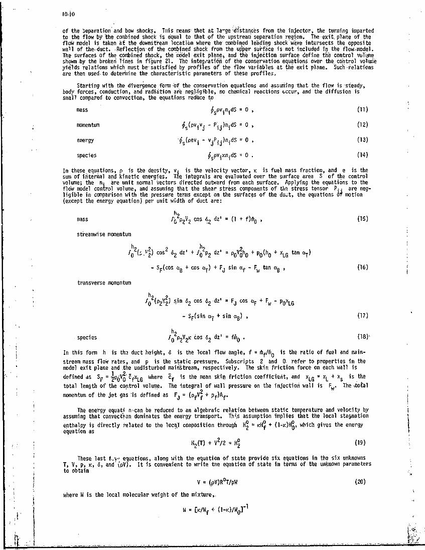
O-io0

of the eparation and bow shocks. This means- that at la-ge distahnes from the injector, the turning impartedto the flow by the combined shock is equal to that of the upstream separation region. The -exit. plane of theflow model is taken at the downstream locatibn where the combined leading shock wave intersects the oppositewall of the-duct. Reflection-of the combined shock from the upper surface is not included in the flow-model.The surfaces of the combinid shock, the m'del exit plane, and the injeftion surface define thb control volumeshown by the broke6i lines in figure 21. The integ,-ation of the conservation equations over the control voluieyi6lds relations which must be satisfied by profiles of the flow variables at the exit plane. Such relationsare then usedto deterfiine the characteristic parameters of these profiles.

Starting with the divergence form of the conservation equations and assuming 'that the flow is 'steady,body forces, conduction, and radiation are negligible, no chemical reactions Gccur, and the diffusion issmall compared to convection, the equations reduce to

mass -spvinidS = 0 , (11)

momentum s(Pviv - P.i )nidS = 0 , (12)

energy -s(pev i - vjP ij)nidS = 0 , (13)

species $spvilnidS 0 . (14)

In these equations, p is the density, v. is the velocity vector, K is fuel mass fraction, and e is thesum of internal and kinetic energies. Tie integrals are evaluated over the surface area S of the controlvolume; the n. are unit normal Vectors directed outward from each surface. Applying the equations to theflow model conlrol volume, and assuming that the shear stress components of the stress tensor P.. are neg-ligible in comparison with the pressure terms except on the surfaces of the du.;t, the equations 6f motion(except the energy equation) per unit width of duct are:

mass 1P2V 2 cos 42 dz' =( +f)0 (15)

streamwise momentum

h 2t c t 2 6dz h2 002 (_."2) c s2 6 dz' + p 2 dz' = PVh + p0 (h0 + XLG tan aT)

- SF(cos a8 + cos aT) + F3 sin af - Fw tan 1B , (6)

transverse momentum

h 2

S0 (P2V2) Ijn 62 cos 62 -dz' = Fj cos QF + Fw - POXLG

" SF(sin a- + sin a) , (17)

- species f02 2 cos 62 dz' = fo " (18)-

In this form h is th2 duct height, 6 is the local flow angle, f = f/O is the ratio of fuel and main-

stream mass flow rates, and p is the static pressure. Subscripts 2 and 0. refer to properties in themodel exit plane and the undisturbed mainstream, respectively. The skin friction force on each wall is

defined as S= 1 6V0 - where Ef is the mean skin friction coefficient, and xLG xL + is the

total length of the control volume. The integral of wall pressure on the injection wall is Fw . The total

momentum-of the jet gas 'Is defined as F= (pfV2 + pf)Af.

The energy equati n-can be reduced to an algebraic relation between static temperature and velocity byassuming that convection dominates the energy transport. his assumption implies that the local stagnation

enthalpy is directly related to the local composition through H0 = KHf + wi gives theequation as 2 f 0

82H(T) + V2/2 = H (19)

These last f ov equations, along with the equation of state provide six equations in the six unknownsT, V, p, K, 6, and' pV). It is convenient to write the equation of state in terms of the unknown parametersto obtain

V = (pV)R°T/pW (20)

where W is the local molecular weight of the mixture,.

W = [IW f 4- (I-K)IW01'I

I-

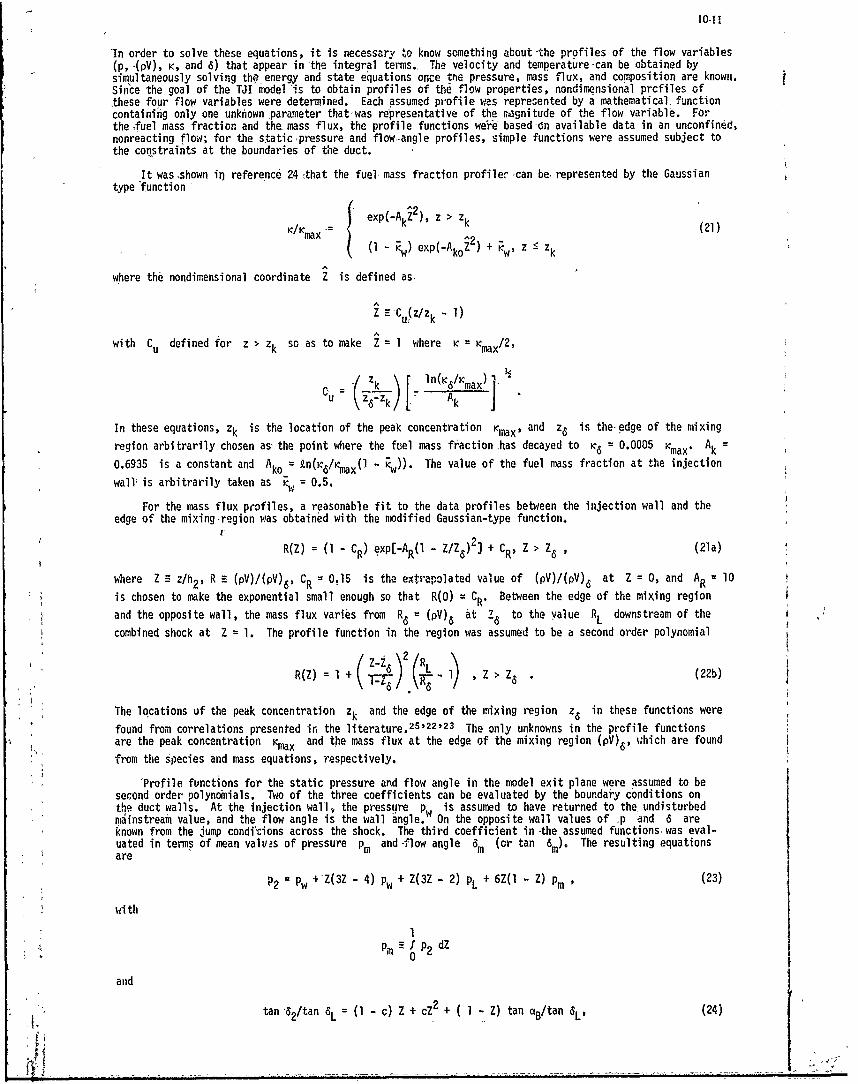
10-11

'In order to solve these equations, it is necessary 'o know something about -the profiles of the flow variables(p, -(pV), K, and 6) that appear in -the integral terms. The velocity and temperature -can be obtained bysimultaneously solving the energy and state equations once tne pressure, mass flux, and composition are known,Since the goal of the TJI model is to obtain profiles of the flow properties, nondimensional prcfiles ofthese four flow variables were determined. Each assumed profile was represented by a mathematical, functioncontaining only one unknown parameter that-was representative of the magnitude of the flow variable. Forthe ,fuel mass fraction and the mass flux, the profile functions we6e based -on available data in an unconfined,nonreacting flow; for the static pressure and flow-angle profiles, simple functions were assumed subject tothe constraints at the boundaries of the duct.

It was shown in reference 24 that the fuel mass fraction profiler -can be represented by the Gaussiantype function

K/ICrx exp(-AkZ2 ), z > zk (21)

(I - w) exp(-AkoZ 2 + wz - zk

where the nondimensional coordinate Z is defined as-

Z -CuZ/Zk - 1)

with Cu defined for z > zk so as to make Z = I where K = Kmaxl2,

(zk) [ n(K6/Kmax)aACu = 1z-lk - k

In these equations, zk is the location of the peak concentration max' and z6 is the-edge of the mixing

region arbitrarily chosen as- the point where the fuel mass fraction has decayed to K6 = 0.0005 Kmax . Ak

0.6935 is a constant and Ako = kn(K6/max(l - w). The value of the fuel mass fraction at the injection

wall is arbitrarily taken as w = 0.5.

For the mass flux profiles, a reasonable fit to the data profiles between the injection wall and theedge of the mixing-region was obtained with the modified Gaussian-type function.

R(Z) (I - CR) exp[-AR(l - Z/Z)2! + CR, Z > Z6 , (21a)

where Z = z/h2 , R (pV)/(pV)6, CR 0.15 is the extrapolated value of (pV)/(pV)6 at Z = 0, and AR = 10

is chosen to make the exponential small enough so that R(O) = CR. Between the edge of the mixing region

and the opposite wall, the mass flux varies from R6 = -(pV)6 at Z, to the value R downstream of the

combined shock at Z 1. The profile function in the region was assumed to be a second order polynomial

R(Z) ; I + Z2) 2 (RL 1) , Z > . (22b)

The locations of the peak concentration zk and the edge of the mixing region z, in these functions were

found from correlations presented in the literature. 25'22'23 The only unknowns in the profile functionsare the peak concentration Kmax and the mass flux at the edge of the mixing region (pV)6 , which are found

from the species and mass equations, respectively.

'Profile functions for the static pressure and flow angle in the model exit plane were assumed to besecond order polynomials. Two of the three coefficients can be evaluated by the boundary conditions onthe duct walls. At the injection wall, the pressure pw is assumed to have returned to the undisturbednmiinstream value, and the flow angle is the wall angle, On the opposite wall values of .p and 6 areknown from the jump condicions across the shock. The third coefficient in -the assumed functionswas eval-uated in terms of mean valu.s of pressure pm and -flow angle 6m (or tan 6m). The resulting equationsare

P2 Pw +Z(3Z - 4) Pw + Z(3Z - 2) PL + 6Z(l - Z) pm (23)

wi th

: 1

Pm- dZ

and

tan' 2/tan 6L = (1- c) Z + cZ2 + (1- Z) tan OB/tan SL' (24)

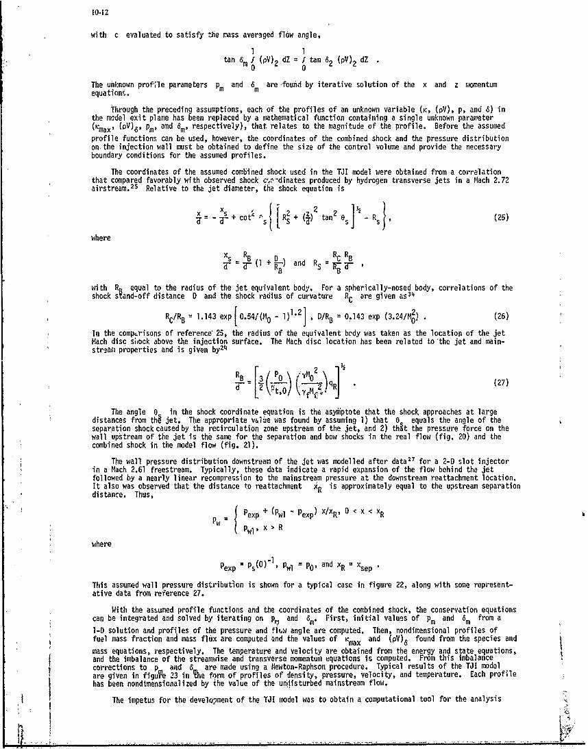
10-12

with c evaluated to satisfy the mass averaged flow angle,

1 1tan 6m f (pV) 2 dZ = f tan 2 (PV)2 dZ

The unknown prof-le parameters pm and 6 are found by iterative solution of the x and z momentumequatinns.

Through the preceding assumptions, each of the profiles of an unknown variable (K, (pV), p, and 6) inthe model exit plane has been replaced by a mathematical function containing a single unknown parameter(Icmax' (PV)tS pm' and Sm' respectively), that relates to the magnitude of the profile. Before the assumedprofile functions can be used, however, the coordinates of the combined shock and the pressure distributionon the injection wall must be obtained to define the size of the control volume and provide the necessaryboundary conditions for the assumed profiles.

The coordinates of the assumed combined shock used in the TJI model were obtained from a correlationthat compared favorably with observed shock c'..-dinates produced by hydrogen transverse jets in a Mach 2.72airstream.25 Relative to the jet diameter, the shock equation is

+ cotr + (-- F- + c l R, .) tan2 es] - Rs}, (25)

where

Xs RB D) and RC RB+ 8(1 S R 7TF ,B B

with RR equal to the radius of the jet equivalent body. For a spherically-nosed body, correlations of the

shock s and-off distance D and the shock radius of curvature RC are given as34

Rc/RB= 1.143 exp 0.54/(M0 - 1)1.2] 1, D/R = 0.143 exp (3.24/M2) . (26)

In the comparisons of reference7 25, the radius of the equivalent body was taken as the location of the jetMach disc si~ock above the injection surface. The Mach disc location has been related to the jet and main-streiam properties and is given by24

R8 3(o) 2- q (27)

The angle 0 in the shock coordinate equation is the asyiiptote that the shock approaches at largedistances from thi jet. The appropriate v&7he was found by assuming 1) that 0 equals the angle of theseparation shock caused by the recirculation zone upstream of the jet, and 2) that the pressure force on thewall upstream of the jet is the same for the separation and bow shocks in the real flow (fig. 20) and thecombined shock in the model flow (fig. 21).

The wall pressure distribution downstream of the jet was modelled after data 27 for a 2-D slot injectorin a Mach 2.61 freestream. Typically, these data indicate a rapid expansion of the flow behind the jetfollowed by a nearly linear recompression to the mainstream pressure at the downstream reattachment location.It also was observed that the distance to reattachment xR is approximately equal to the upstream separationdistance. Thus,

= Pexp + (Pwl Pexp ) x/xR'O < x < xR

Pwl' x > R

where

Pexp Ps(0 ) I Pwl = po' and xR = Xsep

This assumed wall pressure distribution is shown for a typical case in figure 22, along with some represent-ative data from reference 27.

With the assumed profile functions and the coordinates of the combined shock, the conservation equationscan be integrated and solved by iterating on p, and Sm' First, initial values of Pm and 6m from a

1-D solution and profiles of the pressure and fhiw angle are computed. Then, nondimensional profiles offuel mass fraction and mass flux are computed and the values of Kmax and (pV), found from the species and

mass equations, respectively. The temperature and velocity are obtained from the energy and state equations,and the imbalance of the streamwise and transverse momentum equations is computed. From this imbalancecorrections to p ond 6 are made using a Newton-Raphson procedure. Typical results of the TJI modelare given in figure 23 in The form of profiles of density, pressure, velocity, and temperature. Each profilehas been nondimensionalized by ihe value of the unisturbed mainstream flow.

The impetus for the develo2ment of the TJI model was to obtain a computational tool for the analysis

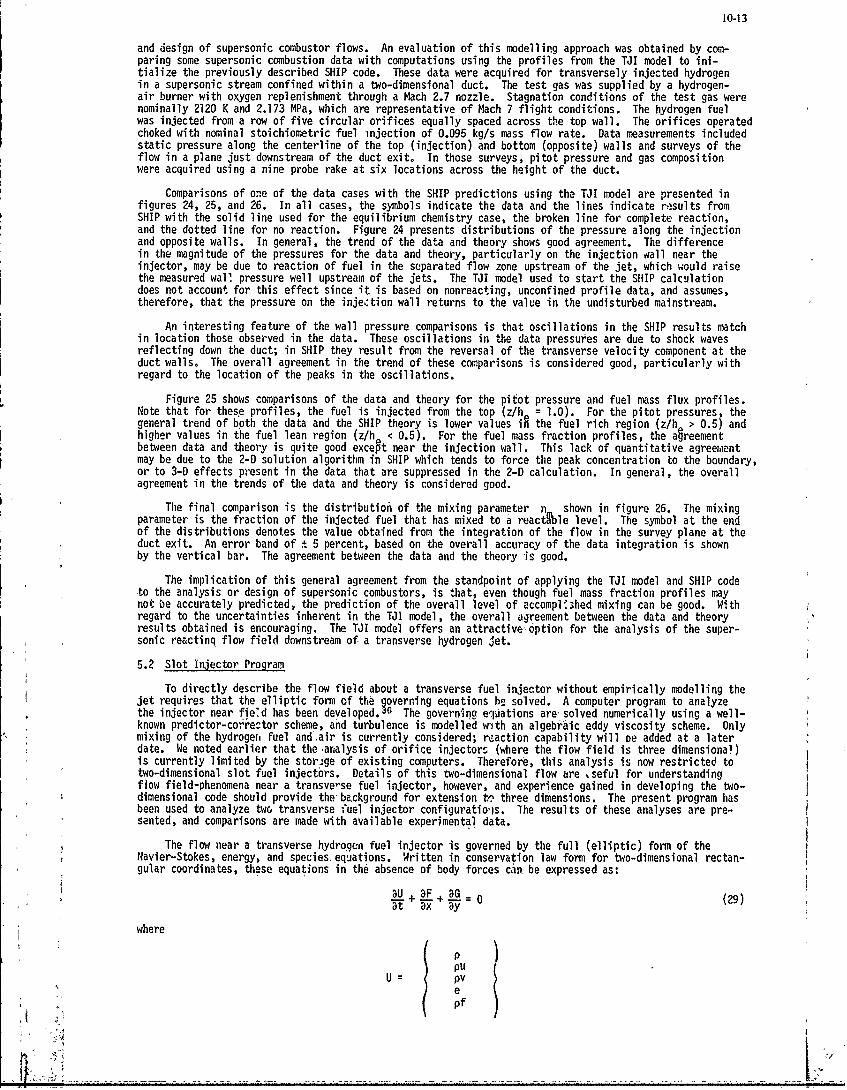
10-13

and design of supersonic combustor flows. An evaluation of this modelling approach was obtained by com-paring some supersonic combustion data with computations using the profiles from the TJI model to ini-tialize the previously described SHIP code. These data were acquired for transversely injected hydrogenin a supersonic stream confined within a two-dimensional duct. The test gas was supplied by a hydrogen-air burner with oxygen replenishment through a Mach 2.7 nozzle. Stagnation conditions of the test gas werenominally 2120 K and 2.173 MPa, which are representative of Mach 7 flight conditions. The hydrogen fuelwas injected from a row of five circular orifices equally spaced across the top wall. The orifices operatedchoked with nominal stoichiometric fuel injection of 0.095 kg/s mass flow rate. Data measurements includedstatic pressure along the centerline of the top (injection) and bottom (opposite) walls and surveys of theflow in a plane just downstream of the duct exit. In those surveys, pitot pressure and gas compositionwere acquired using a nine probe rake at six locations across the height of the duct.

Comparisons of one of the data cases with the SHIP predictions using the TJI model are presented infigures 24, 25, and 26. In all cases, the symbols indicate the data and the lines indicate results fromSHIP with the solid line used for the equilibrium chemistry case, the broken line for complete reaction,and the dotted line for no reaction. Figure 24 presents distributions of the pressure along the injectionand opposite walls. In general, the trend of the data and theory shows good agreement. The differencein the magnitude of the pressures for the data and theory, particularly on the injection qall near theinjector, may be due to reaction of fuel in the separated flow zone upstream of the jet, which would raisethe measured wall pressure well upstream of the jets. The TJI model used to start the SHIP calculationdoes not account for this effect since it is based on nonreacting, unconfined profile data, and assumes,therefore, that the pressure on the inje.:tion wall returns to the value in the undisturbed mainstream.

An interesting feature of the wall pressure comparisons is that oscillations in the SHIP results matchin location those observed in the data. These oscillations in the data pressures are due to shock wavesreflecting down the duct; in SHIP they result from the reversal of the transverse velocity component at theduct walls. The overall agreement in the trend of these comparisons is considered good, particularly withregard to the location of the peaks in the oscillations.

Figure 25 shows comparisons of the data and theory for the pitot pressure and fuel mass flux profiles.Note that for these profiles, the fuel is injected from the top (z/h = 1.0). For the pitot pressures, thegeneral trend of both the data and the SHIP theory is lower values iR the fuel rich region (z/h > 0.5) andhigher values in the fuel lean region (z/h < 0.5). For the fuel mass fraction profiles, the a6reementbetween data and theory is quite good except near the injection wall. This lack of quantitative agreerentmay be due to the 2-D solution algorithm in SHIP which tends to force the peak concentration to the boundary,or to 3-D effects present in the data that are suppressed in the 2-D calculation. In general, the overallagreement in the trends of the data and theory is considered good.

The final comparison is the distribution of the mixing parameter n shown in figure 26. The mixingparameter is the fraction of the injected fuel that has mixed to a reacthle level. The symbol at the endof the distributions denotes the value obtained from the integration of the flow in the survey plane at theduct exit. An error band of :t 5 percent, based on the overall accuracy of the data integration is shownby the vertical bar. The agreement between the data and the theory is good.

The implication of this general agreement from the standpoint of applying the TJI model and SHIP codeto the analysis or design of supersonic combustors, is that, even though fuel mass fraction profiles maynot be accurately predicted, the prediction of the overall level of accomp shed mixing can be good. Withregard to the uncertainties inherent in the TJ1 model, the overall agreement between the data and theoryresults obtained is encouraging. The TJI model offers an attractive-option for the analysis of the super-sonic reactinq flow field downstream of a transverse hydrogen Jet.

5.2 Slot Injector Program

To directly describe the flow field about a transverse fuel injector without empirically modelling thejet requires that the elliptic form of the overning equations be solved. A computer program to analyzethe injector near fie'd has been developed. The governing eq'lations are solved numerically using a well-known predictor-cori'ector scheme, and turbulence is modelled with an algebraic eddy viscosity scheme. Onlymixing of the hydrogen fuel and'air is currently considered; reaction capability will De added at a laterdate. We noted earlier that theanalysis of orifice injectors (where the flow field is three dimensional)is currently limited by the storige of existing computers. Therefore, this analysis is now restricted totwo-dimensional slot fuel injectors. Details of this two-dimensional flow are ,seful for understandingflow field-phenomena near a transve-se fuel injector, however, and experience gained in developing the two-dimensional code should provide the background for extension to three dimensions. The present program hasbeen used to analyze twco transverse fuel injector configuratio,is. The results of these analyses are pre..sented, and comparisons are made with available experimental data.

The flow near a transverse hydrogen fuel injector is governed by the full (elliptic) form of theNavier-Stokes, energy, and species, equations. Written in conservation law form for two-dimensional rectan-gular coordinates, these equations in the absence of body forces can. be expressed as:

a + L+ -= 0 (29)at ax ay

wherebP

pu

U = pve~pf

10-14

Pu

Z + /rx

F= puv + Txy

(e + ox) u + tyxv + qx

pu- fax

PvPuv + 1y

G =pv 2 + Gy

(e + oy) v + Txyu + qyPvf - f

By)and

ax avy au

xy yx ay ax)ry = p - + 2y 2 v

ax - 2iy

2

Pr

Desqx = T -X _

De sqy = -w'B--

By

r =pr (Le =1)

es = cT

11 1lamlnar + "turbulentThe specific heat at constant volume c is a function of the local temperature and species concentrations.

The pressurc is calculated from the equation of state for an ideal gas

p = pROT/W

wh.re the molecular weight W is a function of the local species concentrations. The laminar viscosity iscalculated from Sutherland's law

1.458 x 10-6 T3 kg/-sllaminar - (T + 110.33) /- s

The turbulent viscosity is calculated from an-algebraic eddy-viscosity turbulence model.3

For computational efficiency and accurate resolution of the flow field, the physical coordinate gridmust be fine near the strut walls and the injector where flow-field gradients are large and viscous effectsare important, and the grid must be coarse %,iere flow-field gradients are small and viscous effects lessimportant. Therefore, transformation of thd independent variables with a nonuniform computational gridto a rectangular computational domain with a uniform grid is indicated. Equation (29) is- transfored fromthe physical domain (x, y, t) to the computational domain (X, Y, t) using the independent variable trans-formation of Holst 37 as modified by-Rudy. 38 Equation (29) becomes

au + df F + 1 d 3GT t T 'x - + y 13T- - _ -57 ( 3 0 )

at ~ Y -X Y ~B 031T

All .erivatives in the F and G vectors transform in similar fashion. Their final fortis are:

- dfau I 3V dfaux ( -" y YB dy1 Y 21 dF aX

O-15

-a Txy T- W -YBAY1 3Y 5

0P \~p- X +yyA YBdA y BdY1-

= es dfq x K3T TX

, dg

The f Uctioiihs and g' compr'es' t06 grid iiai Walls-and fuel, injectors.

The tiie-split finite difference technique of MacC6rniack5 9 is 0sed to integrate the governing equationsuntil a steady-state solution is reached. 0 fa solution to equation (3U)'is known at sce time t = nAt,Sthe solution at the next time step, t' = in,+, l)At dai be calculated froni

vn+lt = L (At) U.9 . (31)1,0 1,9I,

for each node point (i,j) in a finite difference grid network within the boundaries of the computationaldomain. The finite difference operator L is split info two oheoimiensional difference operators L (At)and L(At) Each split operator-consists of a predictor and corrector ihtegration step; Lx is definedby , J...

un+l: x(ax n

where- U At

i =l~ ~--F i " l,j (32)

Au n F~ - -~ [\,un+l, I U n +,Un+T ntx n+ (3• "~ j S i+l,j w Tx ] "(3

L is defined byK yUn +l L, (At U

where

n Ati,j i,j AY i,j " Gy

n. +U + _ ty(j f '___ Ii~ ~ ~Gj~ 2n1 li+AY 4 (35)

i~j 2 ipj Aj Y ijl"i IYA YB y

'First derivatives in the F and G terms are differenced as follows. In the, L operator all partialderivatives with respect to x i ontained in F are fol.ard-differehced in the pedictor and backward'differenced in the corrector. All derivatives with respect to y 'are central differenced in both-the pre-dictor and corrector. In the L operator, all partial.derivatives-wif respect to y are forwarddifferenced in the predictor andbackWard differenced in 'c'he corrector, and-all derivatives with respectto x, are central differenced. The one-dimensibnal operators are combined-tb form a two-dimensionaloperat6r through the symetric operator sequiice3s

((At) At) (At)- A t (36)

One pass through equation, (36) advances the finite difference form of erquation (30) through one time step,At.

Boundary conditions of the reflection type were used along walls or planes 6of symmetry.9 For a wall

along the lower boundary of' the physical domain, no sl ip~conditians (u -0, i = 0); require

ui,= l ui, 2 (37)

vi,= vi, °(38)1

-

The-wall is-assumed adiabatic so that the normal derivative of temperature must vanish. This gives

Ti - (39)

10-16

The normal derivative of thehydrogenmass fraction is also required to vanish consistent with the no fluxcondition at a wall giving

fil = f i,2 (40)

The pressure and density along the boundary nodes are set equal to the values at adjacent nodes.

Pi,l = Pi,2 (41)

Pi,l = Pi,2 (42)

These boundary conditions are applied during both the predictor and corrector steps while integrating thecontinuity, momentum, energy, and species equation5. For a wall along the upper physical buUndary, equations(37) through (42) again specify (with an appropriate change of the j node index) the required boundaryconditions. For a symmetry plane along the upper boundary, equations (37) and (38) become

Ui,nny = Ui,nny-l (43)

vi,nny = -vi,nny.l (44)

but equations (39) through (42) remain unchanged. Boundary conditions along the inflow plane are specifiedby holding all dependent variables fixed at their initial values. Along the outflow station all dependentvariables are calculated by linear extrapolation from upstream values. At a hydrogen fuel injector, boundaryconditions are specified by fixing all dependent variables at their initial values consistent with the re-quired physical behavior of the jet. Initial conditions are normally specified before beginning a calculationby assuming that free-stream conditions exist at all nodes for each dependent variable.

Artificial viscosity must be added near the bow shock and reattachment shock to smooth pressure andtemperature oscillations that develop in those regions. The fourth order numerical damping technique ofMacCormack 39 is effective in smoothing these oscillations with moderate injector to free-stream pressureratios. For high pressure ratios, the numerical diffusion cancellation method is employed. Details regard-ing the application of both techniques are given in reference 36.

Calculations have been performed for two test cases that consider sonic transverse injection of hydrogeninto a- :upersonic air cross stream. The first case represents a two-dimensional equivalent of the flowbetween two scramjet engine struts with geometrically opposing hydrogen fuel injectors. Results from thisanalysis give insight into the nature of the flow field near fuel injectors and indicate likely locationsfor ignition of the fuel-air mixture that is present. The second case considers the sonic slot injectionof hydrogen from a flat plate at zero angle of attack in a supersonic cross flow. Experimental wall dataare available for the latter case, and comparisons of the data with the computer program are discussed inthis section.

The configuration of the first case is shown in figure 27. Gaseous hydrogen is injected from two 0.127cm slots at

M 1.1

T = 242 K

p =0.526 MPa

into a 6 cm high by 10 cm long duct having the following inlet air conditions

M =2.7

T = 800 K

p =0.101 MPa

The turbulent Prandtl Number was assumed to be 0.9. The physical domain was spanned by a finite differencegrid with 39 nodes in the streamwise direction and 30 nodes in the transverse direction. Due to symmetryabout the duct centerline, calculations were carried out only in the region between the lower wall and theduct centerline. The grid was compressed normally near the wall and in a streamwise direction about theinjectors with transformation constants (ref. 37) specified as

a=7.8

yX =5,0 cm

The inflow station was placed approximately 1.5 cm upstream of the duct entrance. That placement was neces-sary to prohibiL downstream events from propagating upstream through the subsonic region of the wall boundarylayer to the inflow station where flow conditions were fixed. The outflow station was placed 5 cm downstreamof the injectors where the flow was again predominantly supersonic to minimize the effect of the outflowboundary conditions on the flow field near the injectors.

Overall results from the first case are shown in figures 28 through 32. In each case the region being=displayed lies between the lower duct wall and the duct centerline. The injector is located in the center

7

10-17

(X = 5 cm) of the computational domain. Figure 28 shows a plot of the velocity vector field in the lowerhalf duct. Values of the uniformly spaced vectors are interpolated from nodal values on the ronuniform grid.The expected features of the flow field have been predicted by the analysis. The separated region upstreamof the injector is apparent in the plot as indicated by a reversal of the velocity vectors that form a re-circulation pattern. The separation shock that results from the thickened boundary layer upstream of theseparation region can also be seen through a small upward deflection of the velocity vectors. The separationshock merges into a bow shock that turns the main-stream flow over the injector. The bow shock is quitestrong and can be observed in figure 28 through a large upward deflection of the velocity vectors as theflow is processed by the shock. The downrunning bow shock from the upper injector (actually, in this case,a centerline reflection of the uprunning shock) is indicated by the velocity vectors as they turn downwardfrom the centerline just beyond the point where the shock strikes the centerline. Inspection of the flowfield in figure 28 near the injector shows that the hydrogen jet is turned in a nearly streamwise directionrather quickly by the air cross stream. Blockage of the cross flow by the jet results in another separatedreuion behind the injector which can also be seen in the vector plot. The location of the reattachmentshock following this separated region is not obvious in figure 28, but some indication of the shock is pre-sent in figure 29 where the velocity vectors turn from the wall and reorient in the mainstream direction.Figure 29 shows a magnified vector plot near the hydrogen injector. The region being considered is centeredabout the injector arid has a range of

2.5 cm : x 9 7.5 cm

0 cm : y S 1.5 cm

Velocity vectors are not plotted when their values become less than 5 percent of the maximum vector in thefield. Examination of the recirculation region upstream of the injector reveals the presence of two counter-rotating eddies known to be present in the physical flow.

Figure 30 shows a contour map of the static pressure Field in the duct. Each contour line representsa difference in pressure of 0.02 NPa. The presence of the separation shock, the bow shock, and its reflec-tion can also be seen in this figure through pressure rises across the shocks. (Shocks are captured andsmeared by the present analysis, and therefore, pressure rises across the shocks occur over some finitedistance. This broadening of the shock structure results in a merging of the separation and bow shocks mak-ing visual resolution of the two shocks impossible.) The expansion of the hydrogen jet into the air crossstream can be seen along with the expansion of the hydrogen-air mixture over the injector. There is alsosome indication of a duct entry shock being captured, producing a small pressure rise across the shock.

Figure 31 displays a contour map of the static temperature field in the duct. Each contour line rep-resf 's a change in temperature rf 70 K. Note the temperature rise across the bow shock and the thermalboundary layer along the wall that thickens with movement towards the fuel injector. Significant coolingof the air by the expanP'1g hydrogen jet can also be seen, particularly behind the injector. Some coolingis also experienced in One separated region upstream of the injector due to the limited presence of hydrogen.

Figure 32 provides a contour map for the hydrogen mass fraction distribution in the duct. Contour linesare plotted for hydrogen mass fractions of 0.75, 0.50, 0.25, and 0.01. With a static jet to static free-stream pressure ratio of 5, the penetration of the hydrogen jet into the air cross stream is significant.The one percent hydrogen contour line lies at 1/5 the duct height after proceeding only 2 cm downstream.The recirculating region upstream of the injector convects hydrogen forward of the J~t, and the mixture goesfrom fuel lean to fuel rich as the slot is approached. The separated flow downstream of the slot captureshydrogen producing a very fuel rich region. These characteristics of the flow have been experimentallyobserved in scramjet tests; the upstream region provides a beneficial area for fuel ignition, and the down-stream region (being fuel rich) imposes an ignition problem.

The first test case provides an examination of opposing slot fuel injectors using actual flow fieldconditions encountered in current scramjet engine concepts. The basic features of the flow desiribed abovecompare well qualitatively with experimental observations near a fuel 4rojector. Additionally, graphicalrepresentations of the final results, used to describe this case, provide a quick visualization of the over-all flow field, as-well as interesting details near the fuel injectnrs.

The second test case provides a comparison of the computer program with experimental data. 41 Gaseoushydrogen was injected from a choked 0.02 cm slot on a flat plate at zero angle of attack into a supersonicair cross stream. The slo t was 5.08 cm long and located 25.6 cm from the leading edge of the plate. Theflow field with this slot length was verified in reference 41 to be two dimensional within the region ofinterest. A turbulent boundary layer was produced by tripping the flow 2.54 cm from the plate leading edge.This experiment represented the only case known to the authors, in which species measurements were made todetermine hydrogen concentration away from the slot. The case was by no means ideal for verification of thepresent computer program, however. The jet to free-stream pressure ratio was significantly higher thanratios encountered in scramjet design (a static jet-to-freestream pressure ratioof 43 as compared to pressureratios of 5 to 15 expected in a scramjet), and the slot width was quite narrow. These two conditions combinedto produce extremely large gradients near the slot, complicating a numerical ana'ysis of the problem. Largeflow field gradients also complicate the accurate acquisitior, of data near a fuel injector. In addition,only conditions along the wall upstream of the slot were measured. No survey. were available away from theplate.

The conditions of the hydrogen at the slot exit were

= 1.0

T = 243 K

p = 7.28 4Pa

10-18

The conditiOhs of the air just upstream of theleading edge of lhe flat platewe-e

M-= 2;5

V= 130K

p-= 0.169MPa

Two approaches were considered to define the computational domain for this case. -In both approaches the do-main was chosen to be 6-cm high and10 cm 'long with the injector centered along- the lowef'boundary. The over-all plate lengthmade it impracticable to begin the calculation at the leadingedge. Therefore, for the first-approach, -initial -conditions were specifid, by assuming thepreseice of a turbulent boundary layer on theplate:beginningat the leading edgewith the boundary layer thickness defined by

42

+ (o ,= ) -II

0~ ~~ U.I Q( ~6 = 0.37 x \ PT

} The streamwise velocity in the boundary layer was defined using the one-seventh power law distribution42

1/7

For the second approach, the calculation was initialized assuminguniform free-stream conditions throughthecomputational domain (as in the first case). Ther6e was little difference in the final §teady-state-results-of the two approaches.. The similarity was likely due to the fact that the subsonic portion of the~boundarylayer well upstream of the slot was quite thin when compared with the thickened boundary layei near the slot,pand theore, the conditions near the injector were relatively insensitive to c6nditio6s near the Plate well~upstream.

The- turbuieit Pandtl number in this case was assumed to be,0.7. The physical domain was spanned by a

grid with 61 nodes in the streamwise direction and 30 nodes in the transverse directioi. Free-stream condi-tions were assumed to exist along the upper boundary. The grid was again compressed ti'ansversely near 'theplate and in a streamWise direction about the injector with %he following transformation constants (ref. 37):

ll,.28

= 1.002

xi =5.0 cm

Comparisons of experimentally measured valupt .f wall,pressure and hydrogen mass fraction upstream ofthe! slot with calculated values from the present +analysis are ade infigures 33 and 34, respectively. Thecalculated~wall pressure ,(fig. 33), ahs the same basic shape as the experimental data but the calculated pres-sure rise begins at about 120 slot widths upstream of the injector as compared to the experimental pressurerise that~begins at about 175 slot widths upstream of the injector. Calculated and experimental values ofwall pressure aye similar through the last100 slot widths upstream of the injector, and there is reasonablygood agreement for wall plateau pressures. Figure 34 presents a comparison of computed and measured valuesof hydrogen'mass fraction along the plate upstream of the injector- The calculatioi underestimates the amountof hydrogen present initialli Closer to the slot (100 'lot widths or less) the calculation of the hydrogenmass fracton agrees fairly -

' 1l When compared wjith the experiment.

-Differences between the calculation dnd experiment are attributable to two basic problems, the turbulencemodel and the -numerics. Underprediction of the point of separation initiating a- recirculation region upstreamof a disturbance, with the resulting underprediction of initiation of- the-ywall pressure rise, -is typical ofearlier observations by other researchers. In those cases, as well as in the present analysis, the point ofseparation is a strong function of the turbulence field in the flow. Other turbulence models have been ap-plied to th6piesent problem, and resulted'in a significant variation in the separation point and the size ofthe recirculation region. The Present turbulence mdel, 3 however, gives the most consistent overall' resultswhencoma'red with the experimental data' In such a complex turbulent mixing. flow, a simple algebraic eddyviscosity. turbulencemodel.is obviously inadequate. -Non-equilibrium effects are quite important in the sep-4arated region near the ijector,-and the turbulence field, in this region is certain to be -highly anisotropic.Neithr-effecthas been accounted for in the models that have been used'.

-Oscillations present in the results of figures 33-and 34 between 30 and '80 slot widths upstream of theinjector are likely t6 be numerical in-origin. A very strong bow shock resulting from the highly underexpand~dhydrogen-injector was captured in this region. Pressure Oscillationh leadingand tiailing a significant staticpressure increase-when passing through a shock are typical occurrences with the present technique. Oscilla-tions are also present very-near the slot (0o1 cm), but the oscillations wer&- small compared to the overall-prsur is 0.7to73+~ ). Severe gradients are~experienced near the injector that require an extremelyfine grid to adequately resolve. Even though the present grid is highly compressed near the bow shock and

injector, truncation error is likely to be significant inthis region.

To more accurately predict the complex flow regime near a fuel injector, the following changes to theprogram and its appl'ication are indicated-, First, the turbulence model must be improved to account for theanisotropic nature of the turbulence field. Solution of the Reynolds stress equationsseems premature-atthis point. However, application of the algebraic Reynolds stress model of Rodi 4 3 is promising since itwould-partially account for the anisotropy. Second, a finer discretization-obtained by employing a larger

- - number of nodes near fuel injectors would better resolve high gradients in this region. Computer core limita-tions restrict the number of nodes that can be considered,however. Finally, shock -capturing, with-attendantnumerical smoothing, smears the separation and bow shock over A relatively large-distance introducing error

10-19

downstream of the shocks. Fitting those shocks would-produce a much better spatial resolution of the flowvariables downstream of the discontinuities.

The two-dimensional elliptic program represents a first attempt to model a transverse injector with apurely numerical approach. Experience gained during the development of the program should be helpful whenthe work is extended to three dimensions. That extension is currently limited by computer resources andrequired processing time. The two7dimensional program does allow study of the basic flow field phenomenaaround a transverse fuel injector and this new capability should provide guidance in the ongoing scramjetdesign effort.

The transverse jet interaction model and the slot injectorprogram provide two -options for initializinga parabolic flow calculation downstream of the elliptic region surrounding fuel injectors. The TJI schememodels the fuel injector and is limited to inviscid flow. The program -s computationally efficient, however,allowing parametric analyses to be carried out at modest cost. The slot injector program directly solvesthe governing equations describing viscous flow about transverse fuel injectors. Additionally, the programcan consider other problems such as rearward facing steps upstream of the fuel injectors. Relaxing thegoverning equations to steady state is time consuming, however, making the procedure rather expensive forparametric studies. Therefore, extension of both the TJI model and the slot injector program to three dimen-sions is planned. Each program will be used to calculate initial conditions for the three-dimensional para-bolic or partihlly elliptic program downstream of the fuel injectors. The coupling of these programs willprovide an overall combustor analysis tool to aid in the design of the Langley scramjet engine.

6.0 CONCLUSIONS

A system of computer programs has been developed at the NASA Langley Research Center to model the com-bustor of a scramjet engine. The engine flow field can be divided into several physical flow domains, eachof which can be described by appropriate forms of the Natier-Stokes and companion species equations. Aprogram based-on those governing equations has been developed for each region, and the programs are beingcombined to form an overall computational capability for scramjet combustor design. Some programs in thesystem have progressed to the design stage, and they are now being applied to actual combustor configurations.The remaining programs continue to be developed, but they already provide basic research tools for limitedengine applications.

The parabolic flow computer programs are based on proven solution algorithms, and have been improved toinclude an appropriate turbulence model and multiequation finite rate chemistry models considered adequatefor modelling supersonic combustor flow fields. Recent comparisons of the programs with experimental datahave been quite encouraging. The partially elliptic computer program has proved effective for describingsubsonic flow without separation in the combustor, but development is still continuing to provide a satis-factory convergence criteria for the computed pressure field. Results comparing parabolic and partiallyelliptic calculations in subsonic flow indicate differences sufficient enough to warrant continued work inthis area. Elliptic programs, used to model the flow field near transverse fuel injectors are the mostrecent addition to the analysis system. Current two-dimensional analyses compare favorably with experimentaldata, but further work is needed, particularly to model the complex turbulence fields and chemical reactions.Extension of the elliptic flow program to three dimensions is limited by storage problems to all but thelargest current or future vector computers until significant advancements occur in integration algoritoms.

Further work is planned in turbulence and reaction modelling that will impact all of the combustoranalysis programs. The highly anisotropic turbulence fields that must exist in some regions of the combus-tor must be considered in greater detail, Current interest exists for solution of the Reynolds stressequations to model the turbulence. Application of the algebraic Reynolds stress model of Rodi may offer anear term solution to that problem. Chemistry models will be extended to include the details of reactionand ignition in hydrogen-air reactions. Finally, the importance ot coupling between chemical reaction andturbulence must also be considered in greater detail. The impact of that coupling on combustor modellingis not well underst6od at present. The current capabilities to model the scramjet combustor flow field do,however, represent an important step forward in engine design, and should provide guidance in the ongoingscramjet development effort at the NASA Langley Research Center.

REFERENCES

1. Jones, R. A., and Huber, P. W., "Toward Scramjet Aircraft," Astronautics and Aeronautics , vol. 16,Feb. 1978, pp 38-48.

2. Hearth, D. P., and Preyss, A. E., "Hypersonic Technology - Approach to an Expanded Program," Astro-nautics and Aeronautics, vol. 14, Dec. 1976, pp 20-3}.

3. Baldwin, B. S., and Lomax, H., "Thin Layer Approximation and Algebraic Model for Separated TurbulentFlows," AIAA Paper No. 78-257, Jan. 1978.

4. Launder, B. E., and Spalding, D. B., "The Numerical Computation of Turbulent Flows," Computer Methodsin Applied Mechanics and Engineering, vol. 3, 1974, pp 269-289.

5. Bahi, G. S., "Calculations on the Autoignition of Mixtures of Hydrogen and-Air," NASA CR-112067,Apr. 1972.

6. Evans, J. Z., and Schexnayder, C. J., "Critical InFluence of Finite Rate Chemistry and Unmixedness onIgnition and Combustion of Supersonic H2-Air Streams," AIAA Paper No. 79-0355, Jan. 1979..

7. Spalding, D. B., Launder, B. E., Morse, A. P., -and Maples, G., "Combustion of Hydrogen-Air Jets inLocal Chemical Equilibrium (A Guide to the CHARNAL Computer Program)." NASA CR-2407, 1974.

8. Elghobashi, S., and Spalding, D. B., "Equilibrium Chemical Reaction of Supersonic Hydrogen-Air Jets(The ALMA Computer 'Program)," NASA CR-27z- 1977.

10-20

9. Patankar, S. V., and Spalding, D. B., "Heat and Mass Transfer in Boundary Layers," Int. Textbook Co., Ltd.(London), Second ed. Int., 1970.

10. Dash, S., Weilerstein, G., and Vaglio-Laurin, R., "Compressibility-Effects in Free Turbulent ShearFlows," Air Force Office of Scientific Research, TR-75-1436, Aug. 1975.

11. Speigler, E., Wolfshtein, M., and anheimer-Timnzt, Y., "A Model of Unmixedness for Turbulent ReactingFlows," Acta Astronautica, vol. 3, 1976, pp 265-280.

12. Kent, J. H., and Bilger, R. W., "Measurements in Turbulent Jet Diffusion Flames," TN F-41, Dcpt. Mech.Eng., Univ. Syndey (Australia), Oct. 1972.

13. Salas, Manuel D., "Shock Fitting Method for Complicated Two-Dimensional Supersonic Flows," AIAA J.,vol. 14, no. 5, May,1976, pp 583-588.

14. Markatos, N. C., Spalding, D. B., and Tatchell, D. G., "Combustion of Hydrogen Injected into a Super-sonic Airstream (The SHIP Computer Program)," NASA CR-2802, 1977.

15. Pan, Y. S., Drummond, J. P., and McClinton, C. R., "Comparison of Two Computer Programs by PredictingTurbulent Mixing of Helium in a Ducted Supersonic Airstream," NASA TP-1166, 1978.

16. Pan, Y. S., "Evaluation of the Three-Dimension,l Parabolic Flow Computer Program SHIP," NASA TM-74094,1978.

17. Patankar, S. V., and Spalding, D. B., "A Calculation Procedure for Heat, Mass, and Momentum Transferin Three-Dimensional Parabolic Flows," Int. J. Mfeat and Mass Transfer, vol. 15, 1972, pp 1787-1806.

18. McClinton, C. R., "Evaluation of Scramjet Combustor Performance Using Cold Nonreactive Mixing Tests,"AIAA Paper tlo. 76-47, 1976.

19. Burrows, M. C., and Kurkov, A. P., "Supersonic Combustion of Hydrogen in a Vitiated Air Stream UsingStepped-Wall Injection," AIAA Paper No. 71-721, 1971.

20. Burrows, M. C., and Kurkov, A. P., "An Analytical and Experimental Study of Supersonic Combustion ofHydrogen in a Vitiated Airstream," AIAA Journal, vol. 11, 1973, pp 1217-1218

21, Pan, Y. S. "The Development of a Three-Dimensional Partially Elliptic Flow Computer Program for CombustorResearch," NASA CR-3057, 1978.

22. Pratap, V. S., and Spalding, D. B., "Numerical Computations of the Flow in Curved Ducts," The Aero-nautical Quarterly, vol. 26, 1975, pp 219-228.

23. Hjertager, B. H., and Magnussen, B. F., "Computation of Some Three-Dimensional Laminar IncompressibleInternal Flows," Proc. of 25th Heat Transfer and Fluid Mechanics Institute Meeting, Stanford UniversityPress, 1976, pp 436-451.

24. Rogers, R. C,, "A Model of Transverse Fuel Injection Applied to the Computation of Supersonic CoitustorFlow," AIAA Paper No. 79-359, 1979.

25. Orth, R. C., Schetz, J. AI, and Billig, F. S., "The Interaction and Penetration of Gaseous Jets "nSupersonic Flow," NASA CR-1386, 1969.

26. Werle, M. J., Driftmyer, R. T., and Shaffer-, D. G,, "Two-Dimensional Jet Interaction with a Mach 4Airstream," NOLTR-70-50, 1970.

27. Spaid, F. W., and Zukowski, E. E., "A Study of the Interaction of Gaseous Jets from Transverse Slotswith Supersonic Externa, Flow," AIAA J., vol. 6, no. 2, 1968, pp 205-212.

28. Zakkay, V., Calarese, W.i and Sakell, L., "An Experimental Investigation Between Trans rse Sonic Jetsand a Hypersonic Stream," AIAA J., vol. 9, no. 4, 1971, pp 674-682.

29. Spaid, F. W., Zukowski, E. E., and Rosen, R., "A Study of Secondary Injection of Gases into SupersonicFlow," Jet Propulsion Lab. Tech. Rpt. 32-834, 1966.

30. Werle, M. J., "A Critical Review of Analytical Methods for Estimating Control Forces Produced by SecondaryInjectioni" NOLIR 68-5, 1968.

31. Schetz, J. A., Hawkins, P. F., and Lehman, H., "Structure of Highly Underexpanded Transverse Jets in aSupersonic Stream," AIAA J., vol. 5, no. 5i pp 882-884.

32. Cohen, L. S., Coulter, L. J., and Egan, W. J., Jr., "Penetration and Mixing of Multiple Gas Jets Sub-jected to a Cross Flow," AIAA J., vol. 9, no. 4, 1971, pp 718-724.

33. Rogers, R. C., "Mixing of Hydrogen Injected from Multiple Injectors Normal to a Supersonic Airstream,"NASA TM D-6476, 1971.

34. Billig, F. S., "Shock-Wave Shapes Around Spherical an Cylindrical Nosed Bodies," J. of Spacecraft,vol. 4, no. 6, 1967, pji 822-823.

35. Rogers, R. C., "Influence of iuel Temperature on Supersonic Mixing and Combustion of il1drogen," AIAAPaper No. 77-17, 1977.

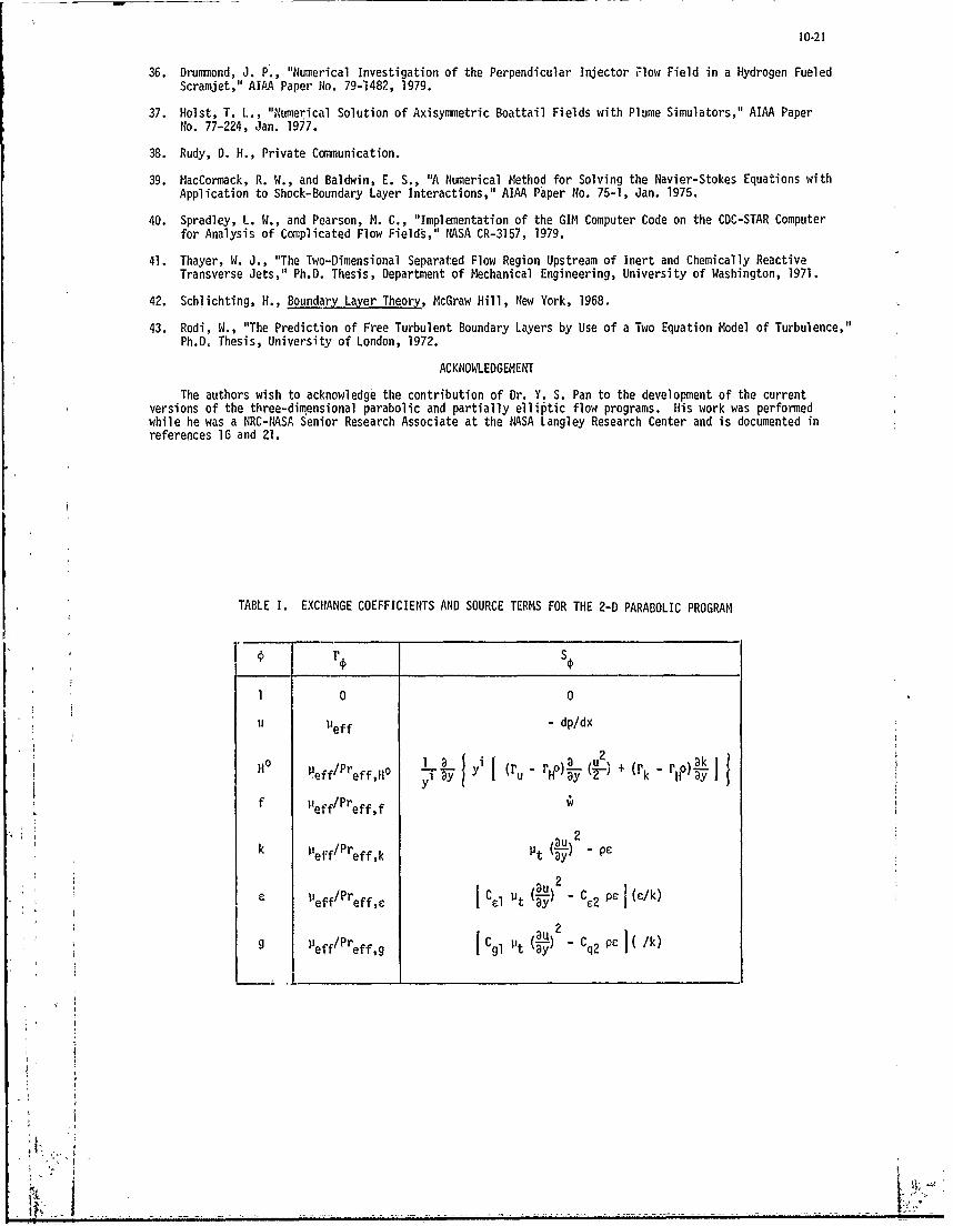
10-21

36. Drummond, J. P., "Numerical Investigation of the Perpendicular Injector -low Field in a Hydrogen FueledScramjet," AIMA Paper No. 79-1482, 1979.

37. Holst, T. L., "Numerical Solution of Axisymmetric Boattail Fields with Plume Simulators," AIAA PaperNo. 77-224, Jan. 1977.

38. Rudy, D. H., Private Communication.

39. NacCormack, R. W., and Baldwin, E. S., "A Numerical Method for Solving the Navier-Stokes Equations withApplication to Shock-Boundary Layer Interactions," AIAA Paper No. 75-1, Jan. 1975.

40. Spradley, L. W., and Pearson, M. C., "Implementation of the GIM Computer Code on the CDC-STAR Computerfor Analysis of Complicated Flow Fields," NASA CR-3157, 1979.

41. Thayer, W. J., "The Two-Dimensional Separated Flow Region Upstream of Inert and Chemically ReactiveTransverse Jets," Ph.D. Thesis, Department of Mechanical Engineering, University of Washington, 1971.

42. Schlichting, H., Boundary Layer Theory, McGraw Hill, New York, 1968.

43. Rodi, W., "The Prediction of Free Turbulent Boundary Layers by Use of a Two Equation Model of Turbulence,"Ph.D. Thesis, University of London, 1972.

ACKNOWLEDGEMENT

The authors wish to acknowledge the contribution of Dr. Y. S. Pan to the development of the currentversions of the three-dimensional parabolic and partially elliptic flow programs. His work was performedwhile he was a NRC-NASA Senior Research Associate at the NASA Langley Research Center and is documented inreferences 16 and 21.

TABLE I. EXCHANGE COEFFICIENTS AND SOURCE TERMS FOR THE 2-D PARABOLIC PROGRAM

r S

1 0 0

u Ueff - dp/dx

eff/Preff, 1

ljffPry' (ru -'ii)7 L-( + (rk - 140) Lk

2

I 3u 2

9 P ef/Pref ~ I PC5 1 ( 3y - ci(/k)

eff/Preff,g Cgl I1t 3y - C P 1(/k)

I

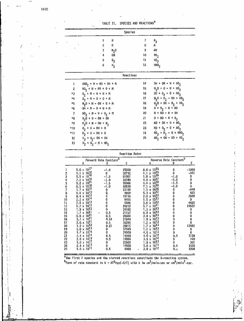
10-22

TABLE II. SPECIES AND REACTIONS a

Species

I H 7 N22 0 8 N

3 H20 9 NO

4 OH 10 NO25 02 i1 HO26 H2 '12 HNO 2

Reactions

1 HNO 2 + M NO + OH +M 14 OH + OH H + HO22 N02 + M NO + 0 + M 15 H90 +0 H + HO 2*3 H2 + M H + H + M 16 H + 02 0 + HO2*4 02 + M O+ 0O+M 17 H20 + 02 -0H + HO2*5 H20+ M OH + H + M 18 H0 + OH+ H2 + HO2

*6 OH + M- 0 + H + M 19 0 + N2 -4 N + NO

7 HO2 +M H + 02 +M 20 H + NO N + OH*8 820+ 0 OH + OH 21 0-+ NO- N +0 2

*9 H2 0+ H -OH + H2 22 NO + OH- H + N02

*10 02 + H OH + 0 23 NO, + 02 0 + N02

*11 H2 + 0 OH + H 24 NO2 +l 2 H+HNO2

12 H2 + 024 OH + OH 25 NO2 + OH -NO + H0213 H2 + 0 - HO2

Reaction Rates

Forward Rate Constantb Reverse Rate ConstantbA B C A B C

1 5.0,x 017 -1.0 25000 8.0,x 1015 0 -10002 1.1 ; 1016 0 32712 1.1 x 1015 0 -9413 5.5 x 018 -1.0 51987 1.8 x 1018 -1.0 04, 7.2 x 1018 -1.0 59340 4.0 x 1017 -1.0 05 5.2 x 1021 - 59386 4.4 x 1020 -1.5 06 8.5 x 1018 -1.0 50830 7.1 x 1018 -1.0 07 1.7 x 1016 0 23100 1.1 x 1016 0 -4408 5.8 x 1013, Q 9059 5.3 x 1012 0 5039 8.4 x 1013 0 10116 2.0 x 1013 0 2600

10 2.2 x 1014 0 8455 ! x 1013 0 011 7.5 x 1013 0 5586 3.0 X 101 3 0 442912 1.7 x 1013 0 24232 5 x7 x 01 0 1492213 1.9 x 1013 0 24100 1.3 x 1013 0 014 1.7 x 1011 0.5 211B7 6.0 x 1013 0 015 :5.8 x 1011 O.5 28686 3.0 x lc1 3 0 016 3,7 x 1011 0.64 27840 1.0 x 1013 0 017 2.0,x 1011 0.5 36296 1.2 x 1013 0 018 1.2 , 1012 0.21 39815 1.7 x 1013 0 1258219 5.0 x 1013 0 37940 1.1 x 013 0 020 1:.7 x 1014 0 24500 4.5 x 1013 0 021 2.4 x 1011 0.5 19200 1.0 x 1012 0.5 312022 2.0 x 1011' 0.5 15500 3.5 x 1014 0 74023 1.0 x 1012 0 22800 1.0 x 1013 0 30224 2.4 x 1013 0 14500 5.0 x 1011 0.5 150025 .0 x 1011 0.5 6000 3.0 × 1012 0.3 1200

aThe first 7 species and the starred reactions constitute the 8-reaction system.bForm of rate constait is k ATBexp(-C/T) wmth k in cm3/mole-sec or cm /mole -sec.

.. .. _ _... _ _I

10-23

TABLE Ill. EXCHANGE COEFFICIENTS AND SOURCE TERMS FOR VARIABLE @

r S

1 0 0

Ueff " 1 + . i-T-" (Lu - 2a-) + [ peff L"ef ax, 3 ~3x a~yJ aye afxJ

!e -f+L (L . eff ___ _

efY Dy j 3 ay 'x' a x a efyJ

w 1eff -z

Ho Ieff [neff (Pr i?-) (u +V 2 + 4Pr eff,Ho ax Preff,Ho ef f, , x 2 2)

3 '[eff 2P re *L 2 +W2 +Ty r.~ eff3'

L2 ~2 Du__Peff I(~ ax (L) + 2 TU TV

f 11eff 0Preff,f

Preffk 3w @" 'B' "x B

Peff u t 2 2I( + ' " +" +

Peff ~C1 C f2 {Rj 'U + (av3 I +gFreffc

a

S(2w) 2 + au + v 2 c2ay aii ax) C2'

1*

S HOCK Lf ~ R UST

SCHEM ATIC OF

ENGINE CROSS SECTION " NOW,'

Fig. 1. Hypersonic vehicle with airframe-iintdgrated scramiet. Fig. 2. Scramiet engine module.

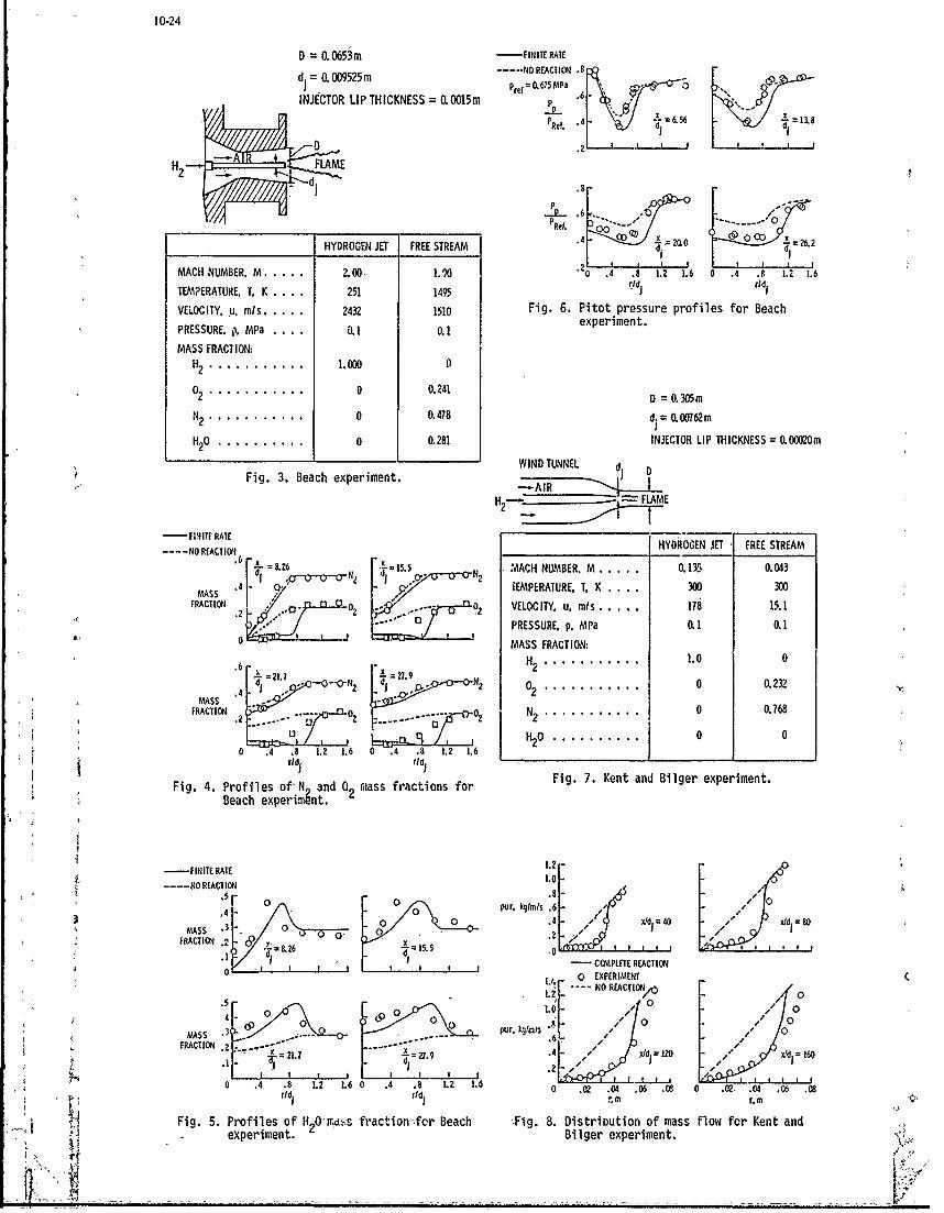
10-24

D = 0. 0653mIT -FINITE RATE

d0. O009525mIT---ORATO .8

INJJECTOR LIP THICKNESS 0. O0015 In .6

PO '4 6.61.8

-FLAME

NIL /0

HYDROGEN JET FREE STREAM 4 &0.2.

TEMPERATURE, T. K . . . . 251 1495 x 012

VELOCITY. u. mis. 2432 1510 Fig. 6. Pitot pressure profiles for Beach

PRESSURE. p. MIa . . . . 0.1 0.1 experiment.

MASS FRACTION:H2 . . . . . . . . . . . 1.000 0

02 .. .. .. .. .. ..... 0 0.241 D = 0. 305 mN2 . . . . . . . . . . . . . . 0 0.478 d. 0.=001U62mI

H2 0. .. .. .. .. ...... 0.281 WIDTNE j DINJECTOR LIP THICKNESS = 0.00020m

Fig. 3. Beach experiment. WN UNL d

H 2- FLAME

-FINITC RATE Y OEJE FRESEA---- NO REACTION HDOE E RESRA

6 &6N .1. 1 N MACH NUMBER, M ..... 0.135 0.0434AS - ~ __t 1 fEMPERATURE. T, K . . . .300 300MASS.

FRACTION *.. 02 ~ .VELOCITY. u. mis ..... 178 15.1.20PRESSURE. p. MPa 1.1 0.1

Fi. 0 2 MASS FRACTION:

MAS 4.dI "* C 0'r2N 2 02. .. .. .. .. ... . .. . 0 0. 232

FRACTION 5i- .Ui"I_ -------- N 2 2 . . . . . . . . . . . . . . 0 0.768

.4 .8 2 -1 6 0 4 8 12 361

4. rofles0tH~nd02 ias frctins orFig. 7. Kent and Bilger experiment.Beach experingnt.2

-FINITE RATE 1.0---- NO REACTION1.

r cFO ur. kgfmls .60.4- .84 40 .1,

MASS . 0 0 .2148FRACTION .2 = 6'00..1 1- COMPLETE REACTION

0 . EXPERIMENT*--NO REACTION,,o 0

0 - 0 0 0 00

MRATIS .2 - ----- .6, 0X 23.2 = 27.9 .4 - Xt.120 ,' x =6OFRCTO ..

2 L0 .4 .8 1.2 1.6 0 .4 .8 z1. 6 L ~ .4 .606 0 . 0 .60rid id T.m M .m

Fig. 5. Profiles of H 2 0 ITDS fraction-.fcr Beach lFig. 8. Distribution of mass flow fcr Kent and1experiment. Bilger experiment.

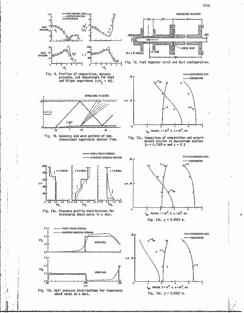
10-25

1.0 -EDDY BREAKUP MODEL 0 DIMENSIONS IN METERS-..--CO PLETE REACTION "

N8- 0 EPRMN . 8 61 10o20

.30 .6 0 z

MASK M 2.99 NOZZLE 0

FRACION 4 T, .4)

02

.1O LOP'F , I X 0 .7369 ,

oFig. 12. Fuel injector strut and duct configuration.5 0 I 2 456

Fig. 9. Profiles of composition, dynamic 0W EXPERIMENIAL DATApressure, and temperature for Kent - COPUTATI(Nand Bilger experiment (x/d. 40). Ge J0

TDIMENSIONS IN MEERS

/fr/ . ,LL zm .01

/

.10 803 .7369

S I II1 0 1 1 1 Fi g . 1 2 . F e l e i PeRCENT. t x 10 nd K d u xc1n" ga t

Fig. 10. Geometry and wave pattern of two-dimensional supersonic channel flow. Fig. 3a. Comparison of computation and experi-

mental results at downstream station(x = 0.736g m and y = 0.).

-SINCIO FITTING PRGRAM

---- ARAm.ICMARHIN PRQTA1~ 0 E' EXPR IMENTAL DATA

.002

.... PARA~tlCAV, CHIN PR M,', , -CMPUTATION

Z0.023 0'00~i

.016 X 00 45m

/{. . . 05 1 T,

Fig. 11a. Geoetry andofie patrun f o- Fig l Cmaio fcmptto nxeidimnsional supon avsinc cane flow. me'Cnt reut a downsrea ,uxI0 . staio

Fig.736 m y 0.00)m.I.~SHC 6IIN PROGRAMTIN POGA

-.-.-. PARABOLIC MARCHING PRORAM .0 }3C V RIETLDT

j.01 \ i

PIP o pipe PI1

S !Fig. 11 al pressurpoe distributions for 0ans2e3se

i .sock ave in duc, Fig. 13c. y = 0.0063 m.

I>

Y.M 4~M 01

.04

11.2--------------------------- .0OWER WALL 1,6

03.03 0 1 2 3 4 5

Fig. ll. WalPressurpoe distributions for asee .PECT.2 .u12

itravrs shockewav s in a duct. FHg. PERCEN. T x 10K.02 m. I

.0 0 0 > EXPER IMENTAL DATA

.T--OMPUTATN 300 EXPERIMENT0

- COMPUTATION

..01

0 02.0 0

00

M0 1 3 4

iae. PERCENT. I x l0". K. U x I0"2. mIs

Fig. 13d. y -0.0063 m. 1.0 -

000 0

00 EXPERINENTAL DATA

.02 - COMPUTATION

! U' I I Il

0 1.0 2.0 3.0 4.0ai.01 -Y(M ,, ,o y (cm),

I -Fig. 16. Comparison of Mach number profiles forsupersonic combustion of hydrogen andvitiated air (z 35.6 cm).

0 I 2 4

It , PERCENT. I x 1 r" , x w0 , mis

Fig. 13e. y = -0.0127 m.

Y

y I I

M= 2.44 0.476cm TOTAL HEIGIT T &9cmA.0. 400cm OPEN HEIGHT I04 ~

AA .:--35.6 cm-HZ A-A IIA- AA1.5

H2Fig. 14. Sketch of test section of combustor duct.

1,.0 EXPERIMENT

0 1.0' .8 002 0

0 N2 0

.A H20 TilT ref 00,.6 '" -C OIPUTATION 0-

VOLUME FRACTION 0OFSPECIES

.5

0 EXPERIMENT

. COMPUTATIONT ref =2380 K

I I I

0 1.0 2.0 3.0 4.0y zo com .o ,t y(cm)y~ (cmM)

F'q. 17. Comparison of stqnation temperatureFig. 15. Comparison of composition profiles for profiles for duct6d supersonic c;'m-

ducted supersonic combustion of hydro- bustion of hydrogen aid vitiated airgen and vitiated air (z = 35.6 cm). (z = 35.6 on).

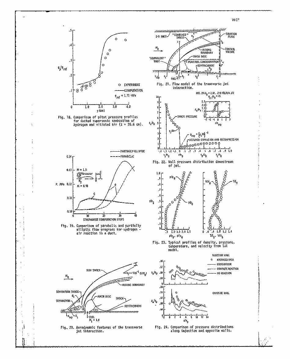
10-27

0S H C K I -P L A E

(0 MIXING CORO0BOUNDARY I VLPt

0 QUIVALNT' / MACH DISC.3BODY-.. PEAK FUILCONCENTRAIIOI ZK

0REATTACHAIENT z.p ref L__

.2 ~Sep Fu fuL'

- EXPRIEN Fig. 21. Flow model of the transverse jet0 COPUTAIONinteraction.

-J9 -2.5o 1.0 2.0 3.0 4.0 1.S-01

y (cm) , 3 I) .

Fig. 18. Comparison of pitot pressure profiles 6 SHOCK PRESSURE afor ducted supersonic combustion of C6/" .3 -2 -1 0 1 2 3hydrogen and vitiated air (z =35.6 cm). P"Ipa C3 Vep

p3(fr~ exp [P2 rASSLVAED EXPANSION AND RECOMPRESSION

0 6 0 0 oE~31 0000I 1 0? T

- PARTIALLY-ELL!PTIC -4 -.3 -.2 -.1 0 .1 .2 .3 .4 .6 %7 .8 J9 1.00.14 -- - -- PARARC.;C XROO Io 1 Y

Fig. 22. Wall pressure distribution downstream/ of jet.

0.13 -M- 1. 5,

P. MPa 0.12 - H2 a 00[ V 0.\ Tito

c.6 -0

4 -00 6

0. 10 LA3

0 10 20 30 40STREAMWISE COMPUTATION STEPS .2 A

Fig. 19. Comparison of parabolic and partially . . .elliptic flow prograins foririydrogen - 5 1.8.520 .air reaction in a duct, . 1.0 .5 20 2.5 ~ ~ 0 iv0

Fig. 23. Typical profiles of density, pressure,temperature, and velocity from TJ1model.

INJECTION WALL

.160 ANERAGED DATA- EQUILIBRIUM

.12 -COMPLTE REACTIONBOW~PW9 SHOC -11 M ~~ 3 0 - NO REACTION

..........

MIXING BOUNDARY .20 -

SEPARATION SHOCK .16 - 0 OPPOSITE WALL

SEPARATION SHOC P0 P 00 8 0~REATTAC1WAINT W .

.... .... .... .... .... .... ....

Sep.S..6 0 2 4 6 8 10 12 14

AFig. 20. Aerodynamic features of the transverse Fig. 24. Comparison of pressure distributionsjet interaction, along injection aiid opposite walls;

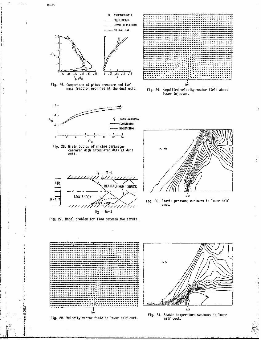
10-28

0 AVERAGED DATA ____

- EQUILIBRIUM --. . -..... - .

-- -- COMPLETE REACTION -- -------

.o.... . NO REACTION - -

z% . L~-- -- -- --- ----------------------------....--- :::::::f.----.----------- ----------

.o .1 .... .. ..o .=. . : ::: L:!i :........... '" ".... ...... A.. . . . . ....... .....

Fig. 25. Comparison of pitot pressure and fuel SLOT

mass fraction profiles at the duct exit. Fig. 29. Magnified velocity vector field about

lower injector,

.6 -..................... .... . .................

.46

m INTEGRATED DATA

2F E QUILIBRIUM

............ NO REACTION

0 2 4 6 8 10 12 14

Fig, 26, Distribution of mixing parametercompared with integrated data at duct 71

exit.

H2 M czI

AIRA_ REATTACHMENT SHIOCK

M. BOW SHOCK :7- Fig. 30. Static pressurc contours in lower half

-~j -- W S-7--duct.

SH 2 M.-I

Fig. 27. Model problem for flow between two struts.

-T K

,_.,, /

.............

/

,j 3:'ZS"LT' Fig. 31. Static temperature contours in lower

Fig. 28. Velocity vector field in lower half duct. half duct.

10-29

0.3 0 DATACALCULATION

,0.2-

.oI0.1

0 0 0 0

50---.50 1O 150 200

SLOT WIDTHS UPSTREAM OF SLOT

ROT Fig. 34. Comparison of exp. rimental and calculated

Fig. 32. Hydrogen mass-fraction contours in hydrogen mass fractions along plate.lower half duct.

4

0 DATACALCULATION

3PWP0 0

2 010

0I I I

0 S 00 200 300 400

SLOT WIDTHS UPSTREAM OF SLOTFig. 33. Comparison of experimental and calculated

static wall pressures.

t1

10-30

DISCUSSION

F.C.Lockwood, UKThe shock-induced'separation zo-,e is very dependent on the quality of the predictions for the.'pinging shock. Howprecisely do you manage to obtain the required good definition of the shock %ave ,itlth a finite ifference tedinique.

Author's ReplyActually, the low shock preceding the upstream separation zone (Fig.28) does not-impinge on the lower wall, theshock is intitiated near the lower wall as'a result of main stream flow blockage by the transverse jet (see page 10-9).All shock waves including the low shock are captured using the present technique. The capturing technique resultsin theshock being smeared over several node points; however, the jump conditions associated with each shock aresatisiled although the conditions behind the shock are spatially displaced somewhat. We do plan at a later date toreplace the present scheme with a shock fitting technique (see pages 10-18, 10-19). The fitting approach would moreappropriately treat shocks as discontinuities.

3.H.Whitelaw, UKIn the first example you discussed the flow has Ma > 1 in the stream and Ma = 0 at the wall. You solvedparabolic equations throughout. Did you have any difficulties in the near wall region. In the second example, youpresented results and said that'the "basic flow conditions have been predicted". What does this phrase mean inquantitative terms, bearing in miid the discrepancies mentioned earlier by Dr J.M.Guirk in connection withisothermal, two-dimensional jets in mass flow.

Author's ReplyIn the first example discussed during the oral presentation, we had no noticeable problem in the near wall region ofthe duct. No data wereavailable very near the wall, and no data comparisons were attempted there (see Figure,3 15,16, 17 and 18). To resolve steep gradients near the wall without using a large number of grid points, wall functionswere used to define fluxes at near boundary grid points (see pages 10-6, 10-7). Therefore, the parabolic equationswere not applied very near the wall where elliptic effects could be present.

The second example discussed during the oral presentations was intended to be qualitative as no data were availab!efor comparisons (see page 10-17). The third example presented a quantitative comparison of elliptic code resultswith data. The basic flow conditions discussed in the talk and written paper referred to the separation, bow, andreattachment shocks, and the recirculating regions lying ahead of-and behind the shock (see page 10-17). Thesephenomena were in qualitative agreement with experimental observations from a configuration similar to the strutflow model problem (Fig.27).

H.Wilhelmi, GeWe published local concentration measurements for transverse fuel injection into supersonic flow (cf. It.Wilhelmianl G.Gross, ir: Turbulent Combustion,.Prgress of Aeronautics and Astronautics, LKennedy ed., New York1978, pp.3 11/27). in this work, it was shown that also for supersonic flames the data in the mixing and reactionregion can be correlated by a normalized error function with a high degree of atcuracy. Susprisingly this even holdsfor regions of the slow field that are crossed by oblique shock waves. The experimental values yielded smoothcurves for the values of constant concentration with a steadily increasing half width of the jet in downstreamdirection. These results did not show the inflection points and the maxima given in Figure 32 of this computationalwork. It is possible that these differences are due to the grid chosen for the computation, to the sunming tip oferrors and to the turbulence model used..

Author's ReplyWe believe the inflection point in the 1 percent contour line of Figure 32 is likely to be numerical in origin. Thedownrunning bow shock from the, upper injector passes through the contour line at approximately this point. Mildoscillations of the dependent variables near a strong shock is typical with the present numerical techniques, andthese oscillations would be most-obvious with low hydrogen mass fractions. The velocity vector also turns down-ward as it passes through the downrunning shock, changing the streamwise component -for hydrogen convection.This change !ay also affect the orientation of the contour line. We believe that the maxima present in the 25, 50and 75 perc nt contour lines are a-function of the strength of the hydrogen jet, as compared to the strength of theair cross flow. The maxima'were more pronouncedwith higher jet strength?, we have.not considered any lower jetstrengths than those presented in~this paper.

It is of course possible that the present turbulence model introduces inaccuracies and the chostn grid may notaccurately resolve the very high gradients close,.to the fuel injectors. The turbulence model is considered only aninterim solution to the complex turbulence field that mustbe modelled. We are also considering other means foroptimizing the discretization (floating grids, rnulti-grid s.hemes) and utilization of the STAR 100 vectoi computerai Langley'Research Center to allow mgre modes to be used.

|l-!

DEVELOPMENT AND VERIFICATION OF RADIATION MODELS

H. BARTELDSInternational Flame Research Foupzation

IJmuidenThe Netherlands

Present affiliation:TNO Organization for Applied Scientific Research

Division of Technology for SocietyP.O. Box 342

7300 AH ApeldoornThe Netherlands

SUMMARY

The prediction of radiative heat transfer from a flame may be divided into three catego-ries:

1. the evaluation of temperatures and radiating species concentrations,2. the evaluation of the absorption-, emission- and scattering characteristics

of the species at the prevailing temperatures,3. the evaluation of the radiation exchange.

Models falling into category 2 and models falling into category 3 have been developed.The models have been verified by comparison with measured radiation intensities andmeasured radiative heat fluxes from relatively large gas flames.

As input to the models measured temperatures and species concentrations hae been used.However, the models are well suited to be combined with each other and with predictionprocedures for fluid flow and combustion.

DEVELOPPEMENT ET VALIDATION DES MODELES DE RAYONNEMENT

RESUME

La pr6diction du transfert de chaleur rayonnante a partir d'une flamme peut se diviser entrois categories:

1. Evaluation des temperatures et des concentrations d'espbces rayonnantes,2. Evaluation des caract6ristiques d'absorrtion, d'6mission et de diffusion des

espbces aux temp6ratures r~gnantes,3. 6valuation de l'change radiatif.

On a mis au point des modules appartenant aux 26me et 3bme cat6gories. Pour valider cesmodules, des comparaisons ont 6t6 effectuees avec les r6sultats des mesures d'intensit6de rayonnement et de flux de chaleur rayonnante 6mis par des flames gazeuses de taillerelativement importante.

Les mesures des temp6ritures et des concentrations d'espbces ont 6t6 incorpor4es aux mo-

dbles. Ces modules peuvent tre combinds ensemble et se pr~tent bien aux proc6dures deprdiction d' coulemen-, fluide et de combustion.

LIST OF SYMBOLS

a weighting factor, black body factor in specified spectral regiona subscript, referring to absorptionb subscript, referring to-black body radiationbc collision half width mb constant in polynomialb in constant in polynomialb 3n constant in polynomial K- 3

b 4n constant in polynomial K 3

c velocity of light mic concentration of soot g.m 3

c subscript, referring to carbon dioxideco subscripts, referring to carbon monoxide,f photon density m3s

gV subscript, referring to gas2h Planck constant W 2

I ifntensity of radiation integrated over electromagnetic spectrum Wim-2 -I V intensity of radiation .,t frequency v W.m .8I intensity of adiation at wavenumber w W_K absorption/attenuation coefficient in 1

gray gas/(averaged) specific spectral absorption coefi.cient m, bqrk gray gas/(averaged) specific spectral absorption coefficient m.bm number of gray gases/number of spectral regions

11-2

M subscript, referring to methanen number, referring to gray gas or spectral regionn unit vector in the direction of pencil of radiation beams -

P total pressure barp partial pressure ba 1S integrated spectral absorption coefficient m .bar-

s subscript, referring to scattering, source or sootT temperature Kw subscript, referring to water vapourX length of column of gas mx, y, z Cartesian coordinates mz, r, 0 cylindrical coordinates m, m, -

a absorptivitya sclid angleY, spherical coordinatesA indicates small increase/decreasee emissivity

wavelength of radiation m_1v frequency of radiation sa 3.1141592654Z summation conventiona Stefan-Boltzmann constant, .567 x 10-7 WP-2.Y "-1

wave number of radiation mV differential vector operator m

1. INTRODUCTION

Efficient use of energy, low pollutant emissions, low capital costs, while the processrequirements are satisfied, are dem.is on combustion installations. Problems concerningflow, mixing, combustion, heat flux distributions and pollutant emission levels have tobe solved for an optimum design of a burner/furnace combination. The ultimate universalsolution to these problems can only be via the route of mathematical modelling techniques.Wide gaps exist in the computational development of these models and the physical andchemical information required. Furnace trials have been executed to obtain informationon the physical and chemical processes occurring inside furnaces [1, 2]. The obtainedinformation has to be generalized via mathematical models. In this paper mathematicalmodelling work concerning radiative heat transfer will be reported.

Tne prediction of radiative heat transfer froi a flame may be divided into three catego-ries:1. the evaluation of temperatures and radiating species concentrations,2. the evaluazion of the absorption-, emission- and scattering characteristics of

the species at the prevailing temperatures,3. the evaluation of the radiation exchange.In the present paper all three categories will receive attention both with respect toexperiments and mathematical models. However, more detailed information will be presentedconcerning the development and verification of radiation models falling into categories? and 3.

2. TEMPERATURES AND RADIATING SPECIES CONCENTRATIONS

Before a radiation model can be applied it is necessary to evaluate the temperature dis-tribution and the radiating species concentrations throughout the flame. The temperaturefield and the concentration fields can be obtained in different ways ranging from thepractical experience of the combustion engineer to a more fundamental approach sol.vingdifferential balance equations for mass, momentum, chemical species, enthalpy, etc.The latter approach has been investigated with varying success 13, 4, 5]. One can calcu-late furnace performance to a certain degree of accuracy for gas flames, however forheavy fuel oil- and coal flames complications occur. The determination of the concentra-tion field of soot particles and the assessment of the radiation characteristics of sootparticle clouds are very complex subjects, which are only mentioned briefly. The resultsto be presented refer to gas flames. The models, however, are not restricted to gasflames; coal- and oil flames may be treated by these models without too great difficul-ties.

For our purpose, the verification of radiation models, it is not possible to rely ontemperatures and concentrations obtained in aforementioned wa,,s. The verificatiou ofradiation models is best done in isolation. Therefore as input to the models measuredtemperatures and species concentratlons have been used.

3. RADIATION CHARACTERISTICS OF CHENICAL SPECIES AND SURFACES

Radiation characteristics of the chemical species in a flame involve absorption-, emis-sion- and scattering characteristics. Lowes and Heap [6] have shown that scattering forscot is negligible and scattering for large coal particles is forward directed. Conse-quently to a first approximation scattering can be ignored in luminous flames. Certainlyscattering is not very important in gas flames. Therefore we will mainly concentrate onabsorption and emission.

The basis of all methods for the solution of radiation problems is the equation ofradiant energy transfer, which is derived by formulating a balance on the monochromatic

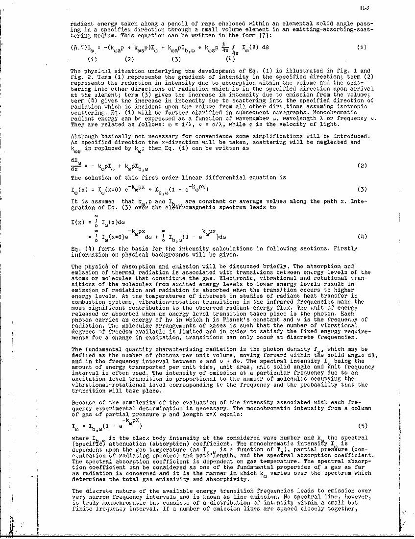
11-3

radiant energy taken along a pencil of rays enclosed within an elemental solid angle pass-ing in a specifiea direction through a small volume element in an emitting-absorbing-scat-tering medium. This equation can be written in the form [7]:

(fi7)1 =-(k ap+ kwsP)i e + k aPIb, + kwsP I_ f I (a) dS I

( )(2) (3) (4)

The physial sitoation underlying the development of Eq. (1) is illustrated in fig. 1 andfig. 2. Term (1) represents the gradient of intensity in the specified direction; term (2)represents the reduction in intensity due to absorption within the volume and the scat-tering into other directions of radiation which is in the specified direction upon arrivalat the alement; term (3) gives the increase in intensity due to emission from the volume;term (4) gives the increase in intensity due to scattering into the specified direction ofradiation which is incident upon the volume from all other diretions assuming isotropicscattering. Eq. (1) will be further clarified in subsequent paragraphs. Monochromaticradiant energy can be expressed as a function of wavenumber w, wavelength X or frequency v.They are related as follows: w 1IX, v = c/lX, while c is the velocity of light.

Although basically not necessary for convenience some simplifications will bt introduced.As specified direction the x-direction will be taken, scattering will be neglected andk is replaced by k ; then Eq. (1) can be written as

dIdx- k pI + kp! (2)

The solution of this first order linear differential equation is

IW(x) = I0 J(x:o) e-kWpx + Ib,w(0 - e-k pX) (3)

It is assumea that k ,p and I are constant or average values along the path x. Inte-gration of Eq. (3) over the elecromagnetic spectrum leads to

I(x) I k (x)dw0W

-k px kDxI (x=O)e kWP dw I I (1 - e 0)' (14)

0 W ~ o b,woEq. (14) forms the basis for the intensity calculations in following sections. Firstlyinformation on physical backgrounds will be given.

The physic of absoiption and emission will be discussed briefly, The absorption andemission of thermal radiation is associated with transitions between entrgy levels of theatoms or molecules that constitute the gas. Electronic, vibrational and rotational tran-sitions of the molecules from excited energy levels to lower energy levels result inemission of radiation and radiation is absorbed when the transition occurs to higherenergy levels. At the temperatures of interest in studies of radiant heat transfer incombustion systems, vibration-rotation transitions in the infrared frequencies make themost significant contribution to the observed radiant energy flux. The unit of energyreleased or absorbed when an energy level transition takes place is the photon. Eachphoton carries an energy of hv in which h is Planck's constant and v is the frequenjy ofradiation. The molecular arrangements of gases is such that the number of vibrationaldegrees if freedom available is limited and in order to satisfy the fixed energy require-ments for a change in excitation, transitions can only occur at discrete frequencies.

The fundamental quantity characterising radiation is the photon denaity fm, which may bedefined as the number of photons per unit volume, moving forward within t e solid ang.Le da,and in the frequency interval between v and v + dv. The spectral intensity I being theamount of energy transported per unit time, unit area, unit solid angle and nit frequencyinterval is often used. The intensity of emission at a particular frequency due to anexcitation level transition is proportional to the number of molecules occupying thevibrational-rotational level corresponding tc he frequency and the probability that thetransition will take place.

Because of the complexity of the evaluation of the intensity associated with each fre-quency experimental det.rmination is necessary. The monochromatic intensity from a columnof gas of partial pressure p and length x=X equals:

-k pXIW = Ib (I - e (5)

where I W is the blac4 body intensity at the considered wave number and k the spectral(specifh attenuation (absorption) coefficient. The monochromatic intensivy I isdependent upon the gas temperature (as I is a function of T ), partial pressure (con-oentration cf radiacing species) and patMIPength, and the spectral absorption coefficient.The spectral absorption coefficient is dependent on gas temperature. The spectral absorp-tion coefficient zan be considered as one of the fundamental properties of a gas as faras radiation is concerned and it is the manner in which k varies over the spectrum whichdetermines the total gas emissivity and absorptivity.

The diacrete nature of the available energy transition frequencies leads to emission oververy narrow frequency intervals and is known as line emission. No spectral line, however,is truly monochromatic but consists of a distribution of intensity within a small butfinite frequerc interval, If a number of emission lines are spaced closely together,

- - . -z~ - , % . . .. . . . . . . . . . . . . . . . . . .. .. .I ,_.. .... . . . . m - " . f & z .

114

they may in some cases overlap; then they cannot be considered in isolation. Radiationfrom overlapping lines is known as band radiation. Although such bands are composed entire-ly of absorption-emission lines, the discrete band structure is commonly ignored byaveraging over frequency intervals which include many lines.

The transition from one energy level to a lower level ideally occurs at a single frequencybut in practice the emission line is broadened and spreads over a range of frequenciesabout the transition frequency. There is a natural line width that is the result of Heisen-berg's Uncertainty Principle (natural line broadening), while broadening of lines can becaused further on by the perturbation of energy levels- due to collision (collision broad-ening) and the thermal motion of the emitting and absorbing species relative to the ob-server giving a shift in the apparent frequency (Doppler broadening). Of these mechanismscollision broadening is the dominant broadenihg -iechanism for most furnaces and combustionchambers but Doppler broadening becomes important at low pressures such as those encounteredin rocket engine exhaust plumes at high altitude; see Hottel and Sarofim [8].

The distribution-of absorption coefficient about the line wavenumber w is given for acollision broadened line by Penner [9], Tien j10] and Hottel and Sarofdm [8].

S bk W (W _ W + bc (6)

0 cwhere S is the area under the k - w curve for the broadened line and is called the inte-grated line intensity; and b i the collision half width for the line, fixing the poai-tion at which k falls to haif its maximum value.

The intensity of radiation leaving a volume of gas due to emission from a single line canbe found by integration of the spectral intensity over the entire spectrum.

I I 0,(1 - e )dw (7)

In most gases of practical interest the emission lines do not occur in isolation, but arespaced so closely together that the broadened lines overlap to . considerable extent. Whena number of lines overlap the specific absorption coefficients are additive, and the con-tribution to the intensity of radiation from the entire band can be found by integrationbetween the frequency limits of the band.

032 -k pXI = I (1 - e 0 )dw (8)

The spectral absorption coefficient ke represents the sum of the absorption coefficientifrom the considered lines at the wave nui~ber w.

The total gas'emission can be found by integration over the entire spectrum. The totalemissivity of a gas at temperature T is equl1 to the ratio of the emission by a gas layerof length X to the black body emissign at temperature T

00-k(Tg)pX]Ig I Z (T )[I - e ' dw T~X

:g bLW M f (TpX (9)1Ib (Tg)dwo 'biw g

In a sLidlar way the to.al gas absorptivity can be evaluated, but in this case the distri-bution of energy in the spectrum is related to , 'temperature at which the intensity,absorbed in h certain gas layer, is emitted.

C -k (T )pXI (Ts [ - e W g ]dw

:g = 0 : b~' f (Tg,TsPX)Ib (Ts)dw

0 'b,w swhere I (T is emitted at a source temperature T and the spectral intensity is depen-dent on

t'nisSjource.

In Eq. (i0) f is considered to be due to a black body mitter. However, the sourcedoes not have-$t be a black body !or gray body). The intei slty can be due to e.g. a gaslayer having a certain composition- and temperature distriUition. The absorptivity thenbecomes:

0 -'k (T )pXI t (Ts)[I - e w dw

'g : d f (Tg,TspX) (11)egs

I(Ts)dw

Now the source temperature does not have to be a constant but can be a temperature uistri-bution. The distribution of the spectral intensity can be very complex in this case.

A number of modelB have been proposed to avoid the problem of for-mulating the attenuationcoefficient as a complex function of wave number. The purpose has been to provide a modelof the relative spacirg and intensity of lines in a band. Such a i.c-el combined with asuitable description of the line broadening function leads to an analytical solution ofthe intensity of radiltion from a band. Among the proposed models are the Elsasser, theMayer-Gooey or statistizal model, and the tox molel devel6ped'by Penx.er t9]. More informa-tion about these mode14 can be found in Johnson [11], Tien [10] and Aottel and Sarofim [8].

A fundamental approach cf the emission/absorption problem must take act-unt of the spectral

Lpc

! 1-5

nature of gas radiation, but the problems involved in handling the spectral. properties ofthe gas mixtures are enormous, so in many cases the problem is handled by using measuredtotal radiation properties. Total water vapour emissivity and carbon dioxide emissivitycLarts in which information from several sources is used are presented in Hottel and Saro-fim [8]. Johnson [11] discusses these charts and mentions more recent publications in whichthe regions, where the above-mentioned charts are less accurate, are indicated. However, atthe moment the recognized standards for evaluating total emissivities of water vap:ur andcarbon dioxide are these charts. Hadvig's charts [12] for total emissivities af watervapour/carbon dioxide mixtures are based on the charts in Hottel and Sarofim [8]. Lee andHappel [13]hare measured emissivities for methane. Hottel and Sarofim [8] present a charton the total emissivity of carbon monoxide based on the measurements of Ullrich [14].

In furnaces the gases normally are compcsed of two or more radiating components. For a mix-ture of two gases the total emissivity equals:

-k p+ k p)X2 Ib[1 - e -( , ,2P2)]dw

I1 dw0 b,w

eb [(1 - e-k ' Ip lX ) + (I - e-k 2 P2 X - --kW'P 1 X XI - e-k ,2P2X )]dwoC

+ 2 - +2 bw (12)

The emissivity of a mixture of two gases is equal to the sum of the emissivities of thetwo gases minus a cori.ction for spectral overlap. If there is no spectral overlap thecorrection factor equals zero.

Fig. 3, taken from Johnson [11], presents an idealized distribution of gas spe ral ab-sorption coefficients for H 0, CO , CO and CH,. It can be seen that overlap occurs in someparts of the spectrum so corectigns are necesary. It should be realized that the absorp-tion bands are comj.ztsed of series of spectral lines close together and that these spectrallines are affected by temperature as can be seen in fig. 4, which is based on Lee andHappel [13]. The spectral absorptivity for the 2.37 pm band for methane i.. shown in thisfigure. For the absorptivity o (see Eq. 10) of a mixture of carbon dioxide and water vapouran approximate evaluation can ge made by using the relations given by Hotel and Sarofim[8].

T 0.65 Mcc (Tg3sT5 pX) = (T c (TspX ) (13)

0.45 T(T 'Ts'PX) = (-A) w (TslPX !T) (14)

cw -c S~ w T wc 04 c + ccw - AV.c+w (15)

Ac is the correction factor for spectral overlap. These absorptivity' formulations canbecuved if the radiation intensity is black body radiation from a surface at Ts . However,in a watercooled furnace with low wall temperatures the radiation from furnace walls isnegligible and all the radiation within the enclosure is from gas radiation, which is notby any means black body radiation.

Combining Eqs. (4), (9) and (11) for X = x one arrives at0O -k px 0' -k px

I(x) I I (x=0) e d I (1 - e )dw0o0 c ob(1 - a ) I (x=O)dw + c I dw

go 0W g o b,w(I a ) I(x=0) + C I

(1-a) I(x=0) + E 9 (16)g g i

So the intensity I(x) in x-direction is composed of a transmitted fra.tion of I(x=O)through the layer x plus a part emitted in she layer x. In Eq. (16) I is the integratedblack body intensity of the gab at temperature T , while a is the Steran-Boltzmann constant.When the intensity I(x=0) originates from a turfgce, as is often the case, one needs toknow the radiative properties of the surface.

The radiant energy interchange within enclosures is affected by the radiative prope-tiesof the surrounding walls. To analyze the process within a furnace enclosure it is necessaryto know the emission, reflection and absorption ?roperties of the walls as the temperaturelevel and -distribution in the gas volume is affected to some extent by these properties,while the heat transfer and heat transfer distribution to cooling loads are strongly in-fluenced by these properties. Only radiation properties of black bodies are well estab-lished. The walls in Zurnaces normally do not behave like black bodies. The emissivity offurnace walls and tubes is a fuaction of direction (angle of emergence), wave length andtemperature; the imp~rtanca of these parameters is influenced by the surface condition.Factors like roughness, oxice layers and physical and chemical contamination ar' used toJI describe the surface condition.

11-6

The el ectromagnetic -theory can'be used for a fundamental approach to the radiative proper'-te f, surikaces. Howeve.r, 'the surface has to bi vTi~1'y well defined for a theoretical-

treatment; it has, to be' optically tjrdboth, physicall5- and chemically clean to allow a pre-diction of the monochromatic reflect~nce in. thc, ibeular direction to be made. Fu'rnace

*wall.s" and tubes ie .noizlly p6t, well enough ddfihed' for a theo'retical treatmeht; ae-6sitsof combustion pfdut onteiah hange the 6hiraeitc oth ilsdring opera-tioni. Measured'data, have to be used to obtain th6, neicessary knowledge about ihe surface-behaiviour. For meitalic surfaces the emissivity fS's~wn with wave lengt;'the emissivity

*of iron and steel can vary, fxiii .abov& .8, to below A-5 bbt'ween' .2 and 10 pim., Refraetoryjmaterials can have, a st, ong, vrnito r6f lmsiiy ih a ength;, -several tinim anmaxima-~can appear over the- spa'trl'mn. Th angular distr'ibutions of enissivity, for ntliand refractorynmaterials area hot the same. For small angular inclinations 'relative' to the

norml onthesurfce te ei*:ivity of m'etallic suirfaces-is. quite- constant; with irireas-ing angles the emissivity ir reases quite sharp And the emissivity falls down to zero whenthe inclination angle dpproach~e, 90.Refragtory ma,8erials' show a slight decrease indmissivity for' inclinati6n arigles between 0 and 60 '; for higher angles the decr,''se is

I sharper with the 6missiVity Opproaching 'zero when the inclination angle equals 90!.

Although quite a lot of infi',ation on surface radiation is available in the .literaturp* I e.g. in Perry [15], Sparrow.-Prid Cess [16], and Hottel and Sarofim [8], niot very much is

known concerningthe radiati've'b:ehaviour of furnace walls, under combustion conditions.N~ormally one relies, on to~tal (,integrated oveir the spectr'um) hemispherical (in'tegr~t~dover all- angles in -an hemispr-e) e'missivitie-6obtained from the literature. For ir~on and

se 'with diffe'enf 6rfa~e cbfiditibfi . e'~t~ .0 n 9 a e found. Theemissivities of refractory materials, of i~h. 'e grain structure is~ an importanit para-meter, vary between _25 and .95.. The effect of wall temperatures on the absorptioi'coefficient for different furnace we-ll materials'is shown in fig. 5, 'taken from, ',h Kuijkand Spagnjers [171.

Toor and Viskant'a (18,. 1,4) have studied the effect of radiative properties- of surfaces onthe radiant ieat transfer between surfaces. They conclude that 'for an'-aciirate 'pr~dictionof lcalj irradiation the directional'oharacteristics must be -considered while calcula\tionof thd irradiation on -a non-gray basis does not yield improved results over a gray aha-lysie". In furnaces &,hese conclusions could loose'thei'rvalidity to some extent"as betweenthe ' a-vs gases radiate. The gas'radiatioh is s6trongly dependent on' wave length, so theabsorpt~tvity' of the -walls, in the spectral regions, whiere gas emission is high,, can be veryIim ortal t. In 'analyzing the radiative heat trandf er. within -a f urnace enclosure, the totalemissi Vity-.6f refractory s6rfaces. is normally, assumed to be about .5 while th6 totalemissivity of steel, tubes 'is assamed 'to be above .-8.

As will be clear from this section for practical emission/absorptiuh models one needsito

simplify. This will be done in the next section.'

4i. EMISSIONZAMSC.RPTIOW MODELS

in this section a number of emission/aborp~tion models, for th.e 3rediction of radiatioiin--tensity wi'll be developed.

A: Gray gas models

If the variation of the absorption coefficient 'K(=kp) with 'spebti..a position, partial1pressure and temperature 'is, heglected and a mean- value f~O bith6 Abiorition coef ficient Kis usedi Eq. ('16), c~h 'be writ ,ten as

-Kx c~T ~ -KxIh tY.e th !(=om I sv

i Yegray g~s model temksity equals the absorptivity

pd ;'! ;h x. hechoceif te a Isoptin -o&, fi~e-6 Kba tdb _based on" the' combustionpraw~t (i ou ex-erm~ts kon' nturl.'as) te 'verge, i~thingt, (furnace dimensions)

'a emfperatires. Theichosen-v'alue ar I in tablo- I.

tal i ostnsof jgr.y Kap' m6dels "for tlhe ~d go ehn combustion

B: Orp clear/two gray gais model

j X~A better way, to represent the enissiVi1ty of a real ,gas. is to, take the sum of the weightedte 'fone cl' ar'and-- two gra . - I instead of using one gray gas. (9

'g,n 'n+b?n '

414

Theweighting factor a can be considered 's the quotient of the spectral black bodyintensity integrated o& the Wave number region where k, = k (= constant) and the spec-tral black body intensity integratedover ,the complete s~ectrUm. Then

a - = 4, (21)

and Eq. (19) follows from Eq. (9) and Eq. (16) can be written as the sum of three intensi-ties, each represeniting a part of the spectrum-

.3 3 -k-Px -'k xTI (x) = l In(X) h [In(x=O) e ag,fi(Tg),l , n (22)

The factors of table II have been determined, by Johnson [Ii such that Eq. (19) closelyfits to measured emissivity/pressure pathlength eiationships for th combustion productsof methane combustion. The emissivities based on measuhementsfare given in Hadyig's charts

[12]; 99 data points have been used.

table II: constants of one clear,/two gray gas model for the products of methane combustion

n b In b2n,-0 kn

" +.255 +.-26k 0.002 +.500 -.157 1.833 +,,,24i5 .103 32.30

The clear gas with k = 0.00 corresponds to the weakly- and non-absorbing parts of thespectrum. The partial pressure p has to be taken as the sum of the partial pressures ofthe radiating gases (mainly carbon diodde and, water-vap6r).

With this model themaximum discrepancies be tween, qmissivities using Eq. (19) and'measuredemissivities amount bout'10% for partial pri'ssc pathlengths (px's) between .02 and1.5 bar.m. Due to the clear gas thdimaximum evils,1xities at infinite pathlength for tem-peratures between 1000 and 2000 K are i'estrited- o, too low values. The maximum emissivi-ties are on average lower than the measured' emis yiti'es' at a pressure pathlength of1. 2 bar.m, while at this- pressure pathlength Eq. '(19)- underpredicts emissivities by about10%. This means that the ,-a'del 'ith the constants oR table II becomes increasingly inaccu-rate if the mean pathlength isrlarger than 4- in for a natural gas flame ,with a partialpressure of carbon dioxide and water,vapour of rough'y 0.3 bar. For large furnaces themodeX seems to have deficiencies.

C: Four gray Sas 'model

A more accurate calculation of emissivities can be obtained withthe following formulationsi knPX

Cg ,n~1 n (T-)(1 - e ) (23)

a ' g~= 'bh +ba6 T '+ bn 2~ + b~ TY (24)

We have chosen a, larger punfber of gray gases and-a higher order of the polynomial thanbefore to ascertain that the emissivity, can be deter.iined very accurate. The clear gashas 'been dop'pedto pre'ient the aforementioned problems at longer pathlengths. The con-stants bf table III have been detEL'mined by fitting- Eq. (23) against the same jritsuredemissivity data as used, fr the pl vi&us model.

tble,III: constants of four gray gas model for the products of methane combustion

n .1 b 03 b - "0 b n'109 "

I .i-+ +.065 -.026 0.1i06

2 -:.535 -.240 +.009 +,.002 1.6533 +;,131 .089 -.127 +.032 21.2124 +.16 132 +,053 -.0081 A46.308

The fit was made; over the temperature iang( of 'J000-2000 K An'1a ap,'tial pressure pah-length range of 0.003 - 1.2'bar.m. The cmissiv'ty calcAiation. os very good as the aderagedeviation from measured emissivities is less--th6n. 1% over tAe- above ranges.

In table IV the weighting factors andthe absorptioh coeffi.ients are given for t la fourgray gases.

table IV: weighting factors and absorption coefficients of' four gr6-j gas model f ;r the': ] pr6ductsof methane combustion

1o000 K 1200 K 1400 k 1600 K 1800 K -2000 K 1000 - 2000 F

al .540900 ,607500 .672000 .733100 .789600 .840200 k .106i65a2 .304100 .261200 .219300 .178300 .139300 .01300 1,: 1.6528(0a- .124900 .109900' .093870 .-078390 .064960 .055120 '2 21.2120,0aa .029980 .021390 .014810 .009851 .006139 .003296 k46308060

'P4 .. 4,-'- ~~ -

Radiati6i-intensities can be calculated, using Eq. (22) with-n from I to A.-

D: Spectral model

Representing a real gas by a series of-graygases for emissioin/absorptioh purposes misre'presents s6me physical realities. The-waVe lehgth iange in which emission occurs and'themonochromatic euission/attenuation coefficients vary with gas temperature. Some radiationemitted at-high temperature cannot be attenuated by gas ata low6r temperature. The change

inmonochromatic emission/attenuation coefficients With temperature means a gray gas as7sumtion over a ,temperature range is nt' ,valid. Total emissivity'data are used to find"a anid k-; kn is forced to b" constant over the 4hoie temperature range between 1000 and

26e6 K. Ifnthe-monochromatic-absorption coefficients vary with temperature, the weightingfactors a and:specific absorption coefficients k do not have to be valid in exactly the,same spectral regions for diffe'nt temperatures. Or the divisiOn of the spectrum in fourparts does nob:hdve to represent the same parts of the spectrum for the different tempera-tures. Figures given by Edwardg and BalAkrishian (20']. suggest that this could have consid-erable effect on the absorption of gas radiation coming from a source at a different tempe-rature. To avoid these problems it is possible to divide the electromagnetic spectrum indiscrete parts-arid to obtain averaged monochromatic absorption coefficients in these parteof the spectrum.

The division of the spectrum we decided to use is given in table V.

table V: Division of electromag,etic spectrum in water vapour and carbon dioxide bands ofincreasing strength

n I : 0-0 2.6111 p 2.7778 - 3:7778 Pm, 5.5556 - 5.7222 pm,6.9444 --11.1l1'1_pm, 50.000 - pm

n 2 : 2.611i - 2.7778 pm, 3.7778 - 3.99444 Pm, 4.7778 - 5.5556 pm,5.7222 6.-9444 pm, 11.1111 - 14.6667 Pm, 31.1111 - 50.0000 pin

n 3 : 399444- 4.22P2 pm, 4-.3889 4- 4.7778 Pin, 11j.6667 - 31.111 pm

i: 4 :' 4.2222 4 1.3889 im

The gpndtral region for n '- 4 contains the strongest absorbing par.t of the 4.3 pm CO ;band;n = 3 O6ntains weaker absorbing parts of the 4.3 pm CO band and the strdngest, absorgingparts ;of the 20 Pm H-O band with'a~part of the 0verlap~ed-15 pm CO band; n = 2 containsthe -trongest-palt 06'the 2.7 Pm CO2 and H 2Ooveri&pped bands, wea absorbing parts of the4.3: ini 002 band, the strdngest'part of the '6.3 Pm H O band, weaker parts of the I pm 002and 20,m H O bands (pr' ly overlapped); finally n - 1 contains the wing6 6f some of. the2ab~ve-mentigned bands plus some less important bands like the 1.1Pm, '138 m, 1.87 pm 'H0bands, and the1.-1 pm, 1.6:pm, 2..0 Pm, 7;'5 ji, 9.4 Vm and 10.4 pm CO 'bands. Weoeplace t~emin'ocromatic absorption o'6Tfficients in each of the four regions b a avera 'value at a±fiked te"perature. Eq. (9) cin- now be Written as;

"kn(T )px :'b (,T-),,dw

b( d'1 ~'o. b,w 19Both~integrals are only functions-of temperature,,so

W I (T dwa,n(g) r, b (R6)

I (T) dwand' o b, wg

4, ; .ki(T )pxS - C g = n 1 . ag,n(Tg) [1, e ] (27)

Eq. (27) looks 6imiiar to,Eq. (23). However, k (T ) is now, a fuinction of temperature and-a (T ) is found by specification of spiectral re ions-. The integrals of Eq. (26) haVi!bgd-Oegaluated with tabulatedfbla;k body fractions in Siegel and Ho~ell [21] and the'-averaged monochromatic absorption coefficientshavebee'n<,balculted bya least squaremethod substituting total emissivity"data in Eq. (27)-. Th- results are given in table VI.

table VI: Black body factors and absorption doefficients. -f spectral model for theproductsof methane combustion ..

.' ,' !oo6 1800 K' 2000

of-1030 K 1200 K 1110 KI ifoo k 180K -20K

a. .54]850 627500 696030 .752100 .797030 .832690 -a2 .28964-0 .239080 .:196290 .161200 -.132870 .110150a .135250 .109820 .08o80 .070650' .056970 .06390,a3 .,027260 .023600 .019600 .016050, 013130 .010770S.17358 .i29552 - .27925 IJ837O .108990 .101752

1.599540, 1,674640 1.787490 1.863700 1.779150 1.58427019.881100 20-.564600 20;503700 ?0.851900 20.223200 23-.533700

"" k4 182.959000 130.6417000' 104.457990 71.579170 62.205950 2!.195700k4 io.i799 "1597 2.690 2

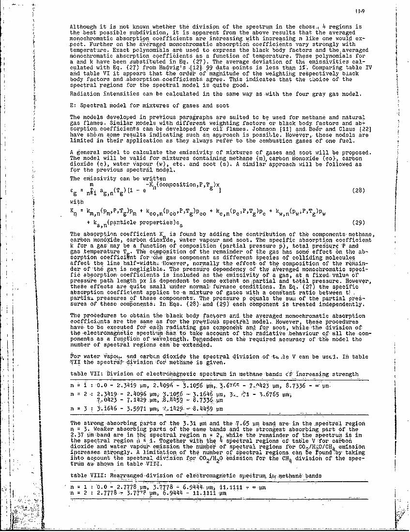
Although it is not known whether the division of the spectrum in the chose,, 4 regions isthe-best possible subdivision, it is apparent from the above results that the averagedmonochromatic absorption coefficients are increasing with increasinig n like one would ex-pect. Further on the irraged monochromatic absorption coefficients vary strongly withtemDerature. Exact polynomials are used to express the black body factors and theaveraged

9monochromatic abscrption coefficients as a function of temperature. These polynomials fora and k have been substituted in Eq. (27). The average deviation of the emissivities cal-culated with Eq. (27) from Hadvig's ,[12] 99 data-points is less than 1%:. Comparing table IVand table VI it appears that the order of'magnitude of the weightiig respectively blackbody factors and absorption-coefficients agree. This indicates that -the .hoice of thespectral regions for the spectral model is quite good.

Radiation intensities can be calculated in the same way as -with the four gray gas model.

E: Spectral model for mixtures of gases and soot

The models developed in previous paragraphs are suited to be used for methane and naturalgas flames. Similar models with different weighting factors or black body factors and ab-sorption coefficients can be developed for oil flames. Johnson [11] and Be~r and Claus [22]have sh. n some results indicating such an approach is possible. However,- these models arelimited in their application as they always refer to the combustion gases of one fuel.

A general model to calculate the emissivity of mixtures of gases and soot will be proposed.The model will be valid for mixtures containing methane (im),carbon monoxide (co)-, carbondioxide (c), water Vapour (w), etc. and soot (s). A similar approach will be followed asfor the previous spectral model.

The emissivity can be wri ttenm -Ki (domposition,P,Tg)X]Cg = n i ag,n(Tg)[ - e (28)

with

Kn,= k (PmP,T )p + k (p -oP,T )p + ke(PcP,T )p + k (p wP,T )pn m,n m g m o,in co g -co c,n c g w,n w g w+ ks (particle properties)c s (29)s,ns

The absorption coefficient K' is found by adding the contribution of the components methane,carbon monoxide, carbon dioxide, water vapour and soot. The specific absorption coefficientk for a gas'may be a function of composition (partial pressure p), total pre urP andgas temperature T The composition of the remainder of the gas has some effect on the ab-sorption coefficignt for,6ile gas component as different pecies of colliding moleculesaffect the line half-width;. 'However, normally the effect of the composition of the r~iain-der of-the ga) is negligible. The pressure dependency of the averaged monochromatic speci-fie 3bsorption coefficients is included as the emissivity of a gas, at a fixed. value, ofpressure path length px is dependent to some extent onpartial and to)tal pressure. However,these effects are quite small under normallfurnace conditions. In Eq.(27) the specificabsorption coefficient applies to-a mixture of gases with a constant ratio between tipartia pressures of these components. The pressure p equals the suu of the partial pres-sures of these components; In, Eqs. (28). and (29) each component is treated independently.

The procedures to obtain the black body factors anid the averaged monochromatic absorptioncoefficients are the same as for the preitiou6 spectral model., However, these procedureshave- to be executed for each radiating gas component and for soot, whi-le,the division ofthe-electromagnetic spect iihihaa to take account of the'radiatiVe behaviour of, 611 the-com-ponents as a function of-wa elength. De~endent on the required Accuracy of -the model thenumber of spectral regions can be-extended.

For water Vapou, and carbcn dioxide the spectral division oft. -le V can be usc1. In table-II, the spectrd,-division for methane is given.

table VII: Division of electromagnetic spectrum in methane-bands cf increasng strength

n ' 0.0 - .3419 pm, 2.09 - - 7./423 pm, 8.7336 - - -

n = 2 -: 2.3419' - 2.4096 pm? 3.1056 -- 3.1646 pm, -3 1 - 3.6765 pm-i-7.0423 - 7.1429 pm, 8._445* 8.7336pm

n = 3 1646 - 3.5971 pm il.1429 ...8.11459 pm

The strong -absorbing ar-ts of -the 3.31 Um and the 7.65 ,pm band are in the spectral regionn 3 Weaker abs rbing parts of the samebands and the strongest absorbing part Of the2. 37 pm band are in th spectral region n = 2,, while the remainder- of the spectruin is inthe spectral region i 1.. Together with the 4 spectral regions of table V :for carbondioxide and water vapur emission the number of spectral regions fbr CO /H'O/CH4 emissionincreases srbngly. A limifation of the n'umber of spectral regions can ge round by takingihto account the'spebtral divCsion'for'CO/HH division of the spec-trum ad, shown in table -VIT1.

table VIII: Rearranged division of electromagnetic spectrum iir-methan6 bands

1, ,: = 0.0 2.7778 m - 6.9444- p-, 4!4 1 C Pm'-~~ ~j -in 2 :2.7778~-3.7177? Pm, 6_-914- .11 -

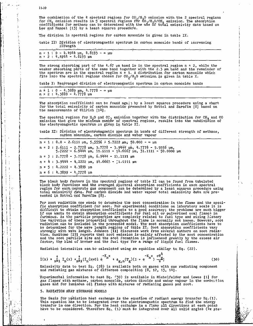
11-10

The combination of the 4 spectral regions for CO/H 0 emission with the 2 spectral regionsfor OH ' mission results in 5 spectral egions fr CO8 / O/CH emission. The absorptionc6effi ients for methane can be determined with the uge 3f t6al emissivity data: based onLee and Happel [13] by 'a least squares procediure.

'The division in spectral regions for carbon monoxide is given in table IX'.

'tabl& iXD ivigion of electromagnetic spectrum in carbon monoxide bands of increasing

n = : 0 - 4.4944 8m, .8193 - la,

n = 2 4 4944 - 4.8193 -m

The strong absorbing part of the 4.67 pm band is- in the spectral region n 2, while theweaker absorbing parts of the same band together with thie 2.3 pm.'band and the remainder ofthe spectrum are in the spectral regi'on n =' 1. A distribution -for carbon monoxide whichfits into the spectral regions chosen for C02/H20 emission, is given in table X.

table X: Rearranged divisionof electromagnetic spectrum in carbon monoxide bands

n = : 0 - 4.3889 pm, 4.7778 - pmn =2 4.3889 - 4.7778 Pm

The absorption coeffiients can be found aga i by a least squares procedure using a chartfor ,the total emissivity of carbon monoxide" ,r'esented by Hottel and Sarofim [8] based onthe measurements of Ullrich [114].

The spectral regions for H 0 and C emission together with the distribution for CH and 00emission that give the minimu numbgrof spectral regions, results into the subdivision ofthe electromagnetic spectrumas given in table XI.

table XI: Division of electiomaghetic spectrum in bands of different strength of methane,carbon mbnoxide,, carbon dioxide and water vapour

n 1 1 0.0 - 2.6111 -pm, 5,5556 - 5.7222 .pm; 50.000 - Pmn = 2 : 2.6111 - 2.7778 um, 3.778 - 3.94k4' m,, 4.7778 - 5.5556 um,

5.7222"- 6.9444 pm, 11.1111 - 1.4.6667' pm, '31-1111 - '50.0000 um

n = 3: 2.7778 - 3.777,8 tim, 6.9444 - iA.j'111 pm

n = 4 3.9444 - 4.2222 pm, 14.6667 - :1.4111 Pmn 5 :1.2222 - 4.3899 pm

n = 6 . 4.3899 - 4.778 pm

The black lody factors in the spectral'regions of table Xi can be found from tabulatedblack body functions and the averaged spectral absorption coefficients in each spectralregion for eabhh.separate gas componenb can be determined by a least squares procedure usingtotal emissiviQy ,ata. For-carbbo dioxide and water vapour total emispivity data aie pre-sented in Hottelnrd'Sarofim [8].

For soot radiation one needs to determine the soot concentration in the flame and the speci-fic absorption coefficient for soot. For experimental conditions on laboratory scale it isdifficult to obtain absorption doefficients to a good accuracy; the problems are much biggerif one 'Wants to obtain absorption coeffieients for fhiel oil or pulverized coal flamesi infurnaces. As the particle propeities are complexly related to fuel type and mixing tistorythe va-Pi'tion of these propertie4 throughout the flame is normally not known. However, soot'radiation can be included in the'presented model. The soot absorption coefficients have tobe determined for the wave length re~iens of fable XI. Soot absorption coefficients varystrongly with wave length. Johnson (11] discusses work from several authors on soot radia-tion. Kunitomo-[23] reports that soot emission is<,mainly affected, by the soot concentrationand the soot particle size and the soot formation is influenced greatly by the excess airfactori the kind of birher and the fuel type <for ao range of liquwd fuel flames.

Radiationihntensities canbd calculatedusing an equation sirUiar to, Eq; (22).

-146 -X -KX ) oT4

Wn Im(x) +nIn( 0) e + ag,n(Tg)(1, e ] (30)

Emissivity 'data to test Eq. (28) is available both on gases with one radiating ccmp~onentand radiatinZ gas mixtures of'different omposition [8,'12, 13, 14]. |

'Experimental information to test Eq; 0'30) i-s available in Michelfelder and Lowes [i] forgas flames with methane, carbonmonoxid6, carbon dioxide and water vapour in the eonbu.ticngases -ad for luminous oil flames wih mixtures of radiating gases and soot.

5. RADIATION.HEAT EXCHANGE MODELS

'The b-asis for.' diation heat exchange is the equation of radiant energy transfer Eq.(I).This equation has to, be integrated, over the electromagnetic spectrum to find the energytransfer in 6ne direction. For the heat exchange in a flame all directions at each pointhave to be considered. Therefore Eq. (1.)must be integrited over all solid angles (4T ste-

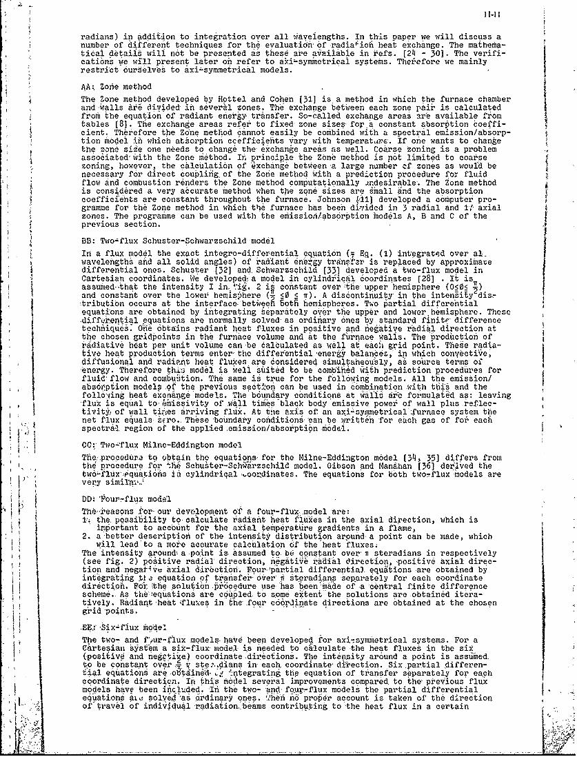
I I-I I

radians) in addition to integration over all w4avelengths. In this paper we will discuss anumber of different techniques for the evaluationi of radialiof heat exchange. The mathema-ticai details will not be presented as these are available in i efs. [24 - 30]. The verifi-cations we will present later oh refer to aci-symmetricai systems. Therefore we mainlyrestrict ourselves to axi-sym:metrical models.

AAZ Zone method {The Zone method developed by Hottel and Cohen [31] is a method in which the furnace chamberand walls are divided i several zones. The exchange between each zone pair is calculatedfrom the equation of radiant eiergy transfer. So-called exchange areas are available fromtables [8]-. The exchange areas refer to fixed zone sizes fora constant absorption coeffi-cient. Therefore the Zone method cannot easily be combined with a spectral emission/absorp-tion model in which absorption ccefficients vary with temperatare. If one wants to changethe zone size one needs to change the-exchange areas as well. Coarse zoning is a problemassociatedwith the Zone method. If, rinciple the Zne method is not limited to coarse

zoning, however, the calculation of exchange betweena large number cf zones as would benecessary for direct coupling of the Zone method with a prediction procedure for fluidflow and combustion renders the Zone method computationally a.desirable-. The Zone methodis considered a very accurate method when the zone sizes are small And the absorptioncoefficients are constant throughout the furnace. Johnson [11] developed a computer pro-gramme for the Zone method in which the furnace has been divided in 3 radial and 11' axialzones. The programme can be used with the emission/absorption models A, B and C of theprevious section.

BB: Two-flux Schuster-Schwarzschild'model

In a flux model the exact integro-differential equation (, 'Eq. (1) integrated over al-wavelengths and all solid angles) of radiant energy trunfeTr is replaced by approximaredifferential ones. Schuster [32] and, Schwarzschild [33] developed a two-flux model inCartesian coordinates. We developed a model in cylindiical coordinates [28] . It isassumed-that the intensity I in.t'i:. 2 is constant over the' upper hemisphere (05 0 )and constant over the lower hemispShere ( 5 0 < i). A discontinuity' in the intensiEy dis-tributibn occurs at the interface:'betweeR 6otfi hemispheres. Two partial differentialequations are obtained by integrating ieparately over the upper and lower hemisphere. Thesedifferential equations are normally solved as ordinary ones by standard finite' differencetechhiqueS die 6btains radiant heat fluxes in positive and Aegative radial direction atthe chosen gridpoints in the furnace Volume and at the furnace walls. The production ofradiative hdat per unit volume canbe calculated as well at eachi grid point. These radia-tive heat production terms enter, the differential energy balances, in which conlectie,diffusional and radiant heat flukes are considered simultaheu-sly, as source terms 6fenergy. Therefore th3 model is well suited to be comi'6d with prediction procedures for

fluid flow and combuiti6n. The same is true for the following models. All the emission/abs6rption models of the previous se6t*on can be used in cmbnination with this and thefoll6wiing heat excrange models. The b6undary conditions At ails are formulated as: leaving,flux is equal to-emissivity of viall times -black body 'emissive power of wall plus -rflec-tivity, of wall tik,,es arriving flux. At the axis of an axi-symmetricaltfurnace system thenet flux equals'ero._ These boundary coiditions can be writteh for each gas of for eachspectral region of the applied emission/absoptipnmiodei.

.. CC:, Two-:flux Milne-Eddington modelThwo fuedpr n to obtain the equations, for the Milne-Eddington model [34, 35] differs from

the procedure for ,I SchuSter-SchWarzschild model. Gibson and Manihan [36] derived thetwo-flux quatins 1i cylindrical,,.oordinates. The equations for both two-flux'models areIr ' very similllr

The,,reasons for- our devOlopment of a four-fluxmodel 'are:

1; the. possibility to, caiculate radiant heat ftizes in the axial direction, which isimporiant to account for the axial temperature gradients'in a flame,

2. abetter description of the intensity distribution around, a point can be made, whichWill lead'to a mo e accurate calculation of the heat fluxes.

The intensity aroundapoint is assumed to be constant over' i steradians in respectively(see fig. 2) pos itive radialdirection, 6egatiVe a i-'l direction,,positiv6 axial direc-tion and negat'vv axial directin'. Eour' partial differential equations are obtained byint6grating I l equation of trafisfei &roer' i steradians separately for each coorainatedirectioh. Fd !the solution ,procedure use-'has beenmAde 'of a 'central finite differencescheme. As the',equations are cg6pled to some extent the solutions areobtaindd itera-tively. Radiant-heat <fluxes in the-four c6rdinate directions are 6btained at the chosengrid points.

EE" Six- flux m'del

The two- and f',ur-flux models have been 'developed for axi symmetrical systems. For aCarteSian system a six-flux- model is needed to calculate -the heat fluxes in. the six(positive and negpti~e) coordinatedirections. The intensity around a point is assumed,to be constant ove- ste' dians in, each coordinate, direction. Six partial differen-'ial equations areo'taineW,, 1, ntegrating the equation of transfer separately for eachcoordinate direction. In this m6del several improvements compared- to the preVious'fluxmodels have been in'Luded. 'In the two-'an', f6,ur-flux models the partial differentialequations al solved"as 6rdinary oqes. <h@h no proper account is taken of the directionof travel of individual radiation,'beams contributing to -the heat flux in a certain

direction. In the six-filuk iaodel the heat flux in a point is a function of all the radiationbeams through this point. Even if the major'heat transfer is, in an bbliue direction reia-tive to the main coordinate, lines no special problems occur. Themost favourable finitedifference scheme canbe ch6sen dependeit On step sizes. (distances between grid points)and abs6rptiofi coefficients, Of c6urse £imila' -impovements -could be incorporated in thetwo- and fbur- flux models, but we decided to develop the next model.

- FF: CID-5 modelA iimitation in the flux models is thd assumption about the intensity distribution aroundd point. The solid angle of Ili ster.dia6s is divided into A, nw'-ber of smaller -solid anglesin, which the intensitf is constant. Then discontinuities in the intensity distributionexist at the interfaces between the smaller solid angles. However, within a flame the dis-crete radiation beams form inore- or less a continuous. pattern as a function Of the' sphericalanies'. _For the CID-5 model -we assume a continuous intensity distribution; 5 parametersare needed in-anaxi-syiun'trical system.-In ref. (2U] it is proven that the chosen distri-butioh canapproach practical intensity distributions better than is possible with the 2four'flux distributio. The solid aigie of 4n steradians is integrated separately over -steradians in each coordinate direction, namely positive ,and negative radial, axial andtangential direction. Six partial differential equations are obtained. Because of symmetrytwo of these are identical.IhtheCID-5 model many of the' improvements mentioned for thesix-flux-model have been ini6r!e9ated. Ascylindrical systems are much complexer thanCartesian systems some of othe directional effects have been -pmitted.

GG: CID-6 model

The same intensity distribution as for the CID-5 model can be used to build a radiationheat transfer model that is valid in a three-dimensional furnace where the coordinatesystem is Cartesian. In this model all the directional effects mentioned for the six-fluxmodel can be incorporated. .

6. EXPERIMENTS

Flamed from simple burner geometries are produced with natural gas, propane and fuel oil inan approximately cylindricarfuinace with an equivalent diaieter of 2.22 m and a length of6,29 m. These flames, f which a rumber combuit throughout the leigth of the -furnace?produce steep axial and radial temnperature and concentration gradients, which shouldstrongly test any radiation model. Two of the gas flames investigated will be used for theverification of the radiati6h m6dls. In fig. 6 the flame shapes of both flames are shown.The first flame is a jet flame with a lengthirof approximately 4.3 m. In this flame the gastemperatures vary between 350 K and 1600 K with severar minima-and maxima in axial andradial direction. As well steep, concentration gradients are produced. The second flame isa short bulbous flame, almost completely burnt out within 0.5 m from the burner tip,. For'this flame the gas temperatures vary between 1000 K and 1800 K. The Steepest gradients ingas temperature and- concentrations occur close t6 the burner. The thermal input of bothflames 'is about 3 MW.

Measurements of the-heat flux to 17 cooling loops are taken for a large number of flames.In addition for each of the flames, measurements are made of hemispherical radiation fluxto thewalls, intensity of radiation, gas and wall temperature, concentration of chemicalspecies and solids, flow field, etc. The incident radiat&on flux at the furnace wall ismeasured by a hemispherical radiometer, which is traversea- t the 'urnace wall along theflame axis. The hemispherical radiometer accepts radiation from a hemisphere (2n stera-dians), while the narrow angle radiometer accepts radiation from only approximately0.000007V sterbdians. The latter instrument is traversed in stps across the flamethioughthe flame axis. The measurements of radiation intensity start with the narrow angle radio-meter'looking from a short distance at a target-of fiighemissivity. By withdrawing theradiometer from the target more flame gases are between the radiometer and the target. Atseveral positions along the length of the flame" traverses are made through the flame. Theradiation intensities are caused-by flame radi6tion when a cold target-is used and bytarget radiation in addition to flame radiation when a hot target is used. Full detailsabout the trials ad the measurements are available in refi '[I]-. In subsequent sectionsrelevant,experiment/lresults willbe pr6sented.

7. VERIFICATION OF EMISSIOI/ABSORPTION MODELS

A first test on the emission/absorpti6n-models is predictifig measured emissivities.-Infig. 7 the-results are shown; The gray gas-models (A) are ot aecurate; the dependency of-emissivity on gas temperature is not -predicted. The one clear/two gray gas, m6del (B)becomes increasingly inaccurate at pressure path lengths above 0.6 bar.m. Deviations above10%-exs! at pressure path lengths higher than 1.2 bar.m. The four gray gas m~dei (C) andthe s ctrar model (D) predict measured emissivities very accurate, -

A second test on the emission/absorption models- Is the- agreement found comparing calculatedand measured radiation intensities. The int6ni:ty calcilationd are started at the target,where the, intensity equals the black body intensity of the targeti A- stepsize x of ,0.1 mis taken, and -aft&r each c~lculatiix x=0 -n Eqs. (17) and. (22) is jaoed by the stepsi-ze. $o

- complete traverie6 Of intbnsty ark obtained -Trm the'target through the- flame -axis to the-oposite wl.Ifi.8dirbtosftmeau anpataprszr e. distanceof 2.035 m from the burner wall are show for flame I of fi . 6. In figs. 9 and 10 intensi-ty predictions are compared' withmieasurements. In fig. 11 ,distiibutinE of temperature and.partial pressures At a distance of.O 37 m from-the burner wall are shown for flame I, of

I1I'13

fig. 6. in fig. 12 intensity predictions are compared with measur6ments. -Fig. 13°showspredicted and measured iftensities for fl.me 1I at 4.25 mr from the burner wall-, where thedistributions of temperature and concentratiois are rather flat. Many more intensity pre-dictions have been madeuing models A, B, C and D [28]. The gray gas models (A) are notvery ccur'ate; they d, not-predict the correct shape of the measured intensity distribu-

tions. The one clear/two gray gas- model (B), the four graygas model>(C) and the spectralmodei (P) do -not differ mubh in accuracy. Very sever- tests on these models in regionswith steep ,emperature and concebt ati6n gradients demonstrate that deviatiohi up to 40%between-the modei predictions and the measurements can occur. The largei deviationsdevelop wlhen the predictions have progressed beyond the-flame axis, which'indicates thatabsorption of radiation.emitted-at high temperatures is not correctly predicted when theabsorption occurs at low temfperature. -With the mbdels B, T and D accurate predictions areobtained, when the temperature and concentration d'tri6utiohs are rather unifbrm.

8. VERIFICATION OF RADIATION HEAT EXCHANGE MODELS

In figs. 14 and 15 predictions of incident radiative heat flux at th wall are compared withexperimental results. The CID-5 model produces quite good results for flame I of fig. '6. Infact the same is true for the Z6ne method'and the four-flux model. It is surpri3ing thatthe inacc ,.rate gray gas models and the enw-r accurate one clear/two 'gray gaq model -producesimilar results. However, gas volume elements c6ntribute to the wall heat flux in differentways as is indicated by figs 9 and 10. For fl~n'e II of fig. 6 the predictions of wall heatfluxes are shown in fig. 15 for the Zone method ahd the four-flux model. The, larger 16via-tions between measurements andpredictions occur- over -toe first part of the fNrnace pearthe burner end. However, in this part of the rurnac- th6 intensity predictionsdeviatedas well from the measurements, so pxobabiy the deviations of fig. 15 are caucea by theemission/aosorption model applied.

As the comparisons between measurements and predictions = e rot conclusive about the accu-racy of the heat exchange models theoretical investigations hav-,been executed. A numericalsolution and an exact Bessel function solution of the two-flu Schuster-Schwarzschildequations agree. The two-flux--models, the four-flux model and the,-CID-5 model have beencompared with the Zone method for theoretical test cases for whiih the Zone method producesaccurate heat fluxes [28]. To summarize these investigations on6 can state:- two flux models'do not predict adcurate radial:heat fluxes of flames with sheep axialgradients- the four-flux model is more accurate than the two-flux:models

- the CID-5 model is more accurate than the-four-flux model'- the two-flux, four-flux and CID-5 m6dels can easily be combihed with prediction procedures

for fluid flow and,ombustion- the CID-5 model accurately predicts local radiative heat pioduction- the CID-5 model ahd-,the Zone method are of comparable accuracy, however, the Zone method

is problematic in combination with a prediction procedure for fluid flow afid combustion,ifi combination with a spectral-model f6r-emission/absorption and in flames with highabhorption coefficients.

9., CONCLUSIONS

Several emission/absorption models have been developed and verified.- The one gray gas modelsare inaccurate, while the one clear/twogray gas model is inaccurate at- higher pressurepathlengths..The four gray gas model and the spectral model predict measihred emissivitiesvery accurately. When no steep gradients in temperatures and concentrations exist, theoneclear/two gray gas. model, the four gray gas model andthe spectral model predic. measured

- radiation intensities from relativelyarge gas flames accurately. The deviations betweenmeasured and -prcdi-ted- intensities increase when the gradients become steeper, which isattributed tc less accurate prediction of absorption in low temperature regions of radia-tion emitted in high temperature regions of the flame. We recommend our spectral -fnbdel, as

Sit'is based m6re on fundamentals than the other models. A spectr'al model for mixtures ofgases and soot is proposed, which can be used for flames with any composition of radiatingcomponents.

A -number of x-adiat"on heat exchange models for cylindrical systems have been developed and-verified. qhile for Cartesian iystems models have been developed. Two-flux models do notpredict accurate radial heat fluxes for flames-with Steep axial gradients. The CID-5-model

- predicts heat fluxes quite accurately., The four-flux model is slightly less accurate. TheCID-5 model and the Zone method-are of comparable- accuracy, however, the Zone method isproblematic in cobination -with a prediction procedure for fluid flow and combustion, inc0m~anion with a spectral model for emission/absorptin and in flames with high absorp.-

,tion coefficients. The flux-and OlD-models can easily be combined with prediction proce-dures for fluid flow and Combustib. The:ID-5modei acctratelypredicts local radiativejeat production The deviatiors between neasuied and redictqd heat fluxes can be partlyascribed tbthe emIssion/absorption model applied. For Cartesian systems ka six-flux model

- and a CID-6 model areproposed, in which some definite iimprovements above the two- and- four-flux-models have been incorporated. Similar improvements have been introduced in the

- - -dID-5 m06deij.

The ihformation in thi3 paper is not only relevant with respect to furnace flames, but aswell for radiation neat 'xchange in flares, fires, buildings and the atmosphere.

-10. hEP8R NCES

1] Micheifeldr, S., -and Lowes, T.K., Report on the ii2-trials, Doe. nr. F36/a/4, I.F.R.F.,-- - - IJfidideh, 1974. " " -

>1-Iv--- - a

* - 11-14 -

(2]- Pai, B.R.,Brts H, and Michelfelder, S -, Report ont the M3-triais,. Part A: cold4heat sink. An -exuerime'tlal in~estiat~or on the 'influen-ce of operational and designiai-iabies oni heat trans-fer to the furnide hearth,Doc; nr. P36/a/6, I.F.R.F.,l'Jmuideh; 1975.

'3], bartei-ds,,H., Lowesp, T.M., Michel&ldr, S.., and Pai, B.R.,j The -predicto fhaflux distr,4ibution in furfiaees and 'iis experimental testinig, Combustion InstituteEuopean Sympiui -(ed. -FJi einbr,, h1:13 88, A caemi.c" Press, Londoni 1973.

j-4] Micheilfelder-,, S. , 'Richter, W., Pai, B-.R., and' Batelds H., Uersicht Aiber Berech-kun~jsmethoden-, zur Ei'ziittJlung des Wgrine6bergangs in Brennkammein, VDI-Beiichte 246,

(5] Pai, B.R.., Michelfelder, S.,, and Spalding, 6.B,,- Prediction of furnace -hjeat transferwith 6L three-dimensi6na1 ipathemfatical mfodel, Int.3'.H-eat Mass Tiansfer,,21 5 :-580;i)78.

[6] Lowes, T.M. , and, Heap, M.P.. Emhissiorn/atte-nhuatioa c',,oeffi~ients of luminous iradiation,Second Mebr oneec' I.F.R.F., -JiJimuiden, 1-1

(-jViskantai R., jdaietransfbr and interaction of convection with radiation heattranfer, Advanees in li~at Transfer (eds. Irvine, T.F. and Hartniett, J.P'3 17-252Acadeiric Presg, New -York- 1066. -M~a-il e bk 97

r681 H"te H.,d;, aid-Qarofim, AF., Radiative Transfer, MdrWHlNe okI9T(91 Pen~rS.S., Quantitative-Molecular- Spectroscopy and Gasemissiviti~s, Addison-Wesley,

--Readilng, Mass,;,. '1959'.(1.0] Tian,-C.L;, Thierma'I radiation pr perties of gases , Advances in Heat Transfer (eds.

-HarnetJP.,andIrvneT.F-0! Vol. 5,- 253-324, Academic Press, New York, 1968.I(11] Johnison, TR. Application of the zone method,.of analysis to the calculation of h~eat

transfer from flame-, Ph.D.thiesis, Sheffield University, 1971.[12]- Hadvig-, S.,, Gas emissivity and absorptiv-it,: A thermodynamic study, J. Inst. Fuel,- 43,

129 -135i 1970,.[13] Lee,,R.H.C.,. and Happel, J., Thermal radiation of methane gS, m.adEg hm* r Fundamentals,. vol. 3, no. 2, 16Vhi762 1964l. -

[1'fl. Ull'rich, 4-, So. D. Thesis in Chemical Engineering, M.-I.T.,- Cambridge, Mass., 1953.[15] Perry, J.H., Chemical Engiheers' Handbook, McGraw-Hill,. New York, 1963.16] Sparrow, E.M., and Cess. RD., Radiation Heat Transfer, Brooks/Cole, Belmont, USA, 1970.'(17] PK ran Kuij k, R. M. .- hnd Spanj ers,i Th. H. , De overdrac'ht- van de in een vu-urhaard' van, een

stoomketel 6ntwikkeid,- warmte 6an het door de verdamperpijpen stromende koelwater, IFi'esentatiofi to "Mederlandse Vereniging voor Vlain6nderzoek-". I ,.R;F. . IJmluiden, 1975.

[18] Tobor, JAS., anid iskanta, R., Experiment and aunalysis of directional-effects on radiantK heat'transfer, Journial of 1H~at'Transfer, Trans. A.S.'M.E., 459-466, november 1972.[19] To6r, J.S.., and.Viskanta,-. A critical-examination of the validity of simplified

models for. radiant heat transfer anai'sis, Int; J. Heat Mass Transfer,, 15, 1553-1567,1972.

(20] Edwards, D.K., and Balakrishnan, A. Volume interchange factors for non-homogeneousgases, Journal of Heat Transfer, Tras. of the A.S.,M.E., 181-188,, may 1972.

(21] Siegel, R., and Howell, .,R., Thermal Radiation Heat Transfer, Vols. I,. 71 and III,N. '.. Washington,, DX., 1971%luminous flamesi.J3. Inst . Fuel, 35, 437"M4, 1962.- ,maueeti

[23] Kunitomo, T., Luminous flame emission- under prsueup ,to 20-atm. Heat Transferin Flames (eds. Afgan, N'.H., and Be6r$ JM.), 18, 271-281, Scripta Book,.Company,Washington, D.C.,. 1974.

[24] Michelfelder, S., -Bartelds, H., Lowes, T.M., aiid-Pai, B.R., Berechnung des Wlirme-flusses und der Temoera',urverteilung in Verbreninungskammerh,. Brennst.-Wirme-'Kraft,26, 1,,. 5-13, 197,4. I

[25] Lowes', T.M., Bartelds, H., 'Heap, M.P., Michelfelder,,S., and Pai, B.R., Predictionof-radiant heat flux distributi6n, Heat Transfer in:F-l ames -(eds. Afgani N.j-., and

(2]B 61, J .M.), 10,,179-190, Scripta Book Company, Washington, D:C., a9M4[2]Brtd, H.'Zranoe-dimensi6nal -fur-naoe models, sd teir1 imitations, Course

on perorman ,predicti6n'of fuirnaces and 'combustion chambers,- Ijointly gjvnb hInternational Flame Research.Fbundatiop, *IJmuideri', -nd. Imperial College,- London, at

(7-Noordwijkerhout, 15-16; ,- ~ BRA iiedfeec(21Bartelds,-H.,Lowes, T1M, Michelfelder,- S., and Pai .,Afntedfrnc

method for the prediction of radiation heat exchange, applicable to Various furnace[2]geometries, Proceedings of the Second-European Symposium on-dombustion, Orl6an6, 1975.(21Bartelds, H.., Radi'at ve -heat transfer' in enclosures, Progress report no. 8contract

no. 68-02-0202, Development of combustion system design oriteria for the controlof nitrogen oxide emission from heavy oil and coal flantes, Environme'-tal Protection

-Agency,-,Durhami, U.S.A.., -1975.-[29] Bartelds, H.,i Validity of radiation models, Course -on performance- prdcino

furnacesand combustioat chambers,. jointly given by the Internaiona - Flame ResearchFounidation, Ijmtideni anid-Imperial College, London,. at Noordwijkerhout, 1976.

(301ws TM;, Bartelds, H., Heao, M.P., Michelfelder, S, and Pai, B.R. , Peictionof furnace heat-tranisfer, presented at the 415th International Symposium of thei ~ Combustion.-Institute -at Tokio, 1974.

[-31] H6etdi, H.C., and Cohen, E.,., Radiant heat exchange in a- gas-filled enclosure:allofiande for -noh -unifolrmit ' of gastenperatue, A.I.Ch-tE. JournalI, 4, > !143 A958.

-432] Schuster, A., Asbrophys. 3., 213 1-2?, 1905'.

(33]- Schwarzschild, K.,,-Nachr. Akad-..Wiss-.' G~ttingen, Mat4-. - Physik. Kl. 1.;A1, 1906;(34] Milnei; E.A. in- Hand .buch der Astrophysik, G. Eberhard et al., eds., 3, 1part 1,

65-255, Springer,. Berlin, 1930.[35] Eddington, A.'S., The'internal Constitution of Stars, Dover Publ., New York, 1959..'[36] Gibson, 'M.M.,, and- Monahan, J.A., A. simple model of radiation heat tr ansfer from a

cloud of burning particles in 6 ofnd &steam.J Heat Mass Transfer., 14,-- 14i-147, 19,71.

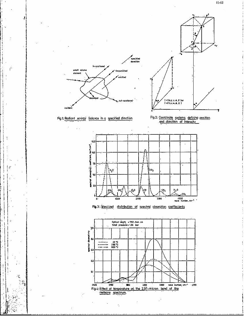
n

Specified / ndrecton/

in-scollered/ I

emitted___ F.2 Co~ Itssmsdfnr o t~e~eg~ ________ ___________

an xieto nest

.b -0- - - - - - - - - - - -

0"'0

~I I

7.5- - ... A.

, 0I 2000O 0 0 ~ 05.0nubr~m

L 1 11 1111 20 3040wae2utrCm

Fi.3,ieaied ditrbtin3f ctl bCr66lin5Cffeiet

Op 3--------------------------m1'~a - ier 1-4 aOA/

22 IC

350 30 30 10 30 w196,-Ci m9 -40

Fig.~~~56 Efeto eICeoeo h .7-irnIido hQ3~n Fpctum

) 7 ~ --~Q2

11-16

A o Roo.

i

09.0

010* A *,noPi5 mod_7

60 steel modSl C2

98% i 000000 i

0?t 1 0

Roel

to 3O 10 D 9 0 0 1102000

C~t2000K

9000

00 30

000 0MrI l

0 2 04 0 ' 0 6 0o to 1216 1

,Fig 7 Gmissv t ott axoalbdstn c of m3! on e

1400

11-17

Rlame I IFlame Ii i Experimens hot target' a Expermenls hot tragel

30 B~nx Expirim~nls cold target E5wait' To'r3. 30 wal ,r x ExPeriments cold torget

E target 18 m 'target i.8i-oe'ci Dm-fdlA XS 2.( 02

*00

200

0 0 o 0 0

0

xO:2

10 0

2800 Flam

I

AKa. dIlne 7I 02o 010.810rdildsacm 1. , 0-0 6 08 11 radia ditane.2 1.8 2.

150 x xpeimntscolntage

0 1800 F ode~ 11

/ a- 176 00xeiet o oe0/1100 40 C _I..T 004

0.0 l00~ x-xiiet odtre

C01 %1.0 T 00

008X EMo

e

04060

001.0 . 2

~000

0.26 Of 06 0 10 1goo~1. 80 0 1. 0 , 0 12 i. 2 8

Fiil'Rrtalpesurs ndte~irluesat Fi.2Pedcton~ j1ej. raerean oxa sn la/ m a teuto014aceo 0-oiuato

4 ajj 210-

I 14

*Experimentsl~~lamCID - l2 C15 model+Aida ditane &Gray medium K .2

a Experiments hont target n-IO a0 deawa~wm Crg-

C % 10'TIO43 K'** ii

25----

0 1 2 3 axoial distanice,rim, 6'

R1-99 tDeioSVN CIC)-5 model 4iith experi-

x ExiperimentsI one clear #two gray media

axi LO m ax

'tre I'l m'7.x. I

0 1 1-0 02 4 .6''W A2 -1A 16 1.'2,(Wa ilac~,s

11-i9

DISCUSSION

C.H.Priddin, UKYou mentioned briefly the Zone type method, but dismissed it because of the difficulty in combining it with afinite-difference code. There are conditions where radition can-be "decoupled!' from the flow, And compatibiiityJisthen no problem. Wbuld4ydu redofmend the use 6f Zofie methods in this situation?

Author's Reply

The following problem areas can-be mentioned with respect to-the Zone-miethod:-,coupling with finite differeiiceprocedure causes difficul ties- notvell suited for complex fuaide geometries-,for high absorption coefficients as occur in practical flames very small zone sizes are needed- for flames with temperature gradientsOsail isothermal,z6nes are needed- wheha large number of small zones is used computer time and st6r ge willbehigh

not flexible" when zone siids 6r6 to be changed- when absorption coefficients vary over furnace volume exchange areas cannot be deterniined'accurately; this

-makes the Zone-method lesssuited'for flames witti:soct, for flames with concentration gradients and in combina-tion with spectral emissioi/absorp'iion model for flames withtemperature gradients.

If the above mentioned problem areas do notexist the Zone method can be recommended. the Zone methodproduces accurate heat fluxes for certain well defined theoretical test cases. Then the Zone method can be used as a

standard'for the flux and CID models.

However, if the problem areas do,exist-I would recommend to consider radiation heat exchange models of the finitedifference, type. But then one has to take advantage of the full capacities of the latter models, which in practice isoften fieglected.

A.K.Varit'; USIn turbulent flames there-are significant interactions between the radiation emission and absorption and theturbulent fluctuations of temperatures and species.

Have you considered taking these effects into account?

Author's Reply

The differences between measurements and predictions of intensities have beeninvestigated& One of the possiblereasons for the differences are temperature and concentration fluctuation effects. Temperature and concentrationboth affect emission (e a T4), but as the effect of temperature and concentrationon emissivity e is small compared

-)4t0.thtceffect of temperature on , , temperature is the most-important parameter for the emission. When-tempera-ture r;ses emissivity falls down which Will reduce theeffects-of fluctuations on emission.

We assumed that the temperature at a poiiton-airaverse varies between the minimum and maximum measuredtemperature on that traverse. A stepwise variation from a maximum value Via the average value to a minimum valueis used in such a way, that the temperature is 25% of the time,on the maximum value, 50% of the time on the averagevalue and 25% of the time on the minimum value. The ratio uitween (T4 ) average and (Tavera e)4 has beencalculated'for all the traverses. One Vould expect the above strong temperature fluctuations only in the regions ofsteep tefiperaturegradients in axial and radii- -ire-- tion. Only on a small part:of the measured traverses the emissionwill increase significantly. Thie-predicted intensitis can be a few percent higher if-tempeature fluctuations are takeninto account. Fluctuations do not explain the'larger deviations between measurements and predictions of intensity.As well fluctuations do not-explain the'systematic behaviour of these deviations; measurements are below the pre-dictions at the axis of the flame while at the wall the measurements are far above the predictions.

iJ.B.Michel, Ne

Can CID type model predict the spectral distributionof radiative intensity and if ,yes, do you envisage comparisonswith measvredspectral data?

AjFthb;' ReplyIn principle the spectral enission/absorption model can predict spectral intensities. However the-absorption coeffi-'ients have been determined using measured totalfiitegrated over t1yspectrum) emissivity data. With go- noughspecttlinforniation-thespectralmodel can be tested and if necessary optimized.

,l ,.However the CID modeI predictheat fluxes, which are intensities integrated.with respect to solid angle. The CIDmodels can be combined with-spectral emission/a.bsorption models. These combinations can be usdto-predict

-spectral radiative heat fluxes.

We envisage comparisons with measured spectral data only when enough (financial) interest exists.

.II : ' .. . ..

11-20

F.C;LockW66d,-UKIn our work with 'Air Liquide, France,, on oxygen efiiiched flames we have fouiid that the existing grey plus cleargas torrelationis for the absorption coefficient are riot satisfactory at the very hgi~prtrseeprec.D

you know of acorrelatibn~Valid up to; say-28OOIK?I

The ,weighting factors and~the absorption.doeficienits for theone clear/two grey gas model and the four grey gasmodeihave been deitmiedusing ineasured'total 6nigsivty~dita (as given in literature)-for the tmper i -- ran&fron-I1 000 to-2000' K. -For thiespectraln'iiodel-tieblack-body factors'are~based on black-body functions. Theabsorption coficienits'are basdd-agaiii on measured, total, emissivitY data.

'Some weighting factors of the one cleai/tWo grey, gas model and-thefour grey gas model go-negative at-2800 K,

which isfi' ,iysically,'unrealk'.tic. 'Th erefore-the constants of Table 11, and IlI would need to be adjusted for-higher

For the spectral mfodel~thes ,problenis do not ,exist. The'black bodly factois are always positive. As a first approxi-maio te nfrmtin nTibe Icould 4~ue o~luae emisiite a?80k. A'better solution is to extend

Table-VI to, say, 2200, 2400, 2600 and 2800'K.I The black body factors and absorption coefficients can then-be expressed in polynomials in a similar way~ds in. thepaper.

ASSESSMENT OF AN APPROACH TOTHEICALCULATION, OF THE FLOW. PROPERTIES

-~ ~ OFSPRkY4AF Eby

Y.E1 Banhiwk and J.H. Whitelaw4echadicii -Eniieerini Department, Pluid Secticn,

Imperial Colle6ge of 'Science and, Tc'hnology, LOND)ON,?'U.K.

A method for the calculation of the l16cal'pr6rties of -spray, flames is, descritiedbriefly and its ckpabilities and,' limitations appraised "by, compaiing- calculif ed'results'with measurements. ',,The method.S-blves- elliptic differential equatiori.- repreuetn hconserv'ation of massi, momentum, enthap n pce cnetaii'infnt ifrnform. In addition,, Lagrangian. equations for the'droplet motion and thermal balance are

4solved for finito ranges 'of di6plet size A two-equation turbulence mode2.j a combustionmodel, based on mean n ~as-fraction, -equations for f uel and oxidant and a' fou1r-f lux radiationmodel are used. 'The droplet 'model assum'es' thit the evaporiating- droplets act 'a's distri-butiad point -s6urdes of fuel-,Vipour. The meriti 'of the -method are quantiied by doM~afis6nwith measuie6meits'dbtaRid' for' three difft T-enit spray flame ge6metries'. 'The assumption ofrepiesdatiiig the spray by a 'finite number,of size ranges has been Ialto examined, in- thepresent -work 'and the'result iiidicate that th e -Impq Irti.ce of this number Is'related'to theb pray type and the aerodynamic f~itures of the flow cdlose to the spray.

NOMENCLATURE

Cp specific~heat und6r~icbniant'pressure ,(J/kg0 K)i stoichiometric oxjjien i~equiremptsk turbulent ' infetic energy ( m2 is)Kf thermal 'conductivityjjof gases' (j/mOK~kg)L, fuel latent heat 0! 'japorizat'ion (J/kg)

Enf fuel mass fraction~

'fax- -oxygen 'mas6-fraction.ii the minimium value of and'iii I

%in - fu .ox/mpmask of droplet (kg)

T temperature (O ),TA fuel saturation temperature (K

Up, i' droplet 6dit' ii ' the 'i-direction (in/a)

P viscosity (kg/m~s tubAet kiicetip density ( kg/m )a ktefan-Boltzman constajit

C dissipation rate', of theL tubinkhtcenorgy

f gas phase

eff effective (including the effects of turbulence)

1. ' INTRODUCTION

-in relerence 1, the-'authors described -a-method for the 'calculation of the flow proper-

rison with' the measurements of reference,2, obtained with a hollow-coiie-spriy, and it wasconcluded -that the number of size,'ranges, was' of little "importance. In -addition,* di.scre-

'H pancies of more than 4060K were observed -in tein;'eriature, and were -attributed to unirtaintf6sin initial conditions aid in the turbulencee,modjl. The presenit paerprts calculated'results obtained with an improved' version -of the method 'and makes oprsn ihma~e'1 ~~meiixs 'obtained with -both 'hollow-cone sprays a'nd -twin-4l' s a omrs n ih maueiiThe calculat64 aa mdusoftetwo-equation turbulence model but, on this:

occsio', th -cmbutio model has been changed from that of :iefekence 1,, which was appro,'priate-dnly to diffusion flae6s, io. that of reference 3 whiich cafiiac.omodatb di'fusioi',p~emi~ y ad'bt ar ful -e flaes albeit with 'the, limitations'imppo'e, by, -sox'rce' 'termsdependent upon mean massr 'fiactio Ins Iof 'fuel afid:,oxidant. "In 'Iddition, ''ad athough of seco'n-

darimortnc' to gas turbinie conditio'i crule o uxu -radiation mdlhsbe

incorporated. The influence of the -location. of the,' -gid, nodes" neces sary in- the finite-'I difference pi-ocedurej has been investigated an u1es~ta he reiults- pies7inted hereii- " n i'ial afctd by" numerical features.

'T he-purpose -of the pr~sent. work i.s to 'allow an appraisal of- the'-calculation methodlon arlei rage of fuel 'conidJ.'tions and' gbometries thin those of'refe'rence l.' The crlcu-ltstis, as restricted to Situations withk couiparativel small or zero preheat and theItes is as a re'sult, mire- seveme than' required in practice.K

122

The itemainder of the-paper 4s presented in three sections., The foll6wink sectionprovi'des-, a brief statement of the equiCtibfii s6lved and, the louciry conditions dsed;the turbulience-, combustion, dkbpldt dfid- iadiaiion_ 6dbls are described briesly andassumptions indicated; the nu~meical ikhe'e '.i6ed to' solve the equatioiI6 is refei'enc~dandi tests of -the -ififluefid. of grid locations described. -The three test cases are des-

&riedinth spartetatsofseio 3adcrespond io the measurements of refer-ences 4 , 5 afid-,6;, the results and corresponding disciissiin are presented in these threesiubsectionis. The pa ?r e'Iids- with 'brief concluding' i~rn~rIs.

2. CALCULATION METHOD

momntu,detribul iwefene 1 dissi jt equations retresenting conserviation o1 mass,momntm, uruL.cee'ne"r~"'y',,disat ion iate', (enthalpy and Mean, -species concentrations

ca ill be wttnin thed formfi"'"a a 1 'w l a a l

('0) +i V CP r d ,+'

This presuin6s that the mean, flow. is. tw-7dimensional, axKisyrmetric h.nd that turbulcihtdif fusion 'an be -rep resented by gradienit assumptions and.'ek~hngcofiets .'h

sorerin ,,3, represents the generatio6n 'or 'destruction of he dependent variable, 4,, by sprocesses concerned only With the gas phase6, anda Sd, the generation or--destru'ctibni due to,the fuel droplets. Iflhe, .eaiation-j with thie'boundary conditions and assumptions,, described in'the following -§ubdeci6AW' 'has 'uvi solved by 'the finite-differ',ence procedure,'descrlbedin 'references 8 anIiid 9.

Boundary Conditions

The elliptic niture- of 'the differentiAl fequatItfs req~uires that each- dependent variable,or its'gadieit, 'be -specified on all liid6 of the--s6it ion' domain. I n the present case,wall and symmetry-line values were easily 'prescribed and zero -axial gradients Iwere pres-cribed- at downstream locations where: this assumptii' did not influence the- upstreamcalculated re'sults.co itosaebsdoexeietlnfrtinwhe

Upstream flow boundarycodtosaebsdoexeietlnfrtowheavailable, and on sensible guesses where not. The use of a-sensible gu~ess Iimofiea that.its -inf luenice should 'be. tested. In--general, the flow boundir'cbnditi'is for turbulencequantities are 'of secondary imiportance an'd are estimated on-, Lhe basis 'of- a mixing-lengthhypothesis. The values of the' mean'-velocity components are mo reifmportant and specificcoments will be made when, the results, are discussed. -The initial, droplet -si ze-distribu-

V tion and injectiozi v~l6city are also important and are also discussed in'relation t6- theaicsii~ results.

The two-equation, -effective-viscosity mode: used to represent the- turbulenrce charac-teristi'cs haS been -ell document~d and represents the simplest model appropriate'to -flows *with rediz'cula-tion. Higher-order mode~s, cannot-be- justified: with the uncertain-ties i-Liduced-by the additional assumptions and particularly .the ,combustion and dropletmodels.:' Equations for the turbui~nice, energy, and' dissipation rate- are 's:Aved in the formdescribed, for exoaple, in references 1 and-9, and the effective viscosity is issuimed tohave -the form

.CD . P k

The "1constant", C , and the other four "constants"- required i-o represent aerodynamipcfeatures 11are ideni'6al to these of references I~and 9. The ex change coefficient .in themomentum, equations has, therefore, the. form-

where i the entha-lpy- equation,

whre' is ad?6 '~ffetiv6 "Prandtl" 'number with' a, value 62~ -0.9.

C6nsisteht, With- th6' effective viscosity assumption and to minimiz e computer storfge,-'and run',times, the dependent variables at "the iallare linked to those at the first grid,,

node from-th' 'all by- "wall, functions" which presumie- the -logarithmic' law of the wall -

and are "dis cussed ii- ref erences 1 iu'nd 9'.

Combustion .model 1

jt ji -assumed that liquid-fuel dr oplets act as distr'ibuited -sources of f ue] wh'ich-.

L

12-3

qevapokit&'to foim~a- tcloud of vapoiti and thatj as, a xesult, 'the -combustion- pr~ce~s can -beregide' .gaseous. Tet.spi neaprion processes are r~resefitedISy xhe droplet

j ';no'del and its influunce 6nthS trm bfheiocfunnhapy ANN' mean-spe~ibsequaticnis. The combii-s'tiLn -procegs is- represented by the, model oif reference 3 wvhi-h 'presume§ihat _the ,consumption, of fikl, -', ,s control ,led by a turbulenice-chemistry intberadtih ' i.e.

*3~~~fuk '= k ~ "min ~ k/n/

where X. ib defined as the ratiobetwe~n the local concentration of reacted fuel and thetoial fuel,, 66ncentration1 cdisequently

f u EO /(J ±) f

This. combustion model can be used in arbitrary fuelled flames but is undrob tedly -si-plis 'tic ir its lack- of direct consideration of the scalar fluctuations. It is,, however,economic 61 computer storage Iand time and, iii vie*-,of th~e additional'uncekin't sii' psdby the- drbplet model, -probably,-of acdetal prisin e ip

The in!f 3,uefice of density 1fluctuatoi', in. comfbusting flows, 1, ' impob-tant and thepresent differenftial -equations may be regar ded,-a'written in m'ss-weijhtid form, with theconsequenit ass inptibn that the turbulence model is valid' in the presence' of, these f luctua-ft.ioms. This iipliies' that the calculated results'-'should be compared iith nwass-wbightedmeasurenients and,,it is likely that the measured' concentrations are close to mass-weighted.

e -Drojtlet. modelThe-droplet-Si,,e distribution within the fuel spray is- represented by a fihi-t6 nunba-

of, size ranges. Th ,drolb-!.-4urce- teirm.9 "Sd which-'piovide the meAns for coupiling the4'droplet and ,gas fields iequii-e, f6i~iheir evalua'ii6n, tli&-detei'mination ojf , the drpopirt

location, si'ze, temp6einture and ve166i-ty within the calculation domain;i This i' an bytracking -ta6e dxioplts' iepr6sentinj di'ff erent siz e ranges throughout their 'nImovem~nt inside

I the calculation domain -and. consequently -a Lagrangian f '2me~brk is- used.-to describe thedreplet behaiWbur.

For each'droplet size6 range, the momentum balance equaiori' in the i-direction iswritten as

d Up i Di. ; Ur,i Z CDRMP. dt tT

where Re is the Reynolds number'based on the~dropiet diameter,, D', and the relativeeX p1

velocit if %is the drag- coefficient andie calcaiiated~ from the correlations given inrefrene 1!' he mass transfer rate from the liquid't h~a'pae soitdwt

evaporation, is giv'en by"th-gs~hse soitdwtrefer~nce ~ fT zn~ + B) . (I ,2 ~

where BC (T - Tst)/.-lo

So that,__0,5 (3)

_____ 0-.56 Re)- zn(l + B) (3)

The droplet temperature during the jbreheatihg 'period;is determined-,by solving the thermalbalance ejuation for .a droplet moving in a gas stream:

dk -f + 056W (Tf-&T-(4dt Wp -D -t

The solution of the 'Larangian equatipns, 2', 3 and 4 providds the variation, of dropletIt velocity, dianbier and temperature i , the time domain and a droplet tracking technique

transfers thi 't6 the spac -dman Th-dipe -rce' terms are obtained -by calculatingthe loas-f ie '' fetfolt h a nd mowfitum'within 'each 'comutational cell ofthe loss o in fth drqet as ea

Radiation' modbi

The preent radiation -deisbsd6'te1u-ndlproposed',by De 'Marco-andLockwood (10) -where the directional dependenc6' of the' radint tnsity at a toint, islappobximated: by 4~ 'trun'cated Taylor- ser'ies expr ession. The exact 'integro--differentialrat io 6debcrib~ n rtd, to -1. et of- apprc~cimate -part ia, diff &rent ial, equat ions of the

'r' : -- _ - equ~ion or ai-syn~tic geometries- afiU with the assjImii

124

'&f nfi abs6rbirig' emitting non-scattering grey iimedium--in - local thermodynamic equilibrium,the: e qdtiohs 'can, be written as

4: . O I 0x 4 K (-2R - R. dT YT

x

4'a' r, a r 4 K (2R - Rx - oT)

where R and R are ,respecti-vely the total axial and radial-radiation, fluxes and. K is hebsorptfor" coefficient of the mediuh znc) has a "calculated value of O.3. The radiation,jnergy 'contribution to the s6urce term in the enthalpy equation is expressed as

S 16/9) ; K . (R +'R -2oT 4 )

Numerical features

The droplet-gas coupling is inc6rporated in ,the f.numercal procedure as Iollows. Anisothermal, droplet-free - solution of the gas field is' fiist-btained then droplet trajec-tories, size and temperature history are calculated, throu~h the droplet-field equatiOls,with known gas properties. The droplet source terms are then calculated and''fed-to tIe'finite-difference form Of equatioh 1 to obtain adjusted' vaiues for the dependefie' jaiiables.

'These ir used agair in the solution of the droplet equations. This process of s61Ving,ht gas:-fiel'd equations followed by the droplet equatio'ns is repeated un'til' all the'qut16insai sitisfied', see references 1-7.

The :present numorical :procedure is second-order' accurate except when the Reynoldsnumber of-the computational cell is greater than I2I . In such cases, an upwind-differen-cing scheme'i§ used and is more likely tb cause numericalerrors if the streamlines dofi6t orthogonally cross the finite-difference cells. Thes& 6rrors, which have the effectof introducfng ,an additional 1'false-diffusi6n" into the equations, are dependent, on themagnitude of the Reynolds ,niumber, UAxl/u, and therefore, can be minimized ,by reducing thecharacteristi" dimensi6ii of 'the' cell', Ax, at regions where the characteristic velocity,',is largely skewed,-to the ortli6gonal grfd4. , each of the s~ts of data describd' in thefollow ing seciion,l calculations were perf:i'i ed te" identify regions of highcell Reyiolds

,number -and the number of grid nodes' and "t ohii, locations were, adcordingly, imodified.Figure 1 shows a sample of the calculated, results obtained 'with different arrangements-ofthe grid nodes dand corresponds to ithe iseotrmal meafi-velocity measurements of reference 4,test case 1. The reported calculations of 'the present work were obtained with a gi dcomposed of 25 x 25 nodes which provided the best Compromise between computer storkge, timeand, accuracy. The computing time for the reported calculations varied betweenk:8 and 15minutes of CDC 6600 time 'according to the number of size ranges considered and the flowfeaitures of each tes, case.

3. PRESENTATION' AND DISCUSSION OF THE RESULTS

The present procedure hasf been applied for the predicti6n'of -the flow properties inthe three flame geometries of references 4, .5 and 6. Details of'the inlet c6fnditions,experimental data and flame geometries corresponding to (thethree test cases are givenin table land figure 2. The calculatedlresults for-erich test case were obtained with,thelpOtream boundary conditions summarized in table 2.

Test CaswAl

The experimental data of this test case, which were :obtained with a rotating cup,atomizer capable of producing a'near-monosized spray, comirised measurements of thedroplet size distribution within the sphay and the dr6plet injection velocity. Thisallowed, accurate representation of the droplet inlet conditions'and reduced the uncertjin-ties of the drop3et model to those relating to the expression used' to'-calculate' thedrople- eyaPbration rate. Supplementa'Y experimental information regarding the upstreamboundcyco'nditions of the mean-velocity'-components and 'wall-temperature distributionswere a6lso available together with detailed measurements Of' air Velocity :within -the 'combu§tor under isothermal conditions. Calculated, results were obtained for the lat:ter',as described pre ously, and were used to:,assess the 'accuracy of the present numeri"dtl

ocedure and the'turbujlence modl Th dfre., -,the 1foil6w~ing comparison with- the exermental data.l.lows the present' combustion :model ,to6,. critically appraised,.",

Figure 3 shews , the calculated and measred radial profiles of' temper'ature,.-ma~sfractions of ca'rbou 'dioxide (C0 2 )"andioxygnh ('6-) a, different axial distancgs along thecombustion chamkei. Also shown on 'the figuejfor re(ference purposes, are the correspondingmeasured profiles, of. carbon mononide. (CO) c6ncentration. The results of, figure, 3 show ,

that the general: features of the emperatur -and species 3oncentrations are correctlypredicted. Ho'wever, discrepancies in the'ietent'of chemical r'eaction and the correspondingtemperature values are clearly indicated.'in locations close to the, combustion chamberwall, the 0 concentrations are under-predictled, by approximately 5%, with, a consequentoverprediction of the temperature values,.'wh~re discrepancies of around 'l0OK can beobser"ed. The accelerated' consumption of oy (n, at this regin,, ,is attributed todeficiencies in the coupled, turbulence/qhemis'ry models and, to- a lesser extent, 'to the

oundary condition 'specifications. oIn the initial flame region, X/D <0.3, and at radiicorresponding to the ,maximum ,gradients in the .measured-temperature and species doncentra-

12-5

tions, around, R, i 60.mm the predicted' profiles of 02 and CO are seen to be slightlyshifted towards sialler radii which- indiddi e§-'. adrestifiiaion of the chemical reaction.rates. With the presumqddependence-of-the 'reaction rate-on the turbulent kinetic energyand its dissipation -rAe, this result is consistent with the und6rprediction of the centralre 4ircui'ation zone at this region which. is evident, it ffigure 1-.

The large discrepancies 4n, the temperature.values, around, 4000 K, which can be seen inthe radial profiles at X/D = 0.127a ndcO.255 and, at R < 50mm are attributed to uncertaintiesin the present combustion mode, and in particular to -the assumption- of singlq step-chemicalreaction and the neglect of intermediate species such as soot and carbon monoxide. It iscle ar that, although the 02 concentrations are, to some extent, dorrectly predicted in thisregion, the CO- c6ncentrations -are overestimated by around 30%, which can be explained byreferring to- te, high CO values, (10%) measured, ifi this zone. In effect, -and due to the

:comparatively high calorific value of CO, the- calculated heat release rates are much- higherthan -the aitual'values. At the fzr downstream regions of the flame, fol example it- X/D;'45,ne differences between the calculated .and measured temperature values decreaseg to aroundOODk and-can ba attributed, again, to deficiencies in the coupled turbulence/chemistry

models.

Test Case'.2

The calculations for tnis test case were performed, as indicated in table 2,-for 5 and-0 droplet size ranges; the, cat.culated and measured radiAl profiles of temperature and

unburned hydrocarbon (UHC) eoncentrations are shown in figure 4. The calculated profilesin the upstream p'rt 6f the flame, X/DISC < 'O.437 indicate a large overpredicti6n,of thetemperature values, by Protnd-400k, and-are qualitatively in error-especiali in theregion surrounding the intense-combustion zone,, which is indicated by the high tempera-ture values at R/DUCT 'around 0.4. The present flow-ge6metry, see figure 2, suggests'"hatthis region coincides, with the.',9iear layer separating the recirculation zone behind thedisc and the surrounding air, Itream-. It is likely that the large overprediction'of thechemical reaction rate at this region, which, is-evidended by the calculated radial profiles6f;1UHC is mainly Aue to inaccurate calculation of the mean flow and the turbulencecha'racteristics within the shear layer; The predictedhigh temperature value's in theinitial flame .region are also influenced by the uncertainties in theassumptioi of singlestep reaction-(the measurements indicated comparatively high concentrations) and in, thecalculation of the 6vapbrati6n,andspreading of the fuel spray.

The pfedicted and--Measdred temperature profiles, in the dlwnStream part of -the flame -P X/DIS: > 0.6, are-showntobe-qualitatively in, agreement although the temperatur6 values

are,:generally underestimated by around l00-2000 K. -It can also be observed-that the,predicted't iC. concentrations are well below the measured values. Apart from the relatedinfluence of thil ov6rprediction of the chemical reaction rate in the initial flame regioni.thesediscrepanci tare due maAnly toinacdscies in representing the turbulent 'transportand- eadigof the' Str am~surrounding the stabilizer disc which had'a consequentdilutioi -and cooling, oefedts on the dow'stream part 6T the flame.

The caleulated resul cs o fV.gure 4 which were obtairi d with 5 and 10 droplet sizeraft:,es in-dicate clearly that the 'hcese i, the numbei of size ranges has a relativelysmAii influence on the predicted Nro~i~es, -This small"'difference between the predictedresults is probably related to both the 6spray type and the aerodynamic features of thepresent geometry. The hollow -cone type of -dhe spray for this test case implies that mostof the droplet trajectories are conf ired-:t6 a srmal spatial volume and it is likely thatchanges in' the discretizaton- level- us6d in repreecnting the spray would have insignificantinfluence on"its overall- charateristis, including"bth- the evaporation and spreadingrates. It is also likely that the high turbulent mixieg rates in the nearrspray region of

the present .fldw geometry tend. to-diminish-he influenceo ofi any small differences in thedetails of the spray-evaporationaed' spread ng .processes associated with-the change in thenumber 6f size ranges:.

sTeitCase 3

The- reported.-calculations for'thic 'cest case were performed -using 10-,and' 20 dropletsize ranges as. indicAied-in tabl4 2. ' The calculated -and measured centre line distributionsof temperature, massfract i tns of -0, CO (measured), and co2 are shown in figure 5 and thecoriespofiding radial profiles, at aial"44-idances 6f 80mm-and 250mm are shown in figure 6.

It 1§ evident from -igure '5 that the -val'cvl-ated oxygen concentrations along, the flameFor example, -the calculated values at om6 points drop to below'half tae measured concen-trations. Related' discrepancies in the temperature and C02 Mass f~a_;tin can also beeasily detected in-ligure 5. This overpredidtion of the ch e mical fractionrateis due,in part, to inaccuracies in representing the spray evaporation rate and to-uncertaintiesin the present combustion, model. The former is clearly demonstrated by -the cqmpaiTively'better agreement betweenwthe, predicted and measured values obtained- with the higher numberof droplet size ranges. The- latter may stem from -the strong dependenceof the reactionrate term-on the turbulence- charact6ristics Of .the flow w'hich,'in turn, aresensitive tothe presumed'upstream boundary conditions. It -s also likely that, in the initiai flameregion, the combustion model may be deficient' in its lack of direct consideration of the

influence of the presence o'f high don6entratibfs of ;fuel--droplei on the calculafion of'$ the reaction rate.

it is. clear ,from the radial profiles of figure,6 that the iW rease in, the-,number ofdroplet size ranges (from 10 to 20), has led to. a be t 6i Jreijes .ntation, of the falame

4j , ___

spreading rate and ,to a decrease in, the -disdrepancies between the calculation and measure-mentse For example1 the 1tbations-of th t~mpera. ure maxima are shifted radialiy, outwardtO'boincide approximately?, with-'the measured locations. This is mainly due to theincreased ' accuracy in calculating the evaporation and:spreading rates of, the, fuel spray,

'as aresult of the 'reduced degree -of discretiZation associated with the-hiiher number ofsize ranges. The larger, influence of the number -of. size ranges observed in this case isrelated to, the spray type and the comparatively low tdrbulent mixing rates of the, presentflow geometry where-an increase in the relative importance of the fuel spray characteris-ticsl-in controlling ,the 6ombustio-prdcess 'is anticipated '.

The comparison betweefi the experimental and, piedicted results for this' case, and forthe preceding two-,cases, °is undoubtedly, subjedt 'to the expei'imental ,uncert'ainties associa-ted;with bacb, technique. Although as.essment of these uncertainties is difficult, it is.6xpected, that the accuracy of temperature measurements will, in general, be better-than 10%

and that of the onfintratiorii measuremenits-will,, at the best, be in. the range of +15%.

4,, -CONCLUDING.REMARKS,

The present procedure has been applied for the cal'culatiofi of the flow properties in

three different spray flame geometries and the coihparis6nwith the corresponding experimen-tal data indicated that the general features' of'-the flow fields are correctly' predicted.The magiitude of the disciepancies between the experimental and predicted results and therelative importance of the sources of uncertainties in'the ,modelling assumptions was foundto vary according-to the flame giometry, considered. For example, the results of test case1 showed discrepancies in the teihperE-turt_ -and oxygen concentrations of between 100 and4000 K an~d 1 and 5 0 % re~petively wh;ichi we malk'iy' inf(luenced by the delficiencies inthe coupled turbulece/cmbu~tion models. The uncertaintiet in the droplet model, however,relating to the calculation of the spray evaporitiofi and-sprdaiung rites were, however, If6und to contribute significantly to the observed discrepancies in the -es'lts of testcase 3.

The second and third 'test cases of the previous seution -corresponded to significantlydifferent spray and flow geometries and therefore,,,Pllowed the influence of the number ofsize ranges assumed within the droplet modal to be examined over a wider range of sprayflames than those of reference 1i In agreement with the conclusion of reference 1, thecalculated results of test case 2 indicated a small influence of the uumber of size rangeson the predicted'profiles. On the other hand, the results,of test case 3 d6monstratedc~learly-the importance of, thIs-numbei; ExaminatJon ofX both the sproyehlaracteris ties andthe-aerodynamic flow Ieafures, of the present i6- cases and- those relating to the test case

of reference'- suggests that the influence will -be small for sprays where the majority ofdroplets are confined to a small spatial volam i (for oxamplb, hollow-cone sprays) and forflow c'hditions where a high degree of turbulent mixing exists in the near-spray region.

-ACKNOWLEDGEMENTS

The authors gratefully acknowledgi finafcial support from-the Ministry of Defence(Procurement Executive)'aid helpful advice from colleagues in the Fluids Sectio'- ofImperial College -afid at the National Ga& Turbine Egtablishment.

REFERENCES

1. Y. El Banhawy and J:U. Whitelaw. The calculation of the flow propertiep of a confined, kerbsinb-spray flame, AIAA papei 79-7020, 1979,

2. K.H. Khalil, F.M. El Mahallawy and H.A. Moneib. Effect of combustion air swirl on theflow pattern in a cylindielal oil-fired furnace., 16th Sift. (Int.) on combustion,The Combustion Institute, 136-143, 197-7,

3. BF. Magnussefi, B.11. Hjertager, J'. Olsen and D. Bha-luri. -Effects of turbulent- structure and local concentrations on soot formation and combustion in C21 2H diffusion

f-laies. 17th. Symp. (-Int.) 0hn, Combustion, 1978.

4. Y. El Banhay Unpublfslhed work.'

-5. H. Tuttle, R.A. Shisler and A.M. Mellor. Investigation of liquid fuelled turbulent..diffusion -lamos. 'Comb. S6i.. and Tech. 14, 229 #3.

6. A.C,,Styles and; N.A. Chigier . Combustion of air blast atomiz'd spray flames. 16th,Symp. (Int.) -Combustion, The Cbfnbustion Ingtitut-, 619-& O, 1977; . .

7. Y. El Banhawy The calculation-of the flovwproperties of a confined kerogine-spray'flame. Imperial College, Mech. Eng.-Dept. ReportTFS/78/28.,,-

8. '..D. Gosman and W.M. Puni. Lecture notes- for 1, Course entitled; "'0I culation ofrecirdulaeing flows" impii al-College, Mesh. Eng. Dept., 1973.

9'. A.D, Go.maf, R.E. Khalil anid J.H. Whitelaw. The calculation of two-dimensighal turbu-

lent recirculating flQws. Turbulent shear flows, I., Ed .-by F Durst, B.E. Launder,, ;F.W. 8 hmidt ad _.H. Whitela: 237i 9,7,; sp'ringerlVerlag

10. A.d. De-'Marco andF.C. Loc1jwpod. A-new flukmodel fQr the calculation of radiation.in furnaces. Italia,,FlamdDays, la rivista dei-ComhstibiU, 29, 184, 1975.VJ W

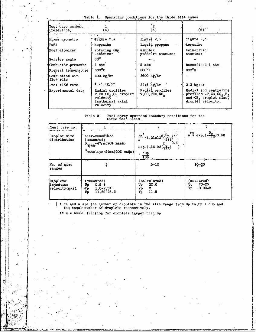
1 2-7

'U Ab 1.. Operatifig-conditionis f6r thI three t6'st cases

Test .case number.. 1 '(ieference)' (4) (5) -,(6)

Flam& geometry ';ffure ,2,a figyi6 2,b figure 2,d

FU6l peoieliud ropane -kerosihe

Fulraomzi otitin'g cup simplie* twin-fluid-at6iiizer rd6s .re atomizer atomizer

Swirier 'angle 60-Cbmhbust6r pressuke 1 atm '5 atm, unconfin~ed -1 atm.Preheat t6 peratur6 3009K 5o60K ' 3000K

'Combustionf air, '20A/r36kgh'flow 'ite'rae0k/r30kgh-~Fuel f16W rae4.75. kg/hr -22.6 kg/hir 2.3',kg/hr

Experimental data Radial profiles Radial profiles -Radial and centreline'T,CO CO0- droplet "'T,C0,UHC ,NO ~ profiles, a-T'XOCO 0 H2

Isothermal axial adoCH -drolety-zvelocity',rpe eoiy

Table 2,. Fuel spray upstreamn' boundary conditions for the

three test cases.

Z~est case no. 1'2 3

Droplet size. nermnszd . dn 4.21xl06 D exp.-)06distribution (measured) i

=47jjA(70%mads) 'D 0.4Pmean' exp.(":l698(+) )Dsatelite=24m(3%ma66)'.dp

No. of size ' 5-10 10-20ranges,

Droplets' (measured) ' (calculated) (measured)injection Up 0,9-8 Up 20.0 UP 20-25velocity(m/.4) i 1.0-2.34' Vp 2*p 03-

Wp 11.69-25.3' Wp 11.5

IL '' *dn and n are the number of dro~lets in the size range from Dp toDp + dDp andthe total' number 61 droplets respectively.

* mas r friction for droplets larger than DP

10,

' 8'~

44 4

8 60 4 20-- 80 60 20 -

-2 A

aExop' data,, ref. 4' rid 30 x 30

z 4 Figure 1. Experimfental andPredicted, radial profilesof axial: iean velodit'(is~hi'l)> far-Idifferentegrid arrangements.

-2 AAt

AA

()TEST CASE3 (A ETPAE

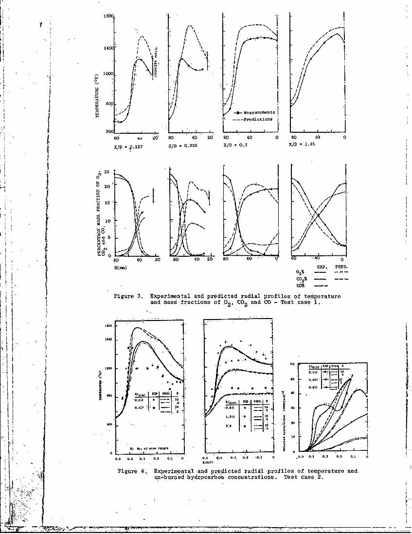
180 / .'I ' ./ -

I", I. '

146C~II

I.1 .1- I, . I

I

0 4( I 'I I

La 600

~ -- *- Meast rurents

--- Predictions

2001a

80 . .' 80 40 20' 80 40 0' 80 40 0

X/D .,, .127 X/D- 0.255 X/D - O.7 X/D -1.45

25.-

0 2

2'24' F1 " I' I

5, -

< 10

80' 40 '2 80, 40 20 so 40 .. O4

R(M) EXP, PRED

02%2

ICO%

""Figure 3. Experimentaland predicted radial profiles of temperature• and mass, friactions of ,02, C02. and CO -Test case 1.

- . ., 5' . - - ,o ."

R.,00. IE i I I IXP P-

• l~~~igure 3. E'.xperimental .and predicted rdial ,profiles of tejpez'ature-ad•,, " an-s'bur y dr ofbo' co 2 tad'ons. Test case 1.

1.3

,Disc. £XP S-0.4:7 0.1131 '

1,312 & 10 '

0 - 5

0.5 0.4 .0.3 .0.2 0.1 0 0.5 P,4 0.3 0.2 ~0.1 0.0.5 0.4 0.3 0.2 0.1 0

Figure 4', Experim~ental and predicted radial profiles of temperature -and.11ik' nburned hydrocarbon concLentrafions.- Test case 2.

7777R

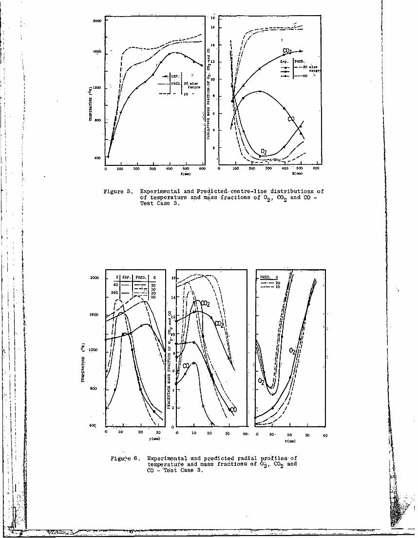
2000 1

12 Ey. PRED.... -20 size

010 ran"e

,.-PRED. 20,size ,

P.0-, 24

400-

Tes Cas 3

120- 20kle

10 10

260- 20 If~\

4 'Va1n) I

160 X X.,PtD 12 PRE. 8

1/1

1 20 20 0 0 2 0 4~ 0 10 2 20 4

4600__ _ _

121

DISCUSSION

A.M.Mellor, USI believe that test case 2 shows little dependence on the number of size ranges used to model the spiay for tworeasons:

(1) The liquid propane isthought to flash evaporate when injected into the combustor;

(2) The flame you have modelled is thought to be controlled by the mixing of fuel vapor with air, that is, evapora-tion is rapid compared to this mixing (see Paper 24,.this Symposium, Figures 10 and 11, and Reference 48of Paper 24).

Author's ReplyThe calculated results support Dr Mellor's interpretation and confirm that, of the three sets of datatested, onlythese trom the twin fluid atomiser with its polydispersed solid spray, require a large number of size ranges. It islikely that, except at idle conditions, droplet considerations are of secondary importance for gas-tiurbinie calculations.

J.Swithenbank, UK(1) Although it may be justifiable in some cases to use only -a few droplet size ranges in evaporation computations,

our studies' have shown that for a typical pressure jet atomizer we obtained virtually the same results with20 and 40 increments and significant differences with the size ranges. Vwe therefore feel that at least. 10 sizeranges areneeded in such systems.

(2) We should try to elevate the choice of gridsize from the state of at. 'art' to a,'sciencf,. Perhaps the turbulencelength scale can be used to iteratively. optimize the g rid.

I welcome your comments on these points.

i. Vincent, M.W. Droplet Evaporation in Combustors, Ph. D. Thesis, SheffieldUniversity 1976.

Author's Reply(1) The results I presented have related to threesprays and show significant influence of the number of droplet,

sizeranges only for the solid spray. The more practical hollow-cone arrangeinents-clearly did not require more

than 5 size ranges. The previous comparisons, presented at the 4th Symposium on Air Breathing EngineSymposium support thisyiew. This is not to say that sprays with different characteristics will allow differentconclusions. However, it seems likely that theneed to better represent the chemistry by, for example, a two-stage reaction will result in discrepancies which are more important than these introduced by the considerationof asmall number of size ranges. h1e incorporation of this better chemistry, with appropriate influence ofturbulence, may require considerable effort:

(2) 1 agree with the view that the location of grid nodes requires skill and that a-more systematic and automaticprocedure is desirable. An important question is to identify good criteria for this choice. We have found, insome flows, that the consideration of the static pressure distribution, and the location of nodes with concentra-tions'linked to the static-pressure gradients, gives good results. But the criteria may be Preferable in differentflows, and numerical experiments are necessary to identify them.

Atthe same-time, we need research with the magnitude of numerical diffusion effects as a function of finite-difference scheme and flow. This'is-at least as importart as automatic node selectioh, although the two may simply-be coupled. In many practical flows, with realistic numbers offnodes, numericaldiffusion is iitroduced to retain

stability, with large but inadequately quantified effects. The effects need to be quantified andwhere necessary,avoided,-eitler by abetter distribution of grid nodes, bybetter numerical schemes or by a combination ofboth.

Vt74 ~- ----

FUNDAMENTAL CHARACTERIZATION'OF ALTERNATIVEFUEL EFFECTS.IN CONTINUOUS COMBUSTION SYSTEMS

by

R..B..Edelman, A. Turan, P. T. Harsha, and E. WongScience Applicatibos, Ific.

Combustion Dynamics-and Propulsion Technology Division20335 Ventura Blvd/Suite 423'

Woodland Hi-Us, California 91364

W. S. BlazowskiExxon, Research and Engineering Company

rGovdfnment .Research LaboratoriesP.O; Box:8

Linden, New Jersey 07036

SUMMARY

Increased interest in alternative fuels use in gas turbines has prompted questions relatedto the impact of fuel property variability on'thecombustion process. Reduced'hydrogen~content is characteristic of syncrudes, that have been identified as-probable alternate

fuel sources. An interrelated analytical and experimentalpr6gramis being condicted -inwhich chemical and aerodynamic interactions are being inrestigated in order toprovide atechnology base to ald in dealing with probiems of burning alternative fuels. One elementof this effort is devoted to characterizing the'kinetics of the oxidation of alternativefuels. This pape is concerned' principally with the problem of net soot-generation whichis aggravated by the reducedhydrogen content. The-kihetics of- the-process is being modeledusing the quasiglobalcohcept while experimentaldata is being developed primiarily from-alaboratory jet stirred combustor. Results are presented showing that ,sootemissions canbe-characterized'in terms of major species and that soot oxidation must be included in thelprediction of net soot generation., In addition,"the tedhni~ues'being,.employed for coupling.the che'mical and- aer6d namicprocesses are outlined.

INTRODUCTION

'Until recently the development of gas turbine- combustors as well as ,the -development ,f,combustion chambers for most other applications has been'based largely upon empirical:methods. While reliabli,&systems have been produced by this approach the cost is becomingProhibitive. Furthermore, time, constraints fori.the development of new systems by thisapproach-ar6 not necessarily c'ompatible_.with meeting-near term requirements,,fcr cleaner

burning andmore efficient systems. Not only do the near term hieeds blunt purely empiricalapproaches but we are in a critical period where thedevelopmentof new technology basesmust be initiated and sustained, to meet the'long term requirements dictated by the in-creasingly changing fuel availability picture,. Although economics and supply are-primarilyresponsible for this recent'interest in new fvuel'souroes, projections of available'world,wide petroleum-res6urces also indicate thenecessity for seeking non-petroleumbased, fuels.

Fuel variability has not 1een a factor commonly accounted for in empirically based designprocedures. Because of the uncertainty ih, future fuels-as well as the-need to use lessconventional petroleum based- fuels, the requirement to develop fuel flexible systems is

I I well established, The-design- of fuel flexible combustors that burn cleanly and efficientlyrequires a more precise- ndersttflding-of the mechanishs that contr6l flame structure thanhas-been needed in the-past.

The practidhi goal in urnderstanding the combustion process is to relate the parameters inthe control of the designer to the p&rformance of the system. By performance we includein ageneral, sense- combusti6n efficiency hnd 6mlssions characteristics."

- In this paper emphasis is given to-the effects of fuel properties on combustion but therelationship betWeen the fueland the aerodynamics of the gas,turbine combustion processis also addressed.- ee a ot s um

FUEL EFFECTS ON GAS TURBINE COMBUSTION:

Fuel characteristics which are most likely to, affect the design- of future gas, turbines arefuel -hydrogen content,'viscosity, volatility, nitrogen content and thermal stability,Ref. 1.

The impacts of reduced 'fuel hydrogen;,content are associated with increased rates of carbonparticle formation. Increased revels,;of darbon, particle concentrations formed in fuelrich regions of the primbary zone leadto -higher liner temperatures and higher snmoke emissions.Reduced volatility and increased viscosity affect dropletlife times and, atomization,respectivel-,. Volatility affects the- rate at which liquid fuel introduced into thecombustor can vaporize. Since important heat release processes do:not occur until gas phasereactiphstake place, a, reduction of- vblatility reduces, the time available for chemical

reaction 'within' the 6ombustioi, system. In'the aircraft engine this can result in difficultyin ground or altitude' ignitidn capability, reduced combustor -stability, increased--emissionsof carbon monoxide (CO) and, hydrocarbons (HC), and the associated loss in combustion effic-,ioncy. Moreover, carbon particle formation is- aided by the formation and-maintenance offuel-rich pockets in the hot combustion zone, Ref. 2. Low volatility, allows rich pockets to

pL

persist because of the -reduced-vaporization rate. Again, increased soot can causeadditional radiative loading-to- combustor liners.

The.desired formation of a finely dispersed spray of small fuel droplets is adverselyaffected by viscosity. Consequehtly the shortened time for gas phase combustion reactionsand prolonging of fuel-rich pockets experiencedwith low volatility can also occur with

increased viscosity. Ignition, Stability,-emissions, and smoke problems also increase forhigher-viscosity fuels.

Increased fuel bound nitrogen levels can lead to increased NO emissions. Indications arethat bound nitrogen conversion to NO 'can be mfinimized in fuef rich combustion, Ref. 3.Apparently, this-will occur if sufficient time, under fuel rich conditions i allowed for

Sdirect conversion of the bound hitrogen toN. Problems of fuel stability are aggravatedwith increased bound nitrogeh and undersibl&- levels of carbon deposit buildup in fuelmanagement systems and on combustor domponents-can odcur.

While our investigations are addressing all of these fuel related problems it has becomeapparent that to characterize netisoot generation requir a broader description of thekinetics of pyrolysis and partial oxidition.

While both carbon formation and carbon consumption processes occur in continuous combustionsystems,, the latter are very much slower. The optimum approach for preventing hardwaredistress andavoiding serious environmental consequences is to develop technology to avoidcarbon, formation while satisfying-ot ir system requirements (efficiency, gaseous emissions,hardware reliability,. etc.).

NET SOOT GENERATION

The piredominance of fundamental research ,activity has involved-laminar premixed flames.Street and Thomas' work published, ii ,955, is extremely thorough-in experimental detailand breadth of hydrdoarbons examinedi Ref. 4;,it has become the classicalIpaper inthefield. Otherpublicationsafe'Referedces 5-16. These investigations have univernallyconfirmed that soot formation is a kinetically controlled process. Equilibrium calculationsindicate that soot should no6 Ibe present at fuel-air mixture conditions where the Oxygen-to-carbon atomic ratio'(0/c) is greater than -one. That is, the general chemical equation

Cx~ ~-y + 2~XCO + X, 112should-define-a soot formation threshold. All experimental- results have shown soot formationat O/C.,substantially in excess of-unity.

Another very important premixed flame experiment conducted at the British National GasTurbine Establishment (NGTE) attempted to evaluate the effect of pressure on soot formation,-Ref. 11. All previously mentioned work with premixed flames concerned atmospheric orsub-atmospheric conditions. The combustion system employed took special precautions to avoidflashing back to upstream locations, an additional difficulty associated with the highpressure operation. In additioi to sooting limits, the amoint- of soot formed:was determinedand expressed as a "soot formation:ratio" (the percent of fuel carbon--evident as soot).The index of the soot quanity was found to increase with the cube of pressure, Very use-ful plots of pressure versus -equivalen6e ratio fr -various values of soot formation ratio-were persented. Examples are shown in Figure 1-for cyclohexane, cyclohexene,, and benzene.Gas phase -species-were also determined during this testing and it was concluded thgt H20and C02 (oxygenated compounds not predicted, by equilibrium for the system (CHl + 0xCO + JHi) are formed'in,-ubstantial quantities and deplete the system of oxggen pr or.to consump ion of all fuel. -- ..

Soot formation ih laminar diffusion flames has also-been studied, Refs. 17-20. The direct-utility of'this information for the gas'turbine combustion application has been questioned,as, the mixing rates and characteristic times,-for Chemical reaction are very much, differentthanthose in the typical-combustor. Shirmer, Ref. 21, has discussed the significantdifferendes, between'such -experiments and the actual coinbustibiiproc6ss. He is particularly-critical-of the-use of the smoke point test as an index of ,fuel tendency to ,form carbonparticulates. Turbulent diffusion flame results would appi'io be more applicabld, Ref.22., Wright, Ref. '20, ihas examined soot' formation in a diffusibri,-flame burner and._published results of soot measured when the fuel side of the flame is supplemented Withoxygen at concentrations well below O/C = 1. Surprisingly., it was found that the additionof oxygen increases" soot formation up to an pptimal rate at which the influence--abruptlyreverses and sopt suppression- is accomplished at higher 02 99nentratidns.Wright's work inyolving soot formation in the Jet stirred reactor, Refs,; 23, 24, is perhaps

Of most interest to this discussion -- it is a combustion process similar to that at whichsoot forms in -the primary zone of anactual continuous' combustion, system. As in the pi'G-viously mentioned studies, it was determined that soot forms atO/C > 1 but he strongbackmixing of the jet stirred roactor did &fiord some broadeningof the soot-free 9/Cratio. In addition to- the establishinent -of sooting limits, as determined by the colorof the flame (luminous yellow versus blue), Wright determined'the ooncentrations f soot

V formed, for some, liin itdU 6ondition of 0/C below the. 6ot lfit. 'NO analysis of this"yield" data to determine soot formation kinetics wasuhdertaken'but it is ie'6gfiied that-more such daid I might provide ithe asis-for global carbon formation-'chemicil model.

MODELS OF-SOOTFORMATION, .i

Many.studies on soot formatioij have been-carried outj buk few lead .-Io quantitative

-- ~17

preeict ions of soot-productioi, and there is little agreement as to the details of the-mechanis.n. Nevertheless, there seems to be-general agreement that the overall soot formationreactiow _is.irigg~red by hjdlrocarbron pyrolysis and involves subsequent soot nuclei formation,s6t Par'ticle, forma:tion, and, Particle growti nd coagulation. A model that treats thesein- some detail has, been, consider ed by Jensen, -Ref,. 25. Application of. the-model to a methaneflame ~his led~ toqualitative-agreemenit with experimental obsi't . -Alithough thiapproach respresents an attempt to deal with the problem at a m6chanistic level the un-certintky of intdrmediatib sp ecies,' reactions, and rates requires long term- development to pro-

~vie ~iatiatie redctons T'ser, et al., Ref . ,26, 'have'proposed amodel in which sodt

formation is'characterized', by three rate equation's. The feature of the model is that allth6 complex elementary steps associated, with pyrolysis, niuclei. f ormation and soot f orma,ionare grouped into thri,' subglo'bai 6tep's which are characterized by three separate equations.The ,model includes d first ordei~ (with respect to hydrocarbon conicentration) pyr~olysis rate,achain- braiiching and chain termination 'rate, and' a soot forma' n ae

'Pyrolysis': N-lOi3'N e -170,0OO/,RT 1_ 0

Nuclei Formation, dn N -- 2'

Soot Formation dNu (a -bN)n 3

Values of the kinetic parameters (f, g, g ,a, j) for acetylene and tolueie are available,so that the model can be evaluated throug~ comparison wi.th experimental data. Comparisonswvith data developed in this inve'stig ,atiin are p'res66nied later in t Ihis p aper. Greeves, etal., Ref. 27, developied a-model using, dieskl enigizie data obtainied'unerdhpesrsThe model, consists 61f a single,'global Arrh~nius type equation:

dS 4.68x 105 P' e' 40,0O/RT 4dt d

*here P',and are the local partial pressure of theunburnt hydrocarbon and the localequivalene ratYo, respect'ively, This type of one-step model lumps all intermediate re-actions associated with nuclei formati'6n-and' soot formation into one raite'equation, andVhe application, of the' model requAires knowledge-of the local hydrocarbon concentration

jand the unhburnt equiva'lence'i'ati6-.

Attempts to co~relate~data developed in-this investigation,.with,G;Qpve5.mode], Equation-4, are presented in this paper.

The Greeves and-Tesner models represent the'esse;niial state-of-Tthe-art of prdcticalI sootprediction methods. However, the process' requires information on certain intermediatesthat must be assumed in order to implement these',models in a strictly predictive mode. Thisinformation includes, for 6kample, the local hydrocarbon and' okygen- concentrations-as wellas the temperature. In addition, net soot generation requires not only consideration ofsoo9t formation but its-oxidation as well. These factors are included in the current model'development.'

QUASIGLOB3AL MODEL

The essential.,feature of, the quasiglobal concept is the coupiing of .a set of subklobalsteps to~'a set of detailed steps for those reaction _chains for which sufficient informationto accirateiy describe theii kinetics and medhAnisms exists. the basic qjuasiglobal model!sie8'6rib&d in Ref.' 28. In ad'dition to havinig demonstrated the ability of the quasiglobalmobdel 'to"icd~ experimental ob'servations' i't has been shown to be ideally, structured toaccount, for the variaition in fuel type , i.e. ali'~hati6 vS.. dye'ic, etc. Of particularinterest here is the'dcur~rent wxork 6n- fuel rich systems f 6 - w'hicl hi basic model i's 'being 1extendedI. 'The new model'includes the following additional subglobal finite rate react'ionsteps gi'>en below in skeleton form:

Pyrolysis: C nH mBY + ti- C xH y+ M'+ BN (M=_ thtl'd body) '

'1Paiftial Oxidation: C Hm +Z02 CO "H2 6

0C, Hy+ 02 4-6,

Soot 'F6rmation: ChH6 -t C0(s 8

WhrNrepresents the bound nitribqn. Reactiors '5' through 10 are cou~led' t6 detailed'mechanisms de scribing't6r~ at w~hhH H.Cai,,N'r oere t CO an-N

Th aeconstants frtesinbklQ )al step& aiep-?resd rmoiedArhuP r inofprduction (ox ~dupio is "gfi.by expression of the type:

C1 .: T-C~ e, p (- ,/RT) 111wher~e the constants A, a, b, 'c and E are determined, through controlled experiments. The

'7ih7__

reactions and rates associated with the detai'.ed steps ar e based upon available literatureiralues.

The quasiglobal ,model- has been uged sucessfuly,for high endri fuels, such as shelldyne-H and'Hmethylcyclbpentadiene, as well as 'fbr cohventional fuels such as Propane andJP-types. The versatility-of this apprbach-has been demofistrated by comparisions withexperimentally- determined cofibustio- characteristics-includifig ignition delay,-times forboth long chain and cydlic type hydrocarboris reacting in air. For example, Figure 2 shows-some typical results of such a comparisoh betw2en predictions and data obtained from asteady flow- reactor: Figures .3-, 4'; 5, and- 6 ,ihowv, 'comparisons of Predictions with cufrentdata: obtaiied in a ieactor' described, later. Figures 3: and 4 compare data with predictions for0- and CO-concentrations. The agreement between the predictiobs and the data is very good.Oipartlcular interest are the CO and hydrocarbon coficentrations since they both relatet6 efficiency and emissions, while the hydrocarbonconcentration relates to soot formation.Figure 5 shows the CO conzentration coinparison where -kta for three- fuel types is given;ap9arafin (isooctane), an aromatic (toluene), and an olefin (ethylene). While there aremdasueable differences amongst :the fuel types the prediction -for the CO concentration isreasonale, noting that the concentration levels are in percent. What is significant tonote is. the minimum in CO at equivalence ratios between .4 and .6 depending on the fuel.Tliis-,miiimum is reproduced-by the prediction and is associated with the approach to blow-out at the low equivalence ratios where 1ow temperatures (reduced reaction rates) enhanceincomplete combustioi ,, while at the higher equivalence ratios reaction rates increasesince temperature is increasing, and-although the system is out of equilibrium, thetendency towardequilibrium is consistent with the-water gas shift reaction tending toincrease CO (and '20). The ability of- the quasiglobal model' to predict this type of detailis relevant to the determination of 'Optimum ' operating conditions, and tO scaling to 6ther

operating conditions. Of equal importance to the CO concentration is the fuel- conversionAnd 'Figure 6 shows the hydr6carboi conentrationas i6measured and compared with-predictions.The comparison is favorable considering the low-concentration -levels of fuel existing inthe system under the particular Operating conditions. The rapid rise in the hydrocarbonconcentration corresponds to the approach to blow out and is consistent with the increasein,.CO. previously cited.

The 6xamplescited above Were used'to illustrate s6ihe of the features of the quasiglobalmodel. For the prediction of net soot 'geheration ad'ditional information related toreactions 8, 9,and 10 is required, The soot model is constructed in terms oftwo stepsreflecting the dependence of net soot generation on the simultaneous formation and oxidationof soot particles. The: soot formation irate isassumed to be-a function of: the hydrocarbon

coficehtrafi, the oxygeacioncentration and the temperature; viz.

w A R+ =A, Ta Cb C--E/RT 12SC~s ) HC 02 ' 'e1

4 where A, b a and E are constants. Theokidation' step is based upon data involving theconsumption of s6ot (and carbon-) particles: in oxidizing envirinments, fromj forexamplethe work of Leej Thring and Beer, Ref. 29, and the work ofNagle and Strickland-ConstableRefs. 30 and'31. For the Lee, Thring-and Beer model the rate of consumption per unit su:-taceArea 'is given by PO

R . =1.085 x 104 2 exp ( -9,300 ), 13R (s)

w here P is -the partial pressure of okygen ini the mixture, Reactions 12 sand 13 areombineA2.to y~eld the net rate bf soot prbduction as ~A'fin6tioh of hydrocarbon and oxygen

concentratiofis- and temperature. 'The constants A,, a, b, a-and E have been determined fromekpeimentall data ahdit is interesting to note-that net soot production is more strongly,dependei't uoh ,the Aydroairb6n conientrations that on, the temperature. It is also

f:> .important& not e , a6 will be discus6d later,. that as much- as 20-25 percent of tho sootformed daifbe 9onsumed by'oxidat-in.-

ExPERIMENTAL -METHOD

The experimental program focused on -a study of the soot formation process using the Jet-

Stirred Combustor (JSC), shown schematically in Figure 7. This device is a modificationof the-Lofigwell -Weiss reactor', Ref. 32, with hemispherical geometry. The JSC has been usedextensively in fluid'mechanic and combustiobmmodeling because combustion rates, are limited

by .chemical kinetics as opposed to transport-effedtsi A"key advantage of the JSC for the-work described here is that the strongly backmixed-nature of this-combustion process pro-vides, a simulatiowof the recirculating characteristics of'the-gas turbine primary zone-It is in this zone where mixtkureconditi'ns are sufficieuitly rich to produce 6oot. Con-

-sequently, -the-JSC' allows study of soot formation-in an, aerodynamic sit;Aation relevantto gas turbine systems. Another advantage-of the stirred coixbustor is that the reactors homogeneous in species 6ncentration as well as t..era.ure; each operating condition6sntempertre; ea oprather' condition

-is characterized by a sifgle set oftemperature and ... a dat rk 'nand- concentrreation daarther hnpoi ~fles of these parameters.' This simplifies the task s of obtaihingand-interpretating the

Details of the experimental apparatus and measurement techniques used have been reportedby Blazowski, Ref . -38.' The rheadiremen n---- ~cniq use -veben re arents include fueX' and 'air mass flow rated and fuel/airmixture injection temperature, reactor gas :samples and- reactor int6rnal and wall temperatures.Both gas-phase and particulate sampling systems are used providing data on the incipient - -

soot formation equivalence ratio afid quanititativd dati onsoot production (mg-soot/liter).

V- -

13-5

EXPERIMENTAL RESIULTS I-Detailed experiments were conducted usin& the Jet Stirred Combustor to determine the sootformation-characteristics of ethylene, a hydrocarbon thought to,:pr6dce combustion infor-mat'in representative of aliphatics, andtoluene, a condensed-ring ar6matic. 'Substantialdifferences in the behavior of these two 'hydrocarbons were-noted, and a-humber .of .otherhydrocarbons were studied to determiine whether they 'behaved 's H oras C H5CH . Finally,the soot formation characteristics of two-component fuel blen~ds anlpracticl. e~roleum ",derived fuels have been investigated.

Chard;cteristics of.Ethylene and. Toluene.

Jet Stirred combustor~experiments with-ethylene sho¢ed that COwas the major carbon-,containing, species-and'rremained at a-concentration of about twelve mole percent forall equivalence ratios tested. Total] hydrocarbons increased significantly with equivalenceJ'ratio-but CO decreased- Oxygen concintration was very low at an equivalence ratio of1.77 but steadily increased at higher equivalence ratios--an indication of poor reactednessas the mixture was further enriched. Furthe , THC concentrations were found to be verysignificant at the even below the incipient soot formati6n limit.

For toluene, CO was again found to be-the predominant species. However', a substafiti ldifference beween the data for toluene and that for ethylene Was observed: whereas withtoluene, incipient sootodcured'as hydrocarbonsbegin to "break through" under richoperating conditions,, the soot limit for ethylene, occured at conditions where hydrocarbonconcentration is high - a factor of 36 times that for tolueneIResults for thesetwo fuels, described in detail in Ref. 33, indicate significant -differencesbetween the soot formation process for ethylene and toluene:

1, Toludne soots asa much lower equivalence ratio (1.35) thanethylene, (i.'95), and the, amount of soot formed with increasingequivalence ratio beyond'the -incipient -limit is much larger.

2. In the case of ehtylene, -significant amouhts, of hydrocarbons(N3-8%,as CH ) were' present at equivalence ratios; leaner thanthe soot limft, butwith toluene'the incipient soot limitcorresponded approximately to the equivalence ratio for theinitial presence-of-lhydron~arbons, in'the, comb'ustion/products.

Sooting Characteristics (of Other Hydrocarbon Types

The obser~ationsfor ethylene and toluene indicate that there is a fundamental difference'in tie, so~t form~ation mechalnisms'.tor th~se two fuels under-the strongly backmixed conditionsof the Jet StirredCombustor. These findings lend suppoft to the'possibility of developing

,useful simplified overall chemicalkinetic models of the soot formation process (quasi-global models) based, on hydrocarbon type. In order to further develop this concept 'a largenumbi of other fuel types were screened to determine whethbr their sooting characteristicswere sL ilar to ethylene or toluene, or if they showed characteristics distincly differentfrom eithei of these fuels.

It was found that all hydrocarbons tested.,might be grouped. into three categgries-as follows:

Like C2H4 Like C6 HCH3, Unlike0214 or-CdH ,3

Hexane O-xylene l-methyl;napthaleneCyclo-hexane M-xylene

t V N-octane P-xyleneIso-Octane CumeneSl-octene Tetralin e

Cyclo6ctane DicyclopentadieneDecalin

The first group produced large amounts of exhaust hydrocarbons without sooting as did

qthylehe and in no case was significant soot observed. The second'group produced-soot atA th4 mixture ratio which corrspondeo to hydrocarbon breakthr6ugh. In all cases themeasured hydrocarbon composition was less than one percent at the incipient limi-t. Anothercommonality 'in the second group is that the amount of soot pioduced as equivalence ratiowas ifireased beyond the incipient limit'-was similar foi all the hydrocarbons. i-methyl-napthalene was sig'ificd tlydifferentoin this respect producing much higher soot quantitiesthan those in th sedond, category.

Sooting Characteristics ofFuel.Blends

Blends, of iso-octane and toluene were tested to determine the behavior ofa two-componentmixture with Group '(like-CH 4 ') and Group'2 '(like-C H CH?) lhydrodarbors. These results

areshown in'Figure 8. Mixtures with, 50 or more percent tdluene-produced soot while a'25%toluene'blend did not. Clearly, for the mixtures which did soot,, increases in the volume.Percent tdllene. esult in increased soot production at'all'equivalence ratios. With' less,toluene in th6 blend, the concentratioh of hydrocarbons at the incipient limit tended to in-crease. These r6sults 'indicate a combination of Group '-lard'2 behaviors; thus a combinationof the analytical descriptions, for toluene and is6octane might be a reasonable approadh forprediction of the sooting characteristics Of fuel blends. Anex~elldnt correlation is ob-L tained between sootconcentration and hydrogen content, Fig. 9., This is in -direct compliance

I'

with actual gas :turbihe tests, Ref. 1. The similarity between suoting characteristics in

the JSC and those in' an actual combustor is evident.

Mechafiisms ofiSoot Formation

Manymechanistic-models fo- seot formation have been-proposed. Generally, it is recognizedthat condensed ring araftic hydrocarbons can, p'oduce soot via, a different mechanism thando aliphatic hydrocarbons. A simplified,,dechanism following Graham, et &L. .Refs. 34 and35, is, as shown sdhematic'all in Fig. 10.,

Aromatic hydrocarbons can-produce soot via two mechanisms: a) condensation of the aromaticrings, into a graphite-like structure, or b) bieakup to small -hydrocarbon ragments which

-thefi -poiymerize to form large6r, hydrogen deficient molecules which e6nually 'nucleate andpr,dude soot. Based on, hisshock tube, studies of soot fbrmatin-, Graham concludes thatthe condensation route is much faster than the fragmentation/polymerization route. Further,'he has fou dthat the mechanism by which an aromatic f6rms soot ,chani es with temperature;below 1800 K the condensation path is favored while above this temperature the fragmentation/polymierization route" is fllowed.

According to this simple model, aliphatics, produce soot via the fj~gmentation/polymerizationmechanism only. As a result,, these hydrocarbons do not form the juantities of soot pro-duced by the aromatics. Indeed, duringthe fuel rich combustion of a fuel blendcomposedof aromatibs and aliphatics at, a t(,iperature -ess than 1800 K, the aromatic'hydrocarbonswoul&-produce- the major p6rtion of'soot. Combustion of the aliphatic portions of the fuelwould:influence temperature and hydrocarbon fragment concentration but-soot formation -viafragmentation/polymerizationwouldbe-minimal.' Above 1800 K, however, both the aliphaticand aromatic hydrocarbons would-produce soot via the fragmentation.-/polymerization route.

The experimental results obtained-in the present work are consistent with this model. Ithas been observed'that soot formation with the condensed-riiig aromatic fuels commenceswith the initialjrisence of hydrocaibons in the exhaust. If it is assumed that thesebreakthrough hydrocarbons maintain their aromatic character, this observation reflectsthe fast kinetics: of the ring-building or cond6nsaticn reactions. On the othei' hand, thearomatic molecule may'-be an effective source of C212and high concentrations of acetylene

as fuel pyrolysisoccurs-may-be responsible for extensive soot production. Further, theresults for l-.methyl-napthalene indicate that a double-ring aromatic provides the mostrapid soot formaibn, of the hydrocarbons studied. This observatien is also consistentwith either therinj building view (i.e., thefirst riig.joining has already occured) orthe p6lYmerizationechanism,(i.e., even-higher amounts-of C2H2 are present in the pyrolysiszone).

j These comparisons are not intended to establish the validity of any theory, but ar iotedto illustrate that-the results obtained in this work complement existing simplified viewsof the soot formation--process. Most importantly, the current results lend support to, theutility of the approach ,f-quasi global:modeling of the soot formation process for variouscategdries of hydrocarbons.' -

COMPARISON OF ,DATA WITHPREDICTIONS

The majority of the soot data obtained to. date has been on fuel rich combustion of toluene/air mixtures. Initially, predictions based upon the models of Tesner-and-Greeves weremade and compared With the:measuredsoot concentrtioi data, Fig. 11. -,Although theGreeves model exhibits the sensitivity to inlet -equiva-lence ratio shown ;by the data neitherof the twd-mbdels, adequaiely represents the experimeittai observations. The disparitybetween- the current' data and Greeves and Tesner models has'not been fully reconciled.

-However, an examination of their methods for obtaining rate- c6nstants suggests that theymay have-been influenced by aerodynamic effects.

The current model is based upon a broader base of data then -he previous models had'available and is structured to separately account for pyrolysis and partial oxidationof th6 fuel as well as oxidation of the soot. For the presentpurposes Eqs. 12'and 13are combined into a model for net soot emission from a perfectly stirred reactor, viz.

'r' -' "' 6 .0 i04 Pn e -39 ,300/RT 14

pV +

wheie JHCJ and 10 iare the molar concentrations of the hydrocarbon and-molecular ,oxygen,P isthe mixture- esity, ps is the soot density, m is input flow'rate, V is ,the reactorvolume ,and d -is the soot particle diameter. Tentative values for the remaining rateparameters are:

A= 5.0 x 1013 a = 0.5--a =2 = '32,000, cal./mole

1b = i.75

Figure 12, shows the comparison of the present model predictions with data, based upon asoot particle size of 2500. The air flowrate range covered by the data corresponds to -

a residence time range of -fromda'out 3'to ,7 millis66onds. It should be noted that largescale unmikedfiesseffects are the prebable cause for the discrepency observed at *=1.9for the Airma6s flow rate of 50 gm/min. Thispoint corresponds to incipient blowoutwhereunsteadiness, is bsered. However, the- results,in general are very encouragimgand seeT to support thEbotept 6f modeling soot emissions in terims of the- major species

F 4.,_

L u----9 - - S - ---- -------- ----

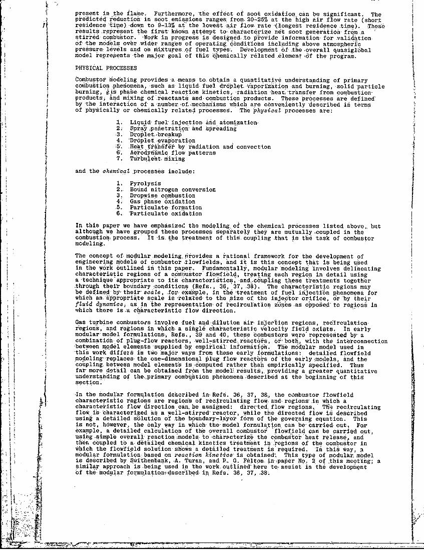
present in the flame. Furthermore, 'the effect of soot oxidation can be significant. Thepredicted ie'ductioh, in soot emissions ranges, from 20-25% at the high air flow rate (short

7 residence tiihe),'down to'9-13 % at' the lowest-air flow, rate (-longest residence .time). Trheseresultsrepresent the first kfiown 4ttempt to characterize net soot generatioh-from astirrae-combu'stor. Work in progress is designed, o provide information, for .validation,of'the models over wider ranges of operating,'d0ndit'ions inxcluiding above atmosphericpressure: levels and on mixtures-,of fuel types-. Development of the overall quasigl6balmodel represents the -major goal of, this dhemically related element 6f the, program.

PHYSICAL PROCESSES

Combustor modeling provides-a means to. obtain a quantitative understanding of primarycombustion phefiomeha, such as- liquid fuel 'dr6pletV'apori'z'ation -,and burning, -solidparticleburning, 4is phase, chemical-reaction kinetics,, -adiation-heat, transfer from combustion-products, and mixing ofreactants and- combustion products. These processes are defined'by the interaction of- anumberof.mechanisms wfiich are c6nveniently 'described ini termsof physically or chemically related processes. The physical processes are:

1. Liquid-fuel injection And atomization,2. Spray pefietration', and spreading3. Dro let,,breakup- J4. Dropietoevaporation5. .H1eat tri.'fer by'radiation and convection6'. Aer6dynafinic flowpatterns7. Turbuljnt, mixing

and the chemi'cal processes include:

1. Pyrolysis2. Bound nitrogen conversion3. Dropwise combustion4 Gas phase Oxidation-5. Particulate-formation6. Particulate oxidation

In this paper we have emphasized the modeling of the chemical processes listed above,, butalthough we have grouped these processes separately they are mutuallycoupled in thecombustio:process.' It ,is- the treatment of this. coupling-thnt is the task of combustormodeling.

The concept of, modular.modelingpriovides a rationai framework for the development ofengineering models of combustor,tlowfields, and it is this concept that is being usedin the work outlined in this paper,. Fundamentally, modular modeling involves delineatingcharacteristic regions of a com.6ustor'flowfield, treating each region in detail usinga-technique appropriate to its characteristics, and*,c~upling these t'ieatments togetherthrough their boundary-conditions (Refs., 36, 37, 38). The characteristic regions maybe defined, by- their scale, for, exawple, in the treatment of fuel ifi ection phenomena forwhich an-appropriate -scale is -ielated-to the size of, the injector orifice, or'by theirfluid dynamics, as in the representation'of recirculation zones-as opposed to regions Inwhich there isa characteristic flow direction.

Gas turbine combustors involve fuel, and-,dilution air, inje°P'ion regions, recirculation,r egions, 11and regions -in which, a single c haracteristic velocity field ,aists, In earlymodular-model formulations,,Refs., 39'and 40, these combustors were'represefited by-acombinatioh,f plug-flow-reactors,,well-stirred, reactos, orboth, with the intirconnection-between model elements-supplied-by empirical informatdh. The m6ular model used in'this work"differs in two major ways from these early formulations, detailed flowfieldmodeling,replaces-the one-dimensional plug flow reactbrs of the early-models, and-thecoupling, between model elements is ,c'mputed rather than empirically specified. Thusfarmore detail can be obtained from the model results,, providing a greater quantitativeunderstanding of the,,primary combustion phenomenadescribed at the beginning of this

section.In the modular formulation described in-Refs. 36, 37, 38, the combustor flowfieldcharacteristic regions are regions of recirculating flow, and regions in which acharacteristic flow direction can.be assigned: directedflow regions.' Tfei, recirculatingflow is characterized as a weil-stirred reactor, while the directed flow is describedusing a detailed s6lution of the b6uhdary-layer form of the -governing equation. Thisis not, however, the only way in. which-the-model, formulation can be-carried- out, Forexample, a detailed calculation of the overall combustor 'flowf-eld can be carried out,using-simple overal-,reaction-models to',chargcteriz the cobustoi'heat release, andthern coupled to a d'etailed chemical kinetics treatment in-regions of the combustor inwhich the flowtield solutionsiows'a detailed treatment is required. In this Way, amodular formulation-based on reaction kinetics is obtained' This type of modular modelis described by SPithenbank,,A. Turan, and P_ G. F6lton, in paper No'. 2 of this meeting; asimilar approach is-being'used in the workoutlined here'to assist in the development' 0~~f the~modular . . .formulation-,described-in.Refs.' 36, 37,.38'."

Zi777 41_-7777

~CLOSURE

'The information -being generated in this program provides an improved understan-g"' of-the processes, important to, alternate fuels utilization,- The "end item" is afi iar.alyticalmodel which allows -prediction of -fuel effects in various:'tkpes of continuous -c6mbustiotxdeVices, particulafly gas turbines. Such a development will provide combustor designerswith a tool, to develop fuel -flexible combustion systems whibh can utilize syiif u6s -which-are produced6 with minimum refining/upgrading and, -hence, minimum cost and. energy consumptionduring refining. .

REFERENCES

i. Jackson, T. A..,. and, Blazowski, W. S.., "Fuel Hydrogen Content as an rndidat6r- ofRaditive Heat :-nsfer-in an Aircraft Gas Turbine Combustor, in s-T'ibnCombustion -and Fueis Technology, ASME, Unit'd-Engineering Center, 345 E.-47th St.,New York, N.Y., November 1977;' pp. 59-65.

2. Dodds, W. J., Peters, J. E., Coklet, "M. B.. and Mellor, A. M., "Pieliminry Study ofSmoke Formed in the-Combustion Of-Various Jet Fuels,'," J. Energy 1, (2), March 1977.

3. Bartok, W., Engleman, V. S., Goldstein, R. and Del Valle, E. G., "Basic Kinetic Studiesand Modeling of NL Formation in Combustion Processesi" AIChE-Symposium Series 68,(126) , 1975, p. 30.

4. Street, J.-C., and Thomas, A., "Soot Formation in Premixed Flames," Fuel, Vol. 34,1955, pp. 4-36. -

5. Daniels, P. H., "Carbon Formation, in Premixed'Flames," Combustion and Flame, Vol. 4,1960, pp. 45-49. -

6. Tesner, P. A., "Formation of Dispersed Carbon by Thermal Decomposition of Hydrocarbons,"7th Symposium on Combustion, 1959.

7. Chakraborty, B. B,, and'Long, R., "The Formation of Soot and ,Polycyclic Aromatic Hydro-carbbns in Diffusion Flames III;'Effect of Additions of Oxygen to Ethylene and Ethane

-Respectively as Fuels," Combustion and Flame, Vol. 12, 1968, pp. 469n47-6,

8. Homann, K-. H., "Carbon Formation in Premixed Flames," Combustion and-Flame, Vol. il,1967, pp. 265-287.

BCURA Monthl Bulletin, Voi. XXII, No. 12, November-December 1958, pp. 48*7-506.

10. Clark6, A. E., 'Hunter, T. G,, and Garner, F. H;, "The Tbndericy 'to Smoke of: OrganicSubstances of, Burning;,, J. Inst. Pet., Vol.32 ,pp. 627-642.11'. MacFarlene, J. J., Holderness, F. H., and'Whiteher, F. S. -., -"Soot Formation Ratesin Premixed Ca and C6 Hydrocarbon-Air.Flames-at Pre sureUp tb 20 Atmospheres,"

Combustionand Flame, Vol..8 1964,,pp 215-229;

12. Schallp., R. L., and Hibbard, R. R., "Smoke and Coke Formation in the Combustion ofHydrocarbofi-Air Mixtures," Chapter IXin,"Basic, Considerations in the Combustin, ofHydrocarbon- Fuels wLth Air.," JNACA Report 1300, 1957, pp. 242-255.

13. Fennimore, C. P., Jones, G. W., and Moore-, G. E.,, !'Carbon- Foimation in Quenched FlatFlames at 16009Ki" 6th Symposium (International-) on Com ftion, 1956, ;p. 242-246.'

14. Stehling, F. -d., razee j-J. E., and Andersoi, R. C. , "Carbofi- Formation, fr6em Acetylene,6th Symposium (Ifiternatiofal) on Combustion, 1956, pp; 247-254. - - "

15. D'Alessio, A.-, DiLorenqzo, A-.-, S~rofim, A. F-., Beretta, F., Masi, J., and Venitozzi, C.,"Soot Frmation in CH4-02 Flames, W15th Symposium (-Interhationdl) on Combustion, 1974,* 1 pp. 1427-1438. - ..

16. Palmer, H. B., and-Cullis, C. F., "The Formation of Carbon from Gases," Chapter 5 in•Chemistry and Physics 0f. -Carbon ,'.ediied:-by, P.-L.' Walker, 1965,

17. Schalla, R. L., and :McDonald, G. 2.,- "'Mechanism of Smoke Formation, in Difusion Flames,5e.Sm~im __kjntonAY on -Combustion, 1654-, qp.' ,16,323.,

18. Artur, J. R, arid-Napier, D. H., "Formation of Crbon, and Relsald Materials in DiffusionFlames " "thS mpOsi'u ,(International) -onCombustion, 1954,, 303-315. S ,

19. Gaydon, A. 0., and Fairbairh,- A. R., "Cdf~bn -Formation in, C2 and 'CO in :Discharge,194 p,324-328.1. Wight, F. J., "Effect of Oxygen- b h the Carbon Forming Tedencies of Diffusion lames,,

Fuel, -Vol;,53-No. A,06tober 1974, pp. 232-235. -F.a.es,"

7- r- 7-

21.Schrme, RM,, "ffect of Fuel Coffpositioh'ofi Particulat Emssions from Gas

21. in .nie.,A Emissiohs f rm-,Conitinuous Combustion Systems edited I by W.

'ICoinelius and W. G. Agnew1. Plenfum'Pressi 1,972,p'18-20

22. -Magnusson, B. F., "An Investigation into the Behavior of Soot in a Turbulen-t 'FreeJet C2H 'Flame," 15t1L,,Symposiini ('internationai) 'on Combustion, 1974, ,p. 1415-1425.

2.Wright, F. J'.j "The Fbrmatiorrof 'Carbon 'Under Well-Stirfbd-Conditions," 12th Symposium-23. (nternational) on Combustion, TheCombustion Institute,.yPitis~burgh, Pa., 1968,

pp. 6-8b

24. Wright, F. J , "Carbon.Formation Uider Well-Stirred Conditions, Part II,"1 Combustionand Flame; -Vol. 115, 1970, pp. 217-;.22 2.

25. Jenson, D. 'E.,, "P rediction of Soot Formation Rates: A New Approach," -Proc. Roy. Soc.London, A. 338, 1974, p. 375.,

J 6. Tesner, P.A., Snegiriova,- T. Dand .Knoine, V. G.,, "Kinetics of Dispersed CarbonFormation," Combustion afid-Flame, 17, 1971, pp. 253-260.

27. Khan, 'I.. M.., and Greeves, G., "A Method'.For Calculating The Formation and Combustionof Soot in Diesel Engines,".Heat Transfer From Flamds, N.UfaanJ.M-erEditors, 'Scripts.Book Co,/Halitead>pre6s , 1974, pp 38-44.AfaanJ.M Br

28. 'Edelman, R. B. and Harsha, P., T.,, "'Laminar and Turbulent Gas Dynamics in Combustors-Current Status," Progress ineEnergy an'd'Combusti6n Sciefice,.Vol. 4, 1978, pp. E-62,

29. Lee, K. B., Thring, M. W., and. Beer,,J. 'M., "On the Rate of Combustion of Soot in

a Laminar Soot Flame," Combustion and 'Flame, Vol., 6, 1962, pp. 137-145. ________

30. Nagle, J.,.Strickland-Constable, R -FR.~, "Oxidation ~of Caikbon Between 1000- 20000C,"1Proc. Fifth Carbon Conf., 1., 1962,, p." 154.

and Flame, 20, 1973,,p. 369.

* 32. Longwell, J. P. and Weiss, M. AX., Ind. Ehg. 'Chem.,, 47, 1955, p. 1634.

33. Blazowski, WN. S., "Dep'endence of Soot Production onFuel Blend Characteristics andCombustion Conditions," ASME Paper 79-GT-155, 24th I-nternational1 Gas TurbineCoh'ierenc6, March '1979; *.o be published' in ASME.Triansactions.

34. Graham, 'S-.C., Homer, J. 'B and Rosenfeld, J. L. J., "The Formation and;Coagulptionof Soot ,Airosols," Int. Shbc: _Tube Symposium,' 10th Proceedings, (1975).

35. Graham, S. C., Hom~er J. B.-, and Rosenfeld, J. L. J., "The Formation aid' Coagulationof Soot Aerosols' Generated by the<Pyrolysis~o Aromatic Hydrocarbons," Proc. Roy. Soc._London A., (1978) Vol.,344.

36. Edeliian, R. B. -and Harsh'ai P. T., AFOSRt Interim Scientific Report, "Mixing~and' Combustion in High Speed 'Air Flows," AFOSR-TR-78-0878, (SAI-78-008-WH), ScienceApplications, Inc., April 1978 (AD-A054398).

3.Harsha, P. T., and Edel Iman, R. B.,, "Applition of Modular Modeling to,-RamjetPerformancePrediction," AiMAAPaper 78-944, July 1978.

38. Harsha,.P. T. and Edelman, A. B., ',IAF0SR InterimScientific Report: Mixing andCombustion in High, Speed Air Flows'," Rejbrt SAI-79-013-VH, Science Applications, Inc,,W'$odland Hills, California,, )JAi'1979.

39. 'Swithenbank, J.j, Pol~l I.,. Viiicent, 'M. WN.,, and yright, D.,D., "Combustion DesignFufidalmentals,1 Fourteenth , Symposium',(Int~rina'tional) on Co'nbustion, The Combustionlhstitufe,'Pittaburgh, 1973, 'pp. d2-66

'40. Roberts§,.R. A., Aceto, 'L. L., Kollrack, R.,, Teixeria, 'D. P., and Bonnell, J. M.,"Ah'Analytical Model for Nitjric Oxide Formation in a Gas~ Turbine Combustor," AIAAJournal, Vol._1l0, 'Nb. 6, June, '1972.

'A'KNOWLED6)EME9T

-This work wets supported'by the U.S. Departmet of Energy, Division of~ Fossil FuelUtilization (Contract No. 'EC-77-C-03 -1543). Dr. J..Birkeland of DOE 'is the responsibleProgram Manager 'anhd Dr. -. Fisher of Argonne National'Labr .oy steTehi~ rga

'try isteTcnia igMonitor.

cyjcl o iexanse'~~ 0.1 03 TT.0

~2.6

0 10" 15 2 0

p. ycliHxene N

3. 2A4',6 -( 0

LU 2.0 71 - 0.

1j .0

0 - 5 10! 1 10I 'JR~nii eSUE.AM

~1 __ _____ ____ _____3.0_Tiue I. feto Pesr n-itr t'nt

0soo foraton rato5 FrmRe2ece30

:E SSCE R , 'A TM.U~L~RECO

Figur 2. xpermentl gr-itio Dlay Timt, DathePrditons fo atii tesad Cyclicber

TypnHdrcarb onsifn rdli f ,lntn)ioo /omtinrto)Fo eeec 7

.12.0 1.

I010.0

0? JSC Oia Prgec ion"'Prediction .

i Exxon Data-Jet Stirred oc ustor

0OData6.0~ 0 0

A ~.0

2.0-

0 O. .4 0 0.2 0.4 0.6 0.8 1.0

Equilvalence Ratio,

(qutnalenci Rifo. 4Figure 3. Comparison of Prddicted and Figure 4-. Comparison of Predicted and

Measured-O Concentration, Measured CO. Concentration,Isooctane. Isdoctane.

-.o-; Isooctana

..A..Toluene

• .- Ethlene

• -- 'PO.{ICTIO, ,sooctane

1.00 -. 10

0 7 M ea su re d Hy d ro c a rb o n C on ce n tra tio n .2 51

• ,

I , /, g C, - lto0. - d, .08 o- # - 0.4,0. . .06'-

0* I * v I d - -,a... - o' O 0 -t J

o . -0.2z .,..4 o .6 --0.6 .0o "-o., o. " o. "- o.s 1.0

i~igure 5. Comparison of. Predicted~with Figure 6. Comparison of Predicted and Measured

Mesre CQoc.ti s Hydrovarbih Concentration, Isooctane.

.01 -

•~ D-ata

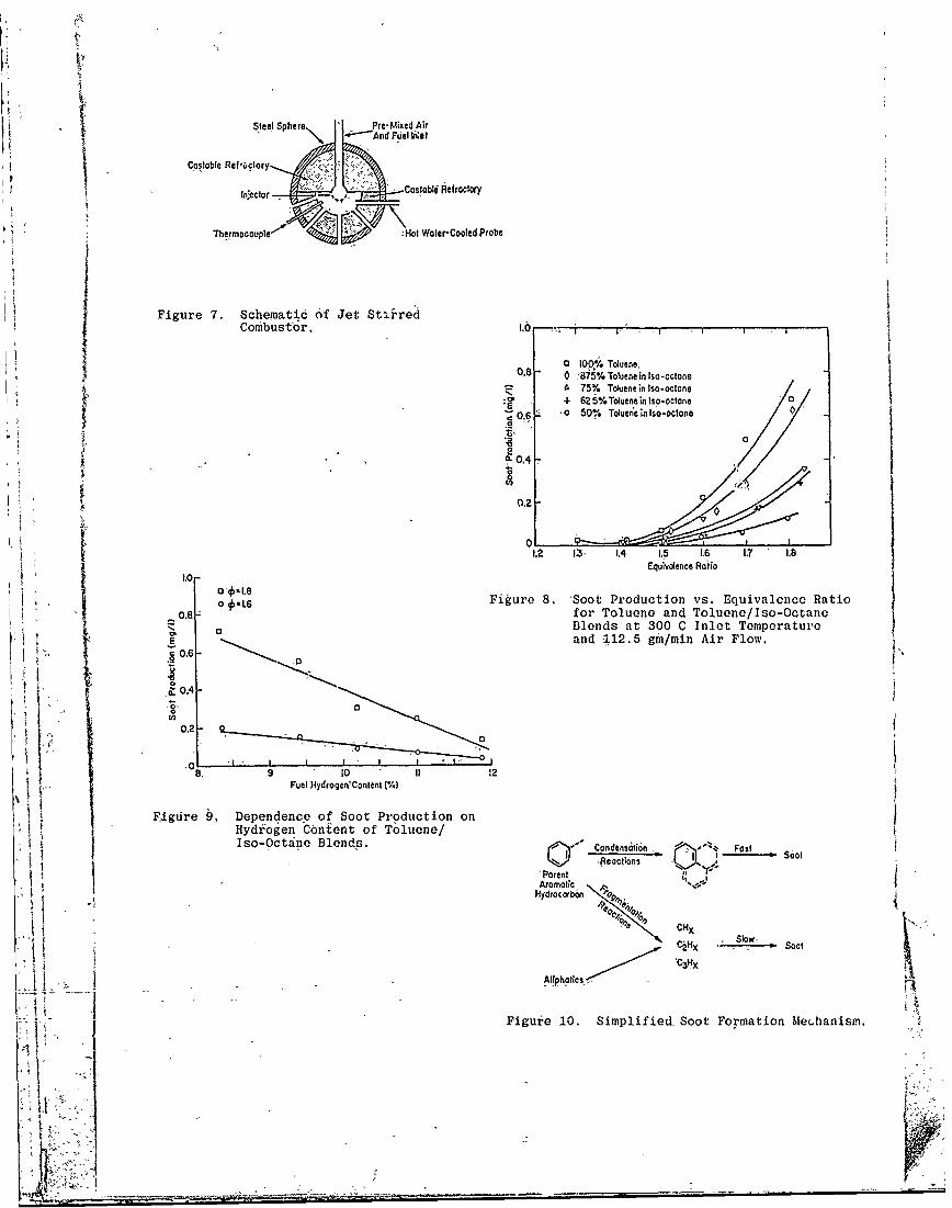
Stee Sphere Pre-Mixed Air

Ca oble Rellucory S-- An e

Injector uobi .-- efroctory

Thermocouple' M " . Hot Woler-Cooled Probe

Figure 7. Schematic of Jet Sti'redCombustor. 10F , , -,

0 I0P,*. Toluene,0 875% Toluenein Iso-ocone0.8 75% Tolueneilso-octone

+ 62 5%Toluene in Iso-octone '0'E o 0 0 50% Toluene inlso-octone 0

0 t 0

0.4 -

1.2 13, 1.4 1.5 1.6 1.7 1.8"°0 Equivalence Ratio

0-,6 Figure 8. 'Soot Production vs. Equivalence Ratiol oe for Toluene and Toluene/Iso-Octane

Blends at 300 C Inlet TemperatureSE and 112.5 gm/mlin Air Flow.

, , 0,6 0

oA 0

00• I IC I - I " I" I18. 9 10 II 2

Fuel Hydrogen'Conlent 1%)

Figure 9. Dependence of Soot Production onHydrogen Content of Toluene/Iso-Octane Blends. P Condens6ton - ," Fas

t Parent I. l- - - SooAromatic x %,I

Hydrocarbon C

CHx '

CiHx * -.- Soot

'C31.tAliohatics

Figure 10. Simplified, Soot Formation Mechanism.

i'l

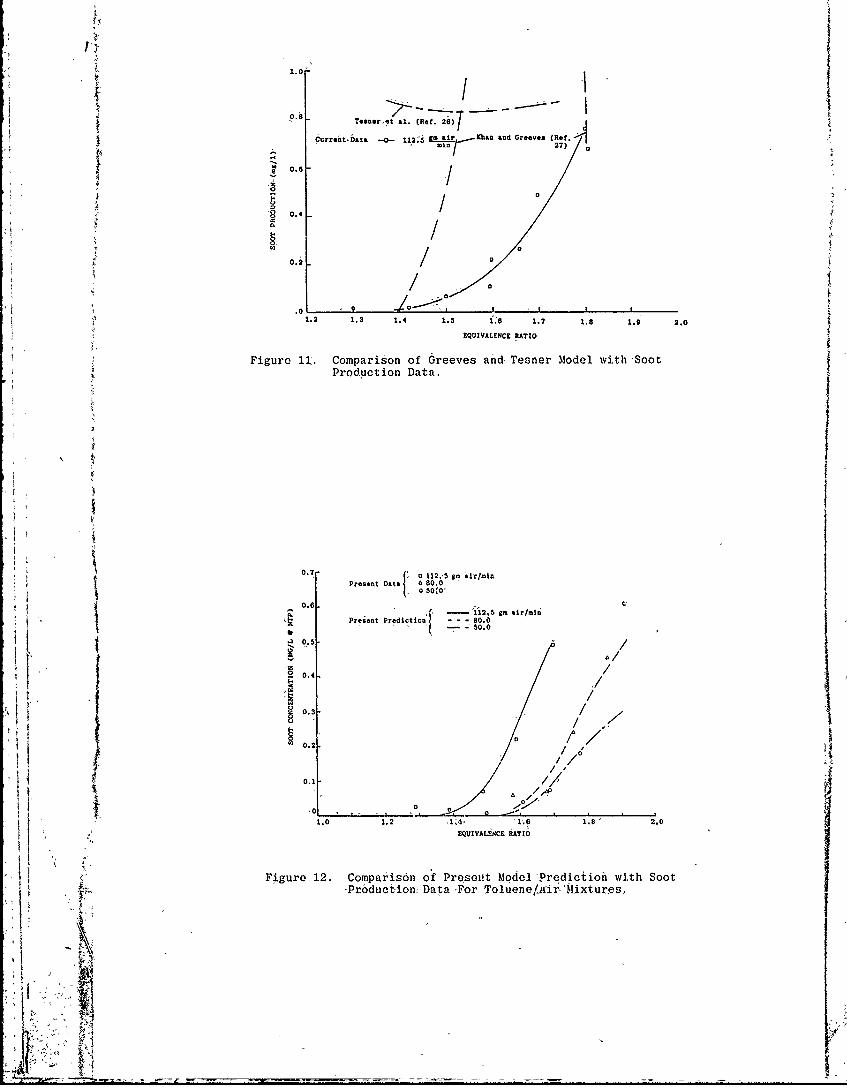
j Tesner~et al. (Ref. 2i)[

C.!. --.

' K h a n and Groeves (Ro,

Cur~nwint -.- 11. 27) n

I 0

.~2

0.6

0

.01I1.2 1.3 1.4 1.5 1'6 1.7 1.8 1.9 2.0

EQUZVALENCE RATIO

Figure i1. Comparison-of Greeves and- Tesner Model with SootProduction Data.

0.7 1 0 112,S gm iir/ inPresent Dta 4 80.0

I 050.0,

0.6.06 Prevent Predictlo - - - 80.0

- --- -°50.0

91 0.5-

: /0I

0.2/0-

1.0 1.2 1 4 1.6 1.8 2.0

EQUIVALE14CE RATIO

Figure 12. Comparison of Preset Model Predictiohi with Soot-Pr6duct-ion: Data -For Toluene.air-'Rixtures.

_N~

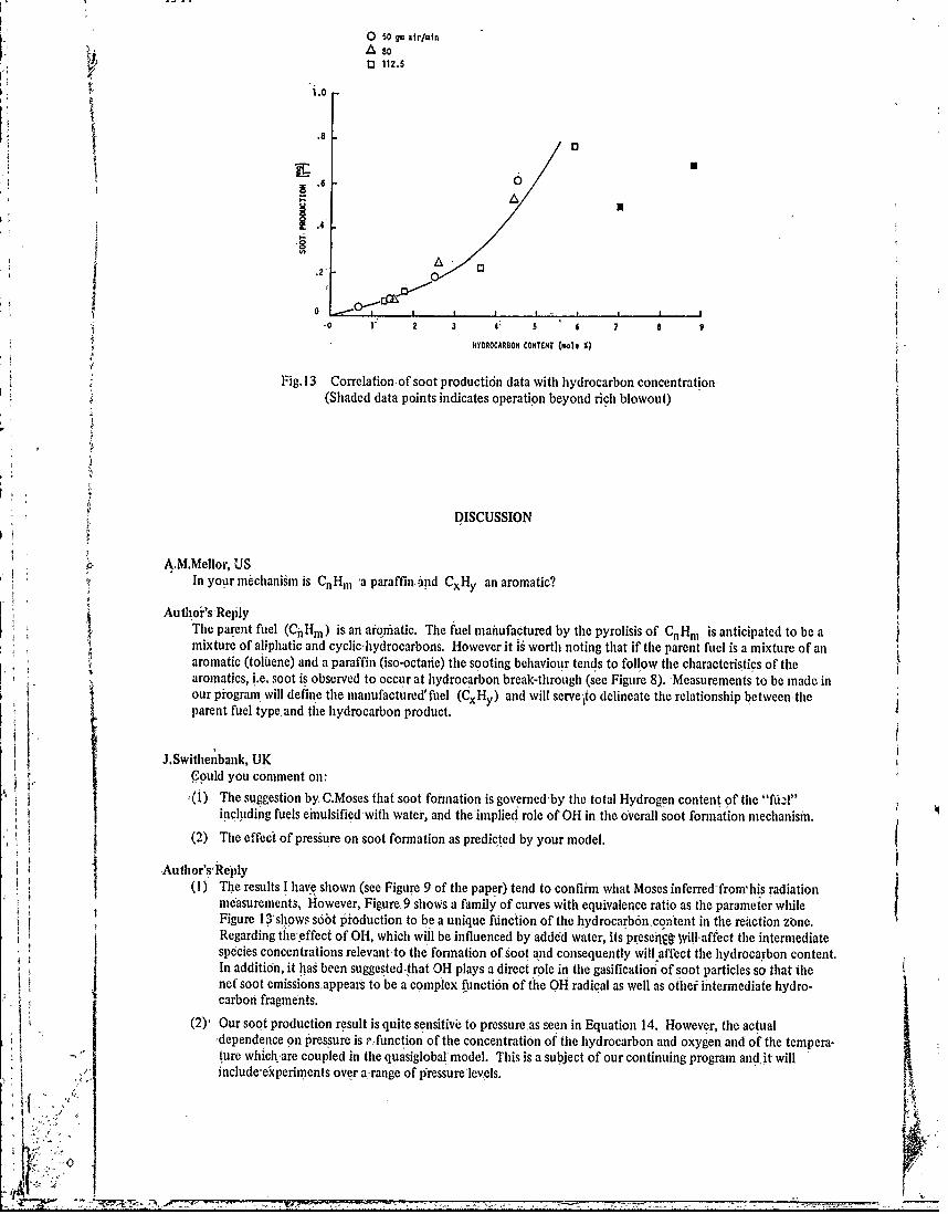
0 50 9m air/min~A so

- 112.5

0PA

.4'

.2 /E3

V o " 2 3 4=

5 6 7 a 9HYDROCARBON CONTENT (mole %)

Fig. 13 Correlation-of soot production data with hydrocarbon concentration,(Shaded data points indicates operation beyond rich blowout)

DISCUSSION

A.M.Mellor, USIn your mechanism is CnHm a paraffin,-nd CxHy an aromatic?

Authoi's ReplyThe parent fuel (CnHm) is an aronatic. The fuel manufactured by the pyrolisis of CnHm is anticipated to be amixture of aliphatic and cyclic hydrocarbons. However it is Worth noting that if the parent fuel is a mixture of anaromatic (toluene) and a paraffin (iso-octafie) the sooting behaviour tends to follow the characteristics of thearomatics, i.e. soot is observed to occur at hydrocarbon break-through (see Figure 8). Measurements to be made inour program will define the manufactured'fuel (CxHy) and will serveito delineate the relationship betwcentheparent fuel type~and the hydrocarbon product.

J.Swithenbank, UKCould you comment on:

1(l) The suggestion by, C.Moses that soot formation is governed'by the total Hydrogen content of the "fu.l"including fuels emfulsified with water', and the'implie d role of OH in the overall soot formation mechanismn.

(2) The effect of pressure on soot formation as predicted by your model.

Author's~Reply(I) The results I have shown (see Figure 9 of the pAper) tend to confirm what Moses inferred-fromihis radiation

measurements, However, Figure,9 shows a family of curves with equivalence ratio as the parameter whileFigure 13'shgws soot pr'oduction to be a unique function of the hYdrocarb6n~on'tent in the reaction zone.Regarding theeffect of OH, which will be influenced by added water, Its presei' Wyillaffect the intermediatespecies concentrations relevant-to the formation of soot and consequently will affect the hydrocarbon content.In addition, it has been suggested that OH plays a direct role in the gasification'of soot particles so that thenet soot emissionsappears to be a complex function of the OH radical as well as othei intermediate hydro-carbon fragments.V (2), Our soot production result is quite sensitive to pressure as seen in Equation 14. However, the actual,dependence on pressure is ?.function of the concentration of the hydrocarbon and oxygen and of the tempera-ture which are coupled in the quasiglobalmodel. This is a subject of our continuing program and it willincludeeperiments over a-range of pressure'levels.

'7 :77

CHEMICAL KINETIC MODELLING FOR COMBUSTION APPLICATION

F.L. Dryer C.K. WestbrookMchanicl -and Aerospace Engineering Lawrence Livermore Laboratory

Departnent and Livermore, California 94550,U.S.Princeton UniversityPrinceton, New Jersey 08544, U.S.

SUMMARY

Chemical kinetic modelling of combustion in practical energy production systems isdifficult for seveial reasons. First, very little information is available concerningi the mechanistic details of fuel pyrolysis and oxidation- for most typical hydrocarbons

fuels. Secondly, intiOse few cases wheremany-of the elementary reactions are known,rate data ae-generally unreliable or completely uiknown. -Finally,, the large -sets -ofchemical- rate equations which'arise are difficult and expensive to solve, even on themost pdwerful-computers,. when they are intimatelycoupled with fluid dynamics. -As aresult of these considerations, 'the conventional approach in.many cases has been touse greatly simplified themical kinetics models which avoid many of the above problemsby-confining attention only-to the overall rates of fuel consumption and heat release.While-extremely useful for'interpretiVe calculations, this type of approach has beenfound' to hav certain significant limitations. The simplified models--do not extra-polate well7to'conditions 6utside those for which the-model itself was derived, quen-ching phenomena and pollutant formation are poorly described, and other results com-puted by such models can be misleading.

This paper describes the results of a-systematic program-denigned to producekinetic models for practical fuels. There are two prindipal goals -to this'work,, bothof which are immediately relevant to efficient combustor design; The first goal isthe construction of detailed reaction mechanisms -fo the oxidation of typical hydro-carbon fuels, and the valldation'of these mechanisms through careful comparisons be-tween domputed and experimental data. These mechanisms are strongly hierarchical,with reactions for complex fuels containing subsets -which'describe the combustion of-chemically simpler fuels. Progress to date includes relatively complete descriptionsof carbon monoxidehydrogen, methane, ethane, andmethanol oxidation. In the develop--ment and verification of these reaition.me'hanismswehave aftempted to use data froma variety of experimental sources, including flow reactor techniqu~s, at intermediatetemperatures (960 -' 130O K) and shock tube results for high temperatures '(1300 - 2200K).In addition, ranges in fuel-air equivalence ratio between very lean ( < 0.1) through-stoichiometric-to very rich ( > 5) have been considered, all intended to make the

models derived in this study as general as p6rsible.

* In addition to the-direct utility of detailed kinetic models, such-descriptionsare very useful 'in the derivation and validation of appropriate -simplified reactionschemes for-practical fuels. Simplified models derived from detailed~mechanisms'arepotentiallymore general than those derivedentirely from-,experimental correlations.Furthermore, the additional kinetic insight gained by this approach can also provideadditional insight into the operating choraltistics of- simplified mechanistic methods.

INTRODUCTION

Numerical modeling is rapidly becoming, an essential part of many combustion re-search'programs. For a number of years Aumerical models have been-used-to assist inthe interpretation of specific laboratory-scale experiments. Inaddition, computeranalysis of idealized problems has provided useful insfghi into combustibn zproblems

i whichhave been too comple:X,to approach on an experimental *basis. Yet,, the eventual

goal of more recent numerical work is the construction 'of representations which canassist directly, in the design of-practical combustbrs, i.e. which would-be predictive

swell s interkpretive, Giventhe'widerange of operating parameters experienced inmost conventional-combustion sft~ati~ns,_ It is clear that a 'suitable physical and hu-merical model ifor each of the many physical and chemical processed (at6mization, vapori-zation, iurbulence, heat transfer, chemical kinetics,,etc.) must be-embodied in thisrepresenitation. these "sub models must predict the independent phenomena -as Iwell as

t crret 'coupling of iatious physical and-Chemical pr6cesses (e.g. turbulence andchemistry)* Furthermore, calculations must be reliable even in parameter ranges where'experimental data are not available to validate the predictions, Such numerical toolscar be exceedingly valuable, reducing,'both the cost and the time required for'thd de-~entof combustion systems - Here W6 Wi§i t6 foCtso on some aspects of the construc-

ti the sibmodel for utombuion chemistry. .. ..

It shouldbe recognized from 'the beginhing thatregardless of the apparent sophis-tication of some repesentations, all existing chemical kinetic models are in -realsense Event th' Eieost-detai"'d-el~rhentary chemical kinetic-mech-anisms,which have been deeloped (6.g. those for H2, CO, CH4 oxidation) are constructedon the basis of r6prduc ng'6bserkable pheomena which are 'not all-encompassing. Formorecomplex fuels, only limited kinetic informatinis avallable. Inideed-in the caseof aromatics, eien the important species and elinentark reactions remain in doubt. Fur-thermore, the 'aluation of specific rate constants (oi oveiall reaction) over ranged9f temperature and pre.s-re adequate for combustion modelling is a ever present'

------ - ------- -------- --- --------------------- ._ _ _ __

potential source of error.

In the following sections ,we shall discuss several techniquesfor describing thechemical kineticbehaVior'of €oibustion phenomena. At the simplest level have bee' theuse of flame speed or single step heat release correlations. Such correlations may becast as global or overall rate equations. For exaple, Butler et al. [l] have repre-sented the combustion of n-0ct'ne as

2 C8 H1 8 + 25 02 16 CO2 + 18 H20

-9.38 x 10lpfPo exp (-15, 780)f) cfp ex g/cm32

where the subscript f refers to-the fuel and the subscript c indicates the change inpartial density due only to chemical reaction. Even, simpler in kinetic terms is thespecification of the rat of reaction as a function'onlyof time. The functional de- Ipendence is derived from- experimental, data and ued As, input to the overall model. *nexample of this type of description is given by Blumberg 12] for combustion in strati-fied chargeiengines, where the fraction .c bf the mass-whfch is burned, expressed as afunction of',crank angle', is, ien:by

a (0 _ i 2 Cos,'1-0- 0/1

where A66 is the interval over which-the combustion is assumed'to take place. Theseapproaches have bekn, frequently employed in combus ion modeling nd-'have -often. been '

'founhd to be adequate for interpretive calculations of overall systdm'performaice.

However, description of'hydrocarbon combustion chemistry in substantial detail isrequired when considering a number of other practical combustion problems of 6urrehtinterest. These include:

* -trandition to fast chemical -reaction

A) spark ignitionb) compression ignitionc) engine detonationd) transition from-deflag;ation to -detonation%j) exp1osion,

* Flame.quefnchifig and hydrocarb6n.6ission

a) by-wallsb) by. charge stratificationc) by- rapid expansion

* Flame inhibiti6n_6nd extincti6n.

* Fuel nitrogen conversion

0 Thermal NO production within fiame.,btructures

i • S02/S03 conversion in post-flame-gases

o Soot formation, particularly for aromatics

0 Soot oxidation

* Catalytic,processes

in these areas, the:chemistry and ,other submodels'are generally coupled 61osely, andfluctuat:ions in 'local enthalpy and species concentrations become. important. Indeed, oneprobably cannot 'suitably model turbulentcombustioh with6ut a detailed tieatmenit of thecombustion-chemistry. However, we shall for this'presehiiion eiclude consideration ofkinetic'/turbulence coupling. The importance Of, this problem, is clearly recognized. It-has more recentiy been common to attempt validation of turbulent combustion models inwhich the chemistry submodel" 'is known to'be unreaiistic. We believe the problem cannotbe dqfined Adequately without first'assembingturbulence and chenistry models whichcorrectly predict uncoupled .phenomena.

- in addition to difficulties in constructing a detailed chemicalmodel its use isliiited by seveal severe pioblems associated'with the computer solutioenof thecoupledchemistry/fluid mechani'csequations. These problems are all related to the fact thateven.'the best current scientific computers have size andspeed limitatiorns which cannotbe neglected. In, the most-.direct-niethod of formulation, the concentration of each chemi-cal species in the reaction mechanismsi is repvesented by a Single lifferential equatiq'n;common techniques then replace, this diffeiential equation with.a finite'difference equa-tion. If the problem is 6nein:'which.only chemical kinetics need be, considered, ne-Ii I, oived isequa -t thenuerospcs tgte whn teuatinerfo energyn o'en iglecting'spatial vaiations-of'physical quantities, then the number of equations tofbesolved is equal' 'to the -number of spcies togetien -with a'n eergy -or en-thalpy. 'Such sets ofc6upld difference equations (coupld' through nonlinear reaction

~~j~i2. rate termfi)'..Are' alreadi~y often difficult t o-ihnef'fietanacute'ner

" "to- _ov _a _, _e a-r

14-3

When spatial variations of, allquafntities are included in the model, 'then'differenceequations foa a 1 species anh'd nerg musthbe 6s6lid"'at each point in the physicaldomain, usually'--epresdn 'd initediffernce spatial mesh. The' total nimber ofequations to be solved, the aimont of-computer timereqhifed, and the" computer storagerequirements increase veryrapidly . All of'these liits are severely tested even forapplications in-which the spatial variations are limited to one dimension. For problemswith two-"and-three-dimensiohal .spatial variations; reaction mechanisms"wibth many chemi-cal species (>10) are probably too-slow 'and expensive in terms of -computer requirements.This is partic-ularly trueif one needs- to- perform any typ6'of parametric numerical study.Thusso kind ofmechahism.simplification, must :bed considered for these cases.

These simplified mechanisms 6kftei lid between the two extremes of model complexitydiscussed above, and in addition to idehtifyIng some of the key properties arid limita-tions of detailed and -global reaction models we, shall dis'cuss at some length 6ne' of, themore opular simplificati6n approaches which have been poposed. Thediscussions belowdepend heav'ily on our earler work' [3,4,516,78,9] 'to illustrate these characteristics.Let us begin by first addressing the most complex approach, that 6f-detailed mechanisticmodelling.'

DETAILED KINETIC MECHANISMS

Table I gives an example of a comprehensive detailed chemistry mode]. This reaction*mechanism for methanol oxidation which we have recentlyderived,[3], accurately repro-

duces observed experimental chemical kinetic behavior for various experiments over thetemperature range 1000-2180 K, ,the pressure range-1-5 arm, and the-equivalence ratiorange 0.05-3.0.

Examination of Table I provides some insight into the structure of detailed mech-anisms for hydrocarbon'oxidati6on. The methano oxidation mechanism consists of 84 ele-mentary reactions '(each of which includes~a finite rate in both the forward and reversedirections) involving 2- chemical speoies. If NOx chemistry were to be considered',another'4 'species (N, NO, N02, -N20) and 10-15 reactions would be required. Considera-tion 'of fuel'bound nitrogen i the form of NHi. or HCN would require a further enlarge-me-t of the mechanism.

' Reactions 40-56 provide a reasonably complete description of U2-02 mixtures, andtogether and withreacibns' 36-39, aze adequate to- describe carbon-' 6hoxide-oxidation,in the presence of water'vapor. Experiments carried but "in the Princetdn Universityturbulent flow reactor for CO oyidation [10] at atmospheric ressure and -1000'K have-been accurately described with this reaction4mechanism [7]. Figure 1 compares experi-mental and calculated resuits fr 'the temperature, 'CO mole 'fraction, and CO2 mole ,frac-tion, all plotted as functions o-f distance (time)' from the plug flow reactor inlet.The agreement between computed and, experimentl data for this one-dimensional reactionzone is excellent (Fig. lb)., It is interesting to note that when reactions involvingHO2'andtH202-(Ractiois 44.and 46-53) are omitted from the reaction mechanism, the mo-del predictions'do not agrei;weli withi-xperimeht (Fig. la). The'importance of HO2 andH2 0 2 in CO systemw 'has'rot been, commonly appreciated (6), but it is clear 'from Fig. 1that even the relatively simple case of CO 6xidat':n is substantialliymodified by thesereactions. It has often been suggested that' these reactions, abre unimportint-in-combstion,systems at temperatures above 1000 'K. However, recent work [6] has shown-tlat thesespecies remain important for temperatures up to 1800 K at elevAted pre'ssure (P > 10 atm).Weahave also recentlynoted a key role these species play in d {terminirigthe'pr~ssure de-pendeThce of laminar flame velocity [9].

Reactions Ii-35 and 57-84, together with the CO-H2;O 2 mechanism, comprise a methaneoxidation mechaniiim which hasbeen used to describe turbulent flow reactor iesults (7].

!yp* c~l. results, are shown ,in Fig. 2. 1In' thi s study it was foufid~that 'even for very lean0.05) methn6 oxidation, it is important to include methyl radical recombination

CH3 + 'CH3 C H

andethane oxidation reactions, The methane oxidation mechahism has been further applied

to.istudies of the -hock tube ignition of mixtures of methane and ethane [8,11] in ordertb ,assess the poSsille dangers of detonability in mixtures of liqified natural gas (LNG)an air. Some' of these results are shown in Fig. 3,; in which'. e ignition delay time-of a shocked gas saiiple is plotted as a function of'reciprocal" temperature. 'The uppersolid line represehts experimental data for stoichiometric m thane-air and the lower solidIlini'for stoichiometl-,d.ethane-air. Computed ignitiondiela'y'imeS for stoiclometricmixtures of methane hane-air are siown as dashed-lines.f This study again confirms thatethane formation and bxidation isanessentill part of the methane oxidation mech.is;'

There are several. general observations to-be made with respect to the detailed re-actiop, mechanism for methane. First, it should be noted that as a result of the diffi-cultywith which methyl radicalslare oxidized, there are complexiiesn the oxidationof even ,thi& 6imple fuill molecule. When these effects are included it ". possible toreproduce experimental'data for a wide variety of conditions, ie for both flow reactor

and shock 'tube' environm6.nts. Unfortufiately, the strong dependence of the radical'poolonithe methyl radical'odidation,;ieactionsis,uucharacteristic of larger alkyl hydrocarbonoxidation processes. Thus the ,resulting lohg induction period and oxidation character ofri met~aane do not closely simulate the combustion properties of conventional liquid fuelcomponents.

<"

Computed. results for methane oxidation indicate several distinct phases or stepsduring'which different reaction groups.,control the overail rate of oxidation. Afterthe induction phase there is a period during which fuel -is rapidly converted'primarilyt. Cqi. follbwed by a phase .dominatedby the oxidation' of CO"to _02 (?ig. 2).. The maxi-mum CO-mole faction occurs at a disance'.of approximate 5 of i

the, cylindrical duct; Other ma"op intermediate Sbecies reach their maximumvalu'es atdifferent locations,. Soma of these are, c2O (20. cm)'j c 2 H6 (30 cm),, €2H4 (40 cm) and H2(45,cm).. Using the rate expressions in TableI, at flow reactor temperatures, k(CH2 +OH) >k(C 2 H6, + OH) >!"(H2 + OH) >k(CO + OH)', and similar trends appear for reactions with0 and H atoms. Ths, ordering in, reaction rates-'isresponsible for relative locationswhere the species maximum concentrationsoccur.' In fact, the hydrogen abstraction re-action rate, of any-alkyl hydrocarbon and-a hydroxyl radical is more than 100 timeslarger than the CO + OH reaction rate,.at these temperatu~res. Since nealy7 all CO oxi,7dation takes place by reaction with OH, it is clear that CO will, react very slowly inthe presence of hydrocarbons. 'The exothermicity'of the carbon monoxide 6onversic p0ovides a large fraction of the total heat of2 combustion for fuel-air mixtures' Thds,,much of the energy release 'ppearskoniy aater the, fuel and major intermediate hydrocar-bon species ha- been consumed. 'The interactivecharacter of the carbon, monoxide and,methane oxidations is characteristic of that noted for larger alkyl hydrocarbon oxida-tion.

Reactions 1-10 in Table I were added to the earlier methane-ethane mechanism andused to describe methanol oxidation [3]. -The mechanism Was shown to describe shocktube and turbulent flow reactor data over wide ranges of fuel-oxygen equivalence ratio,temperature and'pressure. Additional work showed that the reaction mechanism was ableto predict laminar flame speeds for i ethanbl-air mixtures over similarly wide ranges ofoperating conditions (9]. In order to have the capacity for making such predictions,the mechanism had to be thoroughly validated in a variety of experimental environmentsand over wide ianges of conditions. With this testing completed, ,the model predictionscan be treated with g eater confidence than if the mechanism had been able to reproduceonly the shock 'tube or only the flow reactor experiments.

Flame speeds predicted by ths model are-shown in Figs. 4-6. In Fig. 4 the varia-

tionin laminar flame speed Su with unburned gas temperature Tu is shown. Fig. 5 showsthe variLtion of Su with pressure P, and Fig. 6 describes the'dependence of Su on equiva-lence ratio, . These pediclti6ns all agree well with the available experimental data,-and a' great deal of additional information is available- from thb,'omputed. flame results.For example, the nonlinear dependence of log Su on log P in Fig, 5has been observed formany years in flames of air with methane and other fuels, but no specific process hadbeen shown to be responsible. With the-detailed calculations, it was pbser~ed J9] thatthe contributions of H + 02 + M 4 H02 tM, become increasingly important with increasein pressure, leadingto the observed fV.ame speed dependence on pressure. This same re-action character must be of similar i1p:rtance 'n any other hydrocarbon-air flame.

While we have demonstrated some of the 'favorable pr6perties of detailet2kineticmodelling, comprehens!v5 mechanisms have beefrmulated and testod for oxly a fewrelatively simple fuels. Work is~continuing on enlarging the number and types of fuels,the important elementary reactions, bit tihe solution of large ie'tworks of differentialequations can be both difficult and expensive to 'solve numerically. For practical ptx -'poses, when large detailed reaction mechanisms are used it is essontial to simplify oridealize the geometrical domain' toa single spatial cpordinate. 'Problems with two or'three spatial coordinates require prohibitive computer expenses' H~ee, many practi-cal problems which at first appear to be hopelessly two- and three-dimensional can beapproached by considering a related but simplified one dimensional problem. Such i'-p'fied studies of stratifiedcharge engine environments [12,13'], flame-quenching in ex-panding combustion chambers '14], and wall quenchihg in thermal boundary layers [15] havebeen able to provide a great deal of useful iformation through the use of detailed mech-anisms.GLOBAL REACT4ON MECHANISMS

Simpler reaction mechanisms than. those described-aboVe can be needed for sevet.1treasons. These might include limited computer faciklities, the Inecessity of using a fuel

fo Wlhi~h a -dettiled kinetics mechanism is unavailable, or, a geometry for which two- orthree-dimensional effects cannot be ignored or avoided. -.'Or such applications a' greatlysimplified reaction mechanism is needed which will provide sufficient accuracy forthegiven problem,,. In this- section we will describe briefly some of the approaches whichhave been talen;in definiig and usii'i global reaction mechai*sms.

In many applications a single reaction step can be used. As We mentioned earlier,often-the heat release rom chemical reactions is used-as ani- 'nput'quantity to the-model',

using this to determine other output quantities. 'In order to use this type of descrip-tion it is necessary to have previously carried out enough .experiments to, be able'to-prescribe the heat release function accuritely . Siice % large part of the NOx forma-tion in many combustion systemis is a function of temperature in the burned-gases, theamount of reacted gas, and the resi'dence'tim&''in, the combuston volume, this simple typeof reaction model can give a surprisingly good estimate of NOx production. In order tocbtain further kinetic detail it is necessary to make certain assumptions, such as thevalidity 6fchemical equilibrium in the burned gas,, or partial equilibrium among .theradical pboi1, etc.V

145

The most commonly used simple mechanisms are the global types, with ohe or twooverall reactions. 'The n-octane reaction discussed earlier is'an example of a singlestep global reaction. An example of a frequently used.,two;step global: mechanism isthat for methane, developed by Dryer andGlassman [10] for post-induction phase leanoxidatioh of methane in the flow reactor, at atmospheric pressure,

CH 4 + 3/2 O -,CO + 2H20

CO + 1/2 02 CO2

The,.rates for these two.readtionsaregiven by

13.2 0.7 q 0.8 3JA (CH4] exp(-48400/RT)ICH4] [ ] mole/cm -sec

d'[C 14:.75 10 0,-5 0.25 3_i -[CO 2], = 10 exp(-43000/RT)'[CO].0 [H20]0 , [O]0j 25 mole/cm 3sec.

When these expressi6ns areused to model the flow reactor experiments discussed earlierand summarized ii Fig. 2, the agreement betweenthe computer results using the simpli-fied mechanism and th6 detailed%,mechariism, is very good, as shown in Fig. 7.

These two-step global expressions have been used to model a variety of combustionsystems. Fo- example, the model yields a reasonable value of about 40 cm/sec'for thelaminar flame speed in stoichiometrIc methane-air',at atmospheric pressure; However,as the pressure is in~re~sed, the simplified mechanis i does not predict the P 0 .5'de-pendence of :flame speed on pressure. As a result, at 25' atm and ab&ve, the same mech-anism gives a flame, speed which is too large by a factor of more than five. In a studyof charge stratification in internal'combustion, engines '(12,. it was necessary to re-uce the rate of the first global reaction (consuming CH4)' by about a factor of ten- in

order to achieve the same average flame speed as,'a detailed kinetic calculation. Theoriginal mechanism has als6'been used to study the propagation of reactive shock wavesthrough methane/air clouds [16]. 'However, the sh6ck-heated gas mixture in a detonationwavedmust undergo an induction phase before it can be oxidized, but -the Dryer anid Glass-man mechanism was derived from post-induction pnase methane-oxidatibn. The us6 of shocktube correlati6ns 'for 'the post "ndut'6n oxidation 'of mthane [171

- d 7.9 x 10l exp (C41600; ) 0.7C10"O2]8 m /cm3-sec

RT moe/mse

is equally infivnid. This is true because under these conditions the total oxidationtim6 for a shock heated mixture of fuel and air is about the same order as the chemicalignition delay time.

Potentially serious deficiencies in one-and two-step global mechanisms 'have been

" pointed ''ut for the case of flame, pr6pagation thiough engine chambers [12]. First,global ireaction schemes typically assume, that the reaction goes to completion in theforward direction and that there is no reverse reaction. With the-exception of low temp-erature combustion cases, this results in an overestimate of the total -heat rtiease,since in practice equilibrium exists in the burned gases. Neglectinj'this'effect canlead to an overprediction of the, final,temperature and pressure (for' fixed volume cbm-bustion) of 10-15%'. A simple solution for this error is to artificially reduce theheat of combustion to give the cor'rect final temperature. Alternatively the limit tois oxidized, to CO2 ~ould be defined from equilibrim calculations.

Another, qualitative, error associated with global reaction mechanisms is the' impliedassumption 'that energy is released instanta e?'Ously upbn theconsumptibn of reactants,A large fraction of' the 'heat of reaction results from the '6xidat6n, of' CO-t6 CO2, so inthis respect the two-step mechanism is superior to the single-step idheme. The assump-ti6n of instant'fieous heat release was sh6wh'[12] to lead tb an 'interesting positivefeedback phenomenon. The rates6df the global reaction steps increase with increasingtemperature and density, and when a sound wave compresses 'and heats a sample of, reac-tants, the reaction rate increases. since the increased reaction rate results in animmediate release of energy, the temperature again rises, further ind'reasingj the reac-

) tion (heating) rate. The detailed :reaction mechanism produces a time delay followingthe fuel consumption, before the heat of combustion is available to heat the gases. In-fact, many of "the 'early steps fn the reaction' mechanism are endothermic, so for somebrief time there is very-'little heat release. Als6; the detailed mechanism corre&tlypredicts that CO cai66t'ieact ,tO 'form Cd2 until ,all of; the fuel has been ciidmed, 'fur-thei delaying the heat release process. Thistype of problemcan.'be-avoided 'by arti-ficially -reducing the rate of the-'CO oxidation step uitil- 'the fuel is gone, -reproducingqualitatively the behavior '6f the real system. A second approach is to place the heatof reaction in an artificial "reserv6i'internally in the computer program; one thenmust pfrescribe the rate at which this energy is released-to heat the product gases.Both solution methods are attempts'to reconstruct the timezenergy history of the reac-tints, a hi:t6r::whichte-dtailed mechanism reproduces correctly.

i Perhaps,the most important advantage which, global reaction, mechanisms possess, is -"L the ability- to '!describe" arbitrary fuels, Thus it isp6ssible to immediately write,

II

dow lo41bal rea~tion foi' benzene, -for exAmple,

TC 6H6 + 7-02 o C0 - 3110- '22

" - or

9C6 H -6CO + 3H120

CO+l1/2 02 +CO

This says nothing About the details-of' hoik4 such ieactions really' occur., but in the ab-seiice'6f a bette'rsollutlhn, such a scheme proVides aw*ay to attack the roblem.

The following key points must be re-emphasized about global simplifications foroxidation of real fuels. First, the steps involved do not necessarily bear any directrelationship to the actual kntcreactionszequence, even for CO oxidation. The ratesof thos'e global steps are deriv~d'from experimental data and are valid-' only under thesame conditions as those experiments. Thke nature of' the-application must also be exa-mined to be sure the 'global model is appropriate to that environment.. Oxidation condi-tions and ihduction conditio'hs, for example, are not the same and one should not expectthe global reaction rates to be the, same in the' two environments. Goa'teexpres-gi6ns' are nptoriouisly -unreliable when extrapolated to conditions beyond th6ge for whichthey we're derived. This includes pressure range's, equiivalence ratios, and temperatureranges. Rates expressed for envir6nments with N2 diluent"(as i n real'air) may not be'valid when Argon 'diluent is used. tf fec~s of, -mixtures obf reactants, such as 'when twodistinct fuels are mixed t6gether with" air, cizinot be p'redict~d properly . Still, if'the6 global expressions. to be used have been correlated with speci.fic experimental re-stilts, ahd if those. expressions are used carefully within 'their limits of validity,'they can be very useful and providb a means of analysis for complex systems.

There 'is one further type of global rate expression which may be quite promisingbut which awaits develoient. For'those fuels for which det~iled re~btion' mechanismshave been~ developed (ctirrently'CO, H2,C, HO,:HG an perhaps C2 4 ad H2),it 'is possible to use the detailed mechanism to pr'edict global kedction rates as, func-7tiois :of operating parameters. Thii would then-ihcluide the, 6ffects of equivalenceratio, temperatUre, pressure, ,and an '6the rp-a-rmt'ers in'an explic'i't 'manner~ Thistype of global rate expre ssiton would automatically' be applicable to all of the" condi-

~ 'tions for which 'the detailed mechanism had been used. Productiono6f~this type of globalbae ere sflion marcty appios, deierd te' iaadill detailaed real manismsul'erat efulsion mircty frp then detae, theli aadilyl avtailaed gectol an oul

haenot ye~t beci u'd to generate 'this information.

SIMPLIFIED REACTIONW'ME(qHAISMS

A type of me'chanism simplificAion which has received considerable zittention, is theso-called quasi-jiobal approach first developed, by Edelman and t6tine '(18)'. This con-Ri,sts of representiinqg the' r~action..of. fuel and oxygen to form CO and H2 by a singleS'bil st'ep,, ollow~d by a detailed treatment o~f CO and H2 oxidation, Edelman has re-.6orted :[l9 ,20] ' c'osiderable, success with'-this type 'of .model for both'plig flow and wellAtirred conditions. However, applicatio'. of the gamie modeling techniques to turbulentflow ieaction experimen s [6] indicate some. deficiencies in. the 'approach.

'In. principle the concept of the quasi-global mechanism is very attractive., Itcc',nbines the ability to describe alrbitrary complex fuels with some estimate'of radical

syeces eves. ~or hos fuls wher'a detailed reaction mechanism is available, thecqiasi-global mechani~m is probably'rnot very-useful. This is due to the fact that the(O-H2-02-NO mnecha'nism used in -the quasi-global model containis a large numb'er ,of chemicalspecieq, approximately"r1~5 i depending on whether or not HO and H202- are iniclude'd.The' solution' of 15 eqUataions,'per time step'per spatial cell represents an appreciableamount .of computational ef-fort. Thus the extension to the complete detailed mechanism

'does not repres -ent an 'ad'ditional, order of'magnitude increase in the amount of domputer'labor 'required. -Therefore,, the benefits of th6 q'uasi.;4obal approach are to be found-primarily in its -flexibil'ity, to 6comm'n'date any f uel, particualthsfowicde

itailed' mechadnisms are not avail , ble. 'ual hs ~ hc e

In order to> illustrate -:s6mbe of 'the properties and problefus of the -quasi-,global modaL~,two sets,,of r alculai6is- ar6 re~orted here. The first set conit facmalo~6tween comue afd e"'orst o a rop aion e

itmue n esu'red speci~s.'afid temperature .rofiesfrlnpoaeoiatoin the turbulent ~flow reactor i21,]. The exp~rimental data are summarized in Fig. 8shoiqing a steady consumption-of the propane fuel which finallydisappears at a distanceof ~about 9P cm form'-the inje6tioi point. The condeitrations 6f many'I species graduallyincr ,ease As; fuel is consumedi,however C6 and'tempczature 'begin to increase raoidly.VThe peAk i~n the -CO conceptration profile also occurs at 'about the ,same locati6n, i-.e.90 cm.

Calculated-results using the most recent quasi-global reaction mechanism and the con-ditions of Fig, 8 are shown in,.Fig. -9, indicating that.f6i 'this case the fuel disappearancerate -computed- using the quoted' rate par'ameters' is considerably too small. In addition,the computek 'CO mole. frtactioi, never -exceeds 5 x',10 4, '-nenrton much lower than the 4obsevd -peak of ab'out 4 x 10ere Ul-3. The computed C02 and tempierature piofiles also rise

steadilyeven though fuel remains unburned. The general conclusi6n onereaches is thatin this case the quasi-global model unnerestimates the- fuel c6nsumotion and overestimates

* *the CO oxidation, rate.

Some relatively minor modificationswere made to the quasi-global mechanism inorder to, attempt c6rrection of these'.problems. The pre-exponential term in the rateexpression of'the global: reaction of C3H8 to-CO and H2 was -increased, from 6 k 104 to1.5 x 105' inorder-to; reproduce the propane .disappearance rate. In order tbinhibitthe- heat 'release until after the fuel was consumed, the'rate of,,CO + OH -) CO2 + H wasartifiCiaily reduced- until the fuel con centrati6n was" less ;than 1% of its initial value.As seen in Fig. 10, the computed resuL6s,.iachieved with these Imodifications are qsalitatively much closer to theexperimenta-l'-data.

A similar sequence of numerical model predictions were carried out and compared forflow reactor oxidation of 2-methylpentane (Fig. 11),. With the considerably more complexfuel mol~cule,-.there-are a variety of intermediate species. which are present in signi-ficant amounts. The original quasi-gl6bal mechanism results are shown in Fig. 12. Thefuel consumption is seen to be predicted accurately.when the global reaction rate has apre-exponential value of about 2.x, 104,. However; the predicted .temperAture rise is fartoo rapid, and the.computed CO and-CO2 profiles are, spriously, inbc'rrect, even when'theCO oxidation, is, inhibited ( 13)..

This disagreement is notoentirely unexpected in that other intermediates-containinglarge amounts of'icarbon are produced during the, initial fuel consumption. To account forthis effe'ti. an additonalglobal expression 'which modelsintermediate productioiand con-sumption must'be proposed. This approach has been suggested'by Cohen [22) for ethaneoxidation:

Sd2H 6 ''C 2 H4 + H2

24+ 02 .2CO+ 2H2

butthe rates of the global steps are different in the fuel-rich and fuel-lean'regimes.The procedure-of dividing the global step ito several smaller but still global reactionsteps is clearly promising but still not reliable 'for making predictive calculations.

SUMMARY

'This paper has described a systematicstudy Of kinetic oxidation models for practi-cal fuels, The 6onstruction of detailedzreaction mechanisms for the oxidation of typi-cal hydrocarbon fuels, and the validation of Ehse"mechanisms through caxefu comparisonsbetween'computer and experimental data have been discussed. _Thse' mechanisms are stronglyhierarchcial, with reactions for complex fuels cont'aining subse.ts which, describe the com-bustion of chemically.'simpler'fuels. Progress-to date includes 'elatively complete -descriptionsof carbon- monoxide, hydrogen, methane, and methanol' oxidation. In the develop-ment and verIfication 6f these reaction mechanisms data from a variety of experimental

sources, including flow reactor techniqus at intermediate tempteratures (900-1300 K) andshock tube results at high temperatures (1300-2200 K),have been used. in addition, rangesin'fuel-air euivalence ratio between very lean (W< 0.1) through stoibhieluitric to veryrich"' ( > 5)' have, also been considered.

Detailed models derived in this manner are. themselves often very useful in-theanalysis of very specificcombustion problems, in. which simplified geometrical cohfigura-tions or other approximations c'anbe emplbyjd. Such analyses, using these detailedn.dels, have been applied to the problems of bulkkquenching of flames by rapid expansionof flame propagation through 'stratified charge conditions of generation of unburned hy-drocarbon pollutants in thermal boundary,la-ers -in engines, .and of detonation hazards inliquified natural gas.

In addition t6 the direct utility of detailed kinetiz models, such approaches-can benextremely useful in the derivation and valida~ion- of appropriate simplified reaction

schemes for pract16al fuels. Simplified models which are derived ,from detailed mechanismsare potentially more general than those derived from experimental correlations.

However, detailed kinetic modeling,of practical fuel oxidation is currently notpossible. First; very little -information is available concerning the mechanistic de-'~tails of fuel pyrol 6is and okidation-f'ot most typical hydrocarbon fuels. Secondly,.

in 'those few caseswheie many of the elementary reactions are known, rate data are. gen-erally unreliable or-completely unknown. Finally, the large 6ets.of chemi6a&lrate equa-tions which arise are difficult and expensive to solve, even1on the most'powerful compu-ters,. whenthey are intimately c'uple'd with.fluid dynamios. As a-result of these con-siderations, the conventional, approach in many cases, has been to use greatly simplifiedchemicdl kinetic models deV61oped- 'from ohly limited experimental data. -Interest'hasoften been confined only to the overall rates of fuel consumption and heat release.While extremely useful ininterpretive calculations, this approach has been shown to haveseveral limit tions' which -cause uncertainty in i~s use for prodictive'modelling, Suchglobal mode' a; do not extrapolate well ,to conditions existing outside -hose for which themodel was derived, or the analysis of quenching phenomena and/or pol utant formation.More general'°simplified schemes based on quasi-global modelling techniques show promisefor improyirg-modelling capabilities for conventional hydrocarbon fuels, but such models

probably remain, too complicated for application in-fully two and three dimensional time

,dependent- comutatins.

REFERENCES

1. Butler, T.D., CloufmA'n,,'L.D., Duk6Qibz, ,J;K., Ramshaw, J.D., and 'Krieger, R.B.,-Towa d a Comp'rehensive :Model-' for, Combus-tio:n in a_,Direct Injection StratifiedCharge 'Engine, Proceedih~s of the lGeneral Motors Research. Laboratories I nternia-

tio~iaIS~mpoi~xnonCombustion .Modein ' in Reciprocating EngineWre, ihgn

'November, '1978. Available as Univetsity, of California Las -Alamobs %Scientific Lab-o ,ratry-Rjof I"U- 7z2Y

2. Blumberg,, P.N.,, Nitric oxide Emissions from Stratified Charge Engines: Prediction-and Control, CombustionScie~nce and Technolo4y ,5 (1973).

j.W~stbrc~k,, C4K., and Dryer, F. L., A Comprehensive mechanism for 2ethanol'Oxidation,Comhbustion Science and Technology 20, 125 (1979)

4; Dryer, F.L. adid Glassmnan, I., Co~mbustion Chemistry ~of Chain Hydrocarbons, Pro-'ceeding6-6f Project SQUID Workshop 'on Alternative Hydrocarbon Fuels: .Combustionand' Chemical Kinetics, Columbia, Maryland, Septemrber 1977. Available in Volume

I 6 2 of Progress in Aitronautics and Aeronautics, CT. Bowman and ,J. Birkeland, eds.

5. 'Chang, J.S-. arid Westbrook, C.K., 'Rec'ent Developments in Computer Modeling ofChemi-cAl-Combustion Sytm' eat ts ' -6f Energy' and Commerce 'Workshop on High.!Tempera-

tueCeic'Kii Aplications" to-obsin eerhNational Bureau of-

6.. Dryer, 'F.L.. and Westbrook, C.K., Detailed Models of'Hydrocarbon Combustion, Pro-ceedingsool:- the Department-of Energy-Worksh6p-onl'4odeling of Combustion in Practi-cal Systefi, Lhos Angeles, California, JAn,,Ary 1978. Available as University ofCaliforhia Lawrence Livermore Laboratoiy eeport UCRL-80896, March 1978.

7. Westbiook, C.'K.,%.Creightoni, J ., Lund,,,C. and Dryer, F.L., A Numerical Model of Chemi-cal.'Xinetics'of Combustion. in a Turbulent Flow Reactor,- -Ji- Phys. Chem . 81, 2542 (1977) .

8.We.4tbrook-, C.K., An Analytical Study of_ the' ShockTube Ignition of.Mixtures of Methaneiid'Ethane, combusti on.'Science-,.and Technolog'y 20, 5 -(1979),.

'9. VWestbrook, C.K. And-rbryer, F.L;, Prediction ofLaminar-Flame Properties of Methanol--Air Mixtur6s-'to 'appear Lin Combustion and Flame.

'10. "Dryer, F-.L. 'afidGlassman, I,., High Temperature Oxidation -of dO'-and CH4 , FourteenthSymposium (International) on Combustion , The Combustion Inst~itute, Pfitsburgh 1973.

11. Westbrook, C.K. And Haselman, L.C., Chemical Kinetics in LNG D 'etonp-tions,.Procedings-of the-Seventh International Coll oquium on' Gasdynamics of Expoin'n ReactiveSystems, Gottingen, West Gerrmauyi Aucus .1979.' Available as Universiity of Califor-nia Lawrence- Livermore, Laborato6ry ;Rep6i~t UCRL-8229, M1arch -1979.

1.Westbrook, C.K., Propagation, of a Flame Through a Stratified-Charge Combust ion' Chim-

per, Acta Astronautica 5, 1185 (1978).

13. Wdstbrook, C.K.r I'uel Motion 'and Pollutant Formation in StratifiedCharge Combustion,Societ ' of Automotive Engineers.,Paper'SAE -790248, March,1979.

1.Smith, 0.1.,_ Westbrook, C.K. and" Sawyer-, R.'F.,, Lean Limit Combustion in an Expchnding14dhamber, Seventeei.nth 'Symposium (International) on Combustion, The Combustion Irii'ti-

tute, Pittsb~urgh, ,'1979.

% 15. Westbrook, CK., Adamczyk, A.A., And. Lavoia, G.L., A Numerical Study-of. LaminarFlame Wal]5'Que'nching,. to be,.published.f16. Boni, A.A.-,,jWil'son,. C.W. , Ch~onan, M. 'and Cook,.J, A;Study of Detonatioh, inMet.,*ane/Aii~ Clouds, Acta 'Astronautica 5', 1153' (1978).

17. 'Penner, 3.S,, Heffington, W.M.i Parks, G.E.-and-Sulzmann,, K.G.P., Oxidation,,Rates in'Vthe, 1Post;-Induction 'Period fork Methhae Over a Wide Range obf"Equivalence Ratios, PaperH 7644,7 -presented at the Fall 19,76 -_Wstern, States section meeting of the Combustion

Institute, La', Jolla', California.

18. Edelman, R.B. and Fortune, O;F., A Quasi-Global Chemical Kinetic Model5 for the FiniteRt, Cmbtio of Hydroc~arbon Fuels with Application to Turbulent B4ning And Mixing

ihyper'sonic Engines and- Nozzles, AIM' Paper -69-86, 1969.,

19-. Edelman, l.B., The Relevance of Quasi-Global Kinetics Modeling as -an Aid in Under-' standing. the I.C. Engine: Process', Proceedings of the NSF,(RANN) Workshop on ~the

NumericalSimulation -so f'-Combustion, for Application to Spark and Compr66sion Igni-

ti~uiEnigines, SAI;. ,La' Jolla, California., Api 95

14-9

20. Edelman, R-'b. and Harsha, P., Current Status of :Laminar and Turbulent Gas' Dynamics-- in Combustors, Sprihgf.eeting of the Central States Section of The Combustion in-

stitute, Lew Research Center, Cleveland, Ohio,. March1977.

21. Cohen',R.S-4 The High-Temperature-Oxidation and Pyrolysis of Ethane, Ph.D. Thesis,Princeton 'University, July -1977.

22. Cohen, R.S., Dryer, F.L. and Glassman, I., The Combustion of Hydrocarbohs.in anAdiabatic Flow Reactor, Joint Fall Meeting of the Centraand Western States Secztions of The Combustion Institute, Sazs Antonioi Texas, April 1975.

LIST OF TABLE

1. Detailed- reaction mechanism for methanol oxidation. See reference [3] for further- - details-6n reaction ,ates.

LIST OF ILLUSTRATIONS

1. Comparison between experimental data (open circles) and computed results (solidcurves) for flow reanctor oxidation of carbon monoxide. Top row gives resultsfor calculations without H26 and H202 reactions, bottom row includes those reac-tions.

2. Comparison between experimental data (open circles) and computed results (solidurves) for flow reactor oxidation of methane.

3. Post-shock induction times for stoichiometric mixtures of methane and ethane. Topsolid line represents experimental data for methane, lowest solid line for ethane.Dashed lines show computed -results, with the legend indicating the fuelpercentagesof methane and ethane, respectively.

'4. Flame speed (Su) in stoichiometric methanol-air mixtures as a function of unburnedas temperature (Tu),.

5. Flame speed in stoichiometric methanol-air mixtures as a function of pressure forunburned gas temperatures'-6f 300 K and 600 K. Also shown are high and low pres-sure limiting expressions for flame speed.

6. Fiame speed (Su ) as a function of equivalence ratio-at different piessures, with' Tu "= 300 K.

7. Comparison between experimental data (solid curves) and computed-results (dashedcurves) ,for methane oxidation in the turbulent flow reactor., Computed results de-determined by the two-step global mechanism.

8. Experimental flow reaetor data for propane oxidation.

9. Computed results for propane oxidation in the flow reactor, using the basic quasi-global-mechanism.,

10. Computed results for propane oxidationin the flow react6r, Dsing the basic quasi-global mechanism (solids curves) and the modified quasi-globaimechanism (markedith an x); "Note the much higher CO leel -with th.e odified mechanism.

II. Experimental flow reactor data for oxidation:,of 2-Methylpentane.

12. Computer results for oxidatibntof 2-Methylpentane in the flow reactor, using thebasic uadi-4lobal mechanism. -

13. Computed-results for oxidati-n of 12-Methyien~ane in the flow reactor, using the-- basic quasi-global mechanism (t6lid curves)- .d ithe modified quasi-global mechan-

ism (marked with an X),. 'Note the mach higher CO level with the modified mechanism.-

ACKNOWLEDGMENTS

This work was pcrftrmed in part under the auspices of the U S. Department of Energyb y the Lawrence Livermore Laboratory under contract' number W-7405 ENG-48and inpart by-EC-77'S02-4272. The authors also wish-to thank Dr. A.K. Varma of Aeronautical ResearchAisociates o£ Princeton forpresent ng this paper'to the 54th (Biimeeting of the Propul-Sion and Ehz,'etics Panel of AGAD. -

'Due tocirciistahcesbeyond their control, neither author was able to attend this-conference.

N6TiCE,iThis report,wdas prepared as an account of work sponsored by the United States Gov-

ernnfend. Neithee theunited States Department of Energy, nor any6f their employees, makes any warrant express or implied, or assmes any legal lin-bilit or res'ponsibility fbr- the accuicy, completeness or usefulness of any ihforma-ti60,'aparatus, t6roduct,0r process~di, losed, or represents that its use-would not in-, ' fringe~piv del ,' owned rights, ..

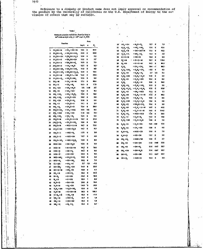
iReference to a co 'mpany. or product name does not imply approval or recommendation ofthe produlct b~y the Universit7 of Califlornia. or thieU.S.Deat nto Eeryt th-x-clusion, 6f others that may b&, suitable. Dprmn fEeg ote x

Medhiol oxdtion me"~h. Reactin iistis incmol..uwccat units, k - AT' explaE*RT)

RateReactionl 0g so' 50 t HO "'P * 0 13.7 0- 1.D

IC~O4 -C,4HM 6 0~51 H, .H6, + 40 136 C 42.5CNOH- M -6,+H - 1.5 $.052 H,O, *M 04 4 OH'+ M 17.1 0 455

CH, 'OH+O, - CH2 OH *H0O 13.6 0 E.. 53- N,0, *H, -HO, *H; 12.2 -0 3.8

3 CH3OH 4ON 4 *.C4OH tH, 0 12.5' 0 2.0 '54 O*H+M .OH+MA 16.0 0 0.0

4CH1OH4 + C HO 2 0 215 oy-M -H.H+M- 14.3, 0 16.0'

6CHOHO -CHOH +O 12.2& 0 2.3, 55 H,4M, -O+H+M, 14.7 0 115.01

I .CH1OH+H CH, +H10 '12.7, 0 s1c14 -'C'.oCH + CH, 19.4 -11 "83'

7 Ck3OH 4CH, -CHOH4CH, 11.3 0 9.8 56 C, H, +CH, -CH,.*CH 4 -0.3 4 8.3

8 CH391I+ NO, -CHOHtHZO3 12.8 0 19.4 59 C3H**+H - 2H& *HS 2.7 '3.5 5.2

9- CHOH 4M -CH 2 04,. M '13A4 6 29.0' 60 'H. +ON N. 4,.Hso 13.3 0' 2.410 CH1H4O1 H1 04H0 12.00 ~60 CH+ C;,4o S .

10 CH 4 0 , - .CH 3+H4MN 17.1 0 6.0 2CH CH+ 360 3.12C4 H C 1 H2 1.'0 1S61 C, +0 -C, H, + O 13A.0 0 5.0

13 CH, 4 PH .CH, tH~O 3.5, 3.06 2.0 641 C2H. +C3 Hj *CaH 4.4Cl H4 17.5 0 35.6'

14 CN,4 +0 CH, 4tON' 13.2 0 6.2 65 csH 4 +0 -CH, 4 CO 130 ,0 1.1

Iii C", 4 NO, .CH 3 +H3?, 13.3 -0 IL0 64 C, H, tM 'C*H, 4 1M 17. 6 0 88.2161 CH, +H NO, CHOO 13.2- 0 0.016~CH4 .,4, 1. .

17 CH + PH .CHO+H, 12.6 0 0.0 68 , CH+ON -CHi*"4 1O 14.0 0, 3.5-1t CH, +0 4CHO*H 14.1 0 2.0 60 C3H 4 0+ CHO,4CN, 1 3.4 0 5.0

it CH, +0, .. CH 8040 1340 26.0 70 C,1H4+M -CH, *H +M 16.6i 0 40.5.

20 CHO4CH3 - CH, *HCO 10.0 0.5 6.0 71 C1H, *M -C 8 H H +M 14.0 0 114.021' CH3 +HCO -.CH *CO 11.5 0.6 0.0- 7JCH40, .HO O 16 0 2.

22 C.n*s + .t CH4 408 12.0 0 0OA 73 C1H + "H C -cH +H, 14.3 0 16.0

22CHO+ M -CH 8 O*H*M 13.7 '0 21.0 74 C1H, 4ON -CH+H,'O i2.8 0 7,024 PH~O*O 01 CH 3O+HO, 12.0 0 6.

25 CH1O#M - NCO 4H 4M 16.7 -0 72.0 7 1 3 O - 3 +H 5506 1.

** ONC 0U2*C 38' 1'26 CHIP4O -HCO*HSO 14.7 0 6.3 76 NCO4O CH+ CO 13.0 -0 4.0

27 CHO4t *.-NCO *H, 12.6 -0 3.8 77 C1H*0 3 HOC 1. .

2s CH1O+o " CO 4OH 13.7 0 4.6 78 CSH*O -CO+CH 13.7 0 0.0

26 CH1O *Hot - CO *HSOS 12.0 0 6.0 76' CH1+0 N.CO t ON 14.0 0 3.7

30 HCO+OH "CO+N;O 14.0 0 0. 0CMO -C*O 13082.

31 HCO*M ..H+CO*M 14.2' 0 19.0 31 cj 4H A CH4H, 11.4 067 25.

32 NCO + -C0414 14.3 0 0.0 82 CH, *ON 4CH*H8 0 11. 0.67 25.7

33- NCO4O# .CO * O -14.0 0- 0.01 8 CH*O, -CO*OH 11.1I 0.67- 2L?7

34 HCO * HOi .CH 8O4O, 14.0 0 3.0 84 C H*, -HCO*O 13.0 0 0.0'

;- -6 *0 -CO*H140 12.5 0 7.0

.6 0*04,- *CO *H 7.1 -1.3 -C-8

:7CO + H0 - COj *OO 14.0 0 23.0

16 C040+M -cO,*M 1. 0 4.1

U1 C03*O *C6+ 01 124 0 43.8

- 40 Il+O, -040H 1430 16.6

41 H, t0 -H*OH 10.3. 1 -6.'

it42 HO0 .. Oa4OH 13.5 .o 16.443 HO4H -Ni*OH -14.0,' 0 20."

44 H20 * 0 4 .HSO+ 40S 13.0 -0 1.8

46 HOiM -1440H*M 16.3 0 105.146 * H0, + NOM 15.2 0 -1.0

It47 4IO,*O -!&H*O, 13.7 0- 1.046 O HO~I 4OH' 14A4 0 1.s4 NO,4I+ *'H, 2 1.4 i 0 0.7-

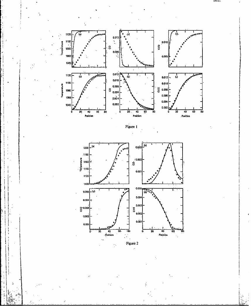
14-11

- ~ .: ~ ;.I.o000000000e0 00b000o~@oo C)

001040 __ __ _ __ _ 'o .

1120 - 0000 0~.01W b 01 c00

1080 0.00006

1060 00o4

0.010

1040 0 0.020. 0080 : osto

1200 00.0 wb 0 .W

1180400

00 60.00

112., 40 so L00 2,, 4 0 80 0 2 0 0 8

120 00011 0.003-000

00

Z03 0.000 .0.

0.002- 0 .002-

0.00 00 0.000 00

I 1!

0.004

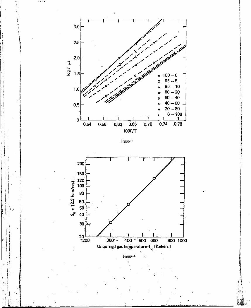
3.0--

0-

i'" '~I- II " . / - I

}' 3.0 - - .'-U

2.0 10 #

01.5

A , X 95-5

./ a- 80-20 ./ /( 060- 40

0.5- A 40-60•20-80

3 0-11000"-

0.54 0.58 0.62 0.66 0.70 0.74 0.78lO00/T

Figure 3

200

1150120'_

100

60-

i .,. 50 .

,640 .-

30

20S200 -300' "- 400 ;;50600 800 1000

Uburnd temperatureT (Kelvin.)

Figure 4

14-13

60 - I Io.---,o _ .. So 44T,-056 -

40

.30 S = 44 P-0 18 1"-oE

20

100.1 1 10

Pressure (atmospheres)

Figure 5,

~46'EU

30

20!0.6 0.8 1.0 1.2 1.4 1.6

Equivalence ratio g

Figure 6

*5 W

1200- 4

1150 2

I 0 24-

/ 20 01

0~ Of

20 20, 40 "60 80

Distnc, cm Distance, cm

,Figure 7-

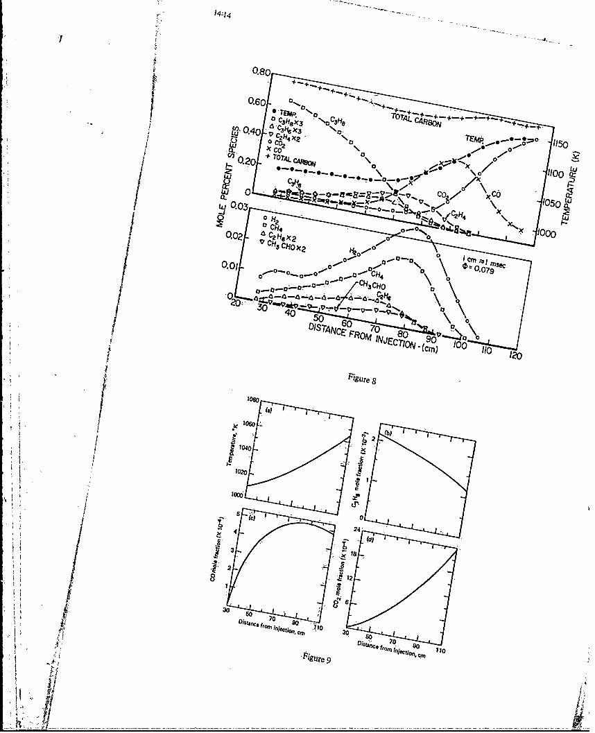
14-14

p-D~-I-fle N ATOA 4S

~'QO 707AL C4 Jsof 0

Lu

II

- 1000

Q0 a10800 10

Ca 3 H 2 t ..

CH

00

02

0010

06

1020

V 'Ct~ foo3

(c)anc 0 rn;~ ~ - 1

4'tr 9 ec4o.

3 (d)18 -

-

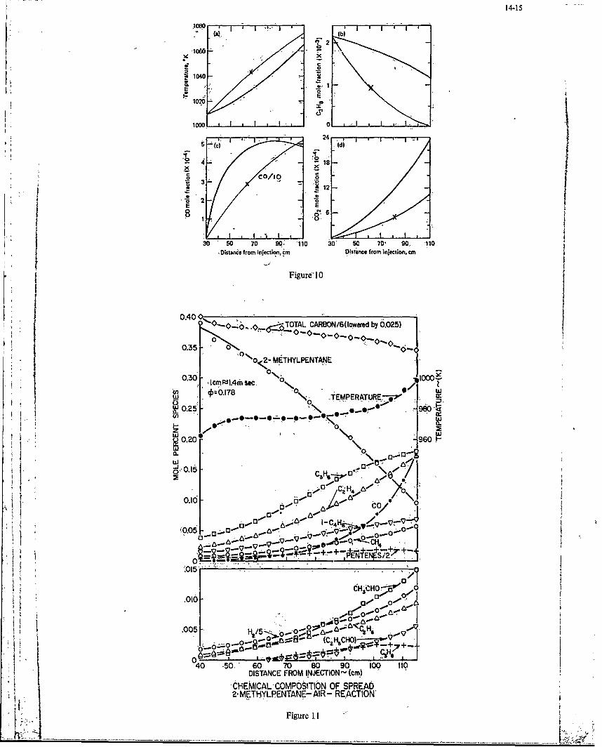
14-15

'1060-

*C

~ 1040

2- E1020

p 1000 on I~0-

5 c) (d)-

C0 -O10C0 3 '~ 2co/io 12 I

40 6. ' -

30 50 70 90; '110 30' 50 70' 90, 10

Distance from Injectionm Dist nce from injection, cmK 0.40 Figure] 0 ~ 605

03 TTAL CARB0N/6Ioweredby0250 0'-_0 0 _p 0 ,

2METHYLPENTANE4

0.30 "N 00

0--0.178 JEMPERATURE~

0

0.20 \10

a...

010 *

C3HG

0.- J-C 4 _6

13O

(C HCH0)-O- 13 00 * eel

00 -5 60 738 0 100 ,10,DISTNCE ROM NJECI0N0(cm

.C0EICA COM11IIO _OF SPRADCZ2ME~hYLPNTANE- I NECION'

Figur 1.+___ __

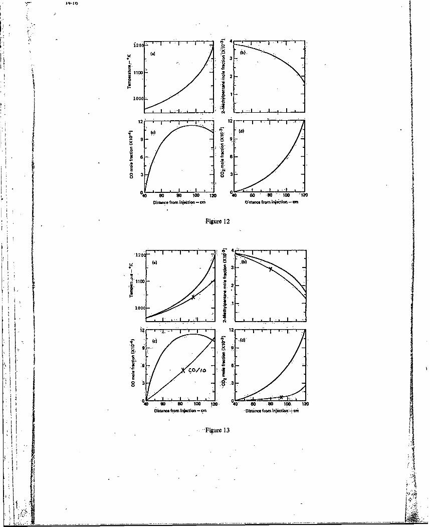
1-200- ,- :

*3-

E

-1000- -

I i -

(C) (d)

6---

3 3

00

60 so 100 120 40 60 -8010 1120I Distnce from injectbn - cmn 0 stance from injection - a

K J Figure 12

120'c-

l~1wI~ -

,t 11000-12 . 12L.L..

0 A, 0I 0 .. '

s60 so 108;0,o s 100 1206 istance from injecian - cm istance from injection--, cm

-Figure 13

K 14-17

DISCUSSION

Comment by N.Peters, Ge

You point6d out that glbbal modelsuch as the 9ne of Dryer and Glassman can-not describe processes where the

initial'kinetic steps are impoiiant. However, there are very old proposals, of two step models, -for instance, that ofZeldovich -(A + B - 2B, 2B -* C), tI.at concentrate on the initial kinetics. In this m6delthe intermediate speciesmay be interpeted as a radical that catalyses the fuel consumption. In his recent thesis, W.Hocks- calculated the

fuel consumption during wall 4uenchiig by elementary methanol kinetics and by Zeld Aih's two step kinetics. Theglobal model did a good job in this case,.

1. Hocks, W. PhD-Thesl5 - Institutffir Allgemeine Mechanik, RWTH Aachen, Germany.

fik1R&

ii- I

I

1--C __ |

PCaesece/Disperiion flodelling -of*Gas Turbine Comiiustors

David-T. Pratt,,Professor-and6Chairmanbeparbtment of Mechanical Engineering and- Appliid'Aechanics

-The2Univerity-of Michigan

Anti Arbor, Michigan 48109USA

Mellbr'hag shown :that t- ,4he turbul entmixing time, is 'the mostdominant single-'characteristic time over -the'entire-range of present orAdvanced con~cept combustors, and over the full load ranige from idle to full,-aswerl. as norkuntely, classical feactor-theoretic or "miodular" models,-aswel asfinlte-differenceapprxiniate solutions to the-governing

differential ejiations,-have heretofore regarded isl as either zero orinfinite. Stochatic or'Mone Carlo -methods hiqe shown promise. for includ-ing effects of 't5s>O, but only for simple, chemistry. Preliminary-experiencewiith a-newly-;developed- algorithm for integration of batch- reaction-chemicalrate-equatlons shows great,-promise in-makingtractable the corbinedmodelling-of botk-flnite-ratie nicromixing and complex, finite-rate chemistry, whichis -necessary for modelling~of pollutant -formation- and -combustor stabil'ity.

1. CHARIACTERIZATION OF COMBUSTOR PROCESSES

A. M. Mellor'has usefully characterized the, complex interaction of-serial and competing-processes ofchemistry, heat, -mass-anti momentum transfer-within a 'gas tpurbjne, combustbr in-terms of "characteristictimes" (or reciprocal frequencies) 6tf-the dominant-processes.l1) These Are summarized in-Table 1.

(All tables and figures appear at'the'end-ofthe paoer.)In~designlng -new~combustors, or analysing or -modifying- existing. combustors for: improvpd efficiency,

wider turndown ratio or stability limits, reducedp -pollutant production, or improved 'patternl'actor, it isconceivable that-any of the processes rep~resented iin Table I could becomd-the dominant or conti~blling step.For examl hg-altitude flameouft'or extinction is thought t 'be doe- to Thc controlling At lowpressures.()

!g)

in-conventional -combustors, 'Teb ca In.usually be,,removed from controlling- status.sby improved- vaporiza-

imotatin onrllfj-plltfi mison'-bt it,-isnegligible forpressure atomization.-I ) --

M61 ir- ha- shon st"a the 'turbulent mixing time-, I§s the most dominant single~ characteristic 'tira&,overthehti6,rfig ifpresent or1kdvanced concept combustors, and over the-full--oad range from idl--to

fulLi~werIn'6ther words,' 'at the,-cditions' ty'pical of gas turbine--operation, chemical and heat- release*atfe-alwakys -strongly--influenced-by,- and fri~uentlyt ontrol Ied by', the rate-of turbulent- mixinrg of

a) vporiedfuel'-with air, $b) rdruae'undg, e,,'hr~tnsi~h prim~ry zone, or

c) dilution air-with priduct' in', h ,,s-e-ondlary zon6eI'3)

Historically, gas turbine combustor, devlopme~nt, has been' principally, a,:ei al and-errorpr'ocess. Afterthirty. years 0f c,.mutie ypine, caiutio'us, incremental' imprqve'ments -in'ecobu stor design( 4) are-possible. Uhiki~compressors and turbines, in whc,,e~yaic.ad-tut a vibrations are to sorfie

the need tomiidify or 6design-combustors for-.reduced imokb&e ad~aseouspoollutint formation - always-while

maintaining-or improving- combustion efficiency, tu~ndow'r6tio and pattern faftoir - has' created a need -forU Ibetter understandingof the sujbtle, interaction of 'th~selcoupled fion-j'Inear processes.

The concurrent, advent-of the-digital1 corapute-rdhas rais'e - the -hope ttlkAt more sophisticated analyticalmodelling might- -eIad to reduced --expendi tures of'time and manpov'er in achlbving ia4roved-designs. While'this promise. hits-by no-means been fully realized, -tkebe are som'exencouragi'nq signs.-'* -For example, thepresent development~of preVaporized, preiiixed combustors '.or l'w,Illutaht forrnation) originated, fromnumerical' parametric-studies-which sh 6d that there should existairowinoofuearrt,temperature and residence time within which stable, efficient combust~oncould-be achieved, with lowNO ,CO and UHC as-well. 5)x

Generally-speaking, modelling --fforts to-date--stem from one of two fun Amentally distinct Approaches:

a) Thoseobsed on chemidCal reactdr-theoretic or-"pop~ulation balan?" models - sometimescalledthe, !mddular' 'approach --in which the-fluid medhankhs ard~simolifie&--to theexten't that conveictive -flow and tu~rbulent 'mixinig is- riprese'nted'.by'interconnected Well-or perfectly-stifred rei6fo § (PS11's')',and-plu§ flow reco

-b)- The second approach- is to solve'the-finit6-difference approximated differ'ential- e~uationsfor-consdrvation-,of-mass, species, momientumand energy, usually simplifyiitecmsrto the,point where pollutant formation processes cannot,,be adequately reprelented.

7)

What both of these approaches have lacked to date is the ability to model the effects qf Tsl, thiemost universally important characteristic time within- the combustor. -In the modular apprah trsl iS,by definition, equal to zero in PSR's, and is zero for cross-stream mixing and infinite for age mixing(axial diffusion) in PFR's. In vigof these-inherent restrictions-on PSR's and PFR's, Swithenbank' s

attnptto ccont for fiite'rs~ ~~ 5 simply, equivalent to ih reasing the Value of 'rhc,whc tlremains a-homogeneous reaction time. :.Predictions~resulting from tnis simpiitication may be-useful foetrend analysis, but canntbe valid: or quantitative prediction of pollutant formation and destruction, asthe effects of inhomogeneity orsegregation(3) are still.-not represen'ted.

Infinite-difference modelling, it has been-necessary-heretofore to-treat turbulent exchalnge processesas quasi-laminar; that is, to Assume that, within a compUtdtional cell, local molecular homogeneity exists,-or T 1 = 0. Some attempts have been made to include moment equations for the probability density function(PDFJ of a -passive scalArmixture fraction(7),,which-accounts for the effects of finite- V- but only withthe "flame-sh-eet"'assumftion that -T = 0 Thus bothapproaches tordate-faii ;As-quaniitaiively correctmodels for pollutant- production, behuse'both Thcand-Tsl are'known to play,,essentiil roles.

In an actual combustori recirculating flow is necessary for flame stabilization, while plug or streamflow is required to ,move-the working-fluid from compresso r to-combustor,to allow comnbustion reactions toprogress towards completion within-th6 comnbustor, and to-moVe ,the-working fluid from the-combustor to theturbine inlet. A-PSR is- an- idealization of a-region with sirong'-convective -recirculatibn, whereas a PFRis an idealization of a simple stream tube flow. Due-to recent advances in computation of'stochastic or"Monte Carlo" -methods (3,8), together with improved'algorithms for calculating equilibrium and non-

, "silibriun chemistry-0(,lli,it is now possible- to:-introduce finite-rate microrilxing into both the PSR(age mixing) and PFR- (cross.-sxream mixing only) models. 'In the PSR, this improveme~nt allows assessm~ent ofthe effects of primary-zone inhomogeneities-due -to-fuel-air ratio,. temperaturei and"age"', or degree ofreactedness within fluid elements. In the PFR regions, finite-rate mixing of secondary air admission intothe Post-primary stream~may be described, leading eventually to prediction of mixing inhomogeneities. onpattern factors,

3., THE COALESCENCE/DISPERSION (C/D) MODEL

A simple Bragg combustor model-,is--asslumed ior presentpourposes: An imperfectly-stirred- reactorrepresents the-primary zone, followed by aplug-;flowregion.

-The- primary zone contents are discretized into computational cells or "turbules", which may bej regarded conceptually--(but not literally ) as primitive-representations of single-scale-turbulent eddies.

The mass flow rate through the-primary zone -s then-represented-by a number flow rate of turbules -given by

rN/<p>V = Nitr ; 'r, i~> 1

where- <p> is the ensemble mass density in the primary -zone, V is the volume, ; the mass flow rate, N isI the-numberof turbules-nAt -c is-the mean-residence tjme' in-theprlmary zone.

I Micromnixing,- or mixing between -turbul]ant- eddies ai_--thmicro-scale level, Is. simulated'by considera-_-ton Of C sin's tlime constant' .for'decay-of a-concentration fluctyation in an 'isoteopil. tyrb~leynt

- ~field, O.? -Defining 'I -as the~ratio--of mixing frequec ( th feed wit-esu c"alsence andpir~o-turbules within the reacTor- are allowed to-simply averag 'e- rrpr~i wiher.suh1caesec n

diesion" pair 'interaction 'ildwid-,per -time interval '(-/I, -N), Pairs- are chosen by random -ilaction sothat there 'is-no bias with respect to- turbule- age, thus -rep,.,esentin§, a weill-!stirred- reactorlth 'non-zerosegregation.(3) During the time interval between C/D'events, all turbules undergo adiabatic batch reaction,I- using either an infinite rate (equilibrium) assumption or achemical kinetic mechanism and rate data, asdesired. Whenever'-a feed-timne-interval-(-TIM) has,-elapsd-iohe-turbule is'selected-at-random to be removed'rom thiseml- and..isreplacedcby a-frish-f~f-urbule.

The assembly-'of turbule , 4s --lnitialized -by ~assuning~a-homogeneous-PSR.I~distribution of mole numbers andcorresponding- tnprtuP Th-C/D s~fiulation ii-allowe'd to-.run for thi.- to fivd equivalent residence-times, until -.the ensen'b4e- tatistis - .banv:And, variance of properties-) are 6bseir('ed to stabilize. Each

turble s ten-ll eoA irdrgofuiP'-or'batdh- 're~tio-for-thd& e~ojdary zone'-residence -time; no furthermixlng~is- csijre-To "in e -)del in'the~preni s'tate -of development. Finally', ensembl 6,averagesare obtained to irep'e'nt, the oar p".;- iesat- cob~ it. -Mean-and standard deviation (rms A values

jare ofta-.4,; th .fq . -6mble a t-r-e mul , 1m tr oment dquations- of desdripti~dK f statist, ., fct -exqsrp~e fJ-- Tpe

1 N (2)U andi -<T> -=~X

1 M - 2 (3)r Ns (Ti V T) 2

-4. SUMMARY OF COMPUTATIONAL, METHODS,For finite-rate gaseous chemistry, either premixed or non-premixed, it was found necssary to develop

a new algorithm ,1for ihtegration-of -th~e coupled, non-liiiear, first-;order ordinary-differential equationsdescribing the, variation fih comoositidn and temperatur6 iwith,-elapsed-time within a constant-pressure,--adiabatic bAtchi1reactor (turbule). The rdquired-,characteristics -for this algorithm'were:

(A) Spegd. The large number of species (15730) and turbules (presently 20, eventually-up, to --

~50OFtequires the-fastest possible- -peed-of execution.

)Stabili ty. Te infinity ofinitial conditionsieuivalence ratioand, chemical time scales

resulting from rahdom selectin procedures ,requires -an extremely robust. algorithm, preferably

with automatic stepsize variation.

(c) Accuracy. This .is relatively unimportant, consistent with the crude assumptions on which theentire scheme s prediated. Further, Acc'ulated~bundoff errors leading to violation of aton

conservation tend to be "flushed away" by the replacement of 6utflowing,-turbules with the steadyiiflow of reactants of prescribed'stoichiometry.

An algorithm was developed~which.meetsall-,of the above criteria, and is~describedmin detail in

Reference (11).

Briefly, consider the set of species- conservation equations for transient batch reaction,

dt -ri. , i = 1, NS

where {ai represents'(i= , N S)gas phase mole numbers, where ri is the mass-specific rate of disappearanceof ith species, as given~by

ri '- (& -c- T)(R -Rj) i=I,NS- (5)

j=l

where pis the mixture gas density P=P/RTom , a ii the sum of all mole numbers and Where R and R., theforward and revese'rates of "he j-t reaction (i = 1:00J, are given by a~modified Arrhenius expression

B. N. U.NS 1R =IOJT 3exp (-T ./T)(pOm) JI (Pk) " (6)

k-l

and

B.N. NS (7)R. =10 "T exp(;4T /T)(p6 ),J HI ((7)'x

. M _,, I Pk=l

Following Liniger and Willoughby (12 ), the solution to Eq. (4) oer the short time interval h is firstapproximatedby a "tunable trapezoid", n t E

oi - h l-Wi)r i +Wr*], i = 1, !S (8)

where the "tuhing" or integrating factor -W- is to be determined by "ekponential-fitting" of ri over'theA ih ; iV h; 'as oll ows

If .ri should vary exponentially with time over h, so,,also wouldo 1i as it is the integral of-ri;therefore

do . (9)

Brardon (13). defines a diagonal transition matrix Zi. for the eigenvalue ci over the integration intervalk h so,that Eq. (9)-is givenby

do. zdt -ri = G-- i 0)

'With the substitution of Eq. (10) into Eq. (8), algebraic manipulation leads to the identity

Wi = Z Z1 11'(e, -)

If ri should actually varyexponentially over h, then Z, is given precisely by Eq. (7). However, for

arbitrary, non-exponential variation of ri, Brandon-(3) suggests °napproximation to Zi overthe interval

h,,as followst

=. h 'i . [(!ri rk)(0) - ] (12)

where the supersc lpts (o) and (s) refer to-values evaluated at the zero-th-and current-(or last) iteration

duringconvergence of Eqs. (8).

In the present application, a Nevoon-R,iphso6 functional was defined for convergence of Eqs. (8),

f - i1T3I + .W ri + ri I , NS (13)

15-4

Following Gordon and McBride (14), a wise choice of correction variablcs for solving Eq. (13) arethe natural logarithms of the US mole numbers (ai ,i=l,NS); of the sum of the nole numbers,

NS

am -0 ok ; (14)

k= 1

and of the temperature T.

The Newton-Raphson correction equation for Eq. (13) may now be written asN af fi

N log A loga a oE a log k + a A log mk--1 (15)

afi

+ af l A log T = "fis i = I,NS.

Noting that the integrating factors W. are considered constant during each iteration, partial derivativesof the species -i functional fi of Eq. (13) are

af i i k + (aJJa ( j ~ -= - )hi-R1 i 1, NS (16)a log ak - 1w) + ( j*i) jakj i lkj '

j=l

0 fi =k I J =J

af ~ 1a log Om 2 : (a, - ajj)(R_ n-Rj nj)+ r (17)j=l

andafi JJ

a og T p I( i a [Rj 13 1TL[-F{Nj--l

-R~ {N +T n'.' + ri (18)T

The functional for reciprocal mixture mole number, a,, is simply

NSf. I- a Ok -m (19)

and the corresponding correction equation i

NS MSkAlogak'amAlo-m m mk (20)

k=l k=,l

The functional for temperature is the equation for conservation of thermal energy for adiabaticbatch reaction,

NS

f , S (2))T T -oR-

and the corresponding correction equation

ICIiS hkok NS

p Aloga + o i.Alog T

k=l i=l (22)

NS h NS h*

, k i=l

The partial derivatives-required in Eq. (12) for the approximated diagonal transition matrixelements Zi are given by

;o(ri. - i (R -R-jkj (23)

Tak 'k 2 log ak (P~k) ~= ~ 3 Jj=1 '

which may be seen to be related to the second term on the RHS of Eq. (16).

In order to preserve the absolute A - stability of the implicit formulation (15) and to avoidnumerical singularities, the integrating factors of Eq. (11) are actually calculated in the code as

0.,5 , Zi < 0.015

I I Zi > 0.015 (24)

Z i (e Zi - )

The evaluation of the Jacobian for Eqs. (13) i2 done analytically, following the efficient codingtechniques of CREK (9)_ As the Jacobian elements als" contain the expressions required for evaluation fthe integrating 'dctors Wi (which are regarded as constants during each iteration) both accuracy andefficient computation are achieved.

Limited experience to date with the new algorithmhas shown it to be remarkably stable and accurate.ror all practical purposes, the limiting factor in its use appears to resolution, rather than stabilitvor accuracy. Of course, execution time is directly proportional to the desired resolution, independentof other considerations.

Stability is insu rd %"iply by using a modified version of the same "self-adjusting" underrelaxationparameter used in CREK.( , ,u This technique, originally due to Gordon and McBride (14), calculatesunderrelaxation parameters designed to assure that, for any iteration,

i) Major species (mole fraction > 10-8) may not increase by more than a factor exp(2).

ii) Minor species (mole fraction < 1O"8 ) may not increase so as to exceed 10-4 mole fraction.

In the present application, underrelaxation parameters so determined are applied not to the molenumber and temperature Nevton-Raphson corrections at c Fixed step size, but rather to theTime step sizeh itself.

In practice, the above criteria insure stability, but oi not insure adequate resolution. Therefore,An additional constraint was added:

iii) The temperature may not change by more than 200C.

With this additional constraint, automatic stepsize control was easily achieved, and resulted inbetween 2 and 5 iterations per time step on the test problems ccnsidered thus far.

5. APPLICATIONS. I: COMBUSTION OF PREMIXED HYDROGEN AND AIR IN A JET-STIRRED REACTOR

A Longwell jet-stirred reactor, such as that described in Reference (16), and shown in Figure 1, maybe thought of as an idealization of a highly loaded gas turbine premixed, prevaporized combustor primdtyzone. For this reactor he mixing parameter may be estimated to be about Im = 10, with Im

= 50 being apractical uppi, bound.(17pb

The effects of temperature and mole number segregation due to degree of reactedness are demonstratedin th's first attempt to include finite-rate chemical kinetics with complex chemihtry, using the simpln iedmechanism'-for H2/air combustion given in Table II.

The simulationwas run for five mean residence times, a sufficient time fcr the ensemble statisticsto stabilize. The effect of segregation on ensemble-mean reaction rates can be characterizedby a "contact"index" (3) X. for an individual reaction, def'ned s the ratio of ensemble-mean reaction rate to theapparent irat based on ensemble-mean properties:

X 1 r'r. {<.i: T7" i - ,NS (25)

The calculated values of contact index for each forward and reverse reaction are given in Table II.Also-shown are the ensemble mean and rms values of temperature, <T> and T , as calculated by Eqs. (2)and (3). As would be expected, the reactions with highest activation temF' atures T. (and therefore thosemost sensitive to temperature) show the greatest deviation of X from unity.

6. APPLICATIONS - II: PREMIXED,'PREVAPORIZED COMBUSTION IN A SWIRL-CAN COMBUSTOR

The purpose of this investigation was to assess the applicability of C/D modelling in predictingpnllutant formation in gas turbine combustion. This combustor was selected for C/D modelling sincemeasured emission index data are available (18), and the additional complications of fuel spray evaporationare not presenii in premixed, prevaporized'combustors.

A simplified model of an array of swirl-can modules "Figure 2) was developed (19), with the followingassumptions:

15-6

(1) Upon entry to the combustor primary zone, the fuel is completely vaporized and thoroughlymixed with the primary air.

(2) The conbustor may be represented as a modified Bragg combustor (2) as shown in Figure 3.

(3) A 17-step mechanism for CO and H2 oxidation and NOx forration due to Waldman (20),

together with a global pyrolysis step, C12H23 + 02 - CO + H2 , of Edelman (21) is used,as shown in Table IV.

The combustion chamber was represented by a zone-type model, shown schematically in Figure 3. Thesizing and location of PSR (perfectly-stirred reactor) and PFR (plug-flow reactor) elements was doneby inspection from Figure 2.

The primary zone was modeled in'two different ways, first as a homogeneous (fully micromixed) PSRwith zero segregation (Tc£ = 0), using the complex kinetics code CREK (9, 10), and secondly as a partiallysegregated WSR (well-stirred reactor), with effects of segregation modeled by the C/DO model with I = 2.0assumed. The secondary zone was treated identically in both cases as simple PFR batch reaction of"theeffluent gases from the primary zone without further mixing (Tst + =I m = 0). Test conditions for thecalculations are given in Table V.

In Figures 4 and 5, comparative results if mea ;ured and predicted values of emission index valuesfor NOx and for CO, respectively, are presented.

IXIn Figure 4, it may be seen first that the premixed, prevaporized concept results in considerable

reduction ..f NOx below the equilibrium values. The predicted values for assumed homogeneous (t = 0)PSR primary zone ;hows the correct order of magnitude but a "peaky" trend that differs consideragly frommeasured values. A single computation using the C/D model with I = 2, and the same conditions, at(F/A) = 0.03, shows far better agreement with the data than does The homogeneous (Im * O; TsX = 0) PSRprediction.

In Figure 5, the CO emission index values predicted by the homogeneous PSR model are seen toapproximite' very closely the equilibrium values as (F/A) approaches stoichiometric; at fuel-leanconditions, the effect of Th is seen in the upward trend of COEI. The single point represents the COEIpredicted by the C/D model with m 2, at (F/A) = 0.03. As with the NOEl in Fig. 4, the "smearing"effect of segregation or inhomogeneity is seen to give better agreement with the data.7. DISCUSSION AND CONCLUSIONS

Needless to say, a single point comparison of computation with the C/D model with the NASA datais insufficient grounds for drawing strong conclusions. However, compared with a conventional modular,homogeneous (I -, -) PSR-Pt:R Bragg model, the (C/D)Bragg model with Im = 2 is seen to imorove thecomparison with data at very fu,.l-lean conditions, for both CO ind NO emission indexes. Theseresults are at least encouragi ,g. Of more significance is the fdct that the computation is feasibleat all.

The preliminary results reported are therefore encouraging for the use of coalescence/dispersionmodelling for prediction of pollutant formation and eventually flame stabilization in high-intensitycontinuous combustors. Extensions of the concept to flows lacking the strong convective recirculationcharacteristic of the present system are possible (3), and such work is presently in progress.

An additional benefit of C/D modelling that has not been explored here is the potential ability topredict realistic combustor stability or blowout maps, as wel, as transient behavior. However, thevariation of IM with combustion temperature during transient; would have to be calculated. 22)

. REFERENCES

1. Mellor, A.M., Gas Turbine Engine Pollution, in Progres in Energy and Combustion Science, Vol. 1,N.A. Chigier, Ed., Pergamon Press,.1976.

2. Bragg, S.L. and Holliday, J.B.: The Influence of,Altitude Operating Conditions on Combustion

Chamber Desijn, in Selectdd.Combustioh Problems, II, M.W. Thring, Ed., Butterworths ScientificPublications, 1956.

3. Pratt, D.T., Mixing and Chemical.-Reaction in Continuous Combustion, Progress in Energy andCombustion Science, Vol. 1, N.A. Chigier, Ed. , Pergamon'Press, 1976.

4. Hazard, H. R., Combustor Design; in Sawyer's Gas Turbine Engineering Handbook, Vol. I, J. W.Sawyer, Ed., Gas Turbine Publications, Inc., 1972. i

5. Wade, W.R., Shea, P.1., Owens, C.W. and McLean, A.F., Low Emissions Combustion for the Regenerative11 Gas Turbine, Part 1: Thdretical ahdDesgn Considerations, ASME Paper No. 73-GT-ll, 1973.

6. Swithenbank, J., Tiran, A. and Felton, P.G., Fundamental Modelling of Mixing,Evaporation and Kinetics

7. Elghobashi, S., Studies in the Prediction of Turbulent Diffusion Flames, Studies in ConvectionVol.. 2, B.E. .Launder, Ed., Adadeni&,Pess, 1977.

8. Flagan, R.C. and Appleton, J.P., Combustion Flame 23, p. 249i 1974.

f 9. Pratt, D.T. and Wormeck, .J.J.: CREK A Computer Program for Calculation of Combustion ReactionEquilibrium and Kinetics in Laminar or Turbdent Flows' Report WSU-TEL-76-1, Washington StateUmIversity, 1976.

15-7

10. Pratt, D.T.: Calculation of Chemically Reacting Flows with Complex Chemistry, in ktudies in Convec-tion-Vol.II, Academic Press, 1976.

11. Pratt, D.T., New Computational Algorithms for Chemical Equilibrium and Kinetics, 10th Macerial

Research posium, National Bureau of Standards, 1979.

12. Liniger,-W. and Willoughby, R;A.: Efficient Numerical Integration of Stiff Systems of OrdinaryDifferential Equacions, IBM, Research Report RL-1970 (1967)i

13. Brandon, D.M. Jr.: A New Single-step Implicit Integration Algorithm with A-Stability and Improved

Accuracy, Simulation, 17-29, July 1974.

14. Gordon, S. and McBride, B.: Computer Program for Calculation of Complex Chemical Equilibrium Compo-sions, NASA SP-273 (1971),-

15. Lapidus, L. and Seinfeld, J.H.: Numerical Solution of Ordinary Differential Equations, AcademicPress (1971).

16. Malte, P.C. and Pratt, D.T., Combustion Science Technology 9, p. 221, 1974.

17. Evangelista, J.J., Shinnar, R. and Katz, S., Twelfth Symposium (International) on Combustion, p.401, The Combustion Institute, 1969.

18. Niedzwiecl.i, R.W. and Jones, R.E.: Pollution Measurements of a Swirl Can Combustor, NASA TM S-63160,1972.

19. Brewster, M.Q. and Pratt, D.T., Modelling of Pollutant Production in a NASA Swirl-Can Combustor,

Western States Section/The+CombuSlohn Ifistit6te Paper No. WSS/CI '78-38, 10'8.

20. Waldman, C.H., Wilson, R.O., Jr., and Maloney, K.L.: Kinetic Mechanisms of Methane-Air Combustionwith Pollutant Formation, Environmental Protection-Technology' Series EPA-560/2-74-045, 1974.

21. Edelman, R.B., Fortune, 0. and Weilerstein, G.: Some Observations on Flows Described by CoupledMixing and Kinetics, Emissions from Continuous Combustion Systems, Plenum Press, 1972.

22. Riley, J.j. and Pratt, D.T., A Proposed Hybrid Technique for the Simulation of Mix .,g with ChemicalReaction, [echnical Memorandum No. 146, Flow Research Company, Kent, Washington, rio',ember (1977).

8. ACKNOWLEDGEMENTS

This work was-supported in part by the National Science Foundation, Grant No.,ENG-7684533, by theKistler Glass Research: Fund of the UnivE,-sity of Utah and by the AVCO-Lycoming Corporation, Stratford,Connecticut, and has been reported previously at the Project SQUID Workshop on Gas Turbine Combustion,Purdue University, May 31-June 1, 1970.

Patti L. Case provided valuable technical assistance during the development of the computationalalgorithm.

9. TABLES AND FIGURES

Table I

Mellor's "Characteristic Times" for Combustion and PollutantFormation in Two-phase Turbulent Combustion (Ref.1)

Time Symbol Physical or Chemical Process1>+ Fuel droplet lieftime T eb Droolet evaporation nd/orcombustion

Eddy dissipation time Small-scale turbulent mixingfor injected fuel fi ner the fuel injector in the

recirculation zone

Eddy dissipation time T sl Large-scale turbulent mixingin. the shear layer between fresh air and the re-

circulating burned gas-fuelmixture

Fuel ignition delay Th Homogeneous combustion of theand burning time fuel to CO2

No formation time 'no Homogeneous kinetics for NONo frmaion imeTno formation

__ __ __ __ __ __......_ __ __ __ _ __ __ __ __ __ _

15-8

TABLE Il

Conditions for C/D Simulation 6f Mixing Limited Combustionof Premixed Hydrogen and Air in a Jet-stirred Reactor

Fuel: Gaseous H 2 at 300 K

Oxidi zer: Air at 300, K

Fuel-air Ratio: Overall fuel-air equivalenceratio =O.5 (fuel lean)

Reactor Pressure: lOO0 kPa (1 bar)jReactor Loading: 500 kg m3bar- -2 1

Residence Time: Ca. 5 ins.

TABLE III. Mechanism, Activation Temperatures and Calculate~d

Contact indexes for Mixing Limited Combustion of Premixed

Hydrogen and Air in .a Jet-Stirred Reactor. P - 1 bar, Im z 10,

0.5, inlet T.- 300K; <T> =1112K, T RMS *2520C; T EQ z1643K.

Reaction, Tf/Tb XfX

1. H + 00 OH 16.5 1.34 220.5 0.9

2. H 2+ 0 4H + O H 9.4 0.5K j 27.3 1.113. H0+0 O +OH18.1 2.1

H201.0 1.1

4. H + H120 . H2 + OH 19.9 2.0t4.8 0.55. N+04 O+06.3 1.02+:N + 41.4 7.1

1 . 2 0~-N . N 75,5 64,66 N2+0'N+NO0.3 1.1

V7. NO + M 4' N + 0 + M 149.0 13,840.01' 1-6.1 0.9V I8. H + H + M '+ Hq + M 10.3 1.1

101.38.6~1 I9. 0O+ b+ M '4 +H 0.3 1.0

2115.5 894.1

10. H +, OH +,M -H 2 0 N 0.0 0.8111.2 1,059. 0

11. H 2 4 0 2 + OH + OH 43.0 1.625.0 3.4

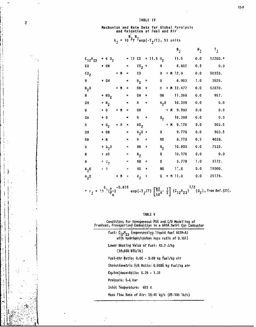
15-9

TABLE IV

Mechanism and Rate Data for Global Pyrolysisand Oxidation of Fuel and Air

B. Nkj 10 IT jexp(-T./T), SI units

B. N. T.

C 12H23 + 6 02 = 12 CO + 11.5 H2 11.5 0.0 12200.*

CO + OH = CO2 + H 6.602 0.5 0.0

CO2 + M = CO 0 + M 12.0 0.0 50353.

H + OH = H2 + 0 6.903 1.0 3525.

H20 + M = OH + H + M 12.477 0.0 52870.

H + HO2 - OH + OH 11.398 0.0 957.

OH + H2 = H + H20 10.398 0.0 0.0

H + 0 + M OH + M 9.903 0.0 0.0

OH + 0 = H + 02 10.398 0.0 0.0

11 + 0. + M = HO2 + M 9.176 0.0 503.5

OH + OH = H20 + 0 9.778 0.0 503.5

OH + N= H + NO 8.778 0.5 4028.

H + ,N20 = OH + H2 10.903 0.0 7533.

N + No N2 0 10.176 0.0 0.0

N + C, NO + 0 6.778 1.0 3172.

N20 .q, NO + NO 1>0.,0 0.0 15000.

N 20 + M N 2 + '0 + M 11.0 0.0 25176.

B 0.815* [ .) 9T 1/2r in exp ( T. (C12 H 23 ) from Ref.(21).

TABLE V

Conditions for Homogeneous PSR andC/D Modelling ofPrsmixed, Previorized'Combustion in-a NASASwii1 Can Combustor

Fuel: C 3 rees ntingliquid fuel ASTM-Al

with hydr6gen/carbon mass ratib of 0.161)

Lower Heating Vaiue'of Fuel: 43.3 J/kg

(18,600:BTU/lb)

Fuel Air-Ratio: 0;02 - 0.09 kg fuel/kg air

Stoichiometric .F/A Rati6: O.'0685 kg fuel/kg air

tquiValintetRi; io: 0.29 - 1.31

PreSsure: 5-6 bar

InM l Re0ipeateAir: 3613 K

j Mass Flow Rate of Air: 38,-45 'kg/s (85-100 lb/s)

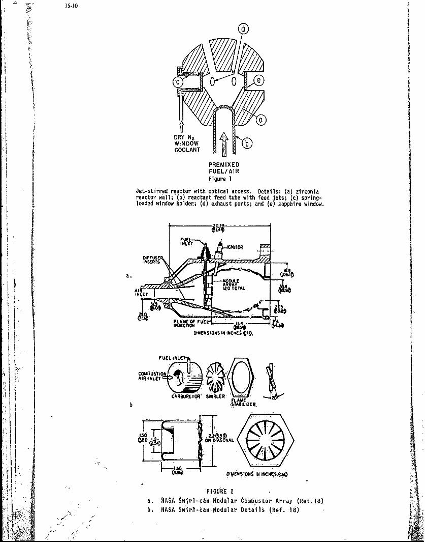
4. 15-10

d j1CI

f PREMIXEDJ FUEL/AIR

Figure 1

Jet-stirred reactor with optical access. Details: (a),zirconiareactor wiall;'(b) reactant feed tube with feed jets; (c) spring-loaded window holder; (d) exhaust ports; and (e) sapphire window.

406-IIa.

AINLET

P~~IE 1 ~ MNION S IN INCj C1 ES).M

CARBRET'FIGRE 2'

b. 4AS Swr-an d lar eal Ref,8

A.5 T2.0 6 SA

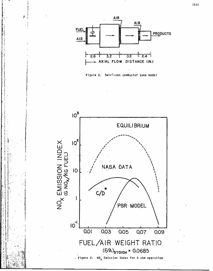
15-11

AIR

PROD UCTS

1 2.6 1 3. 2 3.2 I;' .2AXIAL FLOW DISTANCE (IN.)

31Figure 3. Swirl-can combustor zone mode',

EQUILI BRIUM

zJ

ZI /_ NASA :DATA

0 PSR MODE

FUL/I WEIGH RATIO

Y (F/A)STICH " 0.0685L ~~:Figure 4. NO Emission Index for 6 atm operation-

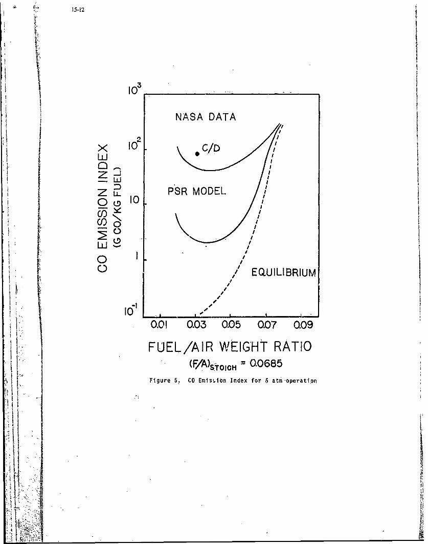
15-12

103

NASA DATA

L

z U PSR MODEL

0 10

-t -

~10.01 0.03 0.05 0.07 0.09

FUEL/AIR WEIGHT RATIO*iI(F/A)sToQH = 0.0685IiFigure 5. CO Emls~.ibn Index for 6 atm-operation

15.13

DISCUSSION!

W.P.Jones, UKYou showed a graph with some measurements from the NASA ,ombustor and one prediction with your coalescence/dispersion model. In a log-scale, I have difficulties to assess the level of agreement. Could you tell us what theactual numbers were?

Author's ReplyYes,,it was a log-scale, and the right numbers are on the scale (see Figure 4). Comparing the data we found oneorder.of magnitude difference (a factor of 2 or 3). I don't think it's terribly important. The conclusion stated inthe paper is that it was going in the gobd direction.

'I

fI

I ':

IC

Sis

til

16-I

MOVELISATION VE ZONES DE comBUsTTO EN R~EGIME INSTATIONNAIRE

par Francis HIRSIGER et H616ne TICHTINSKYOffice National d'Etudes et de Recherches A~rospatiales (ONERA)

92320 Chatillon (France)

Les difffirents types de zones de combustion susceptibles d'atre itudiges et mod61is~es prdsen-tent un certain nombre de caractares conmmuns ;elles sont le siage d16coulements assez complexes, eng~ngral -tridimenojonnels, comportant souvenit des zones de recirculation et des zones d'injection lo-calis~.es. Par aillours, lea phfinomanes de combustion prdsentent'un aspect instationnaire qu'il eat im-portart de mettre en Evidence et de reprdsenter. La simulation numfirique devrait en outre compldter lea6tudps exp~rimentales difficiles A mener, plus particuliarement dans lea rdgimes transitoires.

Une modglisation des 6coulements lea plus simples, prdsencant cependant simultanfiment ces diverscaractares, a 6t6 entreprise af in de ddgager des comportementa caractdristijuea plut8t que de tenter derepr~senter l'enaemble des ph~nomanes intervenant dana des zones de combustion rdelles, g~omdtriquementcompliqudes. La technique de moddlisation conaiste A 6crire lea Equationa de bilans instationnaires del'a~rothermochimie, tenant compte de la dynamique des gaz de la diffuision laminaire turbulente et de lacinfitique chimique, pour un ensemble de cellules reprdsentant le domaine a Etudier, Ces Equations de bi-lan sont trait~as de fagon int~grale dana l'espace et diffdrentielle dana le tempa.Cette mfithode per-met de sujyre 'er ctement lea phdnomanes instationnaires rfiels ou d'accdder plus rapidement aux regimesfitablis, par des 6volutions inatationnaires virtuelles.

Lea applicationa prdaentdes correspondenc 4 un ficoule'nent bidimensionnel dana un canal partiel-lement obstrud par una plaque tenant lieu d'accroche-flamme, et a un 6coulement tridimensionnel danaun domaine pouvant repr~senter une portion de tube A flaimme aliment6 par des orific 'es lataraux. Cettemdthode apermis de simuler l'ditablissement de l'dcoulement froid A partir du repos, puis un allumage

partir d'une petis-.e zone A tempdrature dlevge et lea oscillations qui en r~sultent ainsi que l'dta-blissement d'une flex-ne atabiliade.

COMBUSTION ZONE MODELING IN UNSTEADY REGIME

The various typos of combustion zones likely to be studied and modelized present a number of commonfeatures they are the seat of rather complex, usually three-dimensional flows, often including xe-circulation pockets and zones of localized injection. Moreover, combustion phenomena present an ungltea-dy character that it is important to bring to light and to describe. A numerical simulation of suchphenomena should complement experimental studies, rather difficult to carry out, especially in tran-sient regimes.

A modelling of the fl 'ows as simple as possible, but still presen 'ting these simultaneous features,has been undertaken wi~.h a view to reveal characteristic behaviours rather than to represent the wholeset of phenomena taking place in actual, geometrically .'~~plicated combustion zones. The modelling tech-

nique consists in writing the equations of unsteady aerothermochemical budgets, account being taken ofthe-gas dynimics of the laminar or turbulent diffusion and of tfie chemical kinletics, for a series of cellsrepresenting the domain under *tudy.-,Thie' budget equations are 'treated inan integral manner in spaceand a-differential-maner' in time. -This- methiod 'Makes it posisible -to exactly 'follow the actual unsteady

*phen6meni 0of'to hiave,a faster access to aieady regimes through virtual utite~dy evolutions.

The applications Presented in the-paper c-briespond to a two-dimensional flow in a dhuct partiallychke b, iit 'repreienting a floite -hoide'r, anO to a tiedm In 6aflwin a doqsain repreie nting

a section- of flame cuba fed by lateral orifices. This methdpermitted the simulation -f the est~bli-shmento.4the cold flow .fr -om- 'reitI th~nan ignition initiated in- 'a small zone at high temp--rature andth6 res ilti;ng-'osciilaci6ns, as ieall as the-onset of a'pelmaent flame.

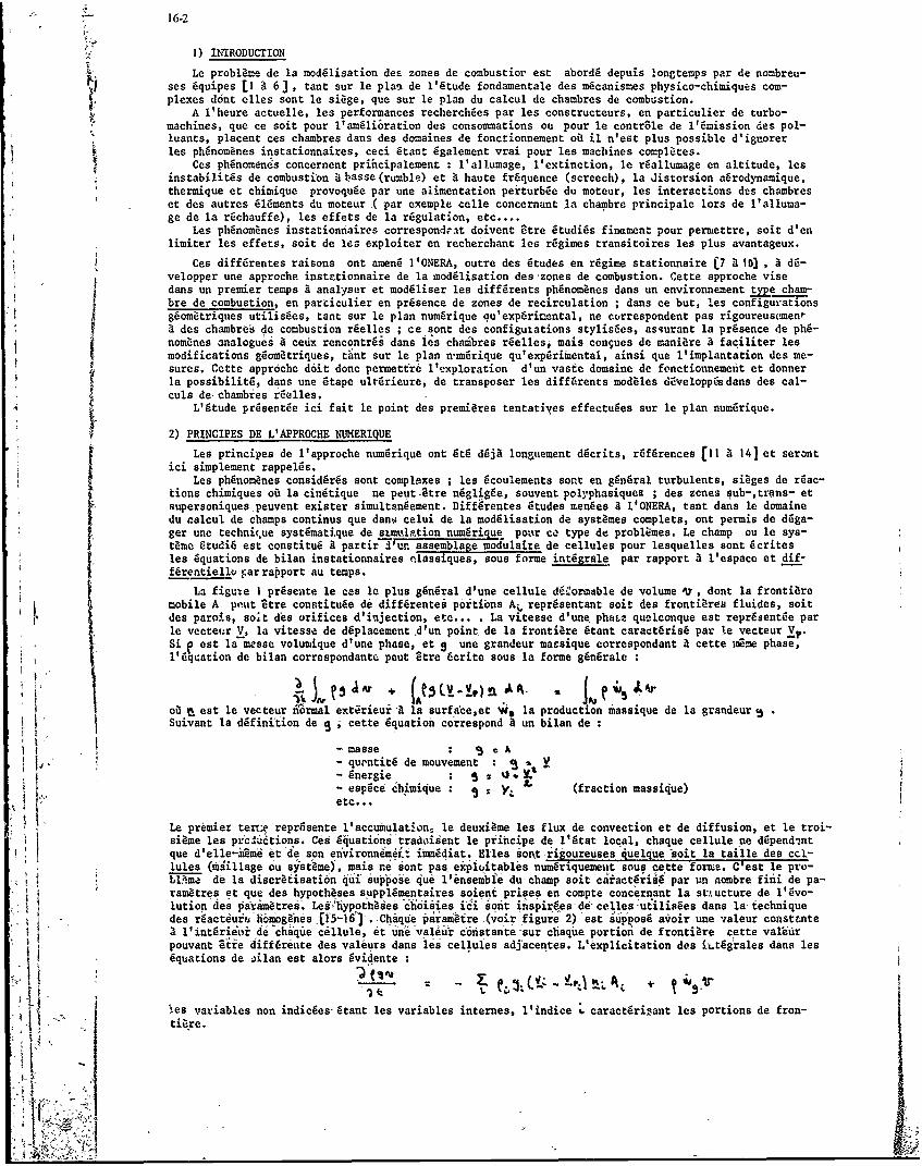
16-2

1) INTRODUCTION

ii Le probl~me de la mod~lisation des zones de combustior est abordg depuis longtemps par de nombreu-ses 6quipes LI a 63J, tant sur le plaai de l'6tude fondamentale des m6canismes physico-chimiques comn-plexes dont elles sont le siage, que sur le plan du calcul de chambres de combustion.

A l'heure actuelle, les performances recherchges par les constructeura, en particulier de turbo-machines, que ce soit pour l'am~lioration des consommations ou pour le contr~le de l'6mission des pol-luants, placent ces chambres dans des dornaines de fonctionnement oi il n'est plus possible d'ign-orerles ph~norn~nes instationnaires, ceci dtant 6galement vrai pour lea machines complates.

Ces ph~nomdnes concernent prificipalement :l'allumage, l'extinction, le r~allumage en altitude, lesinstabilit~s de combustion a basse (rumble) et a haute fr6quence (screech), la Jistorsion a~rodynamique,thermique et chimique provoquge par une alimentation peiturb~e du moteur, les interactions des chambreset des autres 616ments du moteur,( par exemple celle concernant l~a chambre principale lors de l'alluma-ge de la r~chauffe), les effets de la regulation, etc....

Les ph~nomanes instationnaires correspondrat doivent 9tre 6tudigs finament pour pernettre, soit d'enlimiter les effets, soit de lea exploiter en recherchant lea r~gimea transitoires lea plus avantageux.

Ces diff~rentes raisons ont amenE I'ONERA, outre des fitudes en regime atationnaire C7 it101 , A d6-velopper une approche instetionnaire de la aiod~lisation des zones de combustion. Cette approche visedens un premier temps A analyse~r et modgliser les diff~rents ph~nom~nes dans un environnement M .chain-bre de combustion, en particulier en pr~aence de zones de recirculation ; dans ce but, les configurationsgfiom~triques utilisfies, tant sur le plan num6rique gulexp6rirnental, ne correspondent pas rigoureus~menta des chainbres de combustion r~elles ; ce sont des configutations stylis~es, assurant la pr6sence de ph6-nom~nes analogues A ceux rencontr~i dans i~a chamibres r~ellesi mais conqdes de maniare a faciliter leamodifications g~omatriques, tint aur le plan n-m~rique qu' expdrimental, ainsi que ltimplantation des me-sures. Cette approche doit donc permetfr6 l'exploration d'un vaste domaine de fonctionnemeent et donnerla possibilit6, dans une 6tape ult~rieure, de transposer lea difffirents modales d~velopp~sdans des cal-culs de-chambies r~elles.

L'6tude prdsentge ici fait le point des premi~res tentatives effectufies sur le plan num~rique.

2) PRINCIPES DE L'APPROCHE NUMERIQUE

Les principea de l'approche num~rique ont fit ddjA lonpxiement d~crits, r~f~rences [1i A 141 et srn

Les ph~nomanes considgrfis sont complexes lea 6coulements sort en gfinfral turbulenta, siages de rdac-tions chimiques ofi la cin~tique ne peut~tre n6gligde, souvent polyphasiques ; des zones sub-,trons- etsupersoniques-peuvent exister simultantement. Diff~rentes fitudes umen~es A 1'ONERA, tant dans le domainedu calcul de champs continua que danv celui de la mod6lisation de sysames completa, ont permia de d~ga-ger une technicue aystgmatique de silto u~iu pon1 ca type de probl~mes. Le champ ou le sys-tamo 6tudi6 eat constitufi A parti r iassemblage modulaite de cellules pour lesquelles sont 6criteslea Equations de, bilan instationnaires '.lssiques, sous formne int~grale par rapport a l'espace et dif-fdrentiellv rarraoport au temps.

La figuie I pr~sente le cas le plus gfingral d'une cellule d6k'orinable de volume 'V , dont la frontiaremobile A pfnut Btre contitituge d& diff~rentei portions A, repr~sentant soit des fronti~res fluides, soitdes parois, so~t des orifices d'injection, etc... . La vitesse d'une phaoe quelconque eat reprgaent~e parle vecteur V. la vitesac de d~placement ~d'un point de la frontiare 9 tant caract~krisd par le vecteur V,Si Yeat la mzsae volumique d'une phase, et Sune grandeur ma*:sique correspondant A cette varne phase,l'6quation de bilan correspondanto peut 2tre Ecrite sous la formne g~n~rale

r A , % 14eioa eat le vecteur Ciorinal ext;_rieui-a la surface,et *4Ev la production massique de la grandeurf3

Suivant la definiteion de Sicette Equation correspond A un bilan de

- masse A- qurntit6 de mouvement 43 Y- Snergie %3"e- esp~ce chiiique yt (fraction massijue)etc...

Le premier terr reprfisente l'accumulation, le deuxigme lea flux de convection et de diffusion, et le troi-siflme lea pftcliutions. CUs Squati6n8'tradoiient le prihcipe de 1'6tat local, chaque cellule ne ddpendintqua d'elle-remd bt 'de son ativironne"ait iaangdiat. Ellas iox~t-rigourauses quelque -soit la taille des cc4-lules (6gillage 6u syat' me), mais re 'sont pas, expioitables num~riquemeut sous cette forme. Veast le pro-blTma db ia discratisation qui suppose 4u6 l'ensarmbe du-champ soit ciract~rise6 par un nombre finii de pa-ramiztres et que des hypothases suppidmentairas soiant prises an compta concernant la st).ucture de 1'Evo-lution'des paramatrei. Les-l'iypoth~ie6 choiiies ici B oa't inspirges- decelles'uillisdes dana la- techniquedes reiadtiuib aoganea CIi16 . Chque paranittra _(voir figure 2) 'eat spos6 avoir une valaur conatm~tea l'interieut de chaque callula, dt une vlur conistan'te-aur cfiaque portion de frontiare cette valaurpouvant Bii diff6rente des valeura dana lesi cellules adjacentes. L'explicitation des iLt~grales dans leaEquations de Ailan eat alors 6videnta

dlles variables non indicges- 6tant lea variables intarnes, l'indice L caract6ri.;ant lea portions de from-

r

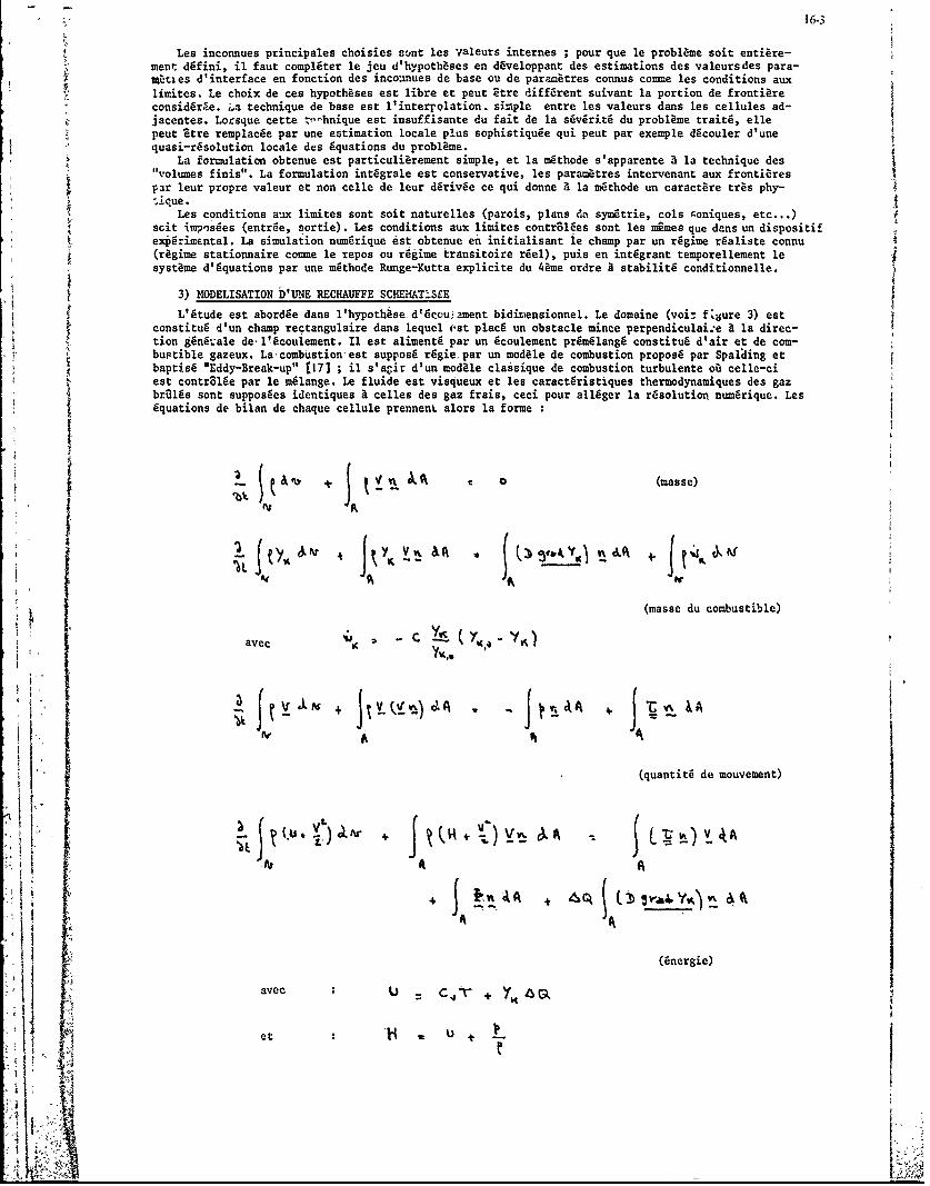
16-3

Les inconnues principales choisies stmnt les Valeurs internes ; pour que le problame soit entiire-ment ddfini, il faut compldter le jeu d'hypothases en dfiveloppant des estimations des valeursdes pars-ecties d'interface en fonction des incounues de base Ou de parainatres cons come les conditions auxlimites. Le choix de ces hypothases est libre et peut Etre diffdrent suivant la portion de frontiarecoosidftre. i.a technique de base est l'interrolation. simple entre les valeurs dans les cellules ad-jacentes. Lorsque cette t,"-hnique est insuffisante du fait de la sfivfritg du problame trait6, ellepeut Ztre remplacde par une estimation locale plus sopbistiqu~e qui peut par exemple dicouler d'unequasi-rdsolution locale des 6quations du problame.

La formulation obtenue est particuliarement simple, et la mithode s'apparente a la technique des"'volumes finis". La formulation intdgrale est conservative, les parametres intervenant aux frontiaresp~r leur propre valeur et non celle de leur d~riv~e ce qui donne a la mdthode un caractare tras phy-;±que.

Les conditions aux linites sont soit naturelles (parois, plans dn syaktrie, cols Aoniques, etc...)scit im~esdes (entrde, sortie) . Les conditions aux limites contr~ldes sont les mimes que dens un dispositifexpdrimental. La simulation numfirique est obtenue en initialisant ie champ par un regime rdaliste connu(ragime stationnaire come le repos ou rdgiine transitoire rgel), puis en intdgrant temporellenent lesystame d'6quations par une mfithode Runge-Kutta explicite du 4ame ordre A stabilit6 conditionnelle.

3) HODELISATION b'UNE RECHAUFFE SCHENAMVISEL'Stude est abordge dans l'hypotheised'dccui2ment bidirmensionnel. Le domaine (voir f*,ure 3) est

coostitufi d'un champ rectangulaire dans lequel ('St placC un obstacle mince perpendiculai~e A la direc-tion ggndg.ale de-l'dcoulement. Il est alimentg par un 6coulement prdmfilang6 constitufi d'air et de comn-bustible gazeux. Lacombustion-est supposfi rdgie par un modile de combustion proposg par Spalding etbaptisd 'Eddy-Break-up" E171 ; ii slacir d'un modale classique de combustion turbulente oa celle-ciest controlfie par le mdlange. Le fluide est visqueux et la caractdristiques thermodynamiques des gazbralgs sont supposges identiques a celles des gaz frais, ceci pour alldger la r~solution numfirique. Lesdquations de bilan de chaque cellule prennen. alors lafom

~ j' .n (masse)

(masse du combustible)

avec -C Y4, -K+ aVv)oi A jCr% &

(quantitfi de mouvement)

'j 41A 4 j A

(6nergie)

avec C 4r YAcis

et 0

16~4

Y.est la fraction matsique de combustible, Y%.. celle correspondant au prdmalange,'b le coeffi-cient de diffusion, iwK la production de combustible par unitl de masse, C une constante du modalede combustion, T le ren-3eur des forces de viscosit6 qui depend du modie choisi, U l'6nergie in-terne phys5.co-cgimique, H l'enthalpie physico-chimique, Ile flux thermique et Aq la chaleur decombustion. Les rdactions chimiques sont schdm~tisles de Eagon simple par une -.eaction globale uni-que entre le combustible K et le comburant 0 , donnant des produits de combustion entiarement bril-16s

X Vo 0 - '

Le domaine est dilcomposi en collules rectangulaires identiques. Le passage aux 6quations discri-tis~es exploitables num~riquement, effectul conformilment a la technique d~crite au §2. , est ilvidoeltet ne sera pas d~taillg ici. Les traitemonts d'interface choisis different suivant qu'il s'agissed'interfaces ordinaires ou limites. Au niveau d'interfaces ordinaires, les valeursdes parami~tres sontles moyennos arithmiltiques des valeurs correspondantes dans los cellules adjacentes. Au niveau des pa-rois, la vitesso eat nulle, los d~rivges spatiales des composantesde la vitesse, intorvonant dans lestermes d'effort sur les frontiares dens les 6quations de quantit6 de mouvemont , sont modillis~es demaniilre a restituer le frottement local, les prensions et tempilratures sont 6gales i leurvaleur dans lacellule (gradients locaux nuls ). Aux interfaces d'entrde, la pression d'arr~it, la temperature d'arr~tet la composition sont impoages fonction du temps, la vitesse iltant d~duite par extropolation des vi-teases A l'int~rieur du domaine. Aux interfaces do sortie, seutle la pression statique es,impoade,tous lei autris parain~tres 6tant extrapol~s.

La simulation num~rique est rdalisge en deux 6tapes :mise en mouvement A partir du repos, do l'6-coulement sans combustion, jusqu'A obtention d'un ragime stabilisl, puis initiation de la combustionen aval de l'obstacle.

La mise en mouvement du fluido est obtonue en augmentant progressivement (Sins) la prossion d'arrat(de 50.000 a 52.000 pascals) et la temp6rature d'arr~t A' lentrde, simulant la compression isentropi-que d'un rilservoir 5iLUl A I'amont, et en maintenant constante la preasion do sortie (50.000 pascals).La figure 4 prdsente des cartographies de vitesse aux temps t = 3 - 8 et 13 ma, montrant un 6coule-ment tout d'abord coll6 aux perois, puis le dficlenchement progrossif de la zone do recirculation A laPointe de. l'obstacle et son dfiveloppement. La figure 5 prilsente la configuration d'6coulement obtenueen rdgime asymptotique mettant en 6vidence une zone de recirculation longue (8 fois la hauteur do l'ob-stacle). Co r6sultat correspond A un modale de viscosit6 turbulente homogane importante , tTO'ALa figure 6 pr~sente Ofivolution temporelle do la 'iitesso d'entrfie et de la vitosse de sortie au mi-lieu de la portion libre du ctnal.Los iscillations mettent en fividence Los temps caract~ristiques(10 ma) de propagation des ond's dans le canal ; le temps global de miso en viteaso ( '!e 4o rftcaract~rise l'inertie de la coltonne gaz~use ; le d~calage progroasif doadeux vitesses caractdrise ledfiveloppement de la 2one de roci'zculation et des portes dues aux effets visqueux.

L'initiation de la combustion eat obtenue en supposant quo le combustible contonu dana la collulesitu~e au centre de la recirculaticn br~le instao~tan~ment . La constante C du modale do combustion eatprise ici 6gale 500 . La figure 7 prisente des cartographies do tompdratures obtenues A des instantssucc(-ssifs en maintenant conatantes Lea conditions aux limitos. Ati debut do la sdquence, Los processusde diffusion thermique prennent le pas aur la combustion et la zone d'initiation se ref roidit au pro-I f it des cellules environnantos. Par la suite, la combustion doveaant plus intease, le niveau gn~ralde temp6rature augmento. Le procossus 6tan'. trUc rapide, la masse contenue dan. lea cellulos oO so pro-duit la combustion vanie peu, et la pression eugmente consid~rablement devenant largement sup~rieureIaux pressions impoades aux deux extr~mitfis du champ ce qiti provoyie un refoulenont a l'entrde e. A lasortie, ph~nomane rdaliket, mais me permettant pas d'attoiudre un r~gime stabilisl.

Pour %:viter ce phgnomane, ti pilotagedes conditions aux limitea d'ontr~o a W mis au point rdali-sent la simulaton d'une alimontation par col sonique d~samorgd , l'onde de choc so plagant a proxi-mitfi de la secl.ion d'entrde ac r~agissant instantan~ment A 1'fivolution des conditions dens cette sec-tion. Ce sont t-,u~oura lea pression et tempfirature d'arr~t amont qui sont imposges: la pression d'ar-r~t, au lieu d18tre maintenue constante eat continuellemer'. r~ajustae de maniare A induiro un debitO.'entrde constant, la tempdrature d'arrat eat maintenue coitutante.

La figure 8 prdsente lea r~sultats obtonus dams ces conditions. Pendant Lea premiers instants, leprocesaus eat identique a coldi du cas prdcddent mais d~s que la preasion dana la zone de combustionaugmente notablementi lapression d'entrge'rdagit et augmonte 6ntrainant une convection de la zone decombustion vera Ilaval. La fraction de gaz chauds restant derriare l'obstacle provoque L'inflammationdes gaz frais d~passant L'obstacle et une douxiame poche de combustion oat form~e. Le processus sepoursuit jusqu'l obtention vera t - 75 ma d'un rdgime enti~rement stabilists oa la zone de combustionse d~veloppe lat~ralement a1 parti~r de la zone do recirculation avec laquelle ello se trouve en 6quili-bre dynamique it gnorgdtique. La zone de' redirculation eat alors considgrablement plus courte.

:A figure 9 prdsente l'volution temporelle de la pression statique dana la cellule oO lLa combus-tion a dtg provoqu~e et de la pression d'arr~t a l'entido. Los oscillations sont le r~sultat du couple-ge eDZre lea conditions d'entrfie et la combustion. Le ddphasago peu important entre lea deux profilseat dii a la faible distance entro L'entrge du domaine et le point d'initiation.

Los r~sultats suivants concevtnent la compereison entro Lea iggimes stabilisgs sans ot avec com-bustion. La figure 10 prilsente Les profils longitudinaux de vitesse pour deux lignes situ6es dana lapartie libre et dana la partie obstru&e du canal. Ello met on 6vidence I'ecc~l~ration de L'gcoulementdie a la combustion. La figure 11 pr~seute sur ces memes lignes l'ea profils do tempilrature. La figure12 reproduit des profils tranaverseux lo temp6rature et de vitesse, l~garement en av,,I de l'obstacle,dana la zone de recirculation. La figure 13 presente des profils longitudinaux do pression statiquedams la partie libre du canal ; lour forme oat classique do ce typo d'6coulements. La figure 14 pr6-sente pour diff~rentes positions transversales, des profils longitudiiaix, do fraction masaique do com-j bustibla mettant en 6vidence le dogr6 d'avencornont 1e plus Elev6 do la combustion dens la zone de re-circulation bien quo limit ' par le nivoau des Achanges do cotto zone avoc le fluide saiii. La veliditldos r~sultats cbtenus du point do vue do la combustion no sera peas discut~e ici car ello oat essontiel-lement lige aux mod~leob choi'nis.

16-3

La modilisation des effers visqueux: reste un problame d~licat. Des modales de turb"lencc ant Wessay~s qui permettent de retrouver des r~sultats voisins di ceux obtenus ici, cependan- ce,. r~sultatssont extr~mement sensibles aux valeurs desconstantes introduites dans les modalzs. Cependant, cette Etudemet en Evidence la capacitg de la m~thode a'aborder 1'6tude des regimes transitoires lors de 1'allu-mage d'une r~chauffe oil le dfibit d'entrge eat 6galeument fixg, et la possibilitl d'acc~der aux: niveaux

de perturbation, Problme important pour les motoristes.

4) APPROCHE DE LA MODELISATION D'UNE Z ONE PRIMAIRE SCHEMATISEE

Une Eltude de modilisation de zone primaire a 6t engagde, en collaboration sur le plan exporimen-tal avec l'ilquipe MAGRE-HEBRARD (183 , dans l'optique developpe au §1. La chambre de combustion rfia-lisfie pour l'iltude expirimentale (voir figure 15) est composfie de deux voltdmes parall~l~pipddiques misen communication l'un avec l'autre par des orifices decaractlristiques ajustables tenant lieu d'orifi-ces pfimaires. Le fluide traverse complatement le boltier d'alimentation (volume infdrieur), une partiedu flux pdn~trant dans la chambre (volumesupdrieur). Les deux dilbits sont rilglils par des cols soniquesplacds dans le m~me plan A la sortie de la maquette. L'irjection du car!burant peut Ztre rdalis~e pardiffilrents syst~mes :cannes de prfi~aporisation, inje--teurs tourbillonnaires, etc... . Un programme decalcul tridimensionnel a Wt r~alis6 sur le meme principe que le programme bidimensionnel d~jA prdsent6.Le domaine de calcul (voir figure 15) correspond strictement a la giomitrie d'une cellule 616mentairede la chambre expilrimentale. Tes r~sultats prdsentls ici correspondent, aux premi-1res tentatives de cal-cul sans combustion.

La technique de simulation de la prilsence des cols des deux chambres ayant prilsentd des difficultdsde mise au point, la technique de contr~le des conditions aux limites utilisdes en bidimensionnel aWreprise ici. La pression d'arr~t a l'entr~e du boltier d'alimentation A 6t6 mortfie en 5 ms de I0O.COO A108,000 pascals, la pression siatique de sortie du mieme bottier a Wlt montile dans le meme temps de100.000 A 105.000 pascals, la nression statique de sortie de la chambre a 6t6 maintenue constante. Lafigure 16 prilsente les fivolutions temporelles des debits d'entr~e dana le boltier d'alimentation (E),de sortie de ce boltier (A), dans l'orifice primaire (T) et de sortie de la chambre (C). Elle met en fivi-dence les ddphasages entre lea difffirents points du domaine et le temps caraci~ristique inertiel (-2 or.S)Le dilbit priuaaire en r~giine stabiiisl correspond a 15 % du d~bit totat.

La figure 18 prfisente des cartographiesde vitesse (6chelle logaritiazaique) pour le regime stabilisl.La configuration de 1'cueet complexe, fait apparaltre des zones de recircu.lation en fond de chain-bre et lat~rales par rapport au jet. La valeur relativement peu 6levge du d~bit primaire et Ia forteviscosit6 (J&ve,A) expliquent l'inclinaison modgr~e du jet et la faiblesse de l'impact Sur Ia paroi oppo-see. L'llr du profil de vitesse en sortie de chainbre eat dO aux diff~rences de pertes de pressiond'arr~t entre les diffdrents filets de courant. Les r~sultati expdriinontaux correspondant ne sont pasencore disponibles. Des calculs sont en cours pour des niveaux de viscosit6 plus faible et un domaineallong6. LA encore, le modale de viacosi;., a une grande influence sur les r~sultats.

~)CONCLUSIONLe rrincipe de l'approche adoptie par 1 .)NERA, potr lea iltudes eu r~gine instationnaire des zones

j de combustion avet. recirculation, fondd sur une simulation num~rique dans des configurations de chain-bre sch~iatiedes, permec d'aborder l'4tude des rdgimes transitoires qui in76ressent actuell-ment lea mo-torisces. Elle oe situe A la-jonction de l'analyse des mdcanismes foidamentaux de la combustion turbu-lance et de Ia prdvision de laura offets dana 7.1environnement d'une chambre de combustion. Lea r~sultatsobtonus acuelleinent $onc partiels mais ratrowent ddja l'importanca des fluctuations do pression borades phases d'allumage ; le programme de calcul tridiinensionnel, qui, avec un nombra de maillas raisona-ble (2400 cellules de I cm de c~tfi), aboutit A des descriptions d'~couleinents dojA complexes, sera uninstrument officace, at la confrontation des rdsultats obtenus avec lea r~sultats expdrimentaux corras-pondant, tant en regime transitoiii qu'an r~gima stationnaire, doit permettre V' elaboration et Ia va-lidation de modales de curbuleiice et dc combustion r6alistas et cransposables 5 des chambros induscriel-lea.

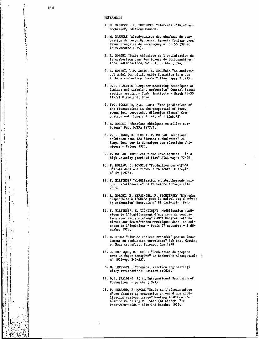
16-6

REFERENCES

1. M. BARRERE -R. PRUDHOMME "El-ments d'Alrother-mochimie', Editions Masson.

2. M. BARRERE "Afrodynamique des chambles de com-bustion de turborgacteurs. Aspects fondamentaux"Revue Fran~aise de Mcanique, n' 55-56 (3a et4E ti±mestre 1975).

3. R. BORGHI "Etude th~orique de l'optimisation dela combustion dans les foyers de turbomachines."Acta Astronautica, vol. 1, p. 667 (1974).

4. R. ROBERT, L.D. ACETO, R. KOLLRACK "An analyti-cal medol for nitric oxide formation in a gasturbine combustion chamber" AIAA paper 71.715.

5. D.B. SPALDING "Computer modelling techniques oflaminar and turbulent combustion" Central Statessection meeting - Comb. Institute - March 28-30i (1977) Cleveland, Ohio;

6.1F.C. LOCKWOOD, A.S. NAGUIB'"The predictions ofthe fluctuations in the properties of free,round jet, turbulenti dif-iusion flames" Com'-bustion and flami,vol. 24, n* I (feb.75)

7. R. BORGHI "Rgactions chimiques en milieu tur-bulent" Pub. ONERA 1977/4.

8. V.P. SINGH, R. BORGHI, P. MOREAU "Rdactionschimiques dans les flaimnes turbulentes" 2e.Symp. Int. sur la dynamique des rfactions chi-miquet - Padoue 1975.

9. P. MOxEAU "Turbulent flame developement in ahigh velociy premixed flow" AIAA naper 77-49.

10. P. MOREAU, C. BONNIOT "Production des oxyde&d'atote dans Une flammeturbulente" Entropien' 69 (1976),

II. F. HIRSINGER "Moddlisation en adroehermodynami-qeinstationnaire" La Recherche Afirospatiale

i i 79-5.

12. R. BORGHI, F. HIRSINGER, H. TICHTINSKY "fthodesdisponibles a I'ONERA pour le calcul des chambres

' I de combustion" Entropie n* 81 (mai-juin 1978)

13. F. HIRSINGER, H. TiCHTINSKY "Moddlisation numd-rique de l'tablissement d'une zone de coiabus-tion avec recirculation" GAMNI Congras interna-tional sur lea m6thodes numnriques dams lea sci-1I ences de l'ingfnieur - Paris 27 novembre - I d6-

• I cembre 1978.

14. D.DUTOYA "Flux de chaleur transf~rd par un 6cou-lement en combustion turbulente" 6th Int. MeetingJon Heat transfert. Toronto, Aug.1978.

15. J. DUTERQUE, R. BORGHI "Combustion du propanedans un foyer homog~ne" La Recherche Afrospatialen* 1975-6p. 347-357.

16. 0. LEVENSPIEL "Chemical reaction engineering.Wiley International Edition (1962).

17. D.B. SPALDING 13 th International Symposium ofCombuation - p. 649 (1971).

18. P. HEBRARD, P. MAGRE "Etude de l'a~rodynamiqued'une chambre de combustion en vue d'une modd-lisation semi-empirique!' Meeting AGARD on cca-bustion modelling PEP 54th (B) Linder Hohe4 " Porz-WahnrHeide - K"ln 3-5 octobre 979.

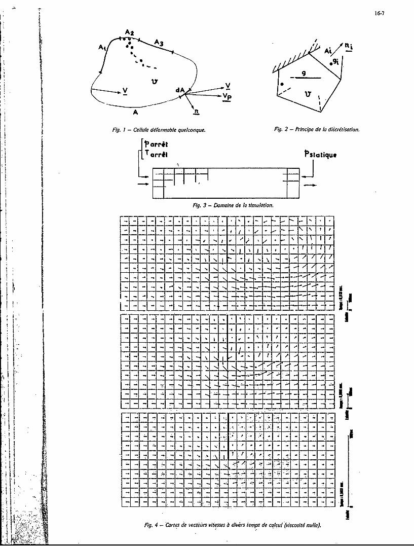
16-7

AA

Fig. 1I Ceivile diformoble quelconque. Fig. 2 - Principe de /a di.icrtisation.

ia rriI

T arri IPstatique

Fig. 3 - Domaine de la simulation.

**-TT-*-- -.777T-

I- ~ W! Nd ~ ' .~ T 7

K --- : -4 Z4....2-L4 -7.

- 7I

4 4 -4

01"1

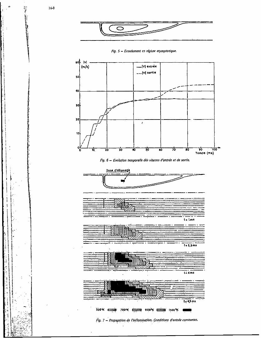
16-8

Fig. 5 - Ecoulement vn rigine asymptotique.

60 -v - -

(mis) ~-lVl entre

So- --- IvI sortie

20

V0 10, 20 30 40 So 60 70 so 90 10Tamps (ins)

FRg. 6 - Evo luion tempo relle des vitesses d'entrie et de sortie.

Zone d'allumo

t, S.ms

I urn r//77n7

300K ?007OK, E??? UO00K' MMM Iso0K E i

f~g. 7 - Propagation de lI~fiflam~natl6n. -Conditions dlentrde constantes.

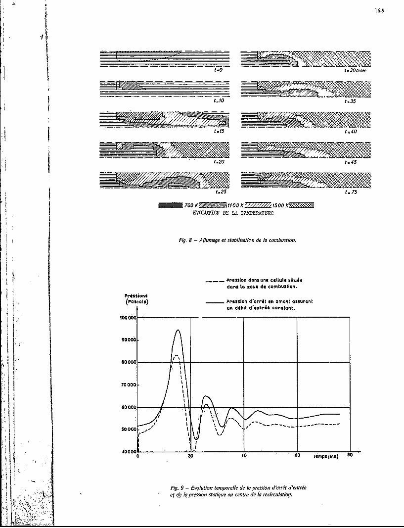
16-9

It=10 t.35

It.15 t.40

1t.20 t%45

I t..25 t.*75

700K=VIOK 500 KEVOLUTION DE LL. MERNTUIfl'

Fig. 8 - Allumoge et stabillsotlen de la combustion.

Piression dons une callult vitit

Prosionsdons to motto do combustion.

(Pascal$) Prsion d'arrit on amont assurontV un dibit d'entrie constant.

IL 90000

SOOOC.

0 0 40 60 TirpS (ms) 80

Fig. 9 - Evolution temporelle de Ia oression d'arrit d'entreeet de Iq pression statique au centre de to r-ecirculation.

-4

16-10

Niveau d ovec combustion

-- dfaphragme --- sons combustion

Ixz ---------------- -----------

,0,2 0 02 04 06 A , , ,02ovec'combustion sons combustion

II Point de recollement t

Fig. 10 - Pro fls longitudinaux de vitesse - Combustionstabiiisde (t =75 ins).

diaphrcigme

Pon do

- 0,I 0 ',2sIziG-m

WOO ),____ Fig. 'I - Profilslongitudinaux de remptirature - Combustion

K t~ s/s)stabllie (t 7j~ ms)I.

1500 g.1SPo fl/s transversaux de.temratr t tse

- iso ~ Cmbustion stabisde'(t =75 mns).

lid-~

ISc~ - - avec comnbustion

_____ ..... .. sns mbustion0, 0.4 (m)i 0P .m -

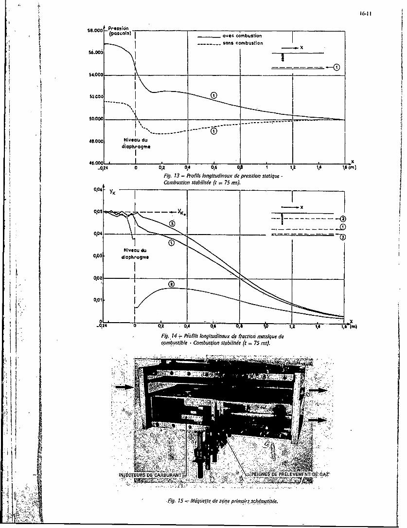
16-11

S85.000 ,sinasot avec combustion

------ sons combustionj 56.000

52.000

50.000

1----------

48.000 Nlveau du

diaphragme

-0~..24 0 0,2 0,4 046 Oe114 -, m

Fig. 13 - Pro fils longitudinaux do presstlon statique -

0~0~ YI(Combustion stabllisde (t =75 ins).

0,05 .

0,03. diaphragm*

0.0i

K FR4.'14 - Pib f/s long/wudlnaux de fractioni imssique decombust'ible -Combuitlon stabillsie (t= 75 in).

1 4

I C 4vIsI

INJECTEURS' C~ABRN ~ ~ p PtNSERLE EMFNTs0EGA

< i~g. 15 -Maquete de zone pnmair'scditsee

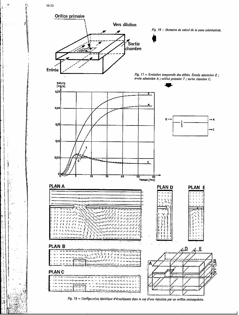
16-12

Orifice -primaire

,~i. Vers dilutionFig. 16 - Domaine de ca/cu/ de Id zone schcmatsde.

Enre

chmr

Entr~eeFg. 17 - Evolution temporeile des ddbits. Enree admission E;smrtie admission A ;orifice prima/re T; sortie chombre C

Dibits(k /S)

0,25

-I 0,20

I I-

0,05

Temps (ms)

PLANA PLAN D PLAN E

IZ; -------- ;I ~

I I-.----- II___/_%_II ,

f -/111/

4, 1'

PLANGB

'Fig. -18 - Cbig~t,-Vr thdorlque'dcouldre)t dons le cas d'une injection par ur, orifice rectagulaire.

1.7-I

ANALYSIS OF LOW-FREQUENCY DISTURBANCESIN AFTERBURNERS

FRANK E. MARBLE, PROFESSOR OF ENGINEERINGCalifornia Institute of Technology

z05-45Pasadena, CA, 911t5

MALLADI . SUBBAIAH'SEBASTIEN M- CANDEL

'SUMMARY

The transient response of large burners depends primarily upon fluid mechanical adjustment ratherthan upon a time delay associated with chemical- response. Examples of this behavior are the non-steady behavior of burners' in utility. boilers,- and-the low-frequency response of afterburners in air-craft gas turbines. Previous investigations have shown, that the distorted flame interface duringnon-steady operation causes an activ e response to acoustic input at selected frequencies. This re-sult depends upon fluid dynamic behavior of the gas of very differeut densities upstream and down-stream of the flame front.

In the present work, the behavior of these 'stabilized flame zones are-examined when they aresituated 'in an'afterburner. The turbine dischargeand the nozzle inlet planes are represented byappropriate admittance functions for low frequencies. The distances which separate turbine dis-charge, flame holders, and nozzle throat, as well as the number of flame holders, are parametersin the problem.

The results show that small disturbances which originate in combustion roughness, may be amplifiedto serious amplitudes and the amplitude level is a strong function of the geometric parameters ofthe flame-afterburner arrangement. In some instances instability may resdlt.

I. INTRODUCTION

Combustion noise and combustion instability in 'propulsion systems frequently is associated with theresponse of the combustion prucess to local pressure and velocity disturbances and to the acousticcharacteristics of the complete system (1, Z). The frequency spectrum that is important dependsupon the acoustic'modes of'the system; in gas, turbines and rocket motors, the frequencies oftenlie in the range of seerai hundred--to several th'ousand ,cycles per -econd. When tho frequenciesare of the order of a kilohertz, the ratos of the chemical reactions contribute to the time delay inan essential way (3). Using this fact it has been possible to scale the results of experiments oncumbustion systems utilizing various fuel 'types (4) and different g'eometric configurations. Forfrequencies of, say, 100 Hertz or less, the chemical times are less important and other featuresof'the combustion system 'determinethe detailed response of 'thle burner. Recently two of 'us (5)considered a flame stabilized at the center of a two-dimensional channel of infinite length, by acentral body of finite size. Under steady operation the flame spreads, from the center body to theduct wals; when the combustion Process between the burned and unburned gas can be characterized,the flame shape and the flow field may be calculated. This steady configuration was then per-turtied by in 'acoustic wave, the bodies of' high;-density ,gasi pi, 'and low-density gas, p, weredisturbed 'nd' the 'flame' inteiface,,distorted to' accohmodate these disturbances, The process ofrecovery to the steady-state flame shape constitutes the "response" of the combustion process;

' the magnitude of the response and its time delay are thus features of the combined transientmotion of the gas and the flame front;, The, results of calculations based on this model showedacoustic -transmission and reflection coefficients indicating signal amplification at certain char-acteristic frequencies. It appeared, therefore, that with certain reflection conditions ahead of

band ehihd the' burner, 'large pressure' oscillation levels could',be maintained' and, perhaps' in-stability. -

The present investigation applies the results of our previous investigation to a rudimentaryafterburner" configuracion. The work constitutes the first step in constructing a rational modelfor low-frequency disturbances in afterburn~rs.

' Z.: 'ANAL YTICAL DESCIPTIION: OF A'N6N-STEADY- STABitIZED' FLAME

Consider a flame in a duct of half-width 4 , fixed at a point near the centerline by a flame holder,Fig. 1. The flame is described as a sheet, thin in comparison with other significant lengths ofthe problem, and characterized by a local flame seed w, which denotes the component of gasvelocity, 'normal to, the flame on the upstream side, measured relative to the flame sheet. Theposition of the flame 'sheet is described by its distance (, ,) from the center line of the duct,the x-axis. Neglecting gravitational effects, the flow fields ahead of the 'fladme, region 1, anddownstream of the flame, region 2, are described by equations' of continuity and motion

A + (1)

Pt ,'::: ( 2)

17-2

(3)

'together with the thermodyfiaiiid relationVt Vt v. Pt(4)

which states that there are no entropy-producing mechanisms apart from the flame itself. Thevariables describing the upstream and downtream fields are indicated by subscripts 1 and 2. Thestate of the gas far ahead of the flame is uniform, irrotational and of uniform entropy.

Figure 1. Notationand- Geometry, for Flame, Stabilized in Duct.

The two flow fields are matched across the flame sheet by mass and momentum conservation rela-tions and by ,the, kinematic conditions,that the flame sheet. and the flow ,fields deform in a consistentmanner. These kInematic- conditions resemble, that at. the liquid surface in' conventional wave theorybut here there ar,,fixed propagation speeds of the surface with respect to the upstream and down-stream fields. These relations are

(0, t) 22 (, 4 W. 6 5eC U(5)J

.14j 4 W, See 0jfA ax (6)

where %9- is the local angle between the flame sheet and the x-direction, wx is the normal flamevelocity, defined on the upstream side of the flame, and wg is the corresponding quantity downstreamof, the flame.

Conservation laws across the flame- sheet-are applied in reference frame, of the flame itself and in-volve values of .the field variables at the flame., )Mass conservation takes the form

I', , t" f w (7)

r' which defines the value of wg. in equation 6. The momentum balance normal to the flame surface is

l+(8)

and because~the pressure is. continuous alongthe -flame, the nomentum component, parallel to theflame surface is conserved :and reduces tothe condition that the tangential velocity component isconserved.

The combustion process, within ,the flame produces an increase AH in stagnation enthalpy which,because it is large in comparison with the change in kinetic energy, permits writing

(i'a'/p.('ts/~~Y N ~(10)

Moreover, according to equation 8, the pressure ratio across the flame is of order of theqsqu are of the Mach number based> up~n--the, flame 'proagaition speed. It is quite satisfactory

to neglect this ,pessure chaiige asit affect "the temperatue, ratio across the flame, but it isessential in the momentum balance and in determining the shape of the flame sheet. Then withvery, good accuracy

and hence from equation 7,

4'~ (1,

17-3

3. THE INTEGRAL RELATIONS

The description of'a stabilized flame that is disturbed by plane acoustic waves consists of threezones: (1) that far ahead of the flame, in which an acoustic signal originates, (2) the region nearthe flame which responds to the pressure field imposed by the wave impinging from upstream, and(3) the region far- downstream into which an acoustic signal is transmitted as a result of the re-action of the flame zone to the imposedl, signal. There will, of course, be an acoustic wave"reflected!' into the regiono from which the signal originated. Treatment of the gas as incompress-ible in the flame zone simply implies that the large density change which takes place across theflame sheet dominates any small density changes that arise from the acoustic disturbance or fromthe relatively small gai-velocities near the flame.'

The flow fields near the flame zone are described by an integral technique in which the equationsof continuity and motion are integrated with respect to y between the flame and the duct wall. Onthe upstream side of the flame the region of' integration is from X = tz, j) to y = 4 and thecontinui y equation in region I becomes

" + W ( 1 3 )

where we define X,,*, '.Idyas the mean velocity across the region upstream of the flame sheet.Applying the same technique to the equation of motion in the x-direction leads to

at & ax # 9,1, ?' Ae Se 30(14)

and the second equation of motion, equation 3 assures that the variation of pressure in the y-direc-tion is small so that the mean prcssure F, (V j) is nearly independent of y. The similar set ofequations downstream of the flame sheet are

(15)

(16)

The relevant marching conditions, given by equations 5 - 12, may be combined to eliminate thevertical velocity component that no longer appears in the integrated equations. By subtractingequation 5 from equation 6 and employing the conservation of momentum component parallel to theflame sheet, we find that

Ua, 4(4 ) ex e )*,soa

1(Z'~ j -t X~ (a, Co : 0)£VC (17)

where equation 12 ad' the 'fact that . have been utilized in the reduction. Similarlyequation 8 becomes

and hence the pressure drop across the flame sheet is independent of location. Therefore thepressures i't an" vailue of dife ..... ....... .. .. . .. ...'d ' . ... .ny of x differ oii1y by aonstant value, depending upon whether the point is

ahead of or behind the flame.

No difficulty arises in neglecting the pressure variatons with y in each region so that, approxi-matingp.by f:,}) , equation 18 holds also for the difference '¢esti- (.,)The that occur on the right-hand sides of equations 13 and 17 cannot,however, be ieplaced' by tlid corresp'inding verjage' values ai V 4 ,(, if) 'without violatingthe conservation of momentim in the duct. Rather, the matching c6iditions across the 'flaime, must be utilized to approximate local values for these quantities. Calculati.ons of the detailedflow field ahead of the flame suggest that the horizontal velocity component at the upstream l,'..eof the flame surface is well described by

k* t (19)We utilize this approximation and the matching conditions, equations 5, 6, 9, to determine theremaining three velocity 'components in terms of the' flame shape.

4. STEADY STATE AND PERTURBATION PROBLEMS

Calculations based upon these four equations, 13 -. 16, divide naturally into two parts: 'the steadystate 'solution which gives the shape of the'- flame sheet and-the distributions of velocity upstream'4 and' ,dd nstira , and time aependent perturbatlons frm this 'caused acous'tic 'ditirbahces 'thatimpinge up n',the regioii. T epnen variables my e priately as, foe xd mple, ei' .. ... -a' .... a p.....

pn , (a . es m y be (2o)

17-4

where tf4 ,jj is of smallmagnitude determined by the impressed acoustic disturbance. Thenth'tayfaeseti ecie yte zeroth order set of equations, ref. 5, in which

are prescribed at some point ahead of the flame and the condition

(WI ~'s~rJ 9-1Jf, SP ~(21)

relates the two 'Pressure fields. We assume that a, srnall, flame holder exists on the axis of thechannel, so that, thi flame. sheet begifis' a small' di'stance .,,off the x-axis land the upstream flow isapprdpriately deformed inthe viciniiy of the flariie 1.d Imedael o heflmholder the initial value of the g-s velocity' yanfshe3, u,2 (0) = 0, corresponding to conditions be-hind a bluff-body flame stabilizer. The shape and Velocity distribution for a stea~iy, stabilizedflamie is then, determined by integration of these four ndn-linear' differential equations.

Under steady operating conditions the ratio of normal flame velocity uO is. the do'minant parameterwhich fixes the sha pe of the steady flame 'envel6pe. Althotigh the similarity is not exact, the hori-zontal coordinate (*2f)(W-/U. giVes a representation that is independent of M /4. in the range

of interest. This general representation is shown in Figure 2. The dependence, upon the de~nsity

Lfl

0.0 0. 25 0150 0,75 1.00

Figure 2. Steadyr State Flame Shape.

There is considerable empirical evidence indicating that %i - u6~ for turbulent flame zones andtherefore the shape of the flame envelopce is' rather insensitive to changes in ; he approach velocity.

I'These results may be compa 'ed with those 'obtainid by Taien (6) in' his rnbmdel for the steady ductedI'flame and byFabr3. (7) in his more detailed calculations for the same problem. The stea~dytsolutions ihovrn in Figuare 2 form 'the basis of the hon-Steady perturbation_ analysis.

-' Now for the non-steady solution we retain the firat-order perturbation terms from equations 13 - 16,with the result that we obtain a set oi four' linear first order partial differential equations (5) whosecoefficients are functions of x determined fromn the steady flame calculation. The matching condi-tions across the flamne sheet again supply the additional relations requIfred vo determine the com-

plee ~tof diperienifviilbles. E k" cato 8 shows the perturbation pressure to be, continuousacross the flme,''

sthat, in realiy teere ii only a single pre sure perturb~ation variaole. inadiion, becuseth

flame sheet is held'at the flame holder, .(3

IZ (3and the axial velocity perturbation

£~ tj*J o .. wt .(Z4)

is specified by 'thefam hodr orproid .soltitiodis - '*wich is our interest here,these 'becomre a set of Ainear- 'rdinry~differental .equations with variable, complex coefficients.Pressure zkd velocity disturbaie o utside th flame zone axe described by waves of dimensionlessstr'ngth Pand. P 1i,-ihe ,positive, and 'ngative"'--diiections.

To examnine -the hon-steady b6ivior_ we consider two cases. First, let a periodic pr~essure -waveofst~nthpt ad d fz freqiuecy w'-imnpinge I±roin uitr)fstrngtnPof srelgted fhm the radane zoije ~'da aeo A pressure wave cfsrngh

is rfleced hm,,he fam~ zd~'ih a, ave'f t-i~' " ransmitied to hie- right, 'down-'stream .of- the flame z'on e. Because ther e is no acoustic Ave that radiates into the flame zone

frmdowntreami, P2 . Thi correspondng. acaustit, matching conditions with the ouinto the 'differential equations in the flame z6A6 'deterilnes 'the complete solutions for this particular

-'The piessure transmission and reftection coefficients are of primary imnportance because it is

I__

17-5

these quantities that couple the non-steady, combustion -process with the behaevo fa nieofurnace in which it is situated. For Cr.se 1, in which tile acoustic input P1 approaches from up-stream, the transmission coefficient Is T, P/Pr while the reflection coefficient is R - Pz7/PFboth of which are complex. The magnitudes ITI R)Ift and phase f and #i for thetransmission and reflection coefficients are shown in Figure 3 for an acoustic disturbance aheadof the flame. The Mach number of the approach flow is Mo =0. 2, the flame velocity w1 /uO= 0. 1and the density ratio u4. S . The magnitudes of the transmission and reflection coefficients

I TI c

Figurc. 3a. Acoustic Response; Wave From Upstream. MO 0. Z,

wi/O=0. 1, pi /pa 4. S.

a) Transmission - Coefficient Magnitude, IT TI andPhase, ~

UlU

W1 /uO= 0. 1, pl 1/p= 4.'5.b) Reflection Coefficient Magnitude, I RI and Phase,

1i.show well-defined peaks it certain values of 'the reduced frequency wt, /uo. The maximum valuesof these coeff!1leii are of riiiaikable strengthi and itiie -well to remember that because the

* combustion process is active and may feed acoustic anergy into the system, the classical implica-tions of "reflection" and "transmission" are inappropriate. The corresponding results for different

selection of reduc 4 frequencies.

Second, let apiessiiie wave, of 'str~ength Pi imp nge upon the flame zone from the region down-stream of the--flame . A consideration similar to that -above gives the relationship between thefield variables on the downstream edge.'

Because the--acoustic di turbanoce P~ originates downstream of the flame zone, the transmissioncoeffi~ietit is 'T =P_/P wile the' reflection- coefficient is. R - P1/P. Th mgiue and phasere

of these quantities A6e hown in Fguye 4"for th6 game set of la?he onditions as those for Case It

sobseve as- Fgri3 -Wete A u ,e-iiin ,eid6;ntrarm, a similar get 6f'-Oressure peaksis -. erd- as rhe ,physical initrpretatioh 6f-'this iep~nSe Js-diicussed in reference 5.

Consider a rudientary 4fterbuiher 6-'onfgrto fcnth rs etoi ara;b~e plane of thehodr "s loc6ati, At ' =, 0-nd ther are four fla me holder poirio a oss 'the diameter (two

~rus thdimeerof the burne lie D, te ' alue-of- -in' dri flame calculation ,is D/8.6 th Aubi~ i~hige is o~a -'-_s~ne'l afe'ad~of te~fameh,)derplane, the flame

hisa lenith. "L ' ~dh ' "6zk -throat us lociied'a-d in6 a sra froim the end-'of

e- .s nozz e t ralf Thxis th& _z ~i'a sloae t k L+

r 17-.

CY

0o 2 3 6

Figure 4. Acoustic Response; Wave From Downstream. Mo 0. 2,wl/uo = 1., PI/P2 = 4.5.

a) Transmission - Coefficient Magnitude, I TI andPhase, (.

IR

414

Figure 4. Acoustic Responses; Wave From Downstream. M = 0.2,

w1 /uo = 0.1, pl/pa = 4.5b) Reflection Coefficient Magnitude, I RI and Phase, *.

In !,ie regions outside fLame zone the pressure and velocity fluctuations of a plane waveacoustic field may be written _

a ~ ~ * *~(uc) 't(25)

(26)

where u and c are the local0 gas and sonic velocities respectively; P and P7 are the complexamplitudes of the, for wardand 'backward 'running waves. Then, if we define the admittance functionV(x) to be

then substituting from above, we may represent the, ratio of P" to. P+ at any point x as

ih '( (i -,flP -~~e (28)wheie4 a u/c is the-14 al Mach number.

It is then a pstaightforwa~d problem. in on6-dirnensional ac6ustics to match wave fields in-L 9 'x S 0 itihth6 turbine adirpitance at x' -L aind the'"flaime reflection coefficient 'at x 0.Litewise a wave fild ln the region L Sn a L + 1Ia may 'be 'd'evi'sed that matches with the end ofthe flame z e, x'= L, 'and satsfiesithe nozzl6, dmittance'.at x= L -+ L2 .

With AW -formilation, calculations were made -of the response of the burner to a unit input ofprescribed fiequen~c • located at 'i =--0, the flame holder-plane.. Figure 5 shows pressure responsespectra f6t* aset 'of caliultifis made for Mo 0.2,Lv/ 5.2, LI. '= 10 "hd'L /' ' 26.' Thevalues 6f -the acoustic aaiitt~nc6 at the turbine and the nozzle -0. + 1.) 0. 1

r'these 'ce ning, to a nearly choked nozzle. The 'ressure responses,p i, mado dimensionless. .. by the mpsed pressure amplitude -Op . .are shown in Figures 5a, 5b, 5c,

Sd i mtensio~nd othes e core d i e, nwee L 25

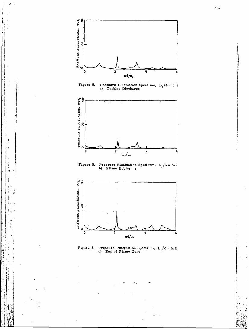
17-7

1'4

0C4

IC,

10 2 46I wi/u.

Figure S. Pressure Fluctuation Spectrum, L AL 5.2?a) Turbine Discharge

0 2 4tU 6

Figure 5. Pressure Fluctuation Spectrum, L /t, 5. 2~~ b) Flame Holder

.- C

2 4

WIO

~1 Figure 5. Pressure Fluctuation Spectrum, L1 AJ 5. 2c) Eiid of Flame Zone

&1

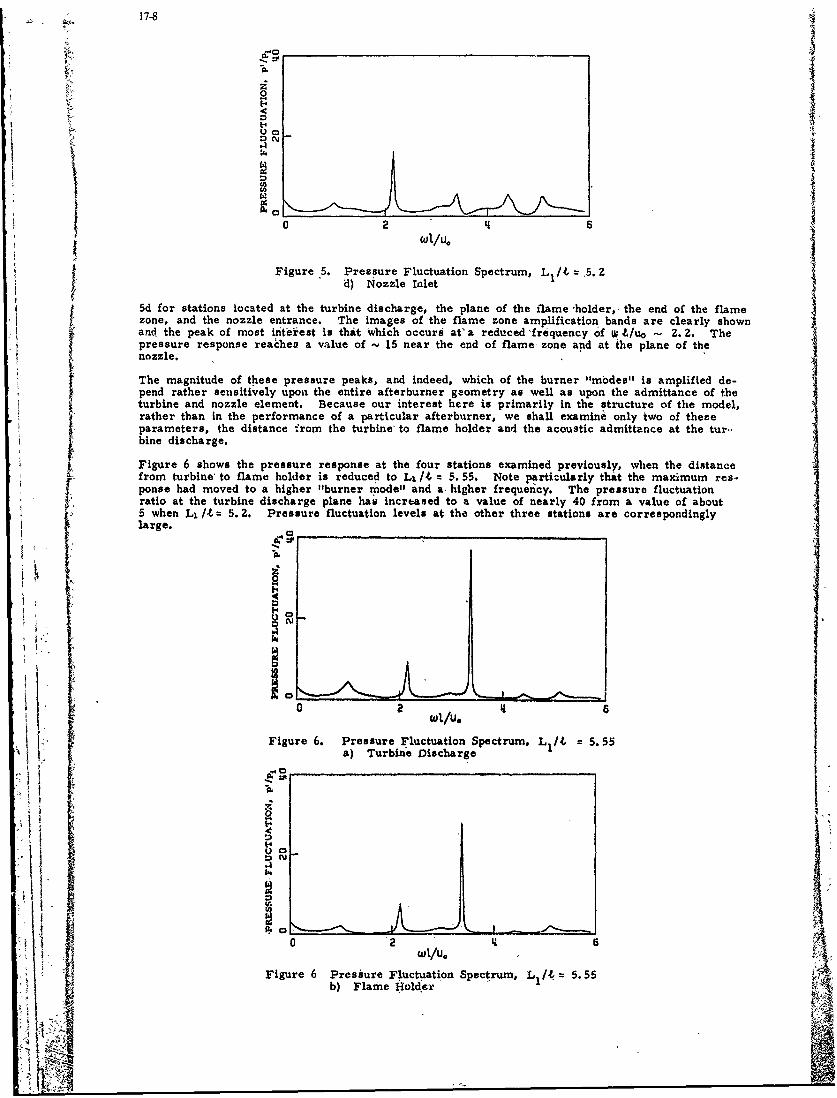
17-8

I-

Co I

U)

02 wIu 6

tWFigure 5. Pressure Fluctuation Spectrum, L 1/4 .5. 2

d) Nozzle Inlet

5d for stations located at the turbine discharge, the plane of the flame 'holder, the end of the flamezone, and the nozzle entrance. The images of the flame zone amplification bands are clearly shownand, the peak of most interest is that Which occurs at'a reduced 'frequency of w 4/uo - 2. 2. Thepressure response reachev a value of - 15 near the end of flame zone and at the plane of thenozzle.

The magnitude of these pressure peaks, and indeed, which of the burner "nmodes 1 is amplified de-pend rather sensitively upon the entire afterburner geometry as well as upon the admittance of theturbine and nozzle element. Because our interest here is primarily in the structure of the model,rather than in the performance of a particular afterburner, we shall examine only two of theseparameters, the distance irom the turbine, to flame holder and the acoustic admittance at the tur..bine discharge.

Figure 6 shows the pressure response at the four stations examined previously, when the distancefrom turbine to flame holder is reduced to Li A = 5. 55. Note particularly that the maximum res-ponse had moved to a higher "burner mode" and a higher frequency. The pressure fluctuationratio at the turbine discharge plane ham increased to a value of nearly 40 from a value of about

0 2 Ii/. 6

Figure 6. Pressure Fluctuation Spectrum, Lthre A 5. 55Sa) Turbine Discharge

V V

_4

Co

A0wi/U.

Figure 6 Pressure Fluctuation Spectrum, LI/J = 5.55b) Flame Iolder

iFI

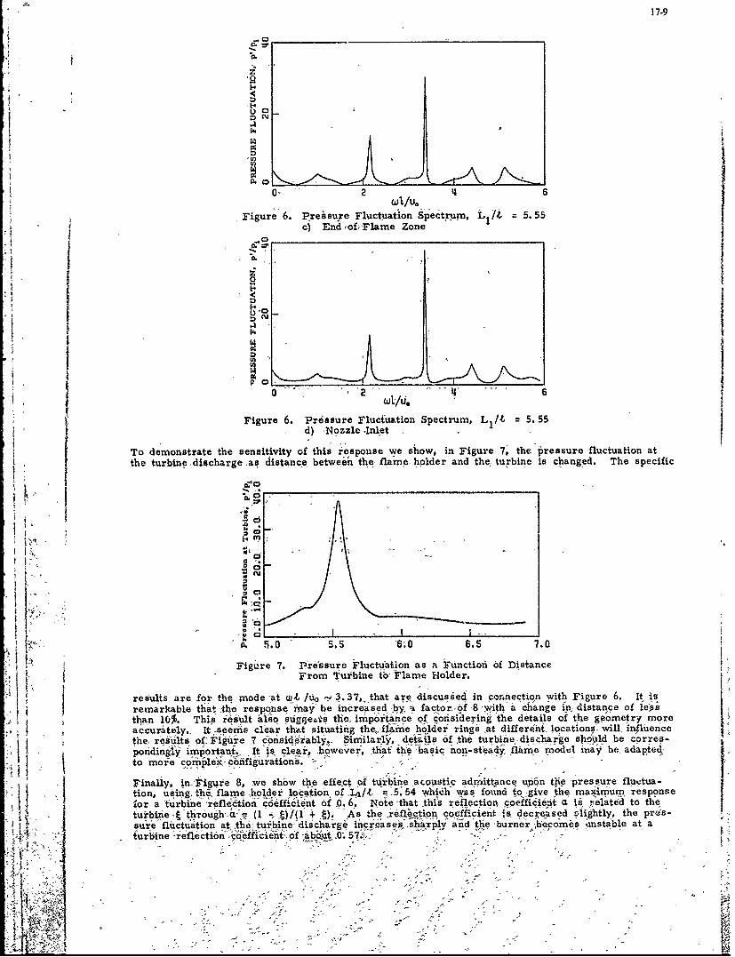
17-9

02 2 6

4Figure 6. Preisure Fluctuation Spectrum, L1 L 5. 55

I *c) End of'F1ame Zone

P0

Figure 6. Pressure Fluctuation Spectrum, L11At 5. 55d) Nozzle -Inlet

To demonstrate the sensitivity of this respoixse we show, in Figure 7. the pressure fluctuation at

Ithe turbine, discharge .as distance. between the flame. holder and the, turbine is changed. The specific

a

444

' .05.5 6.0 6.5 7.0

4 Figure 7. IPre'ssure Fluctuiation as a Functioni of DistanceFrom turbine i'o Flame Holder.

results are for the mode -at 3, 3u #3.7,, that are~ discusied in cnetowihFigure 6. It is

remarkable that -,te espqnse, m~ay b nrese -by -a fator.-of 8 -with a change _n: distance of ie~sth~an 10s. This 46ul ato~geste motne~.~rsiaer'inj-the details of the geometry more

accurately.- It I seems clear that situatin~g thejfiiiie holder rings at differeit.-locations, will, influen .ce

the, results of. Figure 7 considirably., Similarjy, det..ils of th6, turbine-discharge shpuld -be corres-

to more 'ccn-ple~x- co'nfigurations.

Finally, in.' Figure 8,, we show the effect oi turine acoustic adm'ittance upon the~ -press~ure flu.etua-tion, using, the,flame .holder location of Li/k =5. 54 whih w'as foundt to _give &h mna~iimum response

fo atubie efecio cef'cen o 06' Note -that -thi ,s reflection coefficiet is ,elitea to the;o turbine eci -6fiin o 0

'11-' ~ tturbine-, (1.;.~I~ As he reflectin co~ff dent is dec~e~sed slightly, the pres-sure fluctuation at'the -turbine- discharge increasessharply and t~e 'bunrbcms~ntbea

-turbine 'reflection "coeffpiicient' of 'bou 0 '57:",

W.-

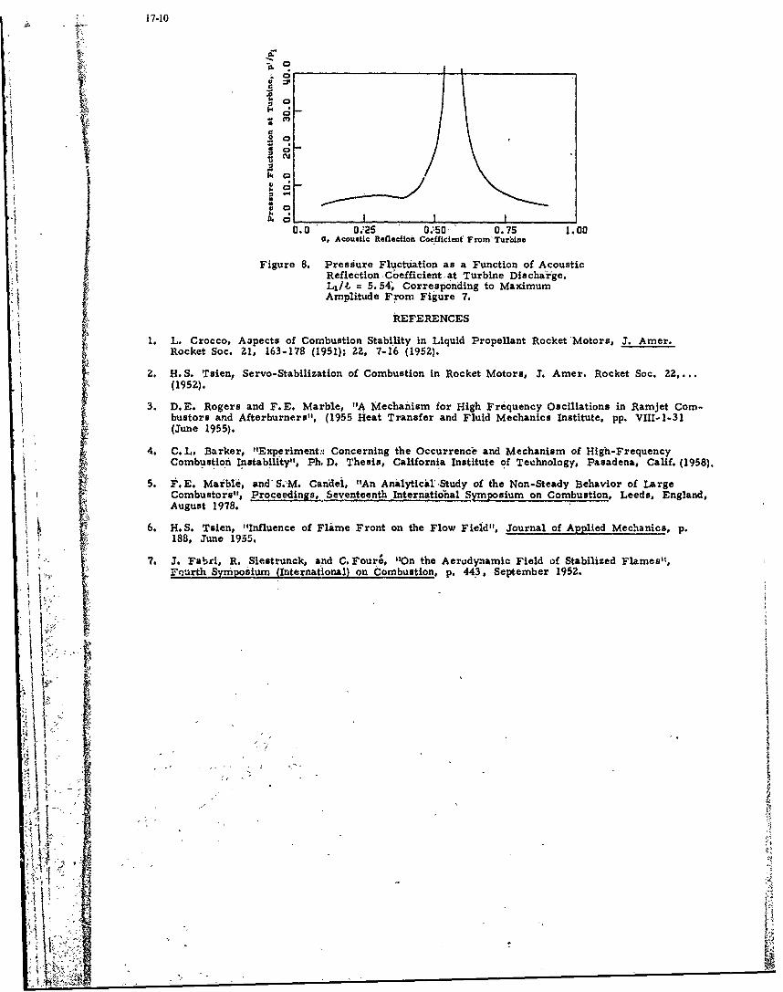
17-10

• 0

0.0 0,25 0 50 0.7S 1.0

G , Acoustic Refledioit CoeIfficient Frorn-Turblne

• Refletion C'Oefficient at Turbine Discharge.Li/t, = 5.54', Correspionding to MaximumSAmplitude From Figure 7.

~REFERENCES1 I. L. Crocco, Aspects of Combustion Stabi ty in Liquid Propellant Rocket Motors, J. Amer.

Rocket Soc. 21, 163-178 (1951); 2 5, 7-16 (1952).

2. HS. Taien, Servo-Stabilization of Combustion in Rocket Motors, J. Amer. Rocket Soc. 22 ....(1952).

3. D.E. Rogers and F.E. Marble, "A Mechanism for High Frequency Oscillations in Ramjet Com-bustors and Afterburners", (1955 Heat Transfer and Fluid Mechanics Institute, pp. VIU-l-31(June 1955).

4. C.L. Barker, "Experiment,. Concerning the Occurrence and Mechanism of High-FrequencyComustion Instability", Ph. D. Thesis, California Institute of Technology, Pasadena, Calif. (1958).

5. F.E. Marble, and S.,M. Candel, "An Analyticil Study of the Non-Steady Behavior of LargeCombustors", Proceedings, Seventeenth International Symposium on Combustion, Leeds, England,August 1978.

6. H.S. Tsien, "Influence of Flame Front on the Flow Field", Journal of Applied Mechanics, p.' 188, June 1935. -7. J. Fabri, R. Siestrunck, and C. Foure, "On the Aerodynamic Field of Stabilized Flames",

.; r'- ~Fourth Syrnposium (International) on Combustion, p. 443, September 1952.

4

. ,

Al

_w/

14

17-11

DISCUSSION

O.K.L.Lee, UK(1) Does the flame-zone considered in your present modelling need to be compact relative to the low oscillatory

frequency?

(2) IF YESWould the solution break down completely if your modelling is applied to smaller scale laboratory burnerswhich, under forced conditions, may have the parameter (I/uo) close to your limitation of 1/4 wavelengthcompactness.

Author's ReplyThe model rests on the assumption that the waves propagating in the duct are plane. This is so if the wavelength islarge compared to the duct width, the flame zone need not be compact relative to the wavelength. An additionalcomment is worth giving. Consider the greatest reduced frequency used in the calculations: wl/u, = 6.

The associated wavelength in the cold stream is then X = I/Mo. For Mo = 0.1 the wavelength is about ten timesthe duct half width (X = 101). If we also assume that the ratio of normal flame speed to free stream velocity iswl/uo = 0.1 then the corresponding flame length is about ten times the duct half width (L = 101). Thus at thegreatest reduced frequency considered in the paper the wavelength is of the order of the flame length and the flamezone is nearly compact.

A.Sotheran, UKYou are saying that the maximum response is when the flame holders are situated at 5D downstream of the turbine.It would be a fairly closed system. In practice when the flame holders are near the turbine it's very difficult to makean after burner. Engines like the TF30, which are close coupled to the turbine have a by-pass stop.

If you imagine a plane wave travelling through the flame front it may cause a transverse pressure gradient, thatexplodes the flame. Is there any possibility of expanding your analysis to include this cross stream effect?

Author's ReplyI think it's possible. We would assume 2 pressure perturbations in the 2 streams. The diffictlty in integraltechnique is that we have to relate those 2 perturbations, maybe by the momentum equation. We don't use themomentum equation in the Y direction: pressures are the 3ame above and below the flame. This equation is ableto accommodate a pressure gradient in the Y direction.

Comment by ASotheran, UKIncidentally, in after burners we see a recovery of the flame, after its collapse, remarkably similar to the filmpresented in the previous lecture (Paper 16 by F.Hirsinger and H.Tichtinsky).

D.K.Hennecke, GeDo you Want to keep your model I-D?

. + Author's Reply

The calculations are indeed performed in the case of a constant area duct. However an extension to the variable areaduct seems possible. The basic integral relations used in the model would have to be slightly modified. As anexample Equation (13) describing mass conservation in region I should be written

aa-pt(l-I -)+p t( I) + w1 secO = 0

where I :FI(x). p, should be allowed to vary with x and similarly p2 would also become a function of x. Twoadditional equations would then be required and might be obtained by considering the balance of energy in regions 1and 2.

As impliedby. Dr Hennecke's question this extension seems worthwhile.

I i '

I .

18-1

SURVEY 0., PREDICTION PROCEDURES FOR THE CALCULATION OF FURNACE PERFORMANCE

by

I.B. MICHEL, S. MICHELFELDER and R. PAYNEInternational Flame Research Foundation

c/o Hoogovens IJmuiden BV §'

Building3,G.19Postbox 10 000

1970 CA IJmuiden/The Netherlands

SUMMARY

The design of a furnace, or more specifically the prediction of the performance of achosen design, can be carried out at several levels of sophistication. Dividing the per-formance of a furnace into separate processes, one can distinguish between fluid flow,mixing, combustion, radiative and convective heat transfer, conduction, noise generation,generation of pollutants, etc. Although it is desirable to understand all these processesfor an optimum design or operation of a furnace/burner combination, in practice it isusually not possible to attain the desired objective due to limitations in time, moneyand knowledge.

Due to this restriction prediction procedures have been developed for separate processesand in this paper it is attempted to classify the numerous published mathematical modelsfor the prediction of furnace heat transfer into three categories. The degree of subdivi-sion chosen for the heat transfer calculations (dimensionality) has been used as maincriterion It is shown that the flow pattern and the desired accuracy determine the re-quired degree of subdivision, which can.be zero dimensional (model type I), one dimensio-nal (model type II) or multi dimensional (model type III). The survey on models and someapplications show also that all model types have their justification and their specificrange of application.

Models of the type I and II are generally considered to be especially suitable for prac-tical furnace calculations and parameter studies. In principle these calculations canalso be performed with models of the type III although their applicability is as yet con-fined to special cases which can be handled computationally and where the greater effortand expense is justified. The latter is fulfilled in cases where data on flow pattern arerequired to decide if models of the type I and'II are applicable, or when the flow dataare needed as inputs and cannot be provided by simple isothermal modelling techniques.Type III models could also be of great value for parametric studies of such quantitieswhose effect on heat transfer and/or other furnace performance data cannot be predictedwith sufficient accuracy by the simpler models.

For typical 3D geometries and if pollution emission data are to be predicted, whichdepend heavily on local properties, the use of type III models is indispensable. However,the use of type III models is unfortunately to date limited in their application to prac-tical situations as some of the conditions met in industrial practice can only be appro-ximated or cannot even be handled computatibnally, i.e. strongly swirling flows, geometryof industrial burners, soot formation and radiation etc.

NOMENCLAURE

A Area, m2

p specific heat at constant pressure, kJ/kg0 K'E black body emissioni W/ml

GG total exchange area between two gasvolumes, m2

GS total exchange area between a gasvolume and a surface element, m2

rs total exchange area between two surfaces, m2

H lower calorific value of fuel, kJ/kg

h enthal py, J/k4 . . .

Jj, Jh m61ebular diffusi6fifluk vector of mj respectively h, kgj/m 2s and kW/m2K, attenliation coefficibnA, in el!

k heat tranisfer coefficient at the wall kW/ni2 OKi L flame length, m

massflow, kg/hmj assc66'centration of chemical species j, kgj/kg

press ure, N/m2

Q heat flowi kW4 hiat flow density, kW/m

2

qstr abs6rbed radiative energy per unit Volume and time, kW/m3

Ri production rate of m; per unit Volume and time, kgj/m3.s

Tt temperatu re OK and'O~TV shear stress tensor, N/m2

V 46svolumex,y'z cartesiia co"0rdinates

onvectiVe heat tiansfer coefficient kWl/m 2 OK

A difference between two values

S) Formerly director of the Research Station at IJamiden; presently employed bySteinrdller GbH, Gunersbach/Geimany

18-2

e emissivityn furnace efficiencyP density, kg/m

3

dimensionless stream functioivelocity vector, m/s

The quantities of equation (8 - 11), which are marked with , represent averaged respec-tively fluctuating quantities. The sign 6 stands for a tensor multiplication.

INDICES

a airf fuelG gasjet forward gas flowi,j,k,lcharacterization of gas and furnace elements, running numberin entering gas flownet net exchangeout leaving gas flowr recirculating flow

U ambientW wall, heat sink

1. INTRODUCTION

The vast amount of money involved in the combustion of fossil fuels in industrialfurnaces has for many years stimulated efforts to optimize furnace performance. Asthe achievement of this goal via large scale experiments on individual furnaces isexpensive and therefore undesirable, attempts have been made to develop mathematicalprediction procedures for furnace heat transfer for almost half a century. The inabi-lity to accurately describe the complex interactions of the physical transport pheno-mena and the chemical reactions within industrial conibustion chambers prevents how-ever an exact mathematical solution of furnace'heat transfer. This resulted in thedevelopment and publication of a great number of mathematical models with differentrestrictions and limitations as the selection of the necessary assumptions and appro-ximations is generally based on specific conditions. The large number of models andtheir indi'vidual range of applicability. often makes it difficult to decide which mo-del: is best suited to a particular purpose. To some extent these difficulties can beovercome when the models are classified into various groups, characterized by welldefined specific tiitations and applicationl ranges. To give such a classification isthe objective of this paper.

The testing and furt:her development of procedures to predict furnace heat transferhas bee6n one of the major research lines at the Research Station of the IFRF in re-cent years (1971-1977)*.and the close contact with many different approaches lead to aclassification of the models into three basically different types. These model typesdiffer both in their degree of complexity and the information wbich can be obtainedfrom their application:

* Type I tzerc. dimensional modelsModels for th., prediction of an averaged furnace heat transfer, the furnace effi-ciency, and other averaged properties

* Type II : one dimensional modelsModels which allow the prediction of an one dimensional heat flow d(itribution andother properties. Mostly as representative dimension the furnace (flame) axis ischosen.

* Type III: mwilti dimensional (2D, 3D)" mdeisModels which allow the deteirmination of the spatial distribution of heat flow andother pr:opertieS. Cylindrical 'furnaces can be dealt with by 6omparativ'ly simpletwo dimeasiofiil (2D) proed~ces, whereas' most industrial furnaces require a threedimensional approach.

In spite of the-substantial differenceg between many of the mathematical furnace mo-Cals described in the literature, m't axibe classified under one of the three~~~groups (model types) mentioiieda'bov&. ....Inghoptdr 2 the main features of the various model types and the approacheb used at

the Research Station are discussedi

2. MATHEMATICAL MODELS FOR THE- PREDfCTiON OF FURNACE HEAT TRANSFER

All three model types can serve the same basic goal, thepiedintion of furnace per-formance from known input ahd'bou dary conditions. Final objectives nay however bevery different, firstliby nature-e.4y. for fundamental research 6r inddistrial appli-cation, and secondly f6r their major field of interest e aerodynamics, heat trans-fer, flame mechanisms.

AS far as fundamental research is concerned, modelling techniques can generally besimplified either-from theo6etical hJthess or from the particular design of a tez-

oo'°a model becomesk therefore a rther 6;sy task. However, in the field of industrial

dpplication a model is expected to yield comprehensive information with less time andat less cost than large scale experiments as a means to improve furnace, burners orprocess design. The following will mainly be concerned with industrial furnace modelswhere emphasis is given to heat transfer performance. Information required as input

t and obtainable as output for the three model types is given on fig. 1.

General information to be Additional specific information Information to be obtained,specified before calcula- required, dependingon model type depending on model typetion

A. Input conditions TYPE I - UNIFORM FLOW FIELDa fowsAverage values of gas temperatureass flows, Average convective heat transfer (Ta), wall-and charge temperature!enthalpy flow (T) al-fndchrg tmpraurlp a cefficient (TW), heat flow to wall aid charge

fuel and air (W) and furnace efficiencycomposition

B. Boundary conditions TYPE II - UNIDIRECTIONAL FLOW FIELD

Geometry, conducti- 'Macro flow pattern (forward and re- Same as type I, but additionallyvity and emissivity circulating gas flow), axial decay one dimensional distribution ofof furnace wall and 1 of che.iical energy, local convective gas (TG) and wall temperature (TW)charge heat tr i sfc. coefficient and heat flow density

C. Radiative constants TYPE III - MULTIDIRECTIONAL FLOW 'FIELDGas emission and Complete flow pattern and spaial gas Sama as type , but additionally

1 absorption data de-pendingion da d- fconcentrations, turbulent exchange complete spacial distribution ofpending on radia- coefficient for heat, local convective gas (TG) and wall temperature (TW)tive submodel heat transfer coefficient and heat flow density

Fig. I : The information required for and obtained from the calculation of furnace heat transferwith the model types I to III; the various specific information can be provided frommeasurements or mathematical submodel. .

The detail in the input and output information can be seen to increase from nodeltype I to type III, and is accompanied' by an increase in the degree of subdivision ofthe furnace under consideration into-more and more elements as shown in fig. 2.

TYPE I TYPE II

_YP III<4/ tol 0 ( harse)/] I

" eat flowdistributj fr ' j

heat flow distribution

Fig. 2 Thedegreeof-subdivisionrequired for a rectangular furnace - and the heat flow distribu-tion-0b'tained -in'.dependency of the model type to be'applied.

The representative model types I,,- I and- *II usedat the IFRF are all based on thewell-known Zone Method devel6ped by Hottel et al.Ll] for the calculation of radiativeheat transfer In, enclosures.

2.1, Model, type I (zgdro dimensional model, ,fig. 2, -type.-I)

'The determination Of- the -distributioh of. the heat flow density over the surface oftheo stock is desirable .and sornetimes necessary,,althofuh a propar orienting firststep which.6ten suiffices is the determiination of ,the total heat transfer as a func-tion of fruel iid ,ir inputs Even if -t is he, sole Objective, knowledge of the de-tailed interacrtion 'Of radiation- and;.c6nvction- wiyh, mass transf 6r -and copbustibn isil principle,,necessary. ,,H6weved, integral formulations are t6lerant of casual treat-ment of detail, especially in the presence of the levelling

urpri'singpesenc e~~' vrll eeln ffect of radiation,, and.asurprisi y g accuate ov'erall performtan'e is predictable fr6nj a, relatively simple

A zero dimensional model does, not take accouit of length- and timeVdimensions within,[the' furna'e. In such a 6ode gradients of quantities like velocities, temperatures,

184

heat flux densities etc. are neglected in all three co-ordinate directions, which im-plies that all these properties are considered to be uniform. The model is thus basedupon the assumption that the processes inside the combustio.n chamber can be describedwith a reasonable accuracy by one representative average value for

- combustion pattern;- gas temperature;- temperatures of the heat sinks;- gas concentrations;- soot particle concentrations;- radiation characteristics;- convective heat transfer to the sinks;

similar to the processes in an ideal well stirred reactor.

For many years such models have been used for the design of radiant cells of boilers,furnacbs of the petrochemical and other industries. Well documented examples of zerodimensional models have been published by Hottel and Sarofim F|i , Jeschar and SchupeL2] and Hotte' [31. Major differences between the numerous models to be found in lite-rature are the treatment of:

- the radiative exchange between gas-, walls- and beat sinks (stock) within the fur-nace (e.g. gray or non-gray gas radiation) an

- the furnace walls, either adiabatic or with wall losses.

Although a truly zero dimensional situation cannot exist in practice and the accuracyof the predicted results depends n the degree of deviation from zero dimensionalityof the furnace/burner system under consideration, these models can predict the righttrends for the effect of operational variables on the overall furnace perform;.rce inmost cases, i.e. the effect of:

- adiabatic flame temperature (fuel type);- heat sink temperature;- firing rate;- heat loss through walls;- excess air;- air preheat;- oxygen enrichment, etc.

Large deviations from the assumed well stirred conditions upon which the model isbased, can cause substantial discrepancies between the real and the calculated overall

*efficiency. For long furnaces with a small cross-section (no gas recirculation) andcold walls, fired by a short flame, the overall efficiency can be underpredicted by

* more than' 20% (flame D.2.2, ref _38). overpredictions of the same order of magniitudehave to be envisaged When the model is applied to long narrow flames in a comparative-ly wide combstion chamber (flame 29, ref. [34J).The Re',Larch Station's model type I, used also for the predictions discussed in chap-ter 3.1, is a modified version of the rdel described explicitly in L3-. Major changesadopted are the inclusion of wall losses and a non-gray gas radation model. For eachof the'heat sinks i (fig. 2, furnace hearth, sidew:ll, roof) and for the gas volume,energy balances are drawn up:

heat sinks i

G1 EG + EjSjSiE- Ai iEi + Ai i(TG - Tw,i) = Aiki(Tw,i - TU) (1)

arriving'radia- off radi- net convective net heat flowtiie heat flux ation hdat'fl6w

GGEG + GSGE 4KVGE A-ji(TG - T -) + *FlH + C 6(Ti - TG) = 0 (2)

arriving radla- off kadi- net convective latent enthalpy flowtive heat flux aticn heat flow heat

A detailed-description of the derivation of the total exchange areas GG, GS and SS can:)be found in l1,4,51. The' solution of these non-linear algebraic equations yields theCverage temperatures of the heat sinks (TW) 'and the gas volume (TG) as well as theheat flowis 'to all heat'sinks i considered within the furnace.

t -Model type,.U '(one- dimensional 0odel, fig. 21i type II)

1 ! Wher the combustion system under considc ration deviates strongly from the well stirredasmp ioi, the heat flow distribution .'.'i loose its unif.rmity. Although adjustmentscan be madedin rder to cdlibrate_the zero dimensional- modelsoto enable the determina-tion of an overall effidiency'-in such cases, they can never give information on thediptribution of thheahaflux density over the stock, respectively the heat sink. Thisli'er informition is-h6wever req!lired under circumstances where the heat flow densi-j 7 ie ave-to be keptin: beteeh certain'limits, i.e. because of the danger of overhea-

Stin 6f1 thichdgeor of hazard to he',planti Toobtain n6re detailed informatin ispossible only by the ihntr6ductioi 'of .Idimensions" like -t.me and length.' hIn ,anY furnaces thd heat flow density varies dominantly in ohe dlrection, which isg rlyth a flodire on In this asi is often~suffizient to introduce

Sa'only'length dmnesibn to' alow the determination of the most important heat flow andte ertue istibtion. The prediction procedure then becomes a one dimensional mo-del, an ilius example of which is shown on the centreof fig. 2.

In one dimensional furnace models generally only one length dimension is taken irtoaccount. Gradients of the different quantities in the two other co-ordinate directionsare neglected. This implies that the velocities, temperatures etc. are assumed to beuniform in finite cross-sections along the main co-ordinate direction. Furnaces forwhich this assumption is reasonable are usually long in comparison to their width asin such furnaces the gradients perpendicular to the length dimension are often ofrainor importance. As shown in chapter 3.2 the application range of one-dimensionalmodels can be extended also to rever'eratory type furnaces (length to diameter ratiosmall) when the latter assumption is modified, i.e. when the recirculating gas flowsare taken into account. Of course the information on the flow pattern required as in-put to the model calculations increases with increasing complexity of the adopted flow

The subdivision of the furnace into a sequence of individual sections does not cause afundamental change in the calculation procedure, only the number of equations increa-ses Cs for all individual elements in a section balance equations have to be drawn up.Each section can be treated in a way similar to the procedure described in chapter

The main differences encountered in published work on one-dimensional furnace modelsare in the, treatment of radiative heat exchange and the assumptions of the idealizedflow pattern adopted in the models.

The most well-known type II model is the so-called long furnace model after Hottel andSarofim [1]. Some of the major assumiptions made are: no recirculation of gases in thefurnace, combustion completed at the burner exit, no net radiative exchange in maingas flow direction.

Seluk et al. [67 assume also a plug flow pattern (i.e. uniform "forward" velocity,temperature and species concentration at any cross-section), whilst taking accountof radiative inteichahge between different locations in the main flow direction andallowing for a gradual "stepwise" chemical heat release along the flame axis.

In situations where the real flow pattG,:n is not approximated by the plug flow con-cept, e.g. with the apprearance of substantial recirculation zones in the combustionchamber, the plug flow assumption leads to an overprediction of heat flow density, es-

j pecially at locations where cons±derable heat release occurs. Some type II modelsallow account to be taken of gas recirculation zones, when these are confined to theburner near region, by using a well stirred plug flow conc(pt for the description ofthe flow pattern. Here the burner near section is treated as well stirred, the succes-sive sections as plug flow. The length of the well-stirred section is usually chosen

j to cover the area from the burner inlet to the point of impingement at the wall, i.e.the part where recirculation occurs. Models of this type have bee, suggested by

J Michelfelder and Lowes [51, Lucas and Lockett [7] and Clement C8].fhe application of this idealized flow pattern description is obviously not suitablefor furnaces in which the recirculation zone stretches over the entire furnace lengthor covers the major part of the furnace (heaters in chemical industry, reverberatoryfurnaces etc.). To determine a heat flow distribution n such furnaces requires a morerealistic description of the flow pattern, i.e. a masz interchange in forward andbackward direction between adjacent sections has to be considered. At the IFRF a modelhas been developed [10 3 which allows account to be taken of gas recirculation by usingthe flow pattern model shown on fig. 3.

'1er,in rure,2011nt "r,2,in " e,3t to

~~G~r

Fig FIk pattern model gsted fof the determinatioa of an one-dimensional heat tdow distri-

As indicated on this figure the fl6w is separated into, a forward and a recirculation-regionwith different temperatures., Although the radiation exchange is calculated with

mean" Section 4- te £ature '(one--dikis ionai'modbl) a pseudo two-dimeasional treat-4ment of the flow is introduced by relating the'mean radiation temperature to the re-'>' ..2 i Crculation- (Tr ) ',ard jet-temperature (Te."

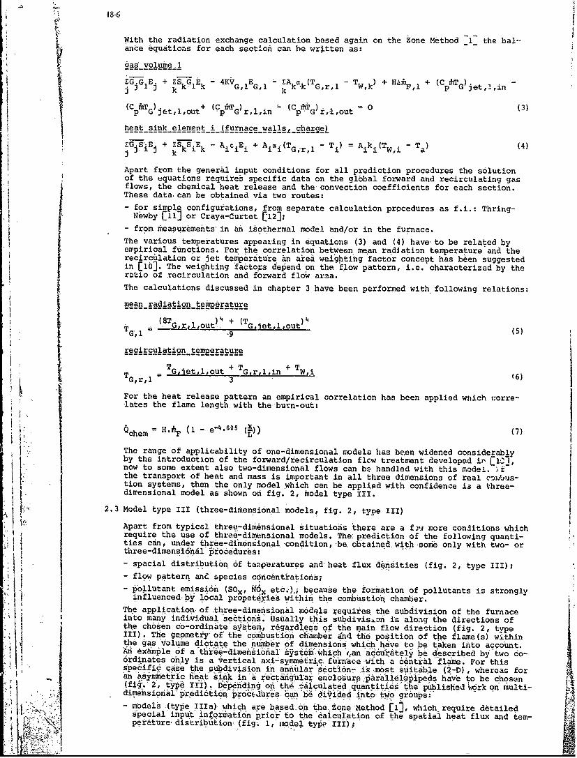
18-6

With the radiation exchange calculation based again on the Zone Method -I- the bal-ance equations for each sectioi can be written as:

&as volume 1

jG G E + -Gitk 4KVG'EG' EA (T TK +,~ TWk) l + (CpffiT G1G EZ Gl Gl k Grl W p G jet,1,ink k

(C p nG) jet,1,out + ('pmTG) r,l,in (Cp AG) r,l,out = 0 (3)

heat sink element i (furnace wais._c2harge)

ZG S'-E + ZSS'E - AiE + A a-(T - Ti) = Aiki(Tw, i - Ta ) (4)k k 1 iki Gir,l ai~ a4

Apart from the general input conditions for all prediction procedures the solutionof the equations requires specific data on the global forward and recirculating gasflows, the chemical heat release and the- convection coefficients for each section.These data can be obtained via two routes:- for simplq configurations, from separate calculation procedures as f.i.: Thring-Newby Cll3 or Craya-Curtet [12];

- from measuremeits in An isothermal model and/or in the furnace.The various temperatures appearing in equations (3) and (4) have to be related byempirical functions. For the correlation between mean radiation temperature and therecirculation or jet temperature an area weighting 'factor concept has been suggestedin [10]. The weighting factors depend on the flow pattern, i.e. characterized by theratio of recirculation and forward flow araa.The calculations discussed in chapter 3 have been performed with following relations:

mean radiation teftodrature

(8TG,r,l,out. + (TG,jetjl,out)5TG, 19

recirculation temnerature

TG,jettlfout + TGrlin + TW(iT Gfr,1= 3 (6)

For the heat release pattern an empirical correlation has been applied wilich c:orre-lates the flame length with the'bu.n-out:

chem H.A (1 - e -4 . 60 5 (L)) (7)

. The range of applicability of one-dimensional models has been widened considerablyby the introduction of the forward/recirculation flcw treatment developed in CicJ1,now to some extent also two-dimensional flows can be handled with this model. *fzthe transport of heat and mass is important in all three dimensions of real coi.\bus-tion systems, then the only model which can be applied with confidence ia a three-dimensional model as shown on fig. 2, model type III.

2.3 Model type III (three-dimensional models, fig. 2, type III)

Apart from typical three-dim nsional situations there are a f.ni more conditions which~require the use of three-dimensional models. The prediction of the following quanti-ties can, under three-di mensional condition, -be, obtained, with some only with two- orthree-dimensihal & odure: .

- spacial distribution of tenpLaratures and' heat flux densities (fig. 2, type III);- flow pattern ane species concentrations;- pollutant emission (SOX, N 6x etc.) -because the formation of pollutants is strongly

influenced- by local propeteries within the combustio' chamber.The application-of three-dimensional models requires the subdivision of the furnaceinto many indi.vidual Section6.' Usually- tis subdivision is along the directions ofthe chosen C-ordina te'slstem, regardles's of the main flow direction (fig. 2, typeIII) . -The geometry of' the combustion Chanber and the position of the flame(s) withinSthe gas Volume dictate the number of dimensions which have to be taken into account.4A example of a tfiiee-'dimen~'1i a 'li ys tem which ,an a ccu rately- be' d es cribed by 'w " o6rdinates only is a vertical axi-symmeric, furnice with 'a 6entral flame. For thisspeific case the subdivision in annular secti6n - is most suitable (2-D), whereas forSan 9symeic eat siik in a zeCtugular enclosure paralieleppeds have to be chosenig. 2, type III). Depending on the calculated quantities the published work on multi-I : . dimehsionalo prediction pr6cdhrescan divided intot o groups:models (type IIIa) which are based-0n the .one Method [l, which require detailed

n~l'<> ! Special input information prior - to the 'calculation of the spatial heat flux and tem-xpeiature ..... dis'tribtion (fig ' 1,nodel' typ III ) ;.

~18-7

- models (type IIIb) which are based on the numerical solution of the convectivetransport equations, the solution of which yields information on the spacial dis-tribution of all properties. Similarly to the model type I only the general inputsdescribed on fig. 1 are required'for the application of this model.

2.3.1 Three-dimensional models based on the Zone Method of analysis (type IIIa)For this model type energy balances are formulated 'for all the elements of thesubsections similar to the model type II. The only basic difference betweenmodel types II and Ila is that for the latter the energy and mass transportbetween gas volumes is no more c6nfined to one direction. As for the modeltype I and type II total exchange areas have to be -determined from so-calleddirect exchange areas which are available for two different geometries in [I],in graphical form for cubes and tabulated for annular sections (axi-symmetricsystems).

calculating direct exchange areas for annular sections of rectangular cross-

section, with different attenuation coefficients in the various sections.

Models based on the Zone Method have been applied successfully to the calcula-tion of the spatial heat flow distribution in different types of combustionchambers [14-16]. Of special interest to IFRF members are the applications ofthe Zone Method approach to the Nr. 1 furnace of the Research Station[4, 181.A major shortcoming of the model type IiIa, is the large amount oi detailed in.-put data required on flow, mixing andchemical heat release before the solutionprocedure for -the determination of the heat transfer can be started (fig. 1).Global assumptions similar to those made for the 'model type II are not suitablefor model type Ilia, as the, accuracy of the prediction depends heavily on thequality of the input data. The specific inputs can be obtained in enough detailonly from isothermal models or-predictions from models of type IlIb.Furthermore it is virtually impossible to correctly incorporate the slmultane-ous dependency of the attenuation coefficient on the local gas temperature andthe temperature of the radiation source within the conventional Zone Method.This can however be overcome by the application of the Monte Carlo Method forthe calculation of direct or total exchange areas, Published examples of thismethod call be found in E13, 19, 20].

2.3.2 Models which are based on the numerical solution of the convective transportequations (type IIlb)With the model type IIIa energy balance equations are solved to predict spatial

heat flux and temperature distributions. Before the model can be used detailedinformation on the flow and concentration field is requiried as input, If thedetermination of these properties should be included in the prediction proce-dure, then equations describing the transport of species and momentum are t.i beincluded. Models of the type IIIb are capable of doing so as they are derivedfrom the basic differential equations which describe the exchange of a] timeaveraged properties. For a quasi'stationary flow and with some slmplificationsthese equations can be'written in vector form as:

Continuity equation : div(0i-) = 0 (8)

Transport of momentum : .div(p o-) + div(pw o i) - grad p + divr (9)Transport of species : div( m .'+ j) + div( m.) R (10)

Transport of energy : div(ph + Jhl) + div(ph ) qstr (11)

The numerica]. procedure for the solution of equations (8 - 11) involves thesetting-uo of an orthogonal computational grid to cover tt,-i flow field and thespecifidation of boundary conditions along the flow field Lboundaries. The gridnodes represent centres of small volume eleements over which the diflerentialeqlations are numerically- integrated. Sc 1- 'n procedures have been published bySpalding'[21] for axi-symmetric (Z-D) ayr. -az and by Zuber [22_ for thzee-dimensional systems. Models of the type IK:b nave been used with-some success-by Michelfelder.et al." r41, Gibson and Morjan C231, Lowes et al.L24J andRichter-et al., E25-27.

In trying to applymodels of the type IiIb to, combustion systems one has tofade seve'ral I kincilee-p I iems9 The physicalrelevaceof- thie solution of the flow equation depends strongl

on -the correlation term6s for the- turbulent properties _o ou, pm!w' ahd -ph'',which describe the ihceease -of momentum-, species- and enthalpy 2transport.dueto turbulent exchange. A number of turbulence models have, been suggested F281.It is hovever -StftI'necer-aiy to "calibrate" the empirical constants 6f theseielationsto the flow problem under.conSideration."-Recent investigations atthe Research Stati6 [29] indicated,-tlhi the so-called kW model L30] can beu~ed with good confidence for eneiosed-n6n-swiriing double concentric jets.

e The impqrtance of radiative exchange in furnaces and the difference in naturebetween the tra-sport'of the other'quanitit±es - mass, momentuim, species andenthalpy - 'viich can accurately be described by differential equations and -

radiation which, due to idinteg nature, can only be approximated by dif-ferential equations, introduces another principle problem for type 11b,m d6 f..ep ie b o e.

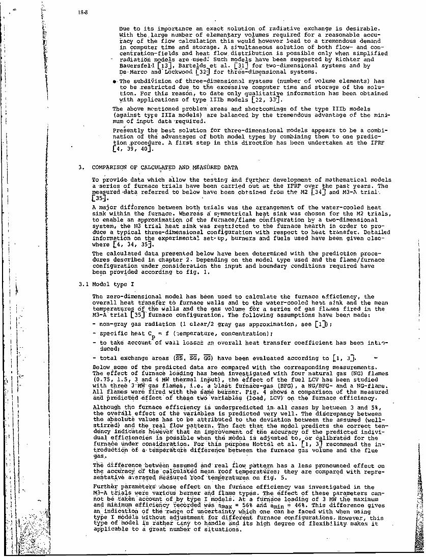
18-8

Due to its importance an exact solution of radiative exchange is desirable.With the,large number of elementary volumes required for a reasonable accu-iacy of the flow calculation this would however lead to a tremendous demandin computer time and storage. A simultaneous solution of both flow- and con-centration-fields and heat flowdistribution is possible only when simplifiedradiation models are used' Such models have been suggested by Richter andBauersfeld [13], Bartelds et al. [311 for two-dimensional systems and byDe-Marco andLockwood F321 for three:dimensional systems.

*-The subdi'ision of three-dimensional systems (number of volume elements) hasto be restricted due to the excessive computer time and storage of the solu-tion. For this reason, to date only qualitative information has been obtainedwith applications of type lIIb models [22, 33].

The above mentioned problem areas and shortcomings of the type IIIb models(against type Ilia models) are balanced by the tremendous advantage of the mini-mum of input data -required.

Presently the best solution for three-dimensional models appears to be a combi-nation of the advantages of both model types by combining them to one predic-tion procedure. A first step in this direction has been undertaken at the IFRF[4, 39, 40].

3. COMPARISON OF CALCULATED AND MEASORED DATA

To provide data which allow the testing &nd further development of mathematical modelsa series of furnace trials have been carried out at the IFRF over the past years. Themeasured data referred to below have been obtained from the M2 f34] and M3-A trial--[35].A major difference between both trials was the arrangement of the water-cooled heatsink within the furnace. Whereas a symmetrical heat sink was chosen for the M2 trials,to enable an approximation of the fucnace/flame chnfiguration byr a two-dimensionalsystem, the M3 trial heat sink was restricted to the furnace hearth in order to pro-duce a typical three-dimensional configuration with respect to heat transfer. Detailedinformation on the experimental set-up, burners and fuels used have been given else-where [4, 34, 35].

The calculated data presented below have been determined with the prediction proce-dures described in chapter 2. Depending on the model type used and the flame/furnaceconfiguration under consideration the input and boundary conditions required havebeen provided according to fig. 1.

3.1 Model type I

The zero-dimensional model has been used to calculate the furnace efficiency, the

overall heat transfer to furnace walls and to the water-cooled heat sink and the meantemperatures of the walls and the gas volume for a series of gas flaes fired in thej> M3-A trial [35]'furnace configuration. The following assumptions have been made:

- non-gray gas radiation (I clear/2 gray gas approximation, see [1-);

- specific heat CD = f (.emperature, concentration);- to take account of wall iossct- an overall heat transfer coefficient has been intio-

, duced;

- total exchange areas (S, SG, GG) have been evaluated according to [I, 3]. -

Below some of the predicted data are compared with the corresponding measurements.ti The effect of furnace loading has been investigated with four natural gas (NG) fldmes

(0.75, 1.5, 3 and 4 MW thermal input), the effect of the fuel LCV has been studiedwith three 3*MWgas flames, i.e. a llast furnace-gas (BFG), a NG/BFG- and a NG-flame.All flames were fifred with the same buriner. Fig. 4 shows a comparison of the measuredand rddictd effect of these two6variables (load, LCV) on the furnace efficiency.

Although tho furnace-efficiency is underpredicted in all cases by betueen 3 and 5%,the overall effect of the Variables is predicted very well. The discrepancy betweenthe absolute values has to be attributed to the deviation between the assumed (well-stirred) and the real flow pattern. The fact that the model predicts the correct ten-

indi6ates howevr that in imprbvement of the accuracy of the predicted indivi-dual efficiencies is possible when the model is adjusted to, or calibrated for thefurnace under consid-ration. For this purose Hottel et al. [1, 31 recommend the in-iroducti&n of a tdmbratarb differeice between the furnace gas volume and the fluegas,.The difference betwben assumed and real flow pattern has a less pronounced effect onthe accuracy of the'ca 6ulA£d mean ro6f temperatuies; they are compared with repre-sental.ve aeraged miaured Yoof :tdmeratuies on fig. 5.Further p~ramete's whose effect on the furnace efficiency was investigated in theM3-A trials were various burner and flame types. The effect of these parameters can-not be takn'account of by-pe Iiodels. At a furnlce loading of 3 MW the maximumand-mihimum efficiency -ec6rded Wasiax = 56% afid' mjn 46%. This difference givesan indication°6f the rauie of uncertainty which one can be faced with when usingtype I mbddl without adjustment for different furnace'configuratibns. However, thistype of'model is rather casy to handle 'nd its high degree of flexibility wakes itapplicable to a great number of situations.ihY,

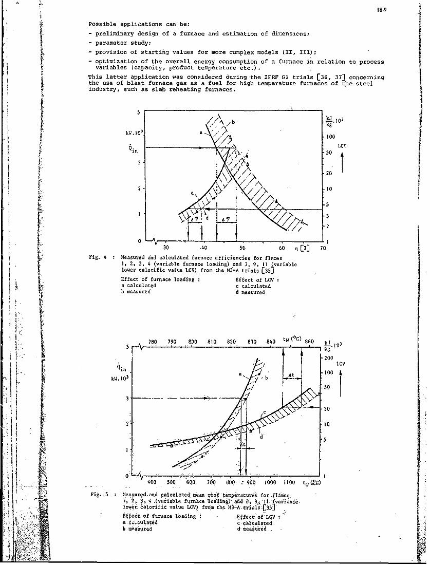
18-9

Possible applications can be:

- preliminary design of a furnace and estimation of diiensions;- parameter study;- provision of starting values for more complex models (II, III);

- optimization of the overall energy consumption of a furnace in relation to processvariables (capacity, product temperature etc.).

This latter application was considered during-the IFRF G1 trials [36, 371 concerningthe use of blast furnace gas as a fuel for high temperature furnaces of the steelindustry, such as slab reheating furnaces.

I k0

LCVin i50

2' 30v m 20

2, ,,o

[* [% 70.2

30 , 060 CI ] 70

Fig. 4: Measured and calculated furnace efficiencies for flames1, 2, 3, 4 (variable furnace loading) and 3, 9, 1I ivariablelower calorific vaiue LCV) from the M3-A trials [35J

Effect of furnace loading: Effect of LCVa calculated c calculatedb masured' d measured

-'2 0 0 C

H IkW. IO3 b

50

3 Xt

-220

2 :1

fa '4 _ A00 '500 -6QO 70'0 6W: 90Q 1000 1100 tw ( m)

Fig .5 Measurd.nd calculatedmea .roof temperturdi for flames,

iowef.icalorifid value LCV) from the M32- trials ,[35 '

"Effect, of funiace. loading j Effec t'of'LCV:,a° ddculatdd c alculate

18.10

3.2 Model type II

The type II model described by the equations (3-7) ha3 the widest range of applicabi-lity of all type II models mentioned in chapter 2.2. If however flow pattern can beapproximated by simple assumptions, other type II models like the long furnace modelfI1 or the well-stirred plugflow approach can yield excellent results. The importance

of-the flow pattern/model combination is shown at the example ofrtwo (natural gas)flame/furnace configurations, i.e.:

- flame D.2.2 fired in the Delft vertical water-cooled furnace (0.9 m diameter, 5 mlength; see [38], and

flame 29 (M2 trials, F341) fired in the IFRF furnace Nr. 1 (2 x 2 m cross-section,6.25 m length).

Flame D.2.2 was a strongly swirling wide flame fired in a rather narrow furnace(L/D , 5,5). The external recirculation was due to the confined situation limited tothe burner near region. This configuration is almost ideal for the well-stirred plugflow approach.

Flame 29, however, was a narrow non-swirling jet flame fired in a rather wide furnace(L/D -, 3) with an external recirculation over the entire furnace length.

The heat flux distribution for both flames has been calculated with the well-stirredplug flow model of the IFRF [5, 93. For flame 29 a second calculation was performedwith the model described by the equations (3-7) [IOl.As shown on fig. F the predi-:tions obtained from the well-stirred plug flow model areexcellent for flame D.2.2. The calculation was carried out with assumptions similarto those made for model type I and following special input data:

- burn-out completed within first section;

- first two sections well-stirred, all following sections plug flow;

- convective heat transfer coefficients as measured in the furnace [383.

200 - -

--- exferiments- predictions

150 -' '.---- -

0 I2 3 4 5furnace length (m)

Fig. 6 : Measured and predicted heat fluw distributions to the water-cooledfurnace walls of the Delft furnace (flame D.2.2, [38])

Using the same approach for the calculation of the heat flow distribution from flame

29 resulted in a complete misprediction In comparison to the measurements the localheat flow predictions were up to 100% too high and at the rear of the furnace 50% toolow (fig.7). The misprediction has mainly to be attributed to the wrong assumption ofthe flow pattern. For furnace configurations which result in similar flow pattern asii flame 29 (most reverberatory furnaces) the recirculation has to be taken account of.With the "recirculation" model [i03 a second calculation has been performed usingfollowing inputs:

- chemical heat release as determined by equation (7) from the visible flame length;

- information on flow pattern (fig.3) obtained from an isothermal physical model;

o , -convective heat transfer coefficients obtained from isothermal model.

As can be seen from fig. 7, curve b, the prediction with the "recirculation" modelis reasonable. This proves that with only a rough incorporation (pseudo 2D descrip-tion) of the real flow pattern the applicability of one-dimensional models can be

extended o situations with two-dimensional flow fields. This type of model is thuswell-suited to long furnaces'and'strongly unidirectional processes e.g. rotary kilns,glass smelters, refinery process heaters and steel reheating furnaces.

Absolute predictions are generally accurate enough to help in the design or modifica-tion of an industrial furnace (heat sink geometry, position and distribution of heat

~18-I1

along the process length). The exercise of selecting adequate submodels viz. for flameradiation of heat release, requires however a good knowledge and experience of theapplication of interest.

Moreover, in most test rigs for liquid or solid fuel characterization, which are oftendesigned to be mono-dimensional, such a heat transfer model can be linked with a simi-lar kinetic model and become an efficient tool for research.

300_ _

4net

200r L.: _

, '

'0 0-i- - - ]300 --------

,

IIi0 1 2

Fig. 7 :Measured and predicted heat flow distribution from flame 29 [34].

a - measuredb - predicted with "recirculation" model [101c - predicted with well-stirred plug flow model £9]

3.3 Model type III

In respect to the calculation of flow and gas concentration fields multi-dimensionalmodels (type IIIb) are still in the development stage. For this reason their applica-tion is usually limited as yet to symmetrical (2-D) systems. In [4] a first applica-tion of a combination of the type lia and type IIIb models has been reported upon.Because of its well-defined flow pattern flame 29 £34] had been chosen for this testtoo.

Discrepancies found between the measured and predicted flow pattern had been attri-buted to the oversimplifying ad hoc turbulence model used. This turbulence model has

!V" now been replaced by the better suited kW model [29, 303. The former calculationshave now been repeated with the following assumptions:

- the rectangular furnace Nr. I has been approximated by n equivalent cylinder;

- chemical heat release is determined by mixed = burnt;

- gray gas radiation with K,=0.1.5 m-I;

- two flux radiation model F13];-convective heat transfer coetficient as measured in isothermal model (same aschapter 3.2).

On fig. 8 the calculated flow pattern is plotted, against the measured stream lines.

A comparison with the earlier results C41 shows a considerable improvement of thepredictions, and the excellent agreement -in the area of forward flow is especiallyimpressive. Also the predicted ,isotherms Plotted together with the measured valueson fig. 9 show reasonable agreement. Discrepancies neat the jet boundaries can be aresult of the unmixedness which has not been taken into account in the calculationprocedure.

Similar to [4] the heat flow distributions have been calculated with the Zone Method(model type lia); the calculated flow-*and heat release pattein (output model typeIltib) have been used as input information (fig.l) required f6r model type Ilia. Inspite of the differences between measured and predicted local eait flow in the rear'part of the furnaceothe heat flow distributioh obtained is satisfactory, especially

18-12

if one considers that these results have been obtained from general input data only(fig. 10).

As expected, due to the unchanged boundary conditions, there is an obvious similaritybetween the heat flux distributions at nominal thermal input (flame 29) and at halfload (flame 35).Validation'of type IIIb models is thus achieved in simple furnace-burner systems.

Nevertheless many problems remain unsolved for their general application to large andcomplex industrial furnaces. The modelling of the detailed interaction of some pnysi-cal phenomena which is the hey to many of these problems is still in the developmentstage, where practical experiments-on a pilot scale are required r41, 42].

Full scale experiments and comparisons are also shown to be realistic 143, 44J andwould justify the expense of further developments of these models. Possible futureapplications of such procedures would finally be most suiitable for general industrialneeds, in view of material and space saving for furnace construction, adaptation ofthe burners to the process, antipollution control techniques etc.

rM

1.0

0 . 83 .

0.6 2. ~ calculated

0.2

0.6. 2.#

Fig. 8 :Comparison between predicted and measured flow pattern" i ' ' (flame 29, 2 trials [34i. The dotted lines are exra-

S. .polated from measurements. (4 f(r,z))1.0 /

r 0.8 T A 3 4

__ _ I",i0 I

60 . s 300 20 00 .8 6 _ _ _ __- -_ _ _ _ _ -

" " : ~0.4 ;?" " " 00 800 90000'

' ' ":' " 1 " 3 " 5 on,,L. : }Fig. 9 Coimaris~qn bewen rdiedand measured isotherms

I~ ~ ~~~~ (fae - t=f'r doi C

18-13

A 300 1\-- --

Qnet b

kW

200 c

! -r-4- L

d} ,oo

100 .1 ____

00 1 2 3 4 5 z 6 m

Fig. 10 Comparison between predicted and measured axial heat flux distribution(model type nIla with inputs from model type IIb)

flame 29 [341 flame 35 [34]

a measured c measured,b predicted d predicted

4. CONCLUSIONS

As a synthesis of the present review fig. 11 shows a general classification in termsof objectives, dimensionality for the various mathematical models of furnace perfor-mance. A differentiation of important input variables between those specific to, thefurnace (and prdcess), the fuel/air characteristics and the burners, is also given.This permits the possible application range of these models, together with theirlimitations, to be identified.

OBJECTIVES OF THE OVERALL FURNACE . DETAILED FURNACE OPTIMIZATION orP T DESIGN AND' DESIGN & SIMPLE PR ' COMPLETE PROCESSPREDICTION PERFORMANCE CESS MODIFICATIONS DESIGN

FURNACE VARIABLES DIMENSIONS 1 [HEAT SINK GEOMETRYHEAT iNPUT ------ BURNER POSITIONS .

PRODUCTION [HEAT DISTRIBUTION

FUEL/AIR VARIABLES 'FUEL TYPE [FUEL SIZE (LIQUID LOCAL INTERACTIONSOXYGEN ENRICHMENT "---- OR SOLID) FUEL OXY- ---- . - OF VARIABLES

PREH EAT ETC. j DATION KINETICS ___-

nI1D... .. ARIABLES.

RER4ES EQIVALENT.DIAMETERMOMENTUM FLOWS ETC,

TI

Type I" models Type. iI models Type III models

V Very flexible, inexpensive Only for long furnaces or uni- Still at development stage (vali-

20% accurate for preliminary directional processes dation). 'Pilot and full scale ex-design Good-experience required for the. rients ncou~agihg. Need more

chice 'of subkadelis<e.g. flame-" predise turbulence models. Would<10% accurate with only-some, b e l e most adapated to -industrial reexperience especially relative r ea quiremehts: saving of material,to a known situation design, selection of burners,

- pdllution control techniques etc.

j Fig. !1 Overall classification of mathematical models of furnace performance

18-14

5. REFERENCES

[1] H.C. HOTTEL and A.F. SAROFIM Radiative transfer. New York, McCraw-Hill (1967)

[2] R. JESCHAR and W. SCHUPE : Simplified mathematical models for convective andradiative heat transfer with special reference to heat recovery. IFRF, 3rd Mem-

U bers Conference, Chapter III (1974)

C33 H.C. HOTTEL : First estimates of industrial furnace performance - The one-gasmodel re-examined. International Seminar on Heat Transfer from Flames, Trogir,Yugoslavia (1973). Published in Heat Transfer in Flames, eds. N.H. Afgan andJ.M. Beer, Scripta Book Company, Washington DC USA

F4] S. MICHELFELDER, H. BARTELDS, T.M. LOWES and B.R. PAI: Berechnung des Warme-flusses und der Temperaturverteilung in Verbrennungskammern. VDI Berichte Nr.211(1974) p. 23 ff.

[51 S. MICHELFELDEiand T.M. LOWES i Strahlungsaustausch in Glasschemlz6fen. Glas-

technische Berichte 46 (1973) Nr. 5, pp. 99-108

[6] N. SELqUK, R.G. SIDDALL and J.M. BE2R : A comparison of mathematical modelsof the radiative behaviour of an industrial heater. IFRF Doc.nr. F 19/a/12

[7] D.M. LUCAS and A.A. LOCKETT : Mathematical modelling of heat flux and tempera-ture distribution in Shell boilers. 4th Symposium on Flames and Industry.Inst. Fuel and BFRC (1972)

[8] Ph. CLEMENT : Methode de calcul de la distribution des flux de chaleur sur lesparois d'un g~ndrateur de vapeur. IFRF, 2nd Members Conference, Chapter XIII(1971)

C9] T.M. LOWES and S. MICHELFELDER : A simple model for heat flux prediction. IFRFDoc.nr. F 36/a/5

o10] A. FABER and S. MICHELFELDER : A one-dimensional mathematical model for the cal-culation of heat flux distributions in furnaces with substantial external recir-culation. IFRF Doc.nr. G 04/a/8 (1976)

[111 M.W. THRING and M.P. NEWBY : Combustion length of enclosed turbulent jet flames.4th Symposium on Combustion, Baltimore (1953)

[123 A. CRAYA and R. CURTET : Sur l'valuation d'un jet en espace confine.C.R. Acad. Sci. 241 (1955) pp. 621-622

[13] W. RICHTER and G. BAUERSFELD : Radiation models for use in complete mathematicalfurnace models. IFRF. 3rd Members Conference, Chapter II (1974)

[14] F. FITZGERALD and A.T. SHERIDAN : Prediction of temperature and heat transferdistribution in gas fired push ' eheating furnaces. 4th Symposium on Flames andIndustry. Inst. Fuel and BFRC t1972)

[151 R. LATSCH : Mathematisches Modell f~r eine turbulente Diffusionsflamme und derenzylindrischen Brennraum. Universitat Karlsruhe, Thesis (1972)

[16) K. BAMMERT and H. REHWINKEL : Berechnung der 6rtlichen Warmeibertragung und desRauchgastemperaturfeldes in zylindrischen Brennkammern von Strahlungskesseln.VDI Berichte Nr. 211 (!974)

[173 FR. STEWARD and H.K. GUROZ . Mathematical simulation of an industrial boiler bythe zone method of analysis. international Seiinar on Heat Transfer from Flames,Belgrade, Int. Centre Heat and Mass Transfer (1973)

[18] T.R. JOHNSON : Application of the zone method of analysis to the calculation ofheat transfer from flames. Sheffield University, Thesis (1971i

[19] F.R. STEWARD and P. CANNON ; The calculation of radiative heat flux in a cylin-I -' drical furnace using the Monte Carlo Method. Int. J. Mass Transfer 14 (1971),pp. 245-262

[20] J.A. ARSCOTT, J. GIBB and R. JENNER ; The application of N-E diffusion theoryand Monte Carlo Methods to predict the heat transfer performance of a 500 MWpower station boiler from isothermal flow data. Combustion Inst., European Sym-posium (1973), Acad. Press London and New York

[21] A.D. GOSMAN, W.M. PUN, A.K. RUNCHAL, D.B. SPALDING and M. WOLFSHTEIN : Heat andmass transfer in recirculating flows. New York, Acad. Press, (1969)

[22] I. ZUDER : Ein mathematisches Modell des Brennraums. Monographs and MemorandaNr. 12. Staatliches Forschungsinstitut Bechovice/CSSR

[23] M.M. GIBSON and B.A. MORGAN ; Mathemati~ai model of combustion of solid partic.es in a turbulent stream with recirculation. J. Inst. Fuel 43, pp. 517-523(1970)

[24] T.M. LOWES et al. : Prediction of furnace heat transfer. 15th InternationalSymposium on Cdmbustion, Tokyo (1974)

[251 W. RICHTER and.R. QUACK : A mathematical model of a low volatile pulverizedfuel flame. International Seminar 'on Heat Transfer from Flames, Belgrade,Int.. Centre Heat dand Mass Transfer (1973)

r263 W. RICHTER : Prediction of heat and mass transfer in a pulverized fuel furnace.Letters in Heat and Mass Transfer Vol. 1, pp. 83-94 (1974)

18-15

[27] W. RICHTER and G. FLEISCHHANS : Theoretical study of the effect of fuel, burnerand furnace parameters on the behaviour of enclosed non-swirling anthracite p.f.flames. IFRF Doc.nr. F 24/ga/12 (1976)

[28] B.E. LAUNDER and D.B. SPALDING : Mathematical models of turbulence. London, NewYork, Acad. Press (1972)

[291 B.P. PAI, W. RICHTER and T.M. LOWES : Flow and mixing in confined axial flows.IFRF Doc.nr. G 02/a/24

[30] D.B. SPALDING : A two-equation model of turbulence. VDI Forschungsheft 549,pp. 5-15 (1972)

E 31] H. BARTELDS, T.M. LOWES, S. MICHELFELDER and B.R. PAI : A finite differencemethod for the prediction of radiant heat exchange, applicable to various fur-nace geometries. 2nd European Symposium on Combustion, Orl6ans (1975)

F32] A.G. DE MARCO and F.C. LOCKWOOD : A new flux mrdel for the calculation of radiantfurnaces. 2nd Italian Flame Days, San Remo (1c75)

[331 S.V. PATANKAR and D.B. SPALDING : Simultanejas predictions of flow pattern andradiation for three dimensional flames. International Seminar on Heat Transferfrom Flames, Belgrade, Int. Centre Heat and Mass Transfer (1973)

[34] S. MICHELFELDER and T.M. LOWES : Veport on tbe M2 trials. IFRF Doc.nr. F 36/a/4

[35] B.R. PAI, H. BARTELDS and S. MICHELFELDER : Report on the M3-A trials. IFRF Doc.hr. F 36/a/5

[36] J.B. MICHEL and R. PAYNE : Report on the G1 trials. IFRF Doc.nr. F 01/a/100

[37] J.B. MICHEL, R. PAYNE and P.A. ROBERTS : An optimization procedure for the use offuel gases based on a well-stirred mathematical model. To be presented at ICHMT1979 Summer Seminar, Dubrovnik

£383 H.L. WU and N. FRICKDR : An investigation of the behaviour of swirling jet flamesin a narrow cylindrical furnace. IFRF, 2nd Members Conference, Chapter IX (1971)

[39] S. MICHELFELDER : Beitrag zur Berechnung des Abbrandes und der Warme-Ubertragungvon nichtleuchtenden Gasflammen. Thesis (IFRF Doc.nr. G 04/a/7)

[40] B.R. PAI, S. MICHELFELDER and D.B. SPALDING ; Prediction of furnace heat transferwith a three-dimensional mathematical model. Int. J. Heat and Mass Transfer,vol. 21 (1978) pp. 571-590

[41] D.B. SPALDING : Numerical computation of practical combustion chamber flows.AGARD Conference Proceedings Nr. 164 (1975), pp. 1-24

[42] F.C. LOCKWOOD : Furnace and combustion chamber prediction: a short statement ofthe problems and the present position. IFRF, 2nd joint meeting of Palverized Fueland Heat Transfer Panel, IFRF Doc.nr. F 21/ca/22 (1977)

[43] E.E. KHALIL and J.S. TRUELOVE : Calculation of radiative heat transfer in a largegas fired furnace. Letters in Heat and Mass Transfer (1977) vol. 4, pp.35 3-365

r44] T.R. JOHNSON and L.A. JUNIPER : Modelling of heat transfer, combustion and igni-tion phenomena in pulverized coal fired furnaces. Conference on Coal CombustionTechnology and Emission Control, California (Febr 1979)

6. ACKNOWLEDGEMENTS

This survey is based on the work of most of the scientific staff employed at theResearch Station of the IFRF over recent years. The authors would therefore like toexpress their thanks to their many present and former colleagues for their contri-butions to this paper.

IThe work reported relates however not only to the IFRF but is drawn from many sources.In particular a great benefit has been drawn from the expertise of Dr. W. Richter ofthe University of Stuttgart who provided the data on the predictions with the type IIImodels. This valuable contribution is gratefully acknowledged.

ij

i

IL

DISCUSSION

H.Bartelds, NeIf you try to cover such a broad field as Mr Michel and co-authors have tried, you are-bound to make one or twoonrissions. I would like to mefition work on three dimensional radiation models in addition to the work of DeMareo and Lockwood. It concerns work of an unknown author and you can find it in Reference 28 of Paper IIof this meeting.

Author's ReplyI agree completely with you and I do apologize for this omission.

II

I£ *II :U.

~L

19-I

t NUMERICAL ANALYSIS AND EXPERIMENTAL DATA IN A CONTINUOUS FLOW COMBUSTION

CHAMBER:, A COMPARISON.

F. GAMMA, C. CASCI, A. COGHE, and U. GHEZZI

Politecnico di Milano, Italy

1) INTRODUCTION.

In recent years a large increase in numerical modelling of real combustion phenomena

has been observed.

These tecniques, if relyable and correctly developed, should be able to avoie. a large

part of the experimental work necessary to develop a new combustor giving informations

otherwise obtainable only by means of troublesome experiments.

In fact it is necessary to observe zhat by means of the classical methods very relyable

and high efficiency combustors have been obtained, and what it is to be expected from

numerical modelling is not a quality jump in combustor performances, but rather an

easier and less expensive design.

Non linear partial differential equations must be solved in numerical modelling; this

leads to numerical problems f.e. of convergence and stability, to difficulties connected

with computer storage capacity etc..

All this problems can be overcomed also if there is large room to improvement.

Other kind of difficulties are connected with physical structure of the phenomenon, and

they can be of more troublesome solution.

We refer to the necessity of introducing physical models to represents some aspects of

the problem, with particular regard to turbulence and chemical kinetics.

Not always such phenomena are physically well understood and then the model must cover

some ignorance.

Concerning turbulence, the existing models are in general well experienced, and can be

used with confidence in many cases.

Chemical kinetics can be introduced in the model by means of suitable hypothesis, as

f.e. istantaneous reaction between fuel and oxidant or a global reaction rate mechanism.

Of course also more complicated schemes can be used; in many cases, however, simple

hypothesis are suitabLe at least from an engineering point of view.

Also radiating heat transfer (flame radiation), very important in large combustors, must

be modelled, and rather good results have been obtained in this field.

A lot of progress has been done in recent years, and now, tridimensional problems,

combustion of spray and pulverized coal can be analyzed by means of numerical modeling.

At this point, however, if numericaA tecniques must be improved, a large amount of

comparison with experimental reaults must be performed.

Relyable experimental results are not always easy to be obtained in real furnaces but

they represent a fundamental stage in prediction tecniques improvement.

In the present paper numerical results obtained by finite difference solution of the

equations controlling combustion in anexperimental furnace using methane as fuel have

I been compared with experimental results.

Veiociiy and temperature have been measured inside the combustor.

2) EXPERIMENTALSET UP, AND MEASUREMENTS.

The experimental combustor is e6senitiali a cylinder of £iinhr diameter of 200 mm and

having a test lenght of. 1.000 im.S, A scheme of the expire-itini set up is ihbwn In kig.1 t he fuel nozzle is placed

axially in the injection head, while the oxidizer is feeded by means of two different

lines.

The primary air is flowing through a tube surrounding the fuel nozzle, while the diluition

air is enterin4 at the Periphery of the injection head.

Swirlvanes at=609are located in correspondence of primary and diluition air ports.

jA 2VN6"

19-2

Details of i:jection head are shown in tig.?2] :o ; Fuel and 'Oxidizer flow are 66ntrolled'by means of flou:meters and valves (fig. 1

Optical windows are placed along the combustion chamber lenght to allow optical

measurements (L. D. V., line reversal, etc.); thermocouple probes can also be inserted

through the holes shown in fig. 3

Combustion chamber is inztainless steel.

The experimental conditions are reported in table I.

TAELE I

METHANE PRIMARY AIR DILUITION AIR

FLOW RATE tkg/s) FLOW RATE (kgls) FLOW RATE (kg/s)

I .3 x 10- 3 8.13 x 4.25 x 10

- 3

I 0.3 x 0 - 3 9.38 x 10-3 4.25 x 10-3

i .24x 10 8.3 x 7.50 x 1EXPERIMENTAL CONDITIONS

Velocity and temperature measurements have been performed in the points shown in fig.4

L. D. V. was used for velocity measurements and thermocouples for temperature field

analysis.

Some details concerning velocity and temperature measurements are given in what follows.

-L. D. V. measurements.

The laser Doppler Velocimetry (L.D.V.) was chosen to measure the velocity profiles

because the usual intrusive measuring techniques are of little help in a high tempera-

ture reactive medium with large thermal gradients.

Despite the complexity of a theoretical model of the L.D.V. system, the outpptt f:rom this

instrument (Doppler frequency) is linearly ralated to the velocity of tracer particles

seeded in tho gas flow and no problem is concerned with calibration.

The major advantage of the L.D.V. is the 'gh spatial and temporal resolution associated

with its directional sensitivity.

The most important theoretical and experimental problems related to L.D.V. have been

*reported in Refs.(9)(1O)(i)

It is norwell established that the differential L.D.V. made of operation, in conjunction

with a burst counter processor, is the best suited for measurements in gases because of

its higher signal to noise characteristics at roderate concentrations of tracer particles.

The main advantage of the differential L.D.V. is that it is quite simple to align and is

not sensitive to small vibrations.

Also, the Doppler frequency is independent of the detection angle and forward or back-

scatter systems can be employed.

The optical set-up is ilustrated in fig. 5 : the two laser beams, coming fromQ the same

source and a biam-splittir unit: ire focused in the cross-vblume.

The scattered waveii produced by tracer particles are heter:dyzied on the photomultiplier

surface and give rise to a photocurrenf modulated at the Doppler frequency:

where V is the particle v-elocity component per~pendicular to the bisector of :he incident

cross-beams,,1 is the cross angle and is the wavelenght of the laser bean.

The transmitting optics was based ' on a DISA optics (mod.55, X) including the frequency

shift option that allows to resolve the directional ambiguity of the velocity vector.

Forward and back scatter geometries can be selected.

An ArgonIon laser (Spectra Physics mod. 166 ) was used at a nominal power of about

200 mw, and 488 nm and an interferential optical filter, centered at the same

wavelenght, was introduced in the receiving optics in 3rder to reduce the background

flame radiation.,

The photomultiplier sigpal was processed by a bust counter processor (DISA mod. 55 L90)

19-3

that allows working with moderate particle concentrations and does not have dropout

problems.

The experimental c6nitions are summarized in tab. II.

Since the LDV requires the presence of microscopic particles in the air flow, this

comilicates the use of the tecLnique- considerably.

In fact, the particles seeded in the flow should be small in size in order to fol;,ow

the gas flow accurately.

such capability can be ranghly estimated from the Bassett's general equation (ReCs.

transfer function id determined by the dynamics of tracer particles.

LDV experiments were performed by using alumina particles in the micron range carried

by a secondary air flow.

Some check of particle meai, size was made experimentally by using the visibility

parameter (Refs.(9) (L) ) and theoretical evaluations shown that particle were small

enough to give correct mean velocity informations.

-Temperature m,*.asuremehts.

The measure of the gas temperature was performed by using small thermocouples inseTted

in the combustion chamber at same fixed axial positions.

Wires of Pt- PE/R.o10% were preferred for this application with a spherical hot

junction.5 mm in diameter, that was small enough tecause we were only interested in mean

values of the gas temperature.

Some corrections for radiation and conduction heat losses were applied i.a the tottest

regions of the flame.

Such corrections were determined by comparison with results obtained by optictl methods

(sodium D-linte reversal) in a laboratory methane-air flame.

3) THEORETICAL ANALYSIS.

From the geometrical configuration of the combustion chamber it appears thet a bidimen=

sional unalysis must be performed; cylindrical polar coordinates are the rost suitable

in this case (fig. 6 ).

Bidimensionality depends on the fact that diluition air is injcted along all the

periphevy of the injection head and no circumferential dissymmetry is introduced.

In this case the governing equations can be expr.,ssed in terms of velocity components

(U and V) and pressure (P) or in terms of stream function (I) and vorticity (W ).

Then second formulation is here employed also because in' this way it is possible to

calcel the pressure from the equations.

Both procedures are rather classical; anyway the equations in terms of velocities and

V pressure and in terms of* andkO are reported in the. appendix~also if the problem is

L bidimensional, an equation for the swirl velocity W is introduced# In this equation

the product r.W is used as an unknown, being r the distance f:om the combustor axis.

- Turbulence.

The equations are time averaged and then a turbulence model must be introduced.

A k- model has been employed (k = kinetic energy of turbulence, E dissipation rate

of k), and the turbulent visc6sity/At is given by:

being the fluid density and2a suitable coefficient (see appeidix).

The effective visc6sity/41 is given by:

where,~1is the fluid visdosity.

-Combustton.

Fuel and-oxidizer are separately injected in the combustor and then, a diffusion flame

is'obtained.

Two different combustion models have been adopted:a) istantaneous reaction ritte with combustion controlled by diffusion "

t i~~i~ - A

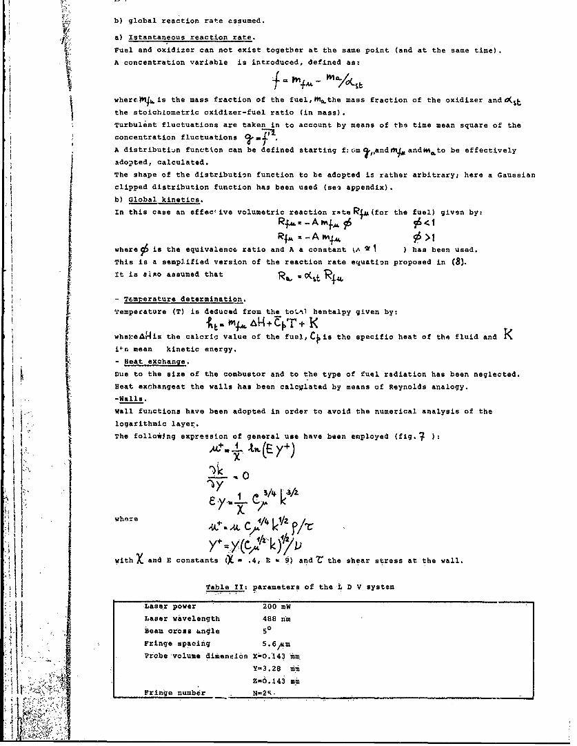
b) global reaction rate assumed.

a) Istantaneous reaction rate.

Fuel and oxidizer can not exist together at the same point (and at the same time).

A concentration variable is introduced, defined as:

where.Mjhis the mass fraction of the fuel,m*the mass fraction of the oxidizer and0('

the stoichLometric oxidizer-fuel ratio (in mass).

Turbulent fluctuations are taken in to account by means of the time mean square of the

concentration fluctuations

A distributijn function can be defined starting f:om .,and '"4Aandlto be effectivelyadopted, calculated.

The shape of the distribution function to be adopted is rather arbitrary; here a Gaussian

clipped distribution function has been used (se3 appendix).

b) Global kinetics.

In this case an effeclive volumetric reaction rate Riu(for the fuel) given by:

where9 is the equivalence ratio and A a constant (A ) has been used.

This is a semplified version of the reaction rate equation proposed in (8).It is aixo assumed that R 4

- T6mperature determination.

Ikemperature (T) is deduced from the tot,1 hentalpy given by:

whe:eAlkis the caloric value of the fuel,Cjis the specific heat of the fluid and

i-n mean kinetic energy.

- Heat exchange.

Due to the size of the combustor and to the type of euel radiation has been neglected.

Heat exohangeat the walls has been calcglated by means of Reynolds analogy.

-Walls.

Wall functions have been adopted in order to avoid the numerical analysis of the

logarithmic layer.

The follo*Jng expression of general use have been employed (fig. ) :

withX and E constants C .4, E 0 9) andr the shear stress at the wall.

Table II: parameters of the'L D V system

-Laser power 200 mW.11 Laser wavelength 488 fm

Beam cross ungle 50

Fringe spacing 5.6,m

Probe -volume dimeneion X&O.143 mmI, , Y-3.28 ii

Z-6.143 mmFringe number N-2r-

19-5

4) RESULTS.

Measurements have been carried out in correspondence of sec. 1, 2, 4 . of fig.Lf; three

conditions I, II, III have been tested during experiments.

Mean values of temperature, axial velocity and swirl velocity were measured.

- Temperature.

Measured and computed temperature di.trAbution are reported in figg. 8 42 2..

In correspondence of sec.2 13,4 the accord between measured and calculated results can

be considered enough good.

Near the injection 1-eud (se-. I e-:perimental and computed results are rather different,

also if, in some cases, a sort of common trend can be recognized at least for model b

in testsl and II, and for model a in test III.

As a general behaviour computed temperature are higher than the calculated ones.

It can be considered that in the injection region (near sec. I ) model b works a little

oetter than model a.

This seams to mean that istantaneous reaction rate hypothesis is not particulary suitable

to be employed in this zone probably bedause of the rather high mixing rate, leading

to a competition between chemical kinetics knd fluidodynamics.

on the other hand also the global kinetics here used does not seem to be satisfactory

in this zone.

It could be deduced that in this region the " LG" kinetics plays an important role also

from the point of view of mean values calculations

Probably near the injecticn heat a global kinetics can hardly be fitted to represent the

real kinetics.

jDown stream the injection znne the introduced models appear to be substantially morJrelyable.

- Axial velocity(i923 2.).

As in the case of temperature, the &argest discrepancies between measured and calculated

results are in correspondence of injection region.

In particul!r the width of the recirculation zone is under extimate in both models.

Down stream the injection they seem to work rather well with reapect to axial velocity.

In tests I and II the global kinetics mo-del appears to offer a better performance near

sec.A ; at the same section both model can be considered practically equivalent intest III.

- Swirl velocity (fig.'3033).

The tred is the same as in the case of axial velocityi the injection region is the most

critical in the comparison.

On the whole, the accord between experiments and theoretical values can be consideredas satigfactory en6ugl .

I! 5) CONCLUSIONS.

What precedes shows that in general the agreement between theory and experiments can he

considered as acceptable, also if near the injaction regioi the discrepancies are not

neglegible.

If however from an engineering point of view the results could be satisfactory, they do

not appear to be adequate, if a more sophysticated analysis of the phenomenon must be

j perfprmed.

In particular near sec. 1 (injection regioni the differencies between measured and

I I computed temperatures are large enough to in~fluence considerably the reaction rate, if

it is made dependent on temperature.

j Then if elementary reactions must be introduced, rather large errors ca arise; f. e. a

pollutants generation analysis can hardy be carried out.

The performancies of both models are rather similar, expecially down stream the injection

rb.gioft.

Also if the global kinetics model seems to lead to better results near the injection

head, it is not able to improve substantially the results with respect to the istantaneous

-:eaction rate hypcthesis.

Probably the rather strong mixing, also increased by the peripheral swirl, is responsible

for thiu kind of behaviour.

It seems that in this zone the introduction of a more sophisticated and realistic kinetic

model is a fundamental stage to improve the agreement between theory and experiments.

Concerning turbulence models, a k -S formulation has been here employed; this model is

at the same time rather well experienced and not particulary trouble some to be used.

It has not been analyzed here if other and more complex models could be more suitable,

also if the peripherical centrifugal field (due to diluition air swirl) can increase the

complexity of the turbulent field and require a more sophisticated analysis.

Thermal exchange has been treated in a rather simple way; on the other hand the rate or

the heat exchange trough the walls is less than 10% of the rate of heat generation !n the

furnace and then not able to introduce substantial changes in the results.

classical time averaging has been adopted here, and other typyG of averaging (f. e.eavre

averaging) have not been tested, also if they are able to give good results in many cases.

From a numerical point of view, the greatest difficulties have been encounteredwith the

equations h&ving rather complicated source terms (k-,Ec equations).

They have been overcomed by means of under relaxation and of a some kind of linearization.

The cou,puter time for the calculation was about 5 minuts with an Univac100/8Ocomputer

with a :,vn uniform 21x21 grid.

6) REFERENCES

(1) Gosman A.D. et al."Heat and mass transfer in recirculating flows",Academic Prz.ss,1969

(2) 1annekes M. and Lumley J.L,,"A first course in turbulence", M.I.T. Press, 1972.

(3) Launder B.E. and spolding D.B.,"Mathematical modlas of turbulence",Academic Press,

1972.

(4) Launder B.E. and Spolding D.B.,in:"Computer methods iL Applied Mechanics and Engi-

neering", vol.3,pp.269-2S9,1974.

(5) Hinze J.O.,"Turbulence", Mc Graw Hill Book C., New York, 1975.

(6) Lockwood F.C. and Naguib A.S.,"Combustion and Flame", 24,p.109, 1975.

(7) Bracco F.V. ed.:Sp~cial issue on turbulent reactive flows", Combuszion Science and

Technology, vo-.13,n.1-6, 1976.

(8) Magnussen B.F. and Hjertager B.B.,16th Symposium (International) on Combustionp.719

(1976).

(9) Durst V., Melling A. and Whitelaw J.H.,"Principlea and Practice of laser Doppler ane-

mometry", Academic Press, 1976.

by laser Doppler Anemometry",AGARD Conference Meeting on: "Applications of non-intru-

sive instrumentation in fluid flow research".Saint-Louis, France, 1976.

(Il)Durrani T.S. and Greated C.A.,"Laser Systems in Flow Measurement",Plenum Press,1977.

g (12)Coghe A. and Ghezzi U.,"Turbulence characteristics in the recirculation region behind

a disc; isothermal and non isothermal flow." 19th Israel Annual Conference on Aviati-

on and Astronautics, Haia, 1977.

(13)Gibson N.M., Jones W.P., Mc Guirk J.J. and Whitelaw J.H.,"Fundamentals of turbulence

and their application in calculation methods", Imperial College, London, 1978.

(14)Coghe A. and Ghezzi U.,"LDA Signal Analysis", Dynamic Flow Conference 1978, Marseille

lFrance), 1978.

-OBSERVATION

In-many cases the results of test II are very similar to results of test I, and are

not reported here.

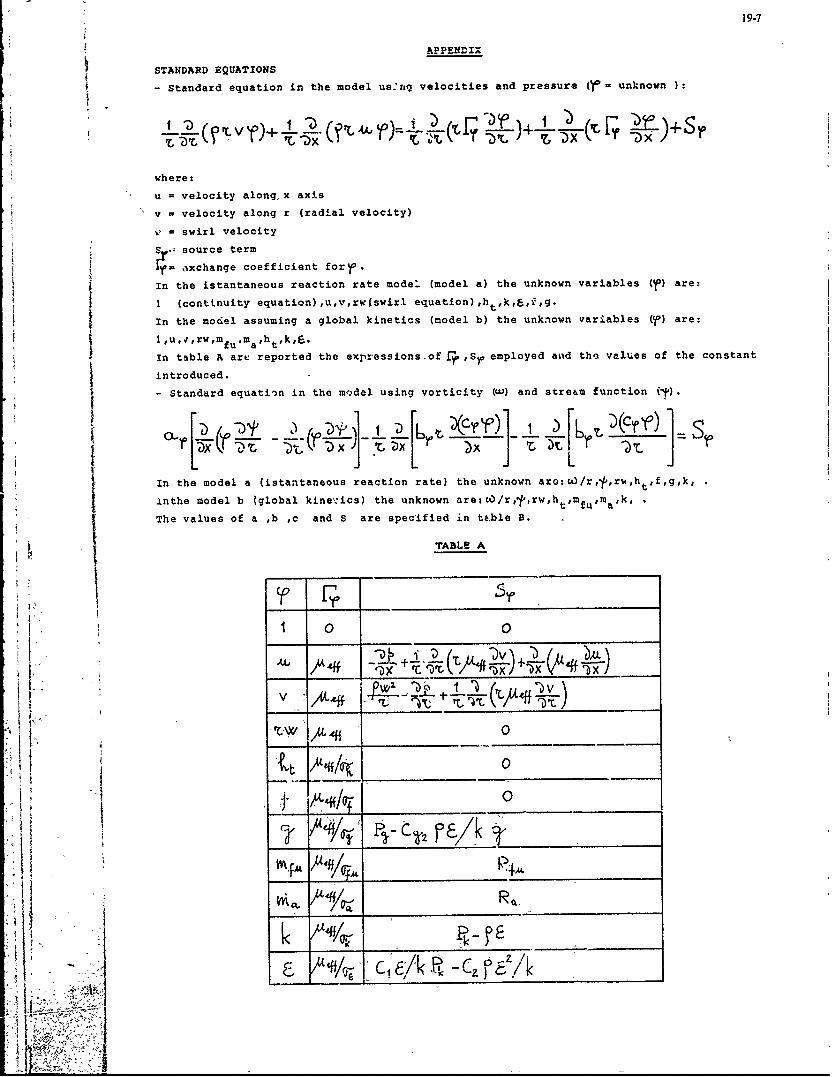
19-7

APPENDIX

STANDARD EQUATIONS

- Standard equation in the model us:nq velocities and pressure (r= unknown ):

where:

u = velocity along, x axis

v - velocity along r (radial velocity)

= swirl velocity

S -, source term

=xchange coefficient fory'.

In the istantaneous reaction rate model (model a) the unknown variables are:

I (continuity equation),u,v,rw(swirl equation),ht,k,6,f.g.

In the model assuming a global kinetics (model b) the unknown variables (f) are:

1 ,u,,rw,mfumathtek,S.

In table A arc reported the expressions-of r ,Se employed antd the values of the constant

introduced.

- Standard equatin in the model using vorticity (W) and stream function (-t).

In the model a (istantaneous reaction rate) the unknown aro:")/r,,1 r%,ht,fpgpk,

inthe model b 1global kine\ics) the unknown are:LO/r,1t,rw,ht,mfu,m,k,

The values of a ,b c and S are specified in table B.

TABLE A

, .5r

V ff ox_ _ _ _ _ _ _ _ _ _

* Ki1 0:/g 0o,.. 1Woq 0

~bAft/C t___

__~l - C~Pk

Ii ___

U ~~ ~ ~ ~ E r*.~ _________

TABLE B

I •~

0 ~ 0

,U6- v z VC r''1/r 4!'1

!.!t

+ Ga/fta clippe ditiuin cin

nu'fI' I

Q- 1. C1, 1-++.9?Q0 tC

The Gaussian clipped p.d~f. has the shape shown in FIGoaj it can be quantitatively

define4 f.e. by means of the method reported in starting from the calculatedi ~ ~values of f and g". (

; . o- : o -;FIG. ak,

DILUION I

1 . Dilution air line- -

2. Primary air line4. Valve FUEL PRIMARY AIR

6. Pressure gauge6 6 6 7. Flovneter

4- 41PRIMARYAIR

FIG.

FIG. i

I GLASS WINDOWS

IJCIION.I4EAD COMBUSTION

FIG, 3

SEC 1 2 3 4

A# Z W S

1 -E T.VELPORTR MEASUREMENTS

FIG. 4

L.2LASER a. 9.5.2 .P

J..S. -Beam splitter and fequency shifterE FF.. Frequeficy-generator fcr the Bragg Cell E

C.C. -Cordbustion chamberP.M Photovltiplier

P.S. - Power s upply F-PiiP.A. - PreamplifierP.B.F. - pass-bind filterC.P. -Counter ProcessorT. Thermocouple

FIG. 5

T

wall

AXIAL TEMPERATURE

TEST IU - EXP.

-200 - - -MODEL a

-- -MODEL b

.2 .

FI. 6 FIG.'7 Fr,8

T

600

- -- Model a -.- Model bj

.02 .06 r .

FIG.

1200

RADIAL TEMPERATURETEST I - SEC. 2

-EX0.

400. . . MODEL a

--- 40DEL b

.06

FIGit fl.

1200

800

.--- MODEL b-

A.02 .06 A

FIG. ii (n

J-1

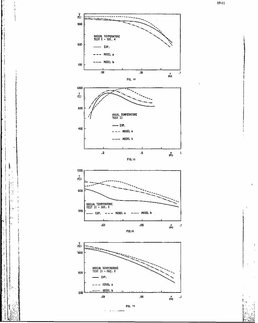
19-11

T----------------------- --- -- -- -- -- -- -- -- -- -- -- -

900..

RADIAL TEIMPERATUIRE

TEST I - SEC. 4N

-EXP.

--- MODEL a

MODEL b100-

FIG. 12

804.

400 - EXP.

MODEL b

.2 .6 x I)

FIG. 13

1000

VC)

600

RADIAL TEM1PERATURE

20 - EXP. IIODEL a M..-lODE b

.02 .06 .1

CC))

600 TEST ?I -SEC..2'

MODEL a

-... KDELb

-3.02 .06 .1

U ~FIG. 1

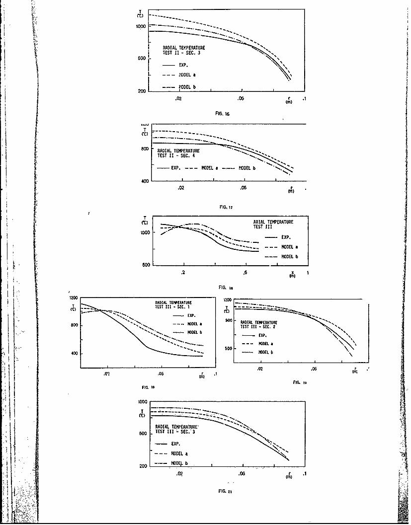
1000

RADIAL TEM.PERATURE

[0- EXP.

L = flEL a

MO.-~!DEL bj

.02 .6r .

FIG. 16

80 RADIAL TEMPERATURE*TEST 11 -SEC. 4 -.

EXP. MODEL a M.- ODEL b

400AIL

.02 .06 j£ FIG. iij

Ct) - -- .~ .AXIAL TEMPERATURE

1000 ---. .* TET III

-0 .2 - MODELaK---.-MODEL b

.2 .6

RADIA T~lIERATFEIG.

1200 1200

800 . -- MOEL 900RADIAL TEMPERATURE-TTEST III - SEC. . %

RADIA TEDIA TRATURER$00 TEST III SEC.

EEXP.

--- MMOELL

ii40 20 -.-. DN0E

.02 .06

~ FIG.IG.

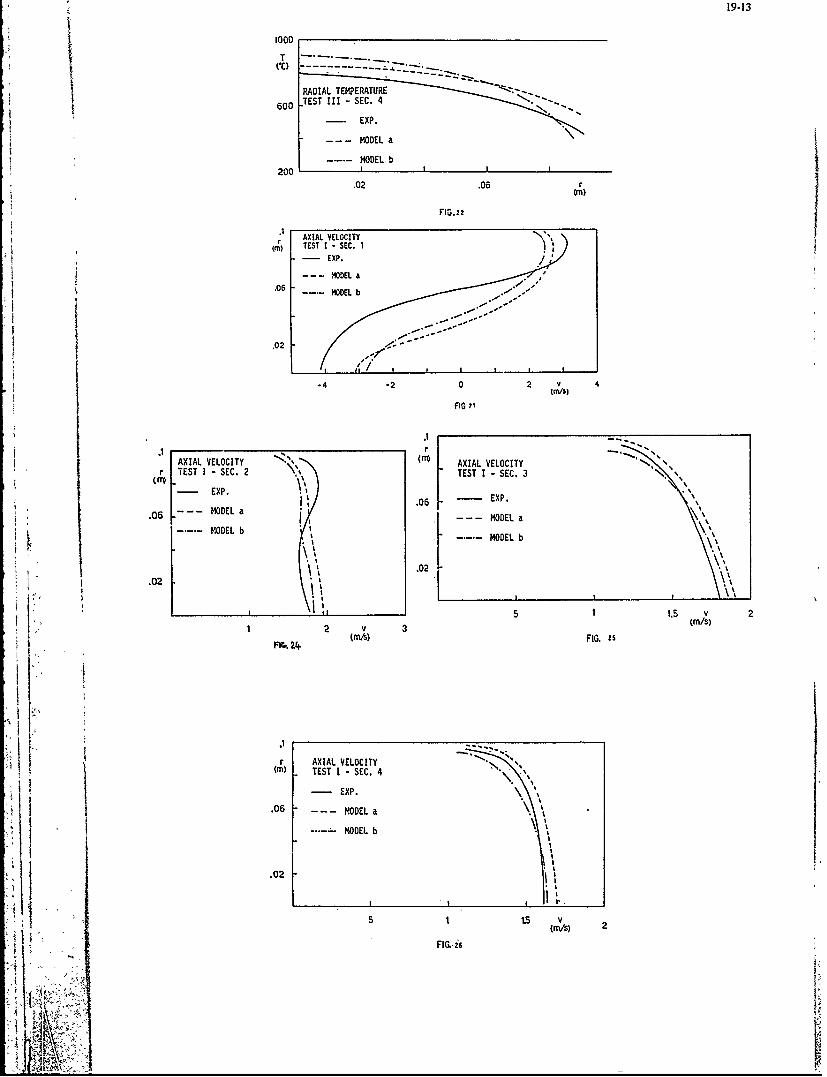
19-13

60TEST III - SEC. 4

- t-- ODE a

.02 .06 rm

AXIAL VELOCITY N'

TETI-.SEC.1

MIODELab

.02

-4 .2 0 2 (rn/S

FIG,?I

AXIAL VELOCITY N\AXIAL VELOCITY- -

rITEST I -SEC. 2 [ TEST I -SEC. 3

MOEL a .061 - EXP.

5

.06 MODEL aMOEa

MO E. - - --- M ODEL b

.02 5 1.5 V 2

7 1 2 v 3FI.2

AXIAL VELOCITY

ml TEST I -SEC. 4

to Exp.a

MODELb

.02

5 Is

FIG.i. m/sI 2

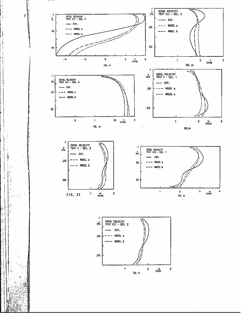
1 AXIAL VELOCITY

TETI-E.1L)TEST III -SEC. 2

06 -.- MODEL b5102 02

4 -2s2 4 2 V 3Fr,. Fai

___________________________________________SWIRL VELOCITY

AXIAL VELOCITY 5~ TETI-SC 1TEST III - SEC. 4 - EP

06- - MODEL .0a OE

Ii'. .02

FC% (rnvs)F, fM30

SWIRL) SVIRLVELCTT

r TST -SE . 2 '\r TEST III - SEC. 1EXP- NE. .

EXP.0 6 MOD0EL a I0Ea

-.-.- ~0 MODEL .. D~

.02 0

1 w w 4

FIG. 31 1 ms 2I )z(A

~. SWIRL VELOCITY .(on) TEST III - SEC. 2 *

EXP.

.06 MiODEL a

MODEL b I

.02 I

2 w 3ItvsFG. 33

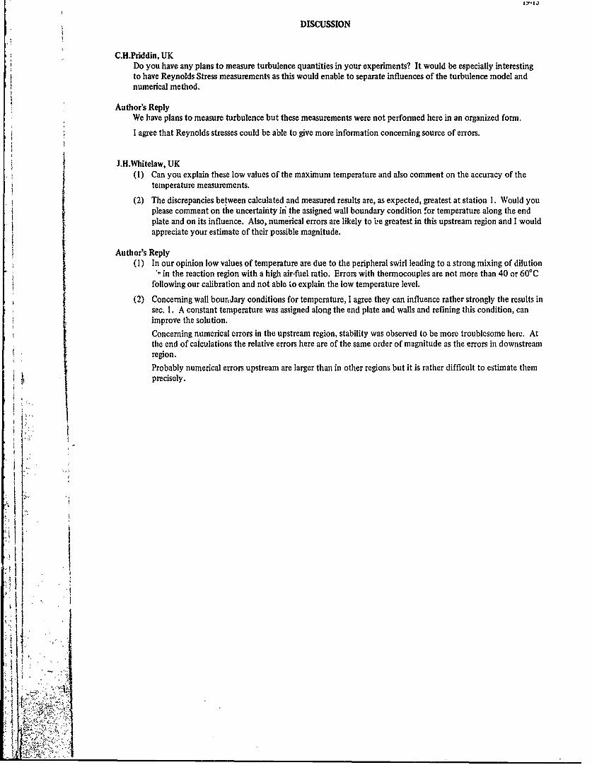
DISCUSSION

C.H.Priddin, UKDo you have any plans to measure turbulence quantities in your experiments? It would be especially interestingto have Reynolds Stress measurements as this would enable to separate influences of the turbulence model andnumerical method.

Author's ReplyWe have plans to measure turbulence but these measurements were not performed here in an organized form.

I agree that Reynolds stresses could be able to give more information concerning source of errors.

J.H.Whitelaw, UK(1) Can you explain these low values of the maximum temperature and also comment on the accuracy of the

temperature measurements.

(2) The discrepancies between calculated and measured results are, as expected, greatest at station 1. Would youplease comment on the uncertainty iii the assigned wall boundary condition for temperature along the endplate and on its influence. Also, nume'ial errors are likely to be greatest in this upstream region and I wouldappreciate your estimate of their possible magnitude.

Author's Reply(1) In our opinion low values of temperature are due to the peripheral swirl leading to a strong mixing of dilution

" in the reaction region with a high air-fuel ratio. Errors with thermocouples are not more than 40 or 600 Cfollowing our calibration and not able to explain the low temperature level.

(2) Concerning wall boundary conditions for temperature, I agree they can influence rather strongly the results insec. 1. A constant temperature was assigned along the end plate and walls and refining this condition, canimprove the solution.

Concerning numerical errors in the upstream region, stability was observed to be more troublesome here. Atthe end of calculations the relative errors here are of the same order of magnitude as the errors in downstreamregion.Probably numerical errors upstream are larger than in other regions but it is rather difficult to estimate themprecisely.

I I

t

o~

4

20-1

MODELISATION DES FOURS ALItIENTES A L AIR ENRICH! EN OXYGENE

R. GUENOT, A. IVERNELL'AIR LIQL'IDE C.R.C.D.JOUY-EN-JOSAS, France

F.C. LOCKWOOD, A.P. SALOOJAIMPERIAL COLLEGE OF SCIENCE AND TECHNOLOGYLONDON SW7, England

La modelisation num~rique des chambres de combustion utilisant des brileurs aliment~sa l'air fortement enrichi en oxyg~ne, pr~sente des difficultds particuli~res li~esd'une part aux dissociations thermiques se produisant A haute temp~rature, et dCautrepart au r6le accru des 6changes par rayonnement.

Le prdsent article montre comment on peut adapter les programmes de calculs existant,afin de tenir compte de ces ph~nom~nes.

Le mod~le utilis6 est en cours de vdrification au moyen de mesures effectu~es sur unfour exp~rimental de 300 kW, conqu pour fonctionner avec des brOleurs a haute intensit§aliment~s par du gaz naturel et de l'air fortement suroxyg~n6, ou m~me de l'oxyg~ne pur.

Les premiers r~sultats expdrimentaux sont en hon accord avec les prevsions du mod~le.

1. /INTRODUCTION/1.1. OBJET DE L'ETUDE

Pour certaines applicatbns, l'ndustrie utilise d(- plus en plus fr~quemment des br~leurs aliment~s'en air suroxyg~n6 ou m~me en oxyg~ne pur, impliquant une dissociation appreciable des produits decombustion.

Les programmes de simulation des chambres de combustion qui ont 6t employ~s avec succ~s (1)(2)pour los brOleurs classiquos, ne donnont pas satisfattion pour los brOleurs A air fortement enrichi enoxyg~ne.

Le prdsent article expose los premiers r~sultats o'une 6tude destin6 A 6tendre ces programmes aucas d'un comburant, dont la richesse en oxyg~ne peut atteindre 100 %

Dans los flammes a haute temperature resultant de la suroxygdnation du comburant, los dissociationsthermiques des produits de combustion jouent un r6lo capital. Elles absorbent en effet une partie importantede la chaleur normalemont ddgagde par la combustion, et diminuent ainsi la temperature des flammes.

Cette chaleur, stock~e sous forme chimique, ost d'ailleurs r~cupdrable par recombinaison au niveaudes surfaces do pieces ou des parois de fours, de sorte que c'est finalement l'enthalpie, et non la tempera-

ture, qui intervient dans les 6quations de transfert thermique par convection et diffusion.

Par contro, si V'on veut incurpurer dans le mod~ie les echangos par rayonnement, il est n~cessaire,Ien cours do calcul, de tenir compto do la tempdrature et - a uii d~gr6 moindre - des fractions massiques desesp~ces ex-';tant A l'dquil-ibr6.

uans la pr~sente communication seront expos~s successivement :los modales math~matiques r~cents,utilis~s a l'Imperial College, pour la simulation des chambres de co mbustion, les mnodifications apport~espour tenir co~npte des dissociations, los m~thodes exp~rimentales mises en oouvre et les premiers essiisdo confrontation entre'les rdsultats de calculs et les r~sultats exp~rimentaux.

1.2. POSITION DU PROBLEME

4 La preuve ost maintenant faite (voir par exemple (1) et (2) que lo forictlonnoment des chambresde combustion aiiment~es au gaz et A Pair peut 6tre pr~vu avec tin d~gr6 d'exactitude largemont acceptabledu point de vue des applications, du moins pour les brOleurs n'utilisant pasou pou 1'offet do "swirl".Quoi qu 'ii e n soi t,, Ile probl me trai t6 dans Ile pr'esent, arti cl e a 60 jusqqi 'ci peu dtudi 6. 11 concerne 1laprevisi n des chambres d6 combustion ali'ment~es :tu gazet A l'air enritili on oxyg~re, ou m~me a I 'oxyg~nepur. Cos rechorches impliquont des prohlffies cbmpldmentdires do modelisation plut6t d'ordro chimiquequ'hydrodynamique.

Etant donn6 qu'oi. peut, supposeravoc r~alisme que, 6Wir la pl'upart des fours, le taux de r~aciionglobale est gouvern6 par le taux de Gi ssipati6n do la turbuliince~ot non par la cin~tique chiniique, on peutconclure que la seule forme do chimie n~cessaire 'dans le ca .degflanm s 'a haute temp~rature resultantd'unenrichissoment a- l'oxyg~ne es t la chjniie d'6quilibpe,.L1,. ectif ussontiel de 1 V',tude pr~sent~e dans'cet article est~d'incorpo.rer un tpaitemednt de 1'6quilibre ehinnu asn jnin ~cnm edasuprocWd g~ndrl de pr6vision d~crit en (1)., La valour des p,&vosions du-proc~d r~sultafit -font 1 'objetd'un programmie de ve-ri-fica'tion ex'pdrimeintale en cours d'ach~voment,-utilisant des flammies enrichies AV ox4nd, et r~alis au C'entre d& Recherche CLAUDE-DELORIV Z LI'I LIQUIDE.

I x.

Le problfte du "swirl" W'est oas abord6 ici. 11 convieric de rerarquer au passage que le manque devalidation pour les exemples de brOleurs 5 grand nombre de str r1 provient d'autres limitations, a savoir,que les 6coulements avec swirl sont imparfaitement dvalu~s par le mod~le de turbulence "standard" A deuxdquations, car l'hypoth~se inh~rente d'une viscosit6 tur-bulente insotrope nWest pas satisfaisante.

7\ Un mcd~le turbulent de tensions de Reynolds serait pr~f~rable, mais la surcharge due aux estima-tions des param~tres n~cessaires, ajout~e aux calculs d0;A coOteux n~cessaires A la pr~vision des chatibresde combustion, le rend !oratiquem'ent i nabordable. Pour-contourner cette difficult6, ii suffit d'emplolyer unmod~le algdbrique 6&onomique pour les tensions de Reynolds de la for-me d~crite en (3), mais il r-este encorea dtudier son application aux chambres de combustion. Le br~leur utilis6 par L'AIR LIQUIDE ne comportantpas de swirl permet de faire des 6tudes de validation a l'aide de solides connaissances de base obtenuesdans la modelisation des flarnmes sans swirl et non enrichi 2s a l'oxyg~ne. En fait, l'enrichissement al'oxyg~ne per-met la stabilisation de la flamme, en l'absence d'une zone de recirculation intense a lasortie du bruleur.

11. / LA MODELISATION PHYSIQUEII.1. LE MODELE DE TURBULENCE

atesOn emplcie le modfle usuel de turbulence j deux dquations dans lequel on r~soud les 6quations re-ltvsA 1'6nergie cin~tique de la turbulence, k, et a son taux de dissipation, &; une viscosit6 isotrope

effective 6tant d~finie A partir de ces deux valeurs (3). Malgrd des recherches poussdes sur des mod~lesplus compliqusdans lesquels on r-~soud des 6quations pour les tensions de Reynolds elles-mimes, (voirpar exemple (4)), rien n'a encore per-mis de d~placer le mod~le k-e dela position prddminente qu'il occupedans les calculs d'application par-ce qu'il repr~sente une combinaison pratique d'6conomie et d'exactitude.

En ce qui concerne les dcoulements sans "swirl" dont on parle ici, les imperfections eventuellesde ce mod~le peuvent 6tre en grande par-tie attribu~es non pas a l'usage du concept de viscosit6 effective,mais aux d~fauts de modelisation des 6quations pour k-e qui ne sont en aucun cas faciles A rectifier.

11.2. LA MODELISJATION DU RAYONNEMENT

Dans le genre de four consid~rd les pertes de ch~leur aux parois r~fractaires ne sont pas tr-~simportantes. 11 nWest donc pas n~cessaire d'avoir recours A un mod~e tr-~s pr~cis de transfert par rayon-nement. Nous avons utilis6 pour le rayonnement le mod~le de flux' d~cr-it en detail en (5), qul assure uneexactitude acceptable pour des d~penses tr~s limit~es. Ce type de m~thode est bri~vement r~sumde dans leparagraphe suivant

La repartition angulaire de l'intensitd est repr-dsent~e par une sdrie tronqu~e de Taylor, substi-tu~e dans 1'6quation du transfertde chaleur par rayonnement. Cette 6quation est ensuite int~grde sur desangles solides bien choisis, le nombre d'angles correspondant au nombre de termes dans le d~veloppement.On obtient ainsi un syst~me ferm6 de six equations aux d~rivtes partielles du premier v)-dre ayant pourinconnues les coefficients du d~veloppement de Taylor. Pour le probl~me A deux dimensions trait6 ici, nous

* ne retiendrons que quatre termes de la s~rie. Afin de rendre possible leur solution A l'aide de l'algorifimenum~r-ique a matrice tri-diagonale employd pour les calculs d'fcoulement, les quatre 6quations du prerwieror-dre pour les coefficients sont combin~es de fagon A donner la paire des dquations du second or-dre ci-dessous ' ~ ~ ~

-F -z k 3 r - S E

oG r et z sont les coordonn~es radiale et axiale, k est le coefficient d'absor-ption, E =O'T est la puis-sance dmissive du corps noir, et Rr et Rz sont relies aux coefficients de la s~r-ie de Taylor. Ces 6quationsne sont pas appliqu~es directement au gaz de combustion mais a un syst~me classique de 4 gaz gris dquivalents.

11.3. MODELISATION DEj PROCESSUSItHERMIQIELa prevision correcte des processus thermique est tr~s importante pour le d~roulement des calculs.

Le mod~le utilis6 est d~crit en'detail dans (6),

En ce qui concerne les transports de chaleur et de masse accompagnant la combustion, on fait M'y-I ~ 1 oth~se classique que tous les coefficients de diffusion turbulente sont 6gaux. Le melange des constituantsest alors rdgi par une 6quation portant sur le rapport de melange f quantit6 inddpendante de I '6volutiondes reactions et 6§ale A la fraction massique de combustible dans 1 '6tat imbraM~

Similairement le transport de chaleur est caract~ris6 par une seule equation enthalpique oa latemperature et la composition chimiqe n'interviennent pas explicitement.

En ce qul concerne le processus de combustion, on suppose en premier lbu une rdaction chimique glo-bale simplifide entre U~ combustible gazeux et le comburant aboutissart a la production de C02 et H20.Esecond lieu, on surajoute A ce schema de base les calculs d'djuilibre chimique expos6 dans la sectionsuivante, pour tenircomptede la dissociation des produits de combustion.

Pans- le schema de base 1'6tat theririuu'ynamique du rhelange r~agissant est fonction de deux variablesseulement ; la fraction de melange, f, et -le deord d"avanc~pient, r, d~fini par r =(mj. - mu/mb - mj,u)(reactedness), ou mu e'st la fraction massique'di toute esp~ce~ciiimique rdagissante, et oumg'etu/md~signeht le fluide brMl et ncn-br0l. Pour une fl0anMe de diffusion, r = 1, et la turo'ulence entraine desfluctuations de f-Uniquement, tandis que pour une flaniie parfaitemdnt pr~m~langde, f est constante et rvarie.

On suppose pour las fluctuations des deux variables, que les fonctions densit6 de probabilit6 (d.p.)ont des formes a priori. Pour le tas de f, on utilise une distribution Gaussienne "sectionn&e", compl~te-ment sp~cifi~e par la connaissance de la fraction de ni~lange moyenne dans le temps, f. et sa variance,

g F-f12.L'hypoth~se d'une cinthiqua chimique rapide compar~e au taux de melange .urbulent paraitbien fond@ dans la plupart des calculs d'applications; elle est compatible avec une loi de probabilit6(d.p.) simple de r constitu~es de deux fonctions delta (au sens de DIRAC), ces fonctions de delta 6tantcentr~es sur les valeurs limites r =0 et r = 1. La grandeur des fonctions delta est eun liaison directeavec le degr6 d'avancemant moyan dans le temps, r, qui peut @tre obtenue a partir de la solution d'unedquation de bilan portant sur la fraction molaire moyenne (dans le temps) de l'une des esp~ces rdagissante,le combustible par exemple.

Une formule est n~cessaire pour le taux de reaction moyen de l'espkce choisie, qui repr~sente unterme de source dans l'dquation de bilan consid~r~e. Dans 1Phypoth~se 00 la reaction globale est contr~lepar le taux de c~iange de turbulence, le taux de reaction est 6gal au taux de dissipation des fluctuations4de r. On a proposd plusieurs expressions reliant le taux de dissipation de la turbulence 5 des variablesconnues. Ils ant une base physique commune, bien que voisine. Heureusement, les calculs sont insensibles5 la forme exacte de l'expression. Celle que nous avons utilis~e est

R =CP (nui b flhj u ) [rF 1_ r] 112 elk

ouj est le taux de reaction mayan dans le temps de 1'esp~ce r~agissante choisie. Dans cette formuleincrit lhypoth~se simple, que le taux de dissipation des fluctuations du degr6 d'avancement est pro-I

portionnal d'una part a leur 6cart-type, qui, pour la loi de probabilit6 simple constitu~e de deuxfonctions de deltas,

s'6crit : r (1 - 12;et d' autre part a 1'6chelle de temps de grands tourbillons, '-/k. La constanteempirique, C, a W triuv~e 6gale a 0.35 environ.

On s'int~resse dans la plupart des cas aux quantit~s mayennes dans le temps et cette moyenne dansle temps s'exprime pour toute propri~td thermodynamique, 0 , par

IACW =jJ (f,r) p(f,r) dfdr

aD p (f, r) est la fonction jointe de probabilit6 de dersitd pour f et r. 11 y a peu de chances que lasvariations de f et r soient fortemant correldes; on peut doric, de mani~re justifiable, d~composer p (f,r)en s~parant les variables et 6crire

J ,~ 0(f, r) p(f) p(r) dfdr

o0_p (f) et p (r) sont respectivemant les d.p. Gaussjc-nna sectionn~e, et delta coupl~e, mentionn~es

ci-dessus. Pour plus de details on se rdfereaA()111. / PRINCIPE DE LA METHODE NUMERIU DREOUTION

111.1. EQUATIONS A RESOUDRE

On doit r~soudra des 6quations pour les composantes axiale, u et radiala, v, 1'6nergie cin~tiquede laturbulence, k, et son taux de dissipation , 9 , la fraction de m~lanqa, f, at sa variance, g, lafraction massique du combustible, mfu, l'anthalpie sp~cifique, h, et anfin las param~tres de rayonnementRr at Rz. Pour la g~omdtrie cylindrique polaire trait~e ici, ces dquations soot toutas de la farina

(ryuo) + :-r (rv)r r. rr Oro

ou 0 repr~sente toute variable ddpendante &ionc~e ci-dessus, et S, est un terme de source (par examplePfu dans le cas de l'dquation relative a mffu, fraction massique r~siduelle de combustible).

111.2. METHODE DE RESOLUTION

Les 6quations soot r~solues A laida dUi processus standard de diff~rence finie d~crit en (8) et(9,et raltachM au coda d'ordinateur TLACH-T. Les ~grillas d'ordinataur utilistas comprennent 40C olveojds

qul, lorsqu'.ils sont aispos~s convenablement, donoent des r~sultats ind~pendants de la grille.

Les conditions-aux limites -utilis~es correspondent A celle dv brOleur expdrimental. Certaines

La ~atrsiusdasrto td&iso ugzso alsd nd1 lsiu a rsdonn~es manquantes sont remplace's par des estimations raisonnablas (6missjvit de la parai. par example).Ichdque iteration las variables corraspondant aux dquations ci-dessus sont-an principa t6values, ainsique les gr~idaurs quli en ddpendent.

HToutefois ler'ajustement des vala urs moyanneE li~es au modfle stochastique de combustionWintervient que tous las 5 A 10 iterationis.

IV. PRIS EWCMPTEDES 7'ISSOCIATIONS INTERVENANT A HAUTE TEM-PERATURE/

IV.-. RINIP DUREAUSTM T A MOENDES-CALCULSD'EQUILIBRE

Nous consid~rons qu'an chaque point, 116tat tharmodynamique du mflange est attaint en 2 @tapesa cin~tique tr~s rapide.

La oremi~re est une combustion fi~tive dans laquelle le melange de depart COMBUSTIBLE + OXYGENE(+ INERTE) donne CO2 + H20 + EXCES (+ INERTE).

Par EXCES on entend soit'l'exc~s d'oxygene, soit l'exc~s du combustible subsistant apres combustionstochi -om~trique. Le melange de depart est par d~firition le me~lange local qu'on obtiendrait en labsence de

j combtisti on.

Dans le cas general oD i1 peut exister plusieurs arriv&es de comburant (oxyg~ne pur et air Dlus oumomns enrichi par exemple), et oD le combustible peut contenir des inertes, la composition de depart estd~finie par les fractions massiques f et i de combustible et d'inerte respectivement. Elle s'obtien.t par2 equations de transport ne comoortant pas de terme de source. Dans le cas lirnite d'un pr~m~lange completf et i sont constants. En l'absence d:6change par rayonnement l'enthalpie du melange reel hAp est fonctionlin~aire de f et i dt he n~cessite pas d'eqUation particuli~re.

Par contre, si le rayonnement est pris en compte, l'dquation. de transport de l'enthalpie comporteun terme de source, et doit 8tre r~solu s~par~ment. Il conduit A une valeur locale de h diff~rente de hADet l'dcart traduit l'influence des pertes par rayonnement. On peut le caract~riser par un rapport d'adia-baticit6 sans dimension Pdffini par

'P ..L..R oQ h est une enthalpie de reference prise 6oale a cellehAD- hR R

du melange W16l ideal (non dis-oci6) rameri6 a la temperature ambiante.

La seconde 6tape est un retour adiabatique aux conditions d'6qiuilibre chimiques, que V'on peutobtenir par un sous-prograine d'6quilibre chimique, dans lequel les variables d'entrdes sont l'enthalpielocale h et la composition 616mentaire dA.iuite de f et i.

En fait, 11 cs4 pus commode d'utiliser au lieu de h le rapport d'adiabaticite Y d~fini plus haut.

L'utilisation syst~matique d'un sous-programie d'6quilibre pour calculer en chaque point et Achaque iteration la temperature, la densit6 et la composition en fonction de f, i et est exclue du pointde vue 6conomique.

La difficult6 a W tourn~e en calculant au pr~alable des valeurs d'6quilibre pour un nombrelimit6 de valeurs de5F , f et i, et en interpolant au moyen de formules d'ajustement.

f Dans une premi~redtude Jimit~e au cas extreme d'un brOleur a I 'oxyg~ne pur, un tableau A 2 entrees*f, f comportant eriviron 100 rdsuitats d'6quilibres a W 6tabli A partir de sous-progravnes d'dquilibres

j drives de ceux de HARKER et SMITH(1.

Commie premiee approche, ces r~sultats ont W condenses en une formule d'ajustement du type

TEQ A + A 1 f =A2 f2 +A3 f

avec les Ai sont fonctions de 0 et une forrnule similaire pour la densitd.

Si on n~gligeait a ce stade les fluctuations de la fraction de melange, on pourrait utiliserdirectement cette formule pour chaque point, en utilisant pour f la valeur donn~e par 1 'quation de trans-

port correspondanteTEQ A 0 + A1 f + A2 (f)

2 + A3 (f) 3

En r~alitd la tormule d'ajustement fournit une valeur instantanke a partir de laquelle la valeur moyennecorrecte s'exprime par:

TCORR- = Ao+ f +A2 (f )A 3 (f ) soit encore

g d~sirant comme pr~c et la vaiace de fluctuatonde fet M3un moment non-centr6 du 30ordre

M3use telcle foruleet en paricipes rtre dan la zons esfuctin de frbbii- cosontr prtadent.

Une autre m~thode, en cours de r~alisation, revient a utiliser un ajjustement par trongons At~alculer directement 1 integrale

~ ITCR JT Q (f) -p ()d f

par integration num~rique.

IV.2. METHODE ITERATIVE DE CORRECTION DU RAYONNFMENTI:: La m~thode de r~ajustement expos~e ci-dessus suppose connue l'enthalpie du melange en tout point.En r~alit6 l'dquation enthalpique contieint un terme de source qul ne pout 6tre calcu1M correctement par lerod~le de rayonnoment d~crit prkc~dermint, que Si la ternp~rature et )a concmntration des espkces absor-tbantes sont-eux mdme connus. 11 convient donc d'effectuer les r~ajustement n~cessaires au cours iraions successives. Au stade actuol nous nous sonmmes born~s A des r~ajustertents de temp~rature et de densi-

t6.

V.,/ DISPOSITIF EXPERIMENTAL7

L'installation comprend essentiellement une chambre de combustion et des moyens de mesures destemperatures, et de vitesses. de pr~lvement de gaz et de aonmt

V.1. LA CHAMBRE

Cette chambre est un four oxp6-imental (figure 1) revdtu intdrieurement de rWractaires en corin-don (94% d'alumine), et permettant c'atteindre des temp~ratures de 2000 X.

Sa capacit6 de chauffage nominalo est de l'ordre de 250 kW mais pout varier pratiquoment entre150 et 400 kW en fonction du taux d'oxygdnation du comburant et des temp~ratures intrieures du four aux-quelles on veut faire los essais. 11 est dquipd pour fonctionner avoc des combust4bles Hiquides et gazeux,et coniie comburant de 1 air suroxygen6 et do 1 okyg~ne pur.

Ce four est muni d'un certain nombre d'ouvertures lat~rales qui permettent l'introduction dessondes de mesure (temperatures, vitosses) des prises de gaz, et des radiom~tres.

Des thermocouples incorpor~s dans la parol interne permetten't de suivre les tempdratures int~rieuresen 3 points du four sur une mdme g~n~ratrice.

V.2. LES BRULEURS

Los brOleurs utlis~s sont du type industriel ")face mange", pour 6viter tout risque de rentr~ede flamme (figure 2).

Ils comprennent

-une arriv~e do gaz combustible (methane) pat- une canno axiale, d~bouchant par 6 trous f,,;sant unangle do divergence do 200 avec -.~ e dispositif assure un meilleur melange du gaz avec l'oxyg~ne p~ri-ph~rique.

-une arriv~e p~riph~riqucd'oxyg~ne, dont la section~ ost adapt~e au odilt mis en jcu, de fagon A

conserver tout au long des essais wta vitesse do sortie d'oxyg~ne relativement constante.-une 26me arrivde p~riphitrique d'air dont la section est 6galement ajust~e au debit do ce combu-

rant.

V.3. MESURES DES TEMPERATURES DANS LA FLAMME

Los temp~ratures atteintes dans los flanmes suroxyg~n~es Atant souvent s'up~rieures A 2000 K, il6tait n~cessaire ce disposer d'un pyrom~tre ayant des performances sup~rieun s cellos d'un pyrom~tre a

* aspiration ciassique.

L'appareil utilis6 a W du type a "double col sonique" avec lequel on determine la temnp~rature parvariation do masse volumique apr~s d~tente sonique CL-etidde cot appareil a W r~alis~e par 1'0.N.E.R.A.(11\.

-Principe du double col (figure 3)

A oartlr do 1'6quation do BARRE do ST VENANT A la traversde d'un col sonique et la relation duHUGONIOTI on d~duit le debit A travers un orifice sonique en fonction do la pression et do la teiip~ratured'arrdt. Aux faibles vitesses auxquelles on travaillo, ces valeurs peuvent 6tre confondues avec los valoursstatiquos. La figure (3) indique la m~thode do calcul et, precise los notations utilis~os.

La mesure porte sur los inconnues du second membre (PI P2i T2), On notera quo ' I et M1 sont desfonctions do la temperature cherch~o T1, ce qul n~cessite un caicul par iteration.

Lei 'u rapport des sections des cols a W d~termin6 par talonnage avec un pyrom~tre A aspirationmn 'nthermocouple en platine dans 1uno zone do temperature allant jusqu'a 2000 K.

V.4. MESURE DES VITESSES

La mesure des vixesses ost faite do fagon classique avoc une "Sonde do Prandtl" refroidie par eau.

<1Los deux prises do prossion sont reli~es A vun capteur diff~rentiel ACB tr~s sensible dort le signalMlectrique est enregistr6 sur un Servotraco.

V.5. ANALYSE DES GAZ

Pour chaque flaime et a chaque fen~tre des prdldvements do gaz ont W effectu~s au moyen d'une~ Ii;.;-.canne d'aspiration 6nerg~tiquement refroidie. Les gaz supposes "1trenip~s" sont analyses au chromatographe,

qui fournit les cor:.ctntrations molaires en C02, CO, H2, N2 02.

l~Eant done les dicisiametonsimprateLs rnEcontrs a~ins eHs faea hate teupdrsouee

la rapidit6 de recombinaison des esp~ces dissoci~es, il a WS n~cessaire de disposer d'une sonde de pr6-

Suemnt a roge re artib~em ~ged'ouvertr. La emetan is e dPontune tanede ane A teravqesdole ue la msureo des tel u d Vned la scorsndire 1cumn elle n esureompiqte, e ore-foun isi pa 'ppain deridsett apthde det psCMD enfcc monchomale (eul et tdiemenrar crcla to

peret lamesrnnaio de acteuren d'ssivifetu~ toale ye eprmte aonmn oa

- -un pyromftre A fil angle d'overture"(2 trarsq permettn davsedu e rnesuer fle A raneenle fu pre un poir de a temdfpertr ovaiinte "copenembl e or-lammevu r cpie oint. n~e

Lornes pr Psulato de aacul actue deementIdsponibles doivent qte ( EX et~ cm~ae rvires, carI~ ~~pe ls ne tenents ompt dijfces dniersierfectonts q~ lshdt(nert drceApri

del ulld pyorteab "rningelovrtrit7ts~aire) u ere em).e eraonmniq parmn poirnt la pacesi dU ount rouirt e disoiinsel our-fm obtenir e poit. aals

chmr Les rsultats de meu cuteetdsoilsdiet6re cosdrscmepoiorespondnts

La n reierepa campage dessaeries ayat de tremintrropus Apls sut dunet~ration duct fourt

nicessitnt dimprtntela rerat6ionour vos pusotn ou r pbe de rdsultats xpriments.

La iune nou)eleapagsne dsais cest2 actesn le cors d eprtr acu~ x el

Soubeetls rsrvet de onfiratiodes premiers.rsasdsoils amtoepoo~ aatemeLrad predire de faone satisais antle chamres dnecombustionacoupte ten ds richates paor

rayonnement, des flutats ertides, discaions chimei ues apprsn hae tempratu xnrentu

VIII. / RMERCIEMENTS /

Les auteurs remercient vivement Messieurs B. ARGUEYROLLES et 1. M4OUFFLET (C.R.C.D.) de leurpr~cieiise collaboration pour la mise au point du programme de calcul et la r~alisation des essais devalidation.

BIBLIOGRAPHIE

3

1/ GOSMAN, A.0, LOCKWOOD, F.C. et SALOOJA A.P."The prediction of cylindrical furnaces gaseous fueled with premixed and diffusion burners" 17theSymposium (International) on CombUstion, The Combustion Institute, 1979.

2/ ABOU ELLAIL, M.M.M; GOSMAN, A.D., LOCKWOOD, F.C. et MEGAhc), I.E.A."Description and validation of a three-dimensional procedure for combustion chamber flows"J. Energy, AIAA, April 1978. Also Progress in Astronautics and Aeronautics, Turbulent Combustion,vol. 58, Editor : Lawrence A. Kennedy, Published by AIAA, 1978.

3/ LAUNDER, B.E. et SPALDING, D.8. "Mathematical models of turbulence". Academic Press, 1972.

4/ BRADSHAW, P. (ed) "Topics in Applied Physics-Turbulence"12, Springer Verlag, 1976.

5/ LOCKWOOD, F.C. et SHAH, N.G. "An improved flux model for the calculation of radiation heat transferin combustion chambers"Proceedings of 16th National Heat Transfer Conference, Aug. 1976, ASME pape- no. 76-HT-55.

6/ LOCKWOOD, F.C. "The modelling of premixed and diffusion turbulent combistion" Combustion and Flame,- Vol 29, No. 2, p. 111, 1977.

7/ WU, H.L. et FRICKER, N. "Second Members Conference of the IFRF", IX-1, 1971.

8/ CARETTO, L.S., GOSMAN, A.D., PANTANKAR, S.B. et SPALDING, D.B."Proc. 3rd Int'l Conf. on Numerical Methods in Fluid Mechanics",Springer Verlag, 1972.

9/ GOSMAN, A.D., LOCKWOOD, F.C. et WHITELAW, J.H."Outline lecture notes on the prediction of the performance of combustion chambers and fur'naces",Imperial College, Mech. Eng. Dept., Fluids Section report FS/78/29, 1978.

10/ HARKER, J.H. "The calculation of equilibrium flame gas compositions". Journal Inst. of Fuel, May1967 p 206 - Also SMITH, M.Y. Journal Inst. Fuel. June 1969 p 248.

I *, 11/ MESTRE, A et BENOIT, A.14eme Symposium International sur la combustion. 1972 pp 719 - 725

12/ S.N.E.C.M.A. Note Interne Nillaroche), 24 juillet 1975.

Z V

I>'

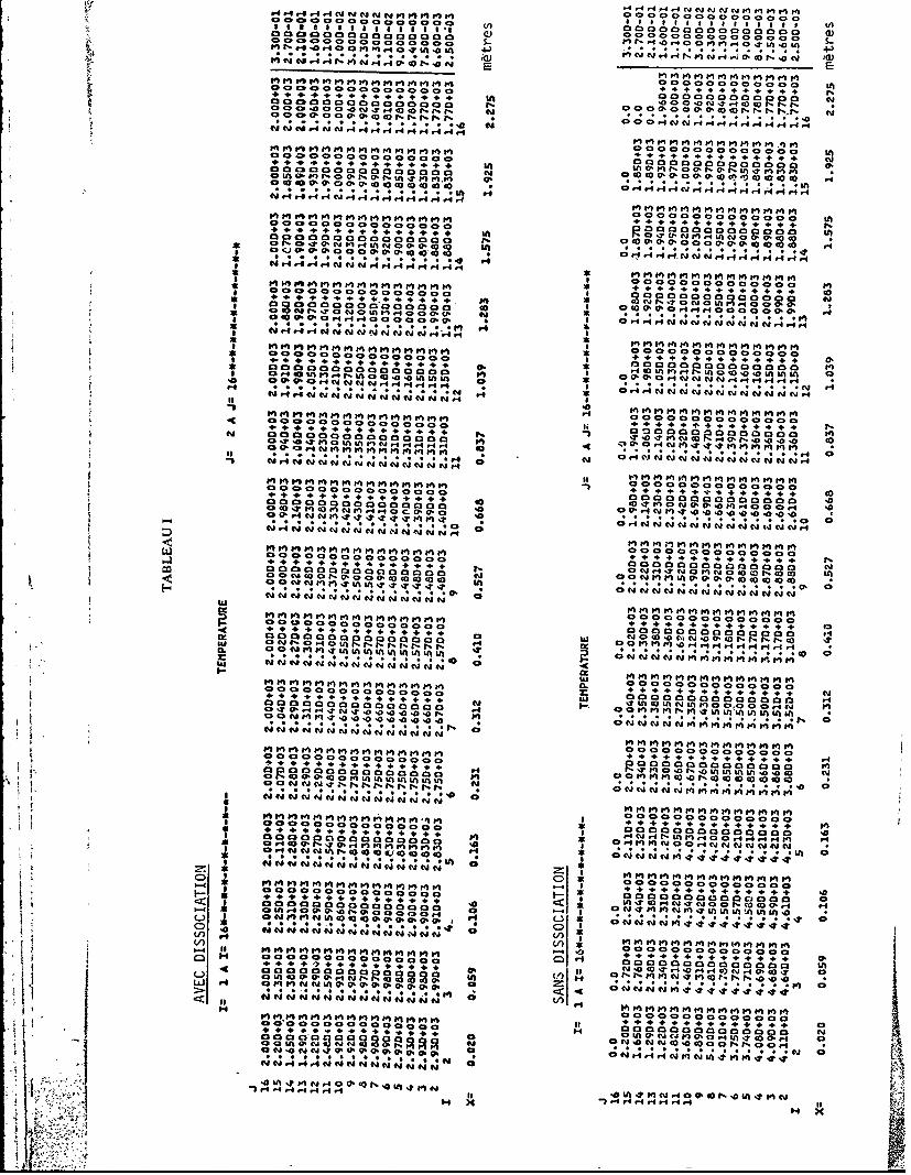
.44444N N N M M .- 4 4 4 4 W N W N W M M M M M

C, C CP 0 C3C,. K -14 4 0 A C, m

+ + 0 . . . + .00000090000 0 LA0 A O~ 400 0 0000000 000 00 000 CdciI Dc40 '34 44 4 44v4 .0 -. rr o1 1 IA

. . .

+ + .*+ LCd 0e ca N3 a 0 04.0 aa 00 0 ed . C o. 1

r.- m 0 (Y.'N. . N tn 'T a, .M .

0..00 0 0!t 0 0 40 00 00 *4 O4A.4 HW44r414.4 4 Hk 4 44Cd..,W .4 4

4..p .4..4 Hg H W

A 4 ,4 I N Oo -rot r4

0. oft M M M MT Q 5 0000000000000 0 I

0~~ C.A0a 30

A 4.4 4 ClC4 e4 N4 44 4 V; M.4*~ ~ ~ ~~~ 00. ~ .4 4 4 o 0 G 0 a m C3, 0 a N2 a a N N N 3.40 4.m

*................* .4 144 n4 A o cl-000UIvwl0 .1 -

CAo0.0 o o .0of r4 N o~0..4 N NW ri N 4 el NW 4 '44 ;-*0 O .0

C 4 NNC.4 4 4 4. . r4

4 00000000000000

A. a a oo oo0 "= N(Y0, 0 o 00 M i

*p! 0I 4 N e N e MC4 NN4 4,0MA MM A M A M A A c

0

0- 4D W M.o a W0.C.0,.0.o0

W3, N C "C n ' ANN rr' I T N Cl l N N NW l l Ci"t l

003000000000000MMII MIA MMI MMI MM 444 *~ . ,.,cc0 0 0 0 0 0 0 0 0 0 0 0 0 0 0 0 A d D0 -~ 00 NO-M *44 4444 4, . 4, Nr.N 04l .. q - 1o~ ~~~~~~~~~O..~MdO 505 eammZU At Ai nI AAlI t jV 41 41 4P ;1 4QxC;

N N W N W N W

aw Q .4C 3a0C ooooaao r.0000000 ... j-2L DIAC nm0 ) C j In 3 0 a o o D o n m m N M i in v n. n iC2 4)0 4,,r 4 . NN

C! NWN :iNNN ' -1 11 C N ; 40 0,N4 44W4,1

C00 0 0 0 0 0 Cd aN30 4 o C .Ca Cin in rl eq m " fn in n 0

n~~MM M MM IA IA1 : C M MI

tq P qp . . . . ...

. +

000000C300 I00000000000000w"t, 400000000000000 go g

A 00 0000000000n m , MIFAN o

0 42 0 N14I 4D 0 0 co0 C3 5 0 c

* . .* + . + + .<W N N N N W N W.3 0 0 0 0 0 a0 0 0 0 0 0 0 0 0 0 0 0 0 0P-4 ~ ~ ~ ~ ~ ~ ~ ~ ~ ~ M .MMc(..O O I4q r .c . M Sm WA MIAIA WMM~~W fL 0cie INMI MI M I MI M I W t4 . ~ , . * ,~- ~

00000C00 0;kn V)4 . '~o 0 0 4~

40 00 3,C0 caC 4C0 00 ca 00000000000000 In. +. .+ +*+4+4

W 44 * OI0 17W 4 D 14 4IA 0-. .4 0AOA' NW co

N0 0 :

.C Q-0140.. M

<,,.,.', '.4 Q jNr nMMM141 n1 nP

0 D .0 3 D o aC a

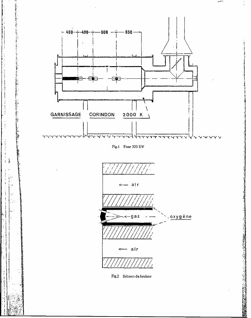
GARNISSAGE CORINDON 2000 K

Fig. I Four 300 KW

-<-a <oxyg~ne

I-IT1IFig.2 ScIhern-i du bruleur

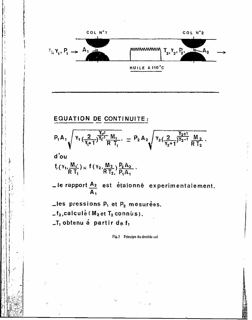
COL N1COL N*2

p f'~ " ~ \ T 2 9 2 ' h 2k.

HUILE A1100C

J EQUATION DE CONTINUITE:

Y ~12 +1PYA,2) Yi-.. MI P2 A2 Y2 2 )Y2.t -1 -- 2-.1j 1 R T2, R Td'ou

R T, RT2, P1A1

-l..e rapport A2 est etalonne' experirnentalement.A,

..ies pressions P1 et P2 mesurees.

-la f2 ,ca Icu I;(M 2 et T2 con nus)..T obtenu~ partir de.f1

I a Fig.3 Principe du double col

Uf

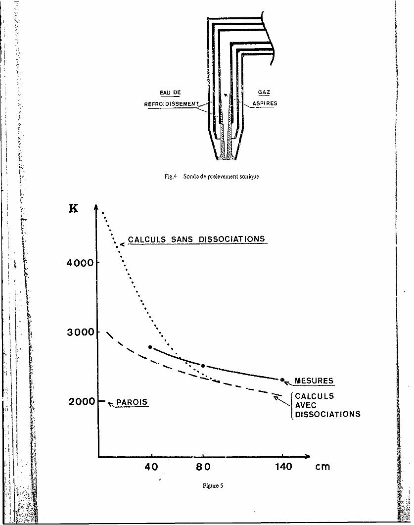
EAU DE GAZ 4

REFROIDISSEMENT- .ASPIRES

Fig.4 Sonde de prelevement soniqm~

.0CALCULS SANS DISSOCIATIONS

4000.

3000 ~ 5

S0

2000 I~2J~MESURES

40 80 140 cm

Figure 5

W DISCUSSION

E.Perthuis, FrLes calculs et expdriences mends par les auteurs ant-uls permis de mettre en 6vidence l'intdt d'un faible facteurdmissif de la flamme et des gaz dans ce four dont los parois sont tr~s chaudes?

I Rdponse d'Auteur11 aurait fallu ddcrire dans le dMail los variations des propridtds dmissives des gaz en fonction de la tempdrature etdes concentrations. Le mod~le de Salooja et Lockwood est basd sur une mdthode perfectionnde de flux avec 4 gazgris comme principe de simulation. Un des confdrenciers prdcddents a indiqu6 que cette mdthode donnait desrdsultats presque aussi bons que des mdthodes; plus sophistiqudes basdes sur la rdpartition spectrale. Cependant, iine faut pas dire que les pertes par rayonnement sont ndgligeables; elles sont importantes; et influent sur le profit detempdrature en raison des niveaux de tempdrature beacoup plus dlevds qu'i l'habitude.

J.B.Michel, NePour commenter la question prdcddente sur l'effet de l'dmissjvitd moyenne des gaz de combustion sur le caocul durayonnomont avec tempdrature 6levde do la charge, il faut dire quo cet effet n'est pas tr~s important avec desflammes of lo comburant est do l'air (e = 0,15 A 0,20) mais ii est assez important pour des flammes A l'oxyg~ne pur

t et P'on ne peut pas ndgliger la variation de l'dmissivitd avec la tempdrature.

Rdos dAtuA titre de commentaire, ii faut prdciser que la mdthode n'utilise pas la valeur (TF)4 mais 7P calculd i partir duniod~le probabiliste de Salooja et Lockwood.

N.Peters, GeNous avons fait des expdriences sur des flammes enrichies A1 l'Oxyg~ne et rnesur6 los NOx. On a trouvd des niveauxinfdriours A ceux attendus si on utilise des formules simples pour calculer ces niveaux dni NOx.

Pour des flammes alimontdes en air prdchauffd, on constate le mdme phdnom~ne. Nous pensons quo cola est dft aurayonnement tr~s important, dans ce type de flamme. Pouvez vous dvaluer le pourcentage d'dnergie rayonnde parla flanime?

Rdponse d'AuteurCes pertes, tr~s variables suivant la position dans le four, sont en moyenne do 20%.

AN EFFECTIVE PROBABILISTIC SIMULATION OF THE TURBULENT FLOW AND COMBUSTIO N UISYMMETRIC FURNACES

Th.T.A. Paauw, A.J. Stroo, C.W.J. van KoppenLaboratory for Thermal Power EngineeringDelft University of TechnologyRotterdamseweg 139ADelft, The Netherlands

ABSTRACT

The conservation equations governing the flow field and the combustion process in isothermal and in dif-fusion controlled combusting confined flows are solved using a numerical finite difference technique; theresults are compared with measurements.

The combustion process of the hydrocarbon fuel has been modelled by using instant reaction with fluctua-tions in the mixture fracture, and with three different assumptions for the chemical conditions: frozenchemistry, equilibrium chemistry and partial equilibrium chemistry.

Attention is paid to the formation of nitrogen oxides, and it is shown that in hydrocarbon diffusion flamesa substantial amount of the NO formed is due to 'prompt NO' formation. For this process an effective modelis presented.

1. INTRODUCTION

During the last decade considerable effort has been devoted to the modelling of furnace phenomena.In general two distinct lines of approaching the problem can be observed.Some authors have tried to model the furnace by dividing it into several separate sections, each

representing a simple system, s.a. well stirred or a plug flow reactor [1 1 . Although such methodsare useful for the prediction of the trends in furnace behaviour or pollutants formation, additionalmodel assumptions and empirical data are often required for particular calculations.On the other hand methods have been developed that simulate the furnace performance in more detail,generally by solving the conservation equations in finite difference form [2-4 1. These methods leadto a fair prediction of the influence of furnace geometry and configuration dependent phenomena s.a.furnace heat transfer and flame furnace wall interaction. However, these more sophisticated modelsalso require some assumptions, normally regarding the turbulence model, the radiation model and thecombustion model.In the present work such a detailed method i5 used for the prediction of the completely diffusioncontrolled combustion of gaseous hydrocarbons in an axisymmetrical combustion chamber. Several com-bustion models are investigated, all based on instant reaction combined with scalar fluctuations.The main scalar being in this case the socalled mixture fraction, and particularly, attention is paidto the accurate prediction of the fluctuations of this scalar.In this framework the mixing process of a scalar and the production of scalar fluctuations in anisothermal combustor geometry is firstly investigated by comparinq the results of numerical calcu-lations with extensive measurements by BECKER (5-6Furthermore, the assumptions concerning the combustion process are investigated in a detailed com-parison between experimental and numerical data for natural gas flames.Finally, the developed models are tested by comparison of calculations with measurements obtainedin the Delft furnace for a low NO burner geometry.

2. MATHEMATICAL AND PHYSICAL ANALYSIS

2.1. Basic equations.

The calculation procedure consists of solving the partial differential equations representing theI conservation of the time averaged flow properties in an axisymmetrical flow geometry. The general,elliptic form of these equations can be expressed as:

(pu¢) W+ (pvr) (P r + Sax-r(3rBx aBx r 3r *Br(1

in which u and v represent axial and radial velocity, and * a flow property, with p as its viscosityand.S as its sourceterm.

In the case of furnace calculations * represent subsequently (u, v) axial and radial velocity, (k, e)

the turbulent kinetic energy and its dissipation, h, the stagnation enthalpy, ( , R ) the radiant

heat flux in the x and r direction for radiant gas k, (Yf, Ye), the mixture fraction and its root

mean square, value and finally YNO' ,the mass fraction of therMal NO.

The values of y P and S are given in table I. Constants necessary to solve these equations are

given in table II.When no recirculation takes place, as in-the case of free diffusion flames, the second form on theright-hand side of (1) can be omitted, transforming the partial differential equation to a parabolicform, which is easier to solve numerically.For the solution of equation (1) it is necessary to define boundary conditions; at the axis of sym-metry tr = 0) thesp are: v = 0 and a /Br = 0 for all other quantities, at the solid boundary empiricalwall functions can be used to relate (B$/Br) to the local values of €, for u, v, k, C and h [2, 7 1,

k, kand for [x R 8 1; the other values of * are set to zero. At the exit of the duct and furnace cal-

culations (B /Br) was assumed to be zero, and at the entrance all variables *were specified.

-1 ~'

2.2. Turbulence model.

The two-equation turbulence model used in the present work is based on the solution of the equationsfor the turbulpnt kinetic energy k and its dissipation rate c; in this model the logic assumption forthe turbulent viscosity is: ve = C pk2/c. This viscosity has to be added to the laminar viscosity.

e DThe chosen model had been shown to give good predictions in boundary layer type flows [9 ], and alsoin more strongly elliptic flows of the same geometry as has been used here [2, 10 ]Because of the uncertainties in the combustion model more refined turbulence models are judged to beover-sophisticated at this stage of the development.

2.3. Radiation model.

The four-flux radiation model adapted here is based on the formulation of GOSMAN e.a. [8 3 , which

reduces the original four equations for the radiation fluxes in four directions, Ik and Ik forx+ r+k k k

radiant gas k, to two equations governing the distribution of the sum parameters R = (I + 1)/2,an k. AadRr= (Ir+ + Ik_ )/2. Although this formulation is efficient a deficiency can be the uncoupling of

r r+ rthe fluxes in radial and axial direction.Nevertheless summations of radial and axial f: "'4s, representing fluxes in directions under 450 withthe symmetry axis, are evidently coupled. Also the dependency of pRk on r correctly represents the

rconsequences in radial direction of an anisotropic flux distribution.Moreover the physical constanti to be applied to the scattering and absorption of the calculus areuncertain, not at least because of the occurrence of luminous radiation.Therefore scattering has to be assumed negligible, and two models for the absorption and emissioncoefficients have been tested. In a first model the absorption and emission constant have simply beenchosen conscant (al - cl - 4), representing a one gray radiating gas. In a second model the constantshave been assumed to be temperature and mixture dependent (ak (Y , Y , p, T) and

(YC0 , YH20, p, T) for gas k) in a one clear, three gray gas formulation for natural gas developed

and used by the IFRF [11 1 for natural (Groningen) gas in similar calculations.

2.4. Combustion models.

In the literature concerning combustion models two categories of models have been proposed. Thefirst category consists of models in which the governing parameter is the fuel mass fraction. Theconservation equation for the fuel mass fraction is solved using an effective source term, beingeither an Arrhenius type reaction rate or a flow pattern dependent reaction rate, s.a. the eddybreak-up rate proposed by SPALDING [2 1 or in a different way by BRAY (12 ]. These models seem tobe particularly suited for modelling premixed flames because there the effective reaction rate isthe controlling factor.In diffusion flames, however, the mixing process is much slower then the chemical reaction. Conse-quently the combustion process is controlled by mixirg, the reaction rate can be assumed as infinitelyfast, and a parameter like the mixture fraction, d6ailning the mixing process, controls the reaction.The relation between the reaction process and the mixture fraction in this case can be found via thequantity:

f = rYfu - Yox (2)

where Yfu and Yox denote fuel and oxidant mass fractions and r is the stolchiometric mass ratio

between fuel and oxidant.The conservation equation governing the distribution of f has a source term equal to zero. Further-more the following identity can be deduced:

ox flu fox(3)f f ffo

where Yf in the fuel phase is equal to one, and in the oxidant phase equal to zero.At the stoichiometric conditions: s = 0, and Yf = 1/(r+1). For the Groningen natural gas usedin our experiments r = 13.07 and Yf = .071.

So far we have made nu proposals for the reaction process, beside the fact that it is slower than themixing process. In the paper threemodels will be discussed: the well known frozen composition model12 ], the equilibrium composition model and a so-called partial equilibrium composition model.

2.4.1. Frozen composition model (model 1).

In this model it is assumed that the infinitely fast reaction is restricted to an infinitely smallreaction zone, situated at the surface where Yf,= Yfst Outside this reaction zone the reaction is

considered to be completely quenched, ard the composition is in effect frozen.Under these assumptions it is a simple matter to define mass fractions and temperatures, for example:

Y fu 0 for Yf <Yfs

and

Y =0 for Yf > Yf (4)Yox Sst

The respective Yox and Yfu can be found by means of equations (2) and (3). The temperature is cal-

culated with help of the calculated enthalpy and an average value of the specific heat. The densityfollows fro. the equation for a perfect gas. Curves for the temperature and the oxygen concentrationunder adiabatic- conditions are depicted in figure 1.

I2.4.2. Equilibrium composition -mcdel (model 2). 6

In this model it is assumed that the infinitely fast reaction is not restricted to only a reactionsurface, but does occur in the whole field, both for forward and backward reactions. This resultsin a local equilibrium composition, governed by the local equivalence ratio related to the mixturefraction and the local enthalpy. In this case it is not possible to obtain a straight forward rela-tion between the relevant properties (e.g. the temperature) -and the mixture fraction and enthaipy.

To avoid this difficulty the following procedure has been adopted (14 1. A two-dimensional mappinghas been made of all relevant thermodynamic and chemical properties: temperature T, density p,viscosity V, and mass fractions YC ,' YCO , H ' and YO.Y02' 4 C02 CONH20' Y H2 ' 0Using a least square method, thismapping has been fitted in Chebyshev double polynomials:

I JY (h - E E ajTi h ( (5)i fhX)-~. ~ f

* .* =

in which h and Yf denote normalised values of h and Yf, whereas Ti denotes a Chebyshev polinomial of

degree i and I and J have values up to eight.Equation (5) represents an efficient instrument for the calculation of the equilibrium conditions,when the recurrence relations for Chebyshev polynomials are used. However, in the iterative procedureto solve the finite difference form of the partial differential equations, mentioned before, a muchmore economical prodecure is employed by making use of the mentioned two-dimensional mapping employingbilinear interpolation. Also in this case calculated curvt s of T and Y02 are given in figure 1 foradiabatic conditions.It should be noted that the temperature sharply decreases at the rich side of the stolchiometricpoint; the decrease coincides with an increase in Y and YY~H2 YC

2.4.3. Partial equilibrium composition model (model 3).

In figure I experimental data obtained from mass fraction profiles, measured in attached turbulentnatural gas diffusion flames (14 ] are also reported. From these results it appears that the equili-brium composition assumption gives temperatures that are too low, while the frozen composition tem-peratures are much too high. More surprising, however, are the molecular oxygen curves. Theoreticallythe 02 mass fraction at fuel rich condition (Yf > 0.071) should be essentially zero both in the frozen

and the equilibrium condition and even taking into account the unmixedness the highest value forY to be expected below near stoichiometric conditions (Yf = .11) is 1.5%, whereas values beyond 5%02are measured.Obviously nearly all fuel (ma, nly CH4) is consumed, but due to the short residence time in the flamefront only part of the 02 has reacted, resulting in high CO en H2 mass fractions.Behind the flame front the further reaction of 02 is apparently suppressed and a frozen compositionis found but with a finite 02 mass fraction.The reason, for the quenching lies in the fact that in hydrocarbon flames 02 mainly reacts with Hradicals, and as shown by BULAU a.o. [18 1 the OH, H and 0 radicals effectively almost fully recom-bine for * > 1.65 (Yf > .088).To take these effects into account a partial equilibrium hypothesis io introduced, stating thatoxygen in the fuel rich region does not react and so gives a constraint. The other species concen-trations and the temperature have been calculated based on an equilibrium assumption with the con-straint 02 concentration. In figure lb this hypothesis is illustrated by a straight line tirough themeasured data points and gives a value at Yf = Y of Y 4%.

f f I Of 02The calculated equilibrium temperature curve following from the quenched equilibrium hypothesis,using this Y constraint, is drawn in figure la and is seen to compare favourable with the measuredj data. 02

On behalf of further flame calculations the most relevant species and thermodynamic properties werecalculated for quenched equilibrium conditions as functlon at the enthalpy and the mixture fraction,and also transformed in Chebychev polynomials in the way, explained in section 2.4.2;

2.5. Nitrogenoxide formation model.i ! In diffusion flames it is often assumed that most of the nitrogenoxide is found by high temperaturereaction between oxygen and nitrogen molecules and atoms. This so-called thermal NO formation is

usually based on the'Zeldovich mechanism, with reaction rate:

N2 f YO (Yf)*No (Yf) 0kz exp (-E/T(Y)) (6)

Iwithk 10.11.15 and B =37.10 MN2 and MO denote the molecular weights. owith kz • z o

, r?'o-0,

The atomic oxygen mass fraction may be calculated either by the assumption of chemical equilibriumbetween molecular and atomic oxygen for the frozen chemistry models or by using equations like (5)for the equilibrium, chemistry models.In calculations for natural gas diffusior flames we found that especially for the equilibrium modelsthe calculated thermal NO mass fraction was much smaller than the measured NO mass fraction. Thismay tndicate that 'super equilibrium' oxygen concentration (see 2.4.3) play a role. Another possibleexplanation is 'prompt NO', often neglecLed in diffusion flames studies. As 'prompt NO' is formedonly inside the reaction zone a frozen flcw composition description for calculating the additionalformation of thermal NO can be used. To test this last assumption measured NO mass fractions in at-tached natural gas diffusion flames are plotted against the mixture fraction in figure 2. This hasbeen done for several values of both the Froude number (Fr = u2/gD, with burner velocity u and burnerdiameter D, representing the influence of buoyancy fcrces on the flame and the Damh6hler number (Da =

-5(D/u)/Tcr, with Tc as a critical combustion time, chozen here to be 5.10 s, the characteristic blow-

out time of a homogeneous reactor), representing the xnfluence of shear on the reaction process. Fromfigure 2 it is clear that a correlation between Y and Y does exist. The "too low" experimentAl NO

NO fvalues on the fuel richside can be explained by the fact that 'prompt NO' is partly preceeded by HCN125 1, not measured here. The higher values of NO for fuellean mixture can be explained by the in-fluence vf additional thermal NO. The introgenoxide mass fraction at the stolchiometric Yf value

(O =O 38 ppm) compares well with the 'prompt NO' concentrations measured in premixed stolchiometric

hydrocarbon flames [19 ]. The thin line in figure 2 drawn to ough the full circles represents aslightly lifted flame (Xign/D = 3.5). It is clear that in this case the constrained, unreacted oxygen

did not produce NO and the correlation mentioned above and drawn in figure 2 has to be changed, usingthe Yf value of the ignition-point. In the following calculations both the thermal NO formation and

the frozen flow 'prompt NO' contribution have been determined and added to give a total NO massfraction.

2.6. Probability formulation of the mixing process.

The usefulness of t probability description of flames is illustrated by figure )a where small fluc-tuations in Yf around the stolchiometric value result in large fluctuations in temperature, especi-

ally in the case of the equilibrium models. By reverse it is evident that momentary temperatures canbe much higher than the average temperatures, resulting e~g. in instantaneous reaction rates that areorders of magnitude higher than those based on the average temperature.Time average flow properties, the spatial distributions of which prescribed by equation (1), can bereaveraged as moments of the probability density function (PDF) governing the time dependent behavi-our of the observed property. When a gaussian PDF is assumed tha first and second moment of the PDF(representing the mean value and the root mean square value) completely determine the PDF. In ourcalculations such an assumption has been made for the PDF of the mixture fraction; the fact that Yfcan not be lower than the oxidant value or higher than the fuel value being taken into account by

the use of a clipped gaussian shape, following LOCKWOOD e.a. 1 20 J. From the PDF for the mixturefraction, P(Yf)s the PDF for the temperature: P(T) can simply be derived by putting:

P(T)idT - P(Yf)IdYfl (7)

The contributions to P(T) above and below the stolchiometric value of Yf have to be added. In figure

3 measurements of P(T) in natural gas diffusion flames (15 1, around the stolchiometric reaction zoneare shown and compared with the results of calculations. Each calculated curve is based on 16 points,

(smoothed histograms, being composed of 16 bars) obtained by using calculated Yf and Y-12 (= Yf')

values and assuming a clipped gaussian PDF. Also here it is clear that the partial equilibrium flow,gives the better results by imposing a certain upper temperature limit (T - 1900 K) much lower thanthe adiabatic value (T = 2210 K).Using equation (5) representing the combustion models and a Schwab-Zeldovich coupling function be-tween h and Yf [21 : h = O(Yf) and assuming that the Lewis number unity, the mean concentrations for

the chemical properties can be defined by:HJ1 Y d (8)M Y 1f1), Y f) Pf) df18

CH4 , H20, H2 CO, CO2 and 0. The same procedure is followed for the physical pro-

pertes T, p and ji and for the !prompt, No', where the linear relation drawn in figure 2 (thick line) A

has been applied to determine YN-(Y

The formation of thermal NO is governed by the averaged source term (6):

-wN° f *No (Yf) P(Yf),dYf (9)

source terms for the four flux models are formulated as:

CkT4= f Ck (Yf) T4 (Yf) P(Yf) dYf and

50

1

a = f ak (Yf) P(Yf) dYf (10)

In (9) and (10) it is anticipated that the temperature, density and concentration dependencies can beexpressed in a mixture fraction depencency.

2.7. Solution procedure.

To solve differential equations represented by equation (1) and table I, these equations are ex-pressed in finite difference form and solved by the algorithms for the elliptic case and the pa-rabolic case as given in respectively [22 1 and [23 ]. The calculations for the elliptic case were performed with a 20 x 20 nodes grid geometry. The numberof iterations required to reach the convergion criterion defined in [22 1 was 300 in the case ofisothermal confined flow. For the free jet diffusion flame with a simple model for the absorbtion andemission coefficients it reached 600 and for the case of more elaborate radiation constants, up to1000. This same number of iterations was required for confined combustion calculations. The use of acombustion model led to an increase of necessary computing time per iteration with a factor of twocompared with isothermal flow calculations. The elaborate radiation model led to an increase with afactor of turee. The parabolic Lcheme for the free jet diffusion flames calculation was two orders ofmagnitude faster than the elliptic scheme however.

3. RESULTS AND COMPARISON WITH EXPERIMENTS

From the previous paragraphs concerning the combustion models and the introduction of the PDF it isclear that the mixture fraction and -its fluctuations play an important role in the calculation pro-

i cedure.Mostly t e stochiometric value of the mixture fraction is small (nat'ral gas: Y 0.071) which

Mosty t~e soichometic f'stmeans that small variations in the gradient slope of the axial Yf profiles result in large variations

in the predicted temperature curves. Confinement and recirculation strongly influence the accuracy ofthe prediction of the mixture fraction field and therefore the elliptic program was first tested forisothermal confined jets. Subsequently unconfined diffusion flames have been calculated with both theparabolic and the elliptic program in order to test the accuracy of the letter program and the in-fluence of the grid arrangement, and for the comparison of the combustion models with experiments. Atlast comparison is made between furnace calculations and measurements.

3.1. Confined isothermal jet calculations.

To verify the equations that govern the mixture fraction and its fluctuations in a confirmed flow wedecidd first to compare calculations in isothermal flow with measurements. The only available expe-rimautal results in cenf1.aed jet flow providing information about the mixture fraction and its fluc-tuations are those of BECKER [5 ], [6 1, [16 ].

4The results also concern detailed measurements of the mean flow pattern and the static wall pressure.p The data have been obtained in a cylindrical duct (.197 m diameter, 1.25 m length, smooth wall), in

the center of which an air jet initial velocity u (uniform profile, 6.35 mm diameter) was situated,

surrounded by a secondary, uniform ground stream (velocity uw,o).

The calculations have been carried out for different combinations of primary and secondary velocities,yielding Craya-Curtet numbers of 1.22, .673, .345 and .212. These numbers correspond to flow patternswith increasing recirculation. The Ct number is defined as:

h t - with u*2 = uf2 Cu2. +

where ; and u2- are the area-averaged velocities (5 1, and u*2 can be regarded as a measure of the

non-uniformity of the momentum flux distribution at the inlet.The ducted flow can be regarded as being devided into three regions: a region of jet growth, a re-circulation zone, and post-jet mixing zove. This becomes particularly clear from the axial profilesof u /(u-u ) and Yo/(Y-Yf) given in fic;ure 4 and 6, wnere u and Y refer to the ground stream.

0 w fo ff,w w f,wThe relation between the reciprocals of mixture fraction and velocity and the axial distance islineair in the jet growth region, whereas the curves bend steeply upwards in the final region. Herethe ground stream velocity tends to the velocity at the axis. Especially for lower Ct numbers thereis a good agreement between calculated and measured data. The changes in mixing regime are also wellrepresented in the static pressure profile (figure 5) where the position of the sudden increase inpressure corresponds with- the eye of the recirculation zone. However, the absolute values of thepressure rise are conspiciously high in comparison to the measured results, indicating that over-prediction of wall friction or internal friction in the recirculation zone does ssible occur. Itshould, be noted that the pressure rise does s6sitively depend on the profile of the nozzle glow,here assumed to be essential uniform. Similar overpredictionsof the pressure are also reported byKANG e.a. [10 1 using the same meth d in confined flows wih comparable Ct numbers.The post-Jet mixing behaviour is mainly characterised by the mixture fraction fluctuations; someresults are depicted in figure 7. Beyond the recirculation zone, i.e. when the jet has reached thewall, the production of fluctuations diminishes and dissipation results in their decrease.This is reproduced in the calculations for the lower Ct numbers, allthough the maximum predictedfluctuation intensity at low axial distances are higher than those measured by BECKER [30 1. Measu-rements in free jets by Haberda show a better agreement. For rhe lower Ct numbers investigated themaximum influence-of the mixture fraction fluctuations on the temperature field can be expected tooccur in the reaction zone around Y' considering the combustion model that was applied. For natural

- - - f'stgas, Yf,st = .071, corresponds with X/Df > 15; in this region-the predictions are fairly correct.

I-=

For the highest Ct number the axial profile of mixture fraction fluctuations is not influenced by theIF confinement and resembles the calculated profiles in free jets using the same set of partial diffe-

rential equations as in table I but in a parabolic form [ 17 ], [241. In the last case the value ofit I on the axis is only slightly smaller than the value of .227 obtained here.

3.2. Free jet diffusion flames.In order to validate the combustion models described before, we decided to compare calculations forthe relatively simple turbulent diffusion flame with detailed measurements concerning the temperature,mass fractions, velocity and radiation field in such flames. For the comparison a vertical natural

-2 _gas flame with D = 10 m, u = 20 m/s, Re = 14500, Fr = 3900 and Da = 21 was selacted; because of

0

both the considerable shear stress and buoyancy in this flame no local laminarisation of the flamefront is to be expected.

3.2.1. Influence of the numerical method.

The numerical predictions for the flame have been obtained in two ways: using a parabolic flow programand using a elliptical program, with respectively a 20 x 25 and a 21 x 30 grid arrangement. The axialand radial grid locations have been chosen finely distributed around the burner, both with a nodedensity for grid II two times higher than for grid I.Presumably in this region the grid II is smaller than the turbulent macrolentgh scale whereas it isslightly larger in grid I. The results indicate that an underprediction of the prcduction of turbu-

ft lence follows from the larger grid spacing. The outer radial grid point (the wall) is situated at adistance of .5 m from the burner. Here a secondary flow with a velocity of .2 m/s is assumed incombination with zero wall gradients. Varying these assumptions within reasonable limits did notinfluence the flame structure.The mean axial temperatures calculated with combustion model 2 and the different numerical schemesare presented in figure 8. The coarse grid I obviously leads to a slower mixing process than thefiner grid II, resulting in a stolchiometric mixture and a maximum temperatuze further downstream.Using grid I leads to an upstream shift of this point both for the elliptic and the parabolicscheme. By combining the parabolic and the elliptic scheme in an additional calculation it was shownthat the influence of the grid spacing wav mainly restricted to the region between the burner mouthand x/D - 5. Using the results of the fine grid parabolic scheme in this point as initial values forcoarse grid elliptic scheme calculations further downstream brought the position of the maximumtemperature within 10% from the position obtained with a completely fine grid calculation. Theproceeding results show that for turbulent, diffusion flame-lik3 combustion processes (free jet flowor confined flow with a large Ct number) a carefull choise has to be made for the grid location inhigh intensity mixing zones. Grid spacings as given for grid 1 have been used for all the followingcombustion calculations.

3.2.2. Influence of the combustion model.

With the fine grid spacing the diffusion flaL- defined before has been recalculated with the frozencomposition and the pai tial equilibrium combustion model. The predicted temperature profiles, velo-city and mixture profiles both using the parabolic and elliptic computation scheme are presented infigure 9 and figure 10 and are compared with experimental data obtained with respectively micro-thermocouples (di&-eter 20 um), a laser-dopplur anemometer and a detailed gaschromatographic analysisr15 ]. Experimeatal probability density functions for the temperature, compared with calculated Valuesz'or the equilibrium and the partial equilibrium model were shown earlier in figure 3. For the tempe-raturns the agreement between calculation and experiment is very good for both the equilibrium andthe partial equilibrium: however the last model is to be preferred because of the better agreement inPDF values. The difference in temperature predicted by subsequently the elliptic and the paraboliccomputational scheme as shown in figure 9 for the equilibrium composition model is small and is alsotypical for calculations using the other combustion models. The main conclusion to be drawn fromfigure 9 is that the frequently applied frozen composition model leads to an unrealistic short flamelength and too high a maximum temperature. Considering also figure 3 (and figure 16) the partialequilibrium model appears to be more realistic than the equilibrium model.From figure 9 further a siall shift in the position of the predicted flame front given by the maximumtemperature is observed in comparison with the ecperimental data. This is possibly caused by inpar-fections in the turbulece model. However, optimalisation of tha chosen turbulence constants is

omitted.The axial profiles for velocity and mixture fraction presented In figure 10 show the mutual devia-tiong between the distinct numerical procedures and combustion models to be rather small for thesequantities. The difference between measurements and predictions is much larger, however, particularlynear the burner. The cause being that the flame was lifted to a height of x/D = 9 above the burnerI mouth. The agreem~nt further doin 'stream stems from the enhanced mixing by buoyancy forces, thesecausing high axial velocities around the maximum temperature region. Predictions with a somewhat moreelaborate combiscibh model, design~da.o. to predict ignition, are depicted in figure 10 by thecurves c. The agreement is very good for both the velocity and mass fraction; the temperature curvesas preseited in figure 9, do not change in the new model. More details on the improved combustionmodel will shortly be published, after completion of its development.

3.2.3. Radiation prediction.

Allthough the radiant heat trarmsfer in, the diffusion flame investigated is relatively small it providesan opportunity to test the various radiation models.Experimental data obtained with the Shell radiation pyrometer [15 1 are given in figure 11 togetherwith predictions using the equilibrium and partial equIlibrium combustion models and various radiationmodels. For the simple one gray gas model (ak = 0.4) gave a higher (radial) radiative heat transfer

than the partial equilibrium model. reflecting the fact that the maximum temperatures are higher for

Z1-1

the equilibrium model (see figure 3). The maximum value of the measured radiative heat flux liesbetween the two predicted values. The predictions based on the IFRF correlation (1 11 1, 3 gray/1clear gas, verified for natural gas only) show good agreement with the measurements. However, thecomputing time using this correlation was much higher, while the improvement of the prediction wassmaller than the influence of the combustion model. Therefore the simple radiation model was pre-ferred for subsequent furnace calculations.

3.2.4. Pollutants prediction.

The calculation of NO formation is devided in 'prompt NO' formation and 'thermal NO' formation in themanner discussed before. The 'prompt NO' values are given separately in figure 12 and appear to befairly independent of the combustion model used. However, as shown in figure 2, lifting of the flame(equivalent to pre-mixing!) influences the NO concentration. So, using the improved combustion model(section 3.22), to estimate the lift of the flame, calculations of prompt NO concentrations have beenmade both for the lifted and the attached flame. The results show that in the attached flame themaximum prompt NO concentration is found well inside the fuel rich part of the flame; in both flamesY is reached at x/D = 80. For the lifted flame, however, the maximum prompt NO concentrationf'stoccurs near the stolchiometric poJn.', as does the maximum NO concentration.The thermal NO profiles calculated for the different combustion models are also shown in figure 12.They reflect the important influen.e of the temperature on the NO formation. The thermal NO formationin the frozen composition and the equilibrium model is suostantial, because in these models theadiabatic combustion temperatures can be reached. However, the measured results from figure 3 Indica-te that the low thermal NO profiles obtained with the partial equilibrium model must be considered asbeing the most reliable. Addition of the preferred 'thermal NO' and 'prompt NO' profiles leads to atotal NO profile comparing fairly well with the profile measured with the chemoluminescent method[15 ). The shift to the richer part of'the calculated profile compared with the mt:..-rements might bedue to the fact that part of the 'prompt NO' is decomposed to HCN, not measured here. However, it ismore likely that the flame is simply some 10 D shorter than the predicted one. A similar shift isalso reflected in the temperature profile in figure 9 (curves a and b).The identified importance of 'prompt NO' is largely in accordance with the results obtained by TAKAGIe.a. [28 1 , in propane diffusion flames. In most other investigations the role of the 'prompt NO' iswrongly overlooked.

3.3. Cylindersymmetrical furnace calculations.

To test the models for furnace applications we used the extensive experimental data obtained in theDelft furnaces equipped with a newly designed central air burner (CAB) [29 1 . The CAB was designed tocombine a stable combustion process, with easy dual fuel burning and low NO formation. The basic ideais that introduction of the gas through an annulus around a cylindrical airJet leads to a smalleffective hylraulic diameter of the gasflow and consequently to flames with a short reaction zone, alow residence time in the reaction zone and a low total NO formation. Calculations were made to testthis hypothesis. Moreover several additional calculations have been made using central gas burners(CGB) in order to investigate the influence of scaling up of the furnace on NO formation.

3.3.1. CAB calculation and measurement.

The CAB calculations concerned a CAB, burning Groningen natural gas with a capacity of .75 MW, at anoverall equivalence ratio of .98, and producing a flame essentially attached to the burners.The main dimentions of the system are: primary air stream, diameter 95 mm, width of annular gas slot6 mm, furnace diameter 0.6 m, length of (horizontal) furnace 5 m. The walls of the furnace are cooledto about 350 K by means of water.Gravity effects have been neglected because no influence of buoyancy was detected in the experiments.The initial velocity profiles are not known, but aerodynamic resistances (wire mesh in the gas flow,perforated plate in the air flow) are applied to make them uniform. The furnace walls (estimatedemmisivity = .8) are water cooled and have been assumed to be smooth; the short chimney at the end ofthe furnace is replaced by sudden enlargement, for reasons of simplicity.Following GUNTHER [32 ] we define the radiative heat transfer in the furnace with the dimensionlesshcTHRING number; Th = - where n is the mass flow, h the specific enthalpy for a stolchiometricSqrc cnatural gas-air mixture, (hc = 2.8 NJ/kg), S is the furnace wall surface and 4 the radiative heat

c rcflux calculated with the adiabatic flame temperature of natural gas with a emissivity a - .4 (4 -

.53 MW/i 2 ). The THRING number is often referred to as the reduced firing density; in our caseits value amounts to .3.For the convective heat transfer and for similarity in the gas flow the CFAYA-CURTET number, definedbefore, and the burner Reynolds number have been applied as similarity parameters, following KANGe.a. [29 1. The numerical values are Ct a .18 and Reb = 2.105 (Reb refers to the air flow).The axial temperature and NO mass fraction profiles together with experimental data are presented infigure 13. The substantial difference between the predicted and measured temperature profiles thereby

suggesting an unrealistic forward position of the flame. The two combustion models as such lead tolimited differences in the predicted temperatures.It has often be observed that the pyrometer tends to stabilize the flames, presumably due to the 2.5cm diamwter suction pyrometer used for the temperature measurements.As for the calculated NO mass fraction profiles agreement results between the results of the partialequliibrium model and the measured YNO profile is striking, apart from the axial shift mentioned

earlier. The calculated thermal NO contribution is very small ( > I ppm for the partial equilibrium,and < 3 ppm for the equilibri , moadl; consequentily n~arly all NO predicted is due to 'prompt vol).The differences in the temperature profiles are reflected in the predicted heat flux profiles at thefurnace wall (see figure 14), most notably downstream of x/Df = 3. However, for both combustion

Smodels the total local heat flux corresponds fairly well with the measured values (determined with anapc'uv'acy of - 3% from the heat balance of the water, cooling the distinct wall segments). f

t WF

The res ults of separate measurements of the radiative heat flux, using an ellipsoidal pyrometer andthe predicted radiation are depicted in the lower curves of figure 14. The discrepancy betweenmeasured and calculated radiative heat fluxes is not clear and is possibly due to an incorrect angledependent sensitivity of the useJ pyrometer.The large contribution of the convective heat transfer to the total heat transfer particularly nearthe maximum, should be noted.The double peaked value of the total heat flux found with the partial equilibrium model is due to twopeaks in the convective heat transfer curve. From these and other calculated data it appears that thedip in the heat transfer curve as X/Df = 3 occurs at some distance beyond the end of the recircula-

tion zone. This position corresponds well with the end of the recirculation zones that was calculatedto be situated between X/Df = 2 - 3 for isothermal flow and Ct = .212 - .675 (figure 5). 4

The first peak can be traced back near the point of reattachment to a high value of the turbulentkinetic energy. This higher turbulent level leads to heat transport to the wall. The second peak isdue to the maximum in the temperature of the gas near the wall, occurring some distance beyond thereattachment point in this case.Further support of the reliability of our predictions of the excessive heat transfer around therecirculation zone was obtained from experimental data of KRALL e.a. [30 ]. Calculations for a geo-metry similar to his experimental setup and at Ct number within the experimental range (.25 - .66)resulted in the same sharp increase in heat transfer in the recirculation zone as observed [31 .

The quantitative agre.ment between Kra.'s measurements and our predictions was satisfactory, in-dicating that the calculation method is well founded.

3.3.2. Influence of furnace size on NO formation and flame length.

Because the prediction metod of NO and the wall heat transfer has been shown to give realisticresults for smaller furnaces, some scouting calculations were made to test its applicability forlarger furnaces dimensions and furnace loads. The calculations were restricted to the verticalcylinder symmetrical open ended furnace.The similarity parameters were kept constant at Ct = .18 and Th = 3; these values being chosenbecause of their frequent occurence in real furnaces.As for the burners tho primary gas flow diameters were taken at .03, .09 and .27 m, and the burnerloads at 1.9, 17.1 and 155 MW. The overall equivalence ratio was taken equal to .96 and the gasvelocity e ual to 75 m/s in all three cases. The corresponding burner Re numbers are 2.105, 18.105and 160. 10. The velocity in the annular streams of air surrounding the cylindrical gas stream wasset at 25 m/s.The predicted mean 'thermal NO', 'prompt NO' and 'total NO', concentrations at the furnace outlet aregiven in figure 15. The furnace size is characterized by the parameter Dh/% (Dh- hydraulic diameter

of gas flow, ub = m-an flow velocity at the burner); for the geometrially similar furnaces considered

this parameter is proportional to the residence times of the gas in the flame zone and in the furnaceas a whole. Relating the parameter to the chemical reaction rate yields the earlier defined Damk~hlernumber.From the results it can be concluded that for the burner and furnace dimensions investigated, most of

the NO formed is 'prompt No'. However, D,/a > 1.5 10 , which corresponds to Da > 200, the 'thermalNO' formation becomes dominant.The calculated flame length, being defined as the distance between the burner mouth and the pointwere the maximum temperature is reached and nearly all fuel has been burncd, is shown in figure 16and compared with several data obtained from the scarce literature.

The flame length for large vertical enclosed diffusion flames might become a more important parameter,in the future due to the tendency to build more furnaces using bottom fired large diffusion flames.With an ensemble of these slender well defined times it is easier to exploit the available furnace~volume optimally, than with strongly swirling flames [ 34 ] .It is clear from figure 16 th?.t the calculations show the same trend as the measurements quoted by

GUNTHER (32 1 and NIEPENBURG (34 ]. Yet the predicted flame lengths are considerably larger; this maybe due to the fact that weak swirl is often applied in the measured practical flames. The calculateddata points can be matched with the correlation:

L = .21() 0 "5 , where L stands for the flame lengths (in m) and Q is the burner load (in MW).

CONCLUSIONS

From the presentea comparisons between measurements ans calculations, a number of pertinent conclusionscan be drawn.

1. Out of the presente.d combustion models for niatural gas diffusion flames, the so-called partial equili-biitm composition model gives the best general agreement between theoretical and experimental results.

2. The equilibrium composition model might be satisfying for the prediction oZ the mean flow and tempera-ture field, but it predicts too large temperature fluctuations and too high instantaneous temperatures;consequently it is less suitable for estimating the temperature dependent NO formation.

4 3. The freoaently used frozen composition model clearly leads to erroneous results.

4. It can be expected that the partial equilibrium conditions depend on the turbulent stretch in the f£qw,but mea,,urements in natural gas flames with different stretch levels [ 15 1 , characterized by Da - 2-200,reveal that in practical diffusion flames the influence of stretch is very small. Because of the nigh

2 I hydrocarbon content of Groningen natural gas, it 6an be anticipated that these conclusions are gene-I rally valid for hydrocarbon flames.

5. Further it is found that the thermal NO formation in non-preheated hydrocarbon flames is relativelysmall, parlicularly for the small and medium size hydrocarbon flames used in experimental studies. Onthe contrary the contribution of prompt NO is particularly relevant; its formation is satisfactoxymodelled in our study.

6. When 5nterpreting NO data in diffusion flames one has to be carefull when dealing with lifted flames.In that case the NO mass fraction profiles in the fuel rich region derived from prompt nO formationcan be changed completely, due to premixing with air.

7. Taking into account mixture fraction fluctuations, calculations using the k-c-turbulence model havebeen made for isothermal furnace flows; the results were found to be in general agreement with expe-rimental data [5, 6 1. Subsequent furnace calculations show a very good agreement between measurementsand calculations for the NO mass fraction and the total wall heat transfer.

8. Further the calculations lead to the conclusion that in the slender cylindrical furnaces investigated,characterised by Th = .3, Ct = .18 and Re = 2105, the contribution of convective heat transfer domi-bnates in the total wall heat flux particularly in the recirculation zone.

9. The parameter study finally shows that the applied numerical technique is well suited for the predic-tion of the influence of furnace size and proportions on such quantities as NO formation, flame lengthand heat transfer. However, further validation of the method is required in this field.

ACKNOWLEDGEMENTS

The authors like to acknowledge the cooperative support provided by prof. D.B. Spalding and dr. A.S.C. Maof Imperial College, London in arranging the basic computer program used in the present calculations anddeveloped by Combustion, Heat and Mass Transfer Ltd.

REFERENCES

1 OSGERBY, I.T.,Literature Review of Turbine Combustor modeling and emissions.AIAA journal, 6 (1974), p. 743.

2 KHALIL, E.E., SPALDING, D.B. and WHITELAW, J.H.The calculation of local flow properties in two-dimensional furnacts.Int. J. Heat Mass Transfer, 18 (1975), p. 775.

3 HUTCHINSON, D, KHALIL, E.E. and WHITELAW, J.H.The calculation of wall heat transferrate and pollutant formationin symmetric furnaces.4th Members conf. IFRF, paper 13, Noordwijkerhout, (1976).

4 MICHELFELDER, S., BARTELDS, H. LOWES, T.M. and PAl, B.R.Berechnung der WArmeflusses und der Temperaturverteilung inVerbrennungskammern.VDI Berichte 211 (1974), p. 23.

5 BECKER, H.A., HOTTEL, H.C. and WILLIAMS, G.C.Mi:'ing and flow in ducted turbulent jets.9th Int. Symp. on Combustion (1963), p. 7.

6 BECKER, H.A., HOEL, H.C. and WILLIAMS, G.C.Concentration fluctuations in ducted turbulent jets.11th Int. Symp. ou Combustion (1967), p. 791.

7 LAUNDER, B.E. and SPALDING, D.B.Mathematical models of turbulence.Academic Press (1972) London.

GOS&tAN, A.D. and LOCKWOOD, P.C.Incorporation of a flux model for radiation into a finite-differenceprocedure for furnace calculations.14th int. Symp. on Combustion (1972), p. 661.

9 LAUNDER, B.E., MORSE, A. RODI, W. and SPALDING, D.B.Thi prediction of free shear flows - a comparison of six turbulencemodels.NASA Conf. on Free Shear Flows, Langley (1972).

10 KANG, Y.M. and SUZUki, K.Numerical study of confined jets, a prediction of flow pattern andturbulence quantities.Mem. of the faculty of Engng, Kyoto University, Vol. L (1978), p. 41.

11 LOWES, '.M., BARTELDS, i. HEAP, M.P., MICHELFELDER, S. and PAI, B.R.The prediction of radiant heat transfer in axi-symmitrical systems.IFRF retort G02/a/25 (1973), Imu.den.

12 ED'IRAOD, D.K. and BALZKRISHAN, A.Thermal radiation by combustion gases.Int. J. Heat Pass Transfer, 16 (1973), p. 25.

13 BRAY, K.N.C. and MOSS. J.B.A unified statistical model of the premixt4 turbulent flame.Acta Astronautica 4 1977j, p. 291.

14 VAN DUYVEI4VOORDEN, C.

Benadering van fysische en chemische grootheden uit rookgassen vanGroningen aardgas/lucht mengsels door Chebyshev dubbel polynomen(in Dutch).Laboratorium voor Energievoorziening, Rep. VS7703 (1977), Delft.

15 PAAUW, Th. T.A.Nitrogenoxide formation in turbulent natural gas flames.Dissertation, Technical University Delft (to be published in early 1980).

16 BECKER, H.A.Concentration fluctuations in ducted jet mixing.Ph. D. Thesis (1961), Mass. Inst. Techn.

17 HABERDA, F.Die berechnung turbulenter diffusionsflammen unter bericksichtigungvon Konzentrationsschwankungen.Ph. D. Thesis (1977), Karlruhe.

18 BULAU, J.R.Radical overbhoots and dissociation in methane/air flames.Journal of Chem. Phys. 62 (1975) 3605.

19 EBERIUS, K.H. and JUST, Th.NO formation in fuel rich flames, a study of tne influence of thehydrocarbon structure. IAgard Conf. Iroc. no. 125 (1973), pp. 16-1.

20 LOCKWOOD, F.C. and NAGUIB, A.S.The prediction of the fluctuations in the properties of free roundjet tur'bulent diffusion flames.Comb. and Flame 24 (1975), p. 109.

21 WILLIAMS, F.A.Combustion Theory.Addison Wesly Publ. (1965), V.tding Mass.

22 PUN, W.M. and SPALDING, D.E.I; A general computer program 'or two-dimensional elliptic flows.

Imperial College, M.E. Dept. Rapt. HTS/76/2, (1976).

23 PATANKAR, S.V. and SPALDING, D.B.Heat and Mass transfer in bounda :y layers.Intertext Books (970), London.

24 SPALDING, D.B.Concentration fluctuations in a rouni turbulent free jet.Chem. Engng. Sc. 26 (1971), p. 95.

25 TAKAGI, T, OGASAW"A. M, FUJII, K. and DAIZO, M.A study on %itri( xide formation in turbulent diffusion flames.15th Int. Syrup. on Combustion (1975), p. 1051.

r 26 VAN WE S, F.G.H.

Metingen aan de centrale luchtbrander.Laboratorium voor Enorgievoorziening, Rep. VS7403, (1974), Delft.

27 VAN STAA, H.Private communication.

28 THRING, M.W.Application of Similarity principles to thermal transport systems.Nature 159 (1947), p. 203.

29 KANG, Y, SUZUKI, K. and SATO, T.Convective heat transfer in an axi-symmetrical co:;fined jet.(1979) to be published.

30 KRALL, K.M. and SPARROW, E.II.Turbulent heat transfer in the separated reattached and redevelopmentregions of a circular tube.J. Heat Transfer 88 (1966), p. 131.

31 SUZUKI, K.A numerical study on fluid mechanics and hdat transfer in

recirculating flows.Laboratcrium voor Energievoorziening, Rep. EV1011 (197"7), Delft. _ .

32 GUNTPFR, R.Verbrennung und Feuerungen.Springer Verlag (1974), Berlin, pp. 284, 414.

33 QUAN, V, KLIEGEL, J.R., DE VOW, N.B. and "IEXEIRA, D.P.Analytic scaling of flow field and nitric oxide in combustors.Comb. Sc. and Techn. 9 (1974), p. 209.

34 NIEPENBER'3, H.P.Entwicklungstendenzen im grossbrennerbau, in Industrie6fen und-Feuerungen.Ed. K. Giesen, Haus der Technik (1972), p. 28.

NOMENCLATURE SUBSCRIPTS

C e , Cf ,2' CD constants in turbulence model b burner

,e effectiveD diameter f furnace or duct

E wall function parameter fu fuel

E action energyz ox oxidantf variable i chemical species

g gravitation constant k gray gas

h stagnation enthalpy o inlet condition

h mixture averaged heat of reaction st stolchiometric

K wall function constant w wall

k pre-exponental factorzDIMENSIONLESS hUHBERSk turbulent kinetic energy

L flame length Ct Craya-Curtet number

M molecular weight Da Damk6hler number

mass flow Fr Froude number

Re Reynolds numberp pressure

0 thermal load Ta Thring number

4r radiation wall heat flux

Rk Rk radiation heat flux in r and x directionr xr radial distance

r stolchiometric fuel-oxygen mass ratio

S furnace wall area

T temperature

Ti chebyshev polynomial of order i

u velocity

V° characteristic velocity in Ct0

vf, v° averaged velocity over furnace, bLirner area

averaged square velocity over furnace areaFv radial velocity

*reaction rate

X axial distance

X mole fractionY mass fraction

f mixture fraction

Y square of mixture fraction functions

a k absorption coeffi-ient

Ck emmission coefficient

C turbulent kinetic energy dissipation

equivalence ratio

viscosity

pi density

a Stefan-Boltzmann constant

characteristic reaction timec

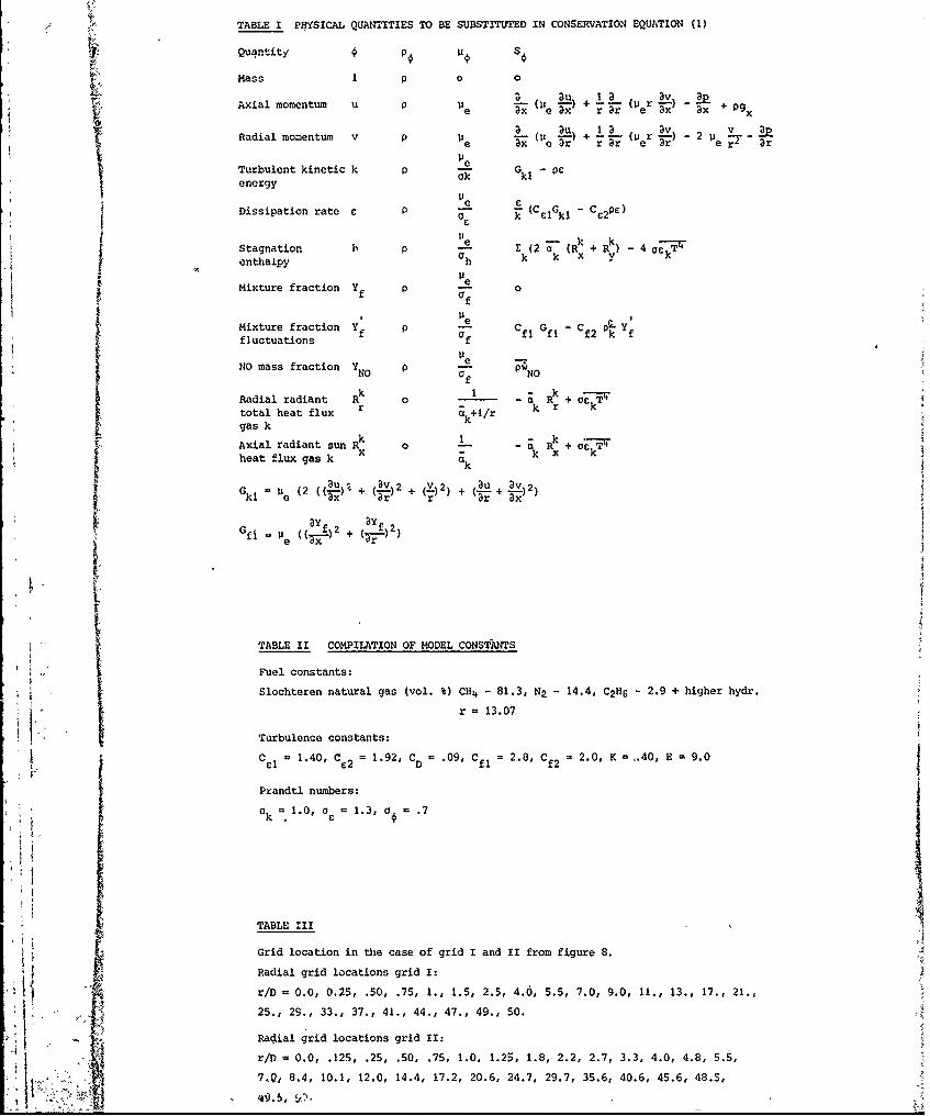
TABLE I PHYSICAL QUANITIES TO BE SUBSTITUTED IN CONSERVATION EQUATION (1)

Quantity P U

Mass P 0 o 0

Axial momentum u P 11eaxau+Pa au T 1 a -r i

Radial momentum v P V Li *(v eu) . ~I (uir~ -v 2 vie ax e a r r etr) er7 ar

Turbulent kinetic k p li Gkl Penergy k1

Dissipation rate C p -C(C Gcc k Ci k1 -cC 2PC)

Stagnation h P E (2 a(Rk +R) 4-40 ,-TVenthalpy Ck x y Ck

of

Mixture fraction YlieG Cfluctuations fOf f fl 2kf

No mass lietonY

Radial radiant Rk o 1 a R k+ ,.T

total heat flux r a Ir k r kgas k

Axial radiant sun R 0 - Rk + -:Theat flux gas ka

a1e xl # r ar ax:;;2 : i :; f2) v +~u+.X2

TABLE II COMPILATION OF MO0DEL CONSTANTS

Fuel constants:

Slochteren natural gas (vol. %)CH4 - 81.3, N2 14.4, CAH 2.9 + higher hydr.r = 13.07

'I Turbulence constants:

C =l , .0 e .2 09, C f1 2.8, c f2 =2.0, K -.40, E =9.0

Prandtl numbers:

0= 1.0,0=F 1.3,0 a .7

TABLE III

Grid location in the case of grid I and II from figure 8.4

Radial grid locations grid I:

r/D =0.0, 0,25, .50, .7 1., 1.5, 2.5, 4.0, 5.5, 7.0, 9.0, 11., 13., 17., 21.,

25., 29., 33., 37., 41., 44., 47., 49., 50.

Radial grid locations grid II:

r/D = 0.0, .125, .25, .50, .75, 1.0, 1.25, 1.8, 2.2, 2.7, 3.3, 4.0, 4.8, 5.5,

7 0, 8.4, 10.1, 12.0, 14.4, 17.2, 20.6, 24.7, 29.7, 35.6, 40.6, 45.6, 48.3,

I I I I I

a. frozen composition (f c.)b partial equilibrium comp. (p e c.)

2000 c. equilibrium composition (e c.)

Natural gas exp aRe =3600. Fr =5125D. a

Do :13,.. D=S.810"3

m

/[

1500 - i

(K)b

1/ c

Soo--500 /

0 0.2 0.14 0.6 0.8 1(fuel)- - - (.Y) (oir)

fig. la. Theoretical temperature as a function of the mixture fraction for different combustion modelsand experimental data obtained in a attached diffusion flame (dashed line3 give the estimatedinfluence of unmixedness).

, . 5 I I I I I

0.20 -

a frozen composition If.c.)

b partial equitlbrijm composition (p.0 C.)c equilibrium composition (ec.)

tlaturol gas exp.

0.15 Re Fr Do 0Cm)

o 3600, 1250. 13., 5.810-3

(rod. prof.)a 3600, 1250,13.4.5,910-3 (ox prof,)'~~ 46 ) 50: 130, 50.20. -3

Yo 9 8500, 70.170.20.10- 3

0.10

xA

ODOX

go b

0 a .A

0 0.2 0.. 0.6 Lis 10

(fu | -0 (I. -Yf) (Ott)

fig. lb. Theoretical oxygen mass fraction as a function of the mixture fraction for different combustionmodels and experimental data obtained in attached diffusion flames (dashed in-tes give theestimated influence of urmixedness). ,'

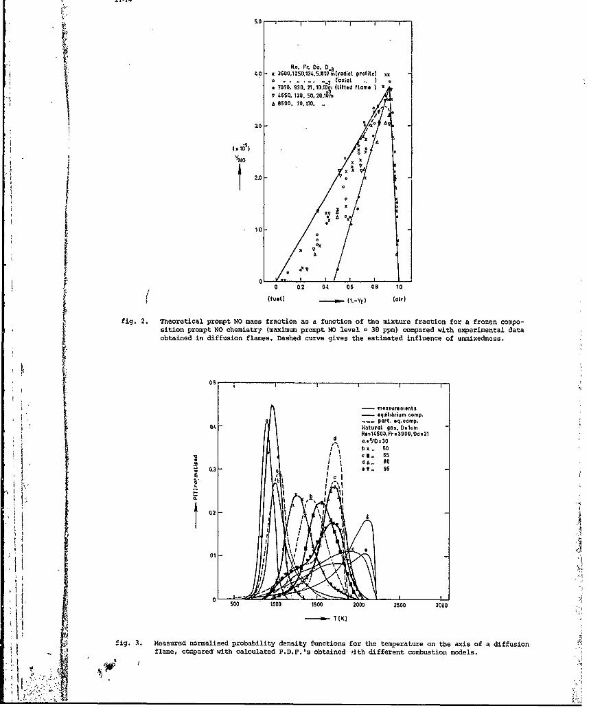
Re. Fr. Do. D~40-x 3600,1250.134,.5.fi10 m(radial profile) xx

a 7070. 930. 21. 10.103T (Lifted flame I x

V 1.650. 130, 50, 20.10ma 8500. 70.170,

0 #'

10

00

0 0.2 01.a 06 8 1

(fuel) - .(l.-Yf) (air)

fig. 2. Theoretical prompt No mass fraction as d function of the mixture fraction for a frozen compo-sition prompt NO chemistry (maximum prompt NO level = 38 ppm) compared with experimental dataobtained in diffusion flames. Dashed curve gives the estimated influence of unmixedness.

- esre et

bb 5

II

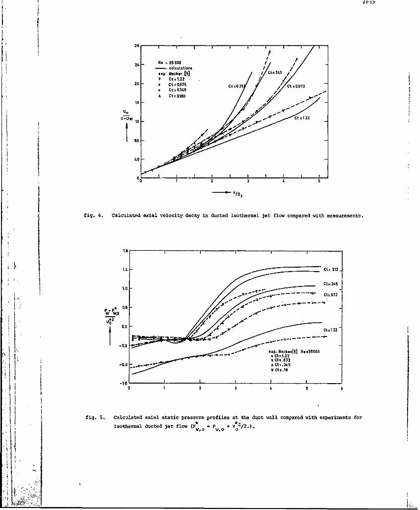
28 ~

24- Re .55000-catcuictions

exp ecker [s] =4V Ct =1.22

20 - X Ct = O675 Q=.021 C ,7o Ct (3.5

I Ct =0.18015

UW12

fig. 4. Calculated axial velocity decay in ducted isothermal jet flow compared with measurements.

1.98

1.4Ct: 2121

Q-045~1.0

*~Ctz,673

0.2

101CW2__ _ _ _ _ _ __ _ _ _ _ _ _ __ _ _ _ _ _ __4_ _ _ _ _ _ __ _ _ _ _ _ _

0xp 1okrS 2 3 5 6

fig.5 * ~lclate axil saticpresur:profle: t te dut wil ~pare witoeCtrial 1.2fo

X Ot .67

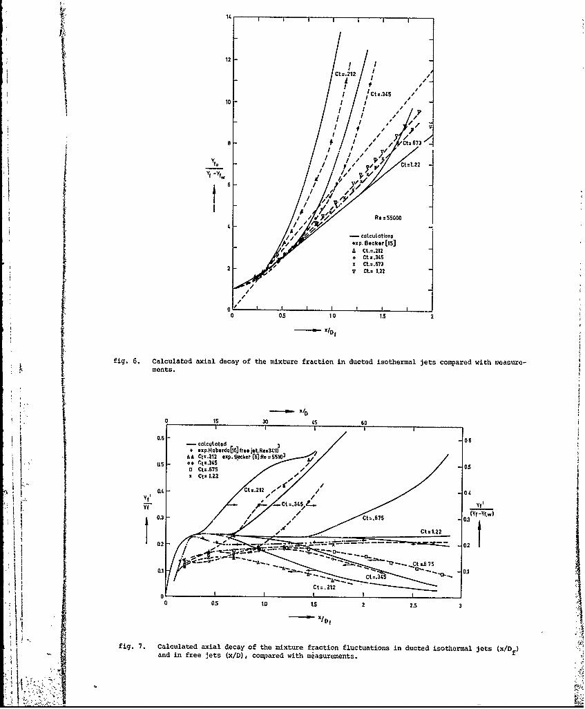
12 Ct=.212

A(

I Ct-3£5 -

xID/

0. - 0 / 6

A//

x tx 1.22y t:2

YfI~ Ctz.21 e/0

0 I ot Ct.345

XV Ct. 1.22

U - 02I

-- A

0 0S .0 i5 605

I I If

0i. .6 06cltdaildcyo h itr rcin lcutosi utdiohra es(an infreejetd 3xDcqae it ~srmns

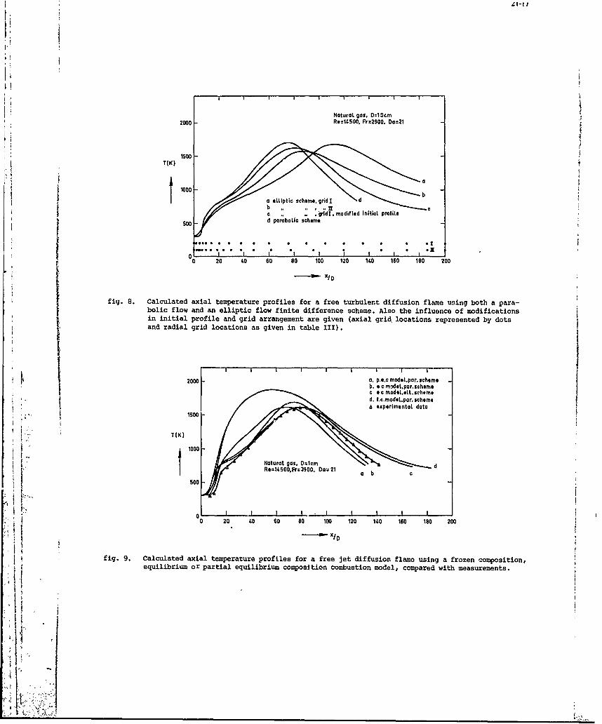
NaturaL gas. 0:13cm2000 Ro=11.500. Fr:-2900. Da=21

1500T(K)

c ., . idI. modifiled Initiat profiteSoo d parabo~ic scheme

I0 0 20 1.0 60 60 100 120 1.0 160 IS0 200

fig. 8. Calculated axial temperature profiles for a free turbulent diffusion flame using both a para-bolic flow and an elliptic flow finite dif ference scheme. Also thle influence of modificationsin initial profile and grid arrangement are given (axial grid locations represented by dotsand radial grid locations as given in table 111).

2000 -a. p.exc modetlpar. schemeb. ee modet.par.schem.sce c moae.tL. che meI. fc.mcdet,par. sch~reeSexperimentaL data

1500

T(1000 -

'c * c.Fr3900.Do, 2

NoturaL gas, DxlIcm d

0 20 1.0 60 s0 100 120 11.0 160 180 200

--- a - XIDfig. 9. Calculated axial temperature profiles for a free jet diffusion flame using a frozen composition,

equilibrium or partial equilibrium composi tion combustion model, compared with measurements.

K U0

Ir -.j7 1.0 elliptic scheme

-porobotic scheme.0 0.8 a Cc. model

b e cmodec' e ecmodel. ignition at xfj :9

0.8 056 Ao experimental data

10 Re :14500. Fr =3900. Do :21

%% 40 60 (t0 100 120 140 160 180

d 20 40 60 s0 100 120 150 160 180X /0

fig. 10. 'Calculated axial velocity and mixture fraction profiles for a free jet diffusion flame. (Thearrow indicates the calculated and measured ignition point).

naturotgos,D.-Icman: gra go0e c 0dit 1

o~R~o~ h. gray/one clear gas... MdeL (Ii]

a oeprana.data

~r(kW/ 2)

at WrD0 50)b

2

0 I 4 0 80 120 160 200

fig. 11. Calculated radial radiation fluxes at r/D = 50, for turbulent diffusion flames and veriouscombustion and radiation models, compared with exparimental data.

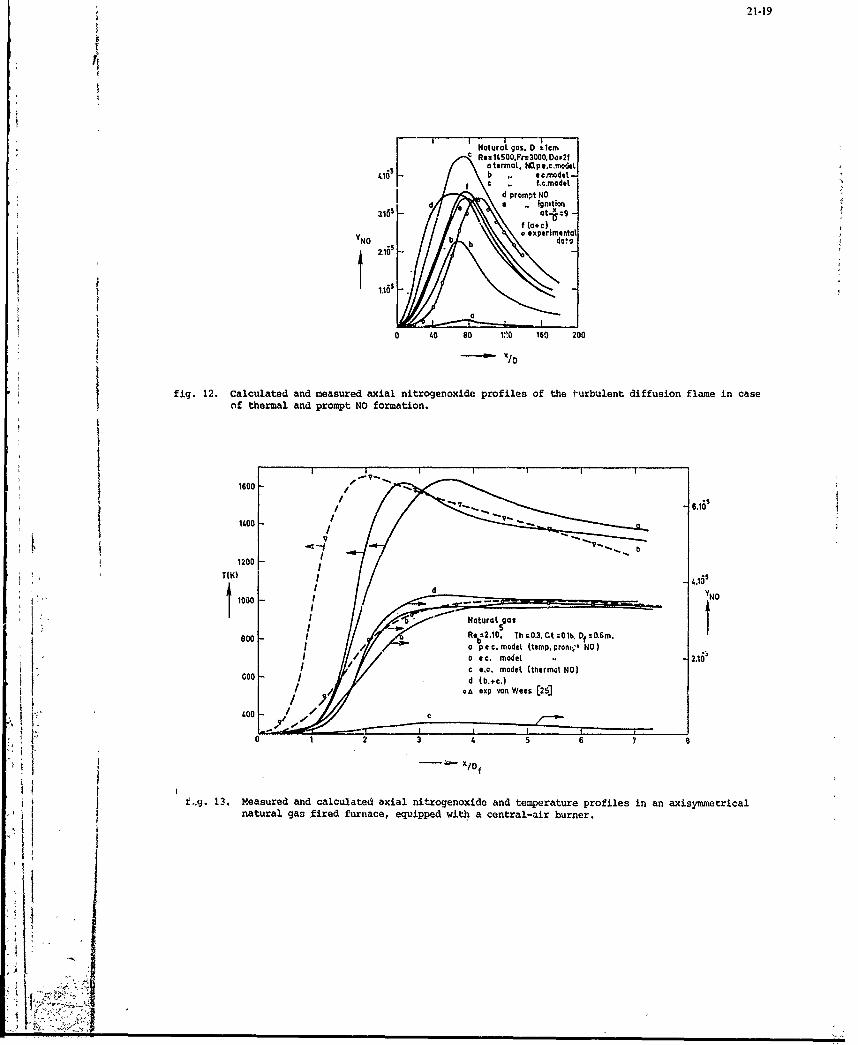
21.19

Natura t gas, D 11cmcRe 1&500.Fr-_300O~a-1I

CterinaL. Npe.c.miuL* cdt4

d d prompt NOd 9 .. ignitior~i

at m~ 19NO experiment:

0 1.0 90 VO~ 186 200

fig. 12. Calculated and measured axial nitrogenoxide profiles of the turbulent diffusion flame in case

oif thermal and prompt No formation.

1600

1 1200 /

T(K

1000 - NO

I NoturaL gas

800 a Re :2.10. Th=:03. Ct :0Th, Of :.6m.

I. e c.mod

GOO - b/.

______________________A________van______________2__]

.yj. 13, lYeasured and calculated~ axial nitrogenoxide and temperature profiles in an axisymmetrical~: natural gas fired furnace, equipped with a central-air burner.

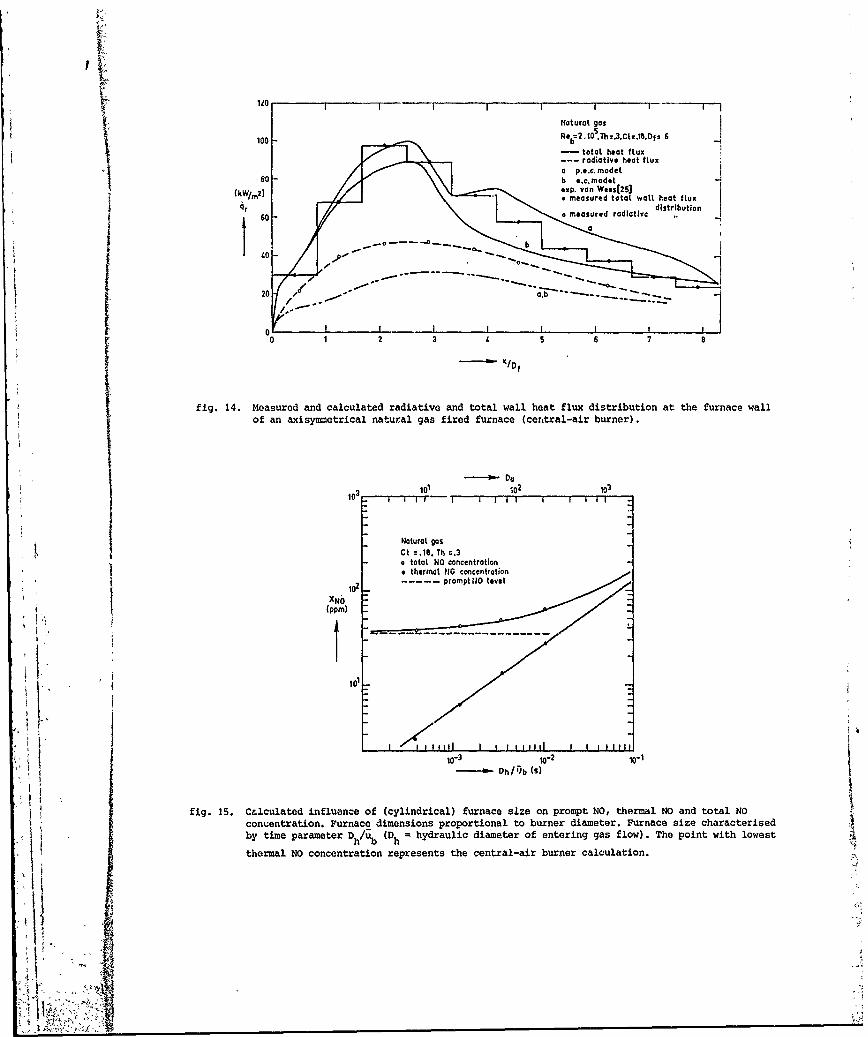
100 NaturoL gas -100 Re:2.10

5.Thz,,3Ct-_.IS.Of-_

80 b P1.lo I(kW/m2) x.vn e[S

I fig. 14. M~~~~~~~~~~~~~ easured n acltdrdaiead total wall heat flux dsrbto ttefraewl

4r 6f an axisasetica nadtutal gat fie fInc (cnra-i burner)

40D

of an axisymmetrical n tural NOs firentuacetionlai ure)

0 totral NOG concentration

102 prompt JO lvet

(ppm)

I il ' 'I : I I I 111 1 11 1

fig. 15. CUlculated influence of (cylindrical) furnace size on prompt NO, thermal NO and total NOconcentration. Furnace dimensions proportional to burner diameter. Furnace size characterised

~fl by time parameter Dh/% (Dh = hydraulic diameter of entering gas flow). The point with lowesth/ I

V thermal No concentration represents the central-air burner calculation.

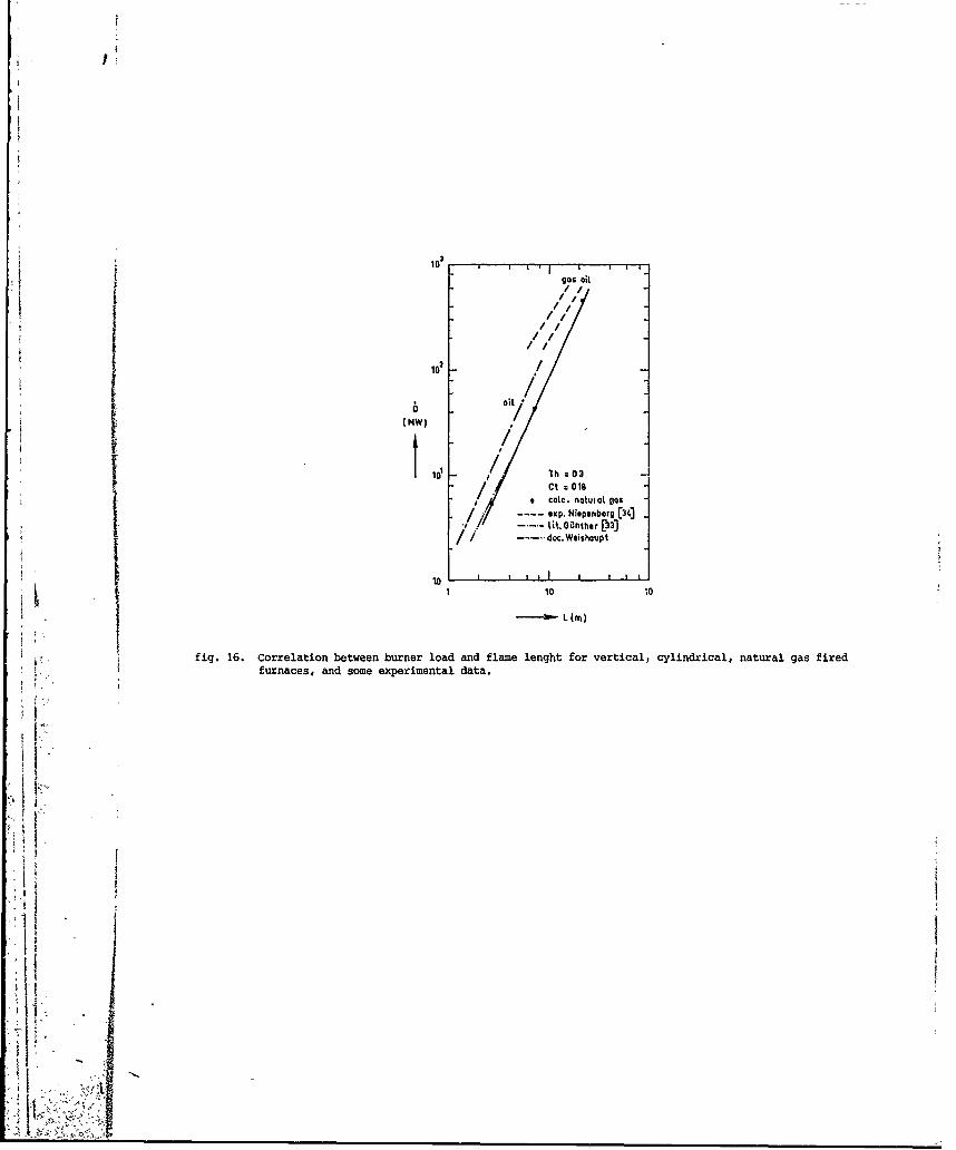
10 !

10gos

'//1

//

102 /

t. ; O~nther [33"]/' --..... doc.W ihoupt '

110 10

(ML W

fig. 16. Correlation between burner load and flame lenght for vertical, cylindrical, natural gas fired

/ - soeepeietauaa

10I

!. 10 10

Ii

21-22

DISCUSSION

H.Eickhoff, GeDid you measure and predict CO-concentrations also? If so, how well do they agree and especially what is yourhighest predicted CO-concentration?

Author's Reply YThe maximum CO mass-fraction predicted with the partial equilibrium composition model is about 3%, a valuethat compares well with the measured maximum CO mass-fractions. CO mass-fractions calculated with the frozencomposition model are very low, while CO mass-fractions calculated with the equilibrium model can reach much toohigh values, up to 10%.

N.Peters, GeLet me first congratulate you for this well documented piece of work. Also I woula like to comment on therelatively large oxygen values that you find on the fuel rich side of the flame. I would think that this is rather dueto turbulence effects than to quenching. In a comment to Janick,'s and Kollmann's paper it was noted that thefuel Aich shift of NO-production could be attributed to turbulence. I believe that a similar reasoning could beapplied to the oxygen shift.

Author's Reply 1In the first instance we have also tried to explain the too high oxygen mass-fractions on the fuel rich side withturbulence smearing out, or better unmixedness. When we take into account turbulent intensities of the mixtirefraction at the fuel rich side, reaching a value of about 45% as calculated with the finite difference technique, wealso obtain much too low values of the oxygen mass-fraction, as depicted in Figure lb by the dashed line above c. 4Also we found high CO and H2 mass-fractions up to respectively 3% and .3% mainly in the fuel rich side, whichindicates that there, incomplete reaction has to take place. The chosen partial equilibrium model predicts wellalso these mass-fractions.

M.N*na, Po ICouk, you give some details on how the calculation scheme accommodates for the height of the lifted 9ame base.

Author's ReplyAs noted in the paper the height of the lifted flame base chosen in Figure 10 is deduced from experiments. Howevera procedure has been worked out and presented beforeI to calculate this height in the calculation scheme. Withthis procedure we were able to reproduce the measured values acturately.

1. Paauw, Th.T.A. Use of the Well Stirred Reactor Concept for the Prediction of Flame Stablization,Bakker, R. 4th Members Conference, IFRF, Paper 15, Noordwykerhout (1976).

TII

tI IL

; , ! o

r[ODELISATICN KkTHEMTIQUE DU FONCTIONNEMENTDES CHAUDIERES DE CHAUFFAGE

EPERTHIJIS, Iigduieur Principal "Techniques d'Apolications Energ~tiques"INSTITUT FRANCAIS DU PETROLE, 1 et 4 avenue de Bois Prdau, 92506 RUEIL MAU4AISON, France

R~sum6

Le mod~le mathdr:tique prdsent6 ici a pour but de ddcrire les PH&-norn~nes rdgissant le fonctiuz'nerjen' d'une chlaudi~re, et d'dtudier leur 6vo-lution en fonction des parambtres pratiltues d'exploitation.

On peut simuler le fonctionneient d'un apparell donnd op~rant enj rdginie continu ou disc(,ntinu.

mances de la c'naudibre,'des param~trcs tels que qualitd du calorifugeage,I fraction de charge, rdglages du brflleur, rdglage du diffdrentiel de l'aquas-

tat.... On peut dgalement prdvoir 1'ordre de grandeur de Is consoarnationd'entretien, caractdristique particulibrement difficile A ddtarminer surplatefirme d'essais.

tia

A

22-2

SYNBOLES GENIERAIJX

A sire-a dpaisseur d'une paroi

CW chaleur sp~cifique du fluide caloporteur

~ 1 EXC (ou eOexcas d'airH coefficient de transferth coefficient d6 convectionk coefficient de conductivit6 thermique

P puissance calorifique au br~leurP puissance utile de la chaudiZreU

Pf pertes par les fum~esP f pertes par les paroiS

p ression0 (ou 6Q) debit calori fiqueT (cu t) tenmpdrature ibsolue (ou Celcius)Ta tempdrature adfabatique de flamme:1 Vd volumeWE, WF masses en eau 6changeur, foyerAll variation dlenthalpieC facteur d.nissif

11 rendementconstante de Stephan-Boltzmann

Inie o regime continud r6gime discontinu (cyclique)F foyerLI f. fumdes ftacudes

22-3

INTRODUCTION

En France, !a consommation des produits p~troiiers destin~s au chauffage domestique et A la pro-duction de i'eau chaude sanitaire eat de i'ordre de 21 MTrEP. C'est un secteur o6 de substantielies dcono-mies d'6neriUe peuvent (1tre obtenues tant par 1'agencement des bfltiments que par le choix judicieux etl'exploitar.ion optimale des g~n~rateurs de chaleur.

La La tr~s grAnde matjorit6 des installations fonctionnent en regime intermittent dit "tout ou rien".Lpuissance nominale de la chaudiZre dtant calcul~e pour r~pondre aux besoins des p~riodes les plus froi-

des, ii en r~sulte que sur une saison de chauffe (correspondant en rnoyenne A 220 jours/an), l'appareilpeut n'avoir fonctionn6 qu'entre 20 et 30 % du temps. Or, pendant lea p~riodes d'arrat, l'eau de chauffa-ge eat maintenue en tempdrature, ce qui provoque des pertes pari , tales rein tivement plus importantes danslea p6riodes de mi-saison que dana lea p~riodes de fort chauffege. 11 en r~sulte que le rendement annueld'exploitation du g~n~rateur sera d'utn neilleur que i'dcart entre sa puissance nominale et lea besoinsthermiques rdels sera faible, et que lea per,,es par lea parois seront r~duites.

Ceci revat une importance particui~re dans le caa des maisons individuelles :dea dtudes entre-prises par lea soct~t~s p~troibres avant la crise de 1973 avaient ddja montr6 que lea chaudi~rea en ser-vice 6taient en g~n~ral tr;-s nettement surpuissantes par rapport aux besoins, et que cette surpuissance

provoquait uxne degradation des rendements d'expioitation.

Pavmi lea formes d'action envisagdea depuis lora, pour promouvoir i'amdlioration des installationsde petite puissance alimentdea au Fuel-Oil Domestique, la profession d~cida entre autres choses d16tudierle fonctionnement des unites de chauffage non plus en regime permanent bien stabiia4 coimne ii eat procddau coura des essaia normalisds, mais dana des conditions aussi voisires que possible de celles effective-ment rencontrdei chez lea usagers.

Dana le cadre de l'Institut Frangais du Pdtrole, une dtude coop~rative coordonnde par l'Union desChambrea Syndicales de 1'Industrie du Pdtroie et regroupant lea principales Socidt~s PA-troli~res, futentrepriac en 1973-74 avec lea objectifa suivants

I/ Etudier sur un certain nombre de pavilions lea besoina rC~els en chauffage et lea consommations.

2/ Procdder A des essais sur plateformes de chaudi~res de petite puissance, reprdsentativea du parcexistant.

3/ ti~gager lea techniques permettant de rdduire lea sur-conaommations engendrdes par le fonctionncment Aicharge partielle.

4/ Etablir un modble mathdmatique cald A~ partir des essais effectuds en laboratoire, et simulant le fonc-tionneinent des chaudi~res. Ce modble devait atre un instrument de travail mis A la disposition des cons-

tructeurs pour leur permcttre une misc au point rapide de leura fabrications, en dliminant un certain nom-bre d'essais longs, fastidieux et ondrcux.

1; Lea rdsultats de cette Etude cospative ont dtd publids par ailleurs [1]. [2].

L'objet de la prdsente communication eat d'exposer lea principes du mod~le mis au point A I.F.P.,et d'iilustrer aon emploi par quciqucs exemples caractdristiqucs.

Rappelons que si de nombreuses 6tudes concernant la mod~lisation des g~ndrateurs de chaleur ontdtd effectudes dana le domaine du chauffage industriel, trb±s peu ont A~td consacrdes au domal.ne du chauffa-ge domestique. Lea quciques travaux disponibles dana la garame des puissances s'6chelonnant entre 15 etquelques centaines de kW, concernent essentiellement l'dtude expdrimentale et la simulation mathdmatiquedes transferts de chalcur dana des chambres de combustion h parois froides pour des fonctionnementa continua

I - PRESENTATION DU MODELE

7 1.1.'Objet du modble et s6tructure d'cnsmble

Le modble a pour but de d~crire lea phdnom~nes r~gissant ' le fonctionnement d'une chaudibre, etd'6tudler leur dvolution en fonction de diffdrents param~tres physiques intdressant la conception et l'ex-plo itation du g~ndrateur teis que :r~glage du brOleur, tat d'isolation des parois externes, r~glage de

Dana la version prdsent~e ici, ce modbic eat destind aux chaudires de chauffage A eau chaudede petite puissance alimentdes au fuel-oil domestique ou au gaz naturel.

11 comprend 4eux parties essentilles, permettant de iimuler respectivement le fonctionnementd'un appareil donnd en regime continu et en r~gime discontinu. Dana son principe, le rnodble eat pr~alable-

ment "cail'sur'un point de foncionniment expdrimentai obtenu au banc d'6sslais ou sur site en regimecontinu. A partir de cc calage initial, on peut alors estimer par le calcul l'influence qu-auront -sur lea

4 ~performances de -la chaudibre- ls qualitd du calorifugeage, la charge, 1'excbs d'air, le r~glage de

P aquastat..

Ecr1tte en FORTRAN IV, is simulation comporte trois programmes distincta nommda CAAGE, CONTIN etSIMULCH. Las deux premiers se rsppor-tent au fonctionnement coniinu, le deinier au fonctiofinement disconti-

nu d'une chaudibre.

1.2. Simulation du fonctionnement continu

I. 2_1 Hypothbsesde base

4La chaudi~re eat sch~matisde sur la figure 1. Elle eat asaimiide A deux 616ments distincta le

rature uniforme caract~ris~e.par TGF darvle foyer kt TGE'dans 1'0hangeur. Ndaninoifis, les temp~ratures de

22-4

Dana le foyer, les transferts entre gaz et parois s'opcrent par rayonnement et convection. S'ii ya un briquetag3, celui-ci eat traitd comine un mur adiabatique retransmettant le rayonnement incident par

7 diffusion-rddmission.

Dana 116changeur, lea transferts thermiques s'opbrent uniqusment par convection. On consid~reque cetdldment se comporte coarse un t6changeur "mdthodique" gaz-eau.

Les Rarois de la chaudi~re se partagent entre surfaces humides et surfaces sbches. Suivant ianature des fluides'prdsents de part et d'autre d'un 6i6ment de paroi, et suivant l'smplacenent de ce der-nier, on distingus les 6 cas ci-apr~s

1 - paioi type gaz-eau 6changeur (GEE)

Parois humides 2 - gaz-eau foyer (GEF)3 - eau-air dchangeur (EAE)4 4- e au-air foyer (EAF)

r4 5 - 0arol yp gaz-air foyer (GA)ao~a ~ch6 - tyegaz-air foyer (GA)

Lea i.rois externes en contact avec i'air ambiant peuvent A-tre ou non murdes d'un calorifugeage.L I

Le~ssur' flux de chaleur DQ eL lea coefficients d'dchange H correspondant A ces situations sont symbo-.lsssrla figure 2.

1.2.2. Transferts thermigus dnalefo

Le foyer eat traitd auivant Ia methode dite du "foyer isotherme", dont la thdorle st due AHOTTEL [5]1.

i a/ Bilan 6ner&6tique du foyer

LA puissance calorifique QF tranamise A la surface de captation A, s'exprime sous deux formes tra-duisant respectivement

leI bilan calorifique des gaz de combustion,

4F - Pi - [AHg T (1)

Lei bilan des tranaferts p~ar rayonnemcnt et convection

C4 - 4 )AQFIG1 TGF 1 T 1(T GF -Ti1 (2)

LP terrme GS1 caractdrise une "aire dquivalente" d'dchanges Oar rayonnement, dont.Ia valeur eatcalcul~e 4i prrtir de dor-ades gdorm~triques propres au foyer (surface de captation A,, surface r~fractaireAr, fnctrur dWangle Frl entre Ar et A1i), des facteurs dmissifs des gaz cg et de la surface de captation Cl.

On a, pour un 1,, A 2 zones de surfaces A1 et A.

1 + iC**l (3)

av~ a-) g.A1 Ar/Ai

La~~ ~~~( fonlta. eoe u sFriJ

L63 effectuds A la FondA Ion de Recherches Internationales, sur lea flammes (FRIF).La llrrmato-, rpoe siriafait qu'on reprisente le facteur dmissif c du milieu gazeux 1"rdel"

cs~ =z 6tanit in scomme p~oddrde des facteurs dmissi fs egnf de n composants gazeux fictifs "gris" rayonnantSsuits '6paiaur cardettristique L. Avec lea auteurs, on adopte ici n -3, et on pose

n:3- c ag,n [I-ekp. (- KnL (4)

Le facteur drn ponddration ag,n ddpend de bn tempdrature effective des gaz foyer TGF par une rela-.~ I [tion de is forms

a-~ b in+ bn TGF

Ua coeificient o'extinctioii Kn 6st la somme des-coefficients relatifa 4 la 8uie et aux "gaz clairs"C32 et 20O. La valeur eat calculable A paitir de la presiii arie du rn~linge (Co2 +~ H20) connue parl'excbs d esi~, del1 conent *a Eion moyenne,e6n par ticu les d6 sit e 'des gaz fo'yer, qu'i I1 faut est imer d'apr bsllexp~ri~fic6-cqtiiie eir 1e' flimfnia de dfffusioi

Toutes ies conitantes ihumdriques perrnsttant d'entrer dana (4) sbnt tlr~es de Ia r~fdrence [6],suivant la- na-ture. id u.:corbuotible'(0 90itit p~trolier liquids ou gaz naturel ric Ihe en mdthane).

-- qui4t& i'paiseur cardctrlitique di rayoniiemeni L, elle eat d~finie dliprbs la relation deHOTTEL VF

L =3, 5 .-I FLa coefficient de ccnvsction hi A -ntrodtuire dana (2) ne peut a'obtenir pratiquenent que par

l'expdrience. En nous basant sur des travaux effectuds antdrieurenent b& l'I.F-.P. aur des foyers e .pdrimen-taux~7joi a u tabi Ia relation emnpirique-.

'h(/ .K) 25,6_ 1 -exp. ( QS/lOOO) ~ (5)

Q8 dtaft une vitease-rndasq~e a didiique (kg/h.M-2) desgaz dana le f6yer.'our 'tenircmp 6orind offcetd 6vcinh avec ls tempdrature, on a utilisd

lstravaux de GiNAPATHYr8 tiiro~td (5) un- terms coriectif tel- que I'expression finale de hi

22-5

devienne TGh=26,41[1 - exp. ( QS/1O00 [1i - exp. ( 2,6. TOF ) (6)

La rdsolution simultande des 6quations (1), (2)Y... (6) permet d'obtenir

Inl puissance calorifique transmise dans le foyer QF, done le rendement de ce dernier9 F F /Pr - les parts respectives du rayonnement et de la convection

- la tempdrature effective des gaz foyer TGF, mais A condition que soit cor'nue la temp~ratureTech des gaz quittant le-foyer.

C'est cette dernibre valeur expdrimentale qu'il faut n~cessairement fournir pour "caler" prdala-

n~anmoins poser A titre d'approximation

blemnt e mo~lemath~maiqu aurl'e ~ech Si laTemG aueTcF' u~temsr npur

A 6tant g4ndralement comprise entre 150 et Tech C A

b/ Evolution du rendement de foyer

En dehors des conditions d'exoloitation de Ia chaudi~re qui ont servi au calage du mcd~le, ileat ndcessaire de savoir estiner les nouvelles performances du foyer.

A cet effet, le calcul du rendement des transferts gaz-piroia 97F en fonction des parambtres de

r~glage du brOleur s'effectue au moyen de In relation de corrdlation de type universel proposde par

Ta -T F7 F~=(

avec I'F - 7 ad 0 (rendement r~duit)

* 3ad (Tad o

.T ad (tempdrature de paroi rdie

A' -~- (Ecart rdcluit des tempdratures des gaz foyer, avec Ia m~me valeur deA que celle du calage).Tad

I La tempdrature adiabatique de combustion Tad se calcule simplement b partir de Il'excb d'air, du

pouvoir calorifique du combustible et de tables enthalpiques sans3 tenir compte des dissociations, ce quiest ici plausible du fait des excA-s d'air pratiquds dana les chaudibres de chauffage domeatique (supdrieursA 15-20 %).A7 est une "aire Equivalente d'ehange", calculable A partir des grandeurs W1 hl et TGF d~fi-nies pr~cddemment

d 1+A11 4 c (TI + TGF)3

En fait, en dehors des conditions de calage du modble (CAL), l'aire dquivalente Anlest pas cal-culde. directeinent, 6t In densitd de feu D' ndcessaiie pour entrer dana (7) eat estim~e d'apr~s la Lelationde proportionnalitd

r ~ r CAL CA3

[D CAL *T -D -A' _FUEL Td] [ad o8IFUELJ ]d-

La temp~rature T, de paroi eat pr~auni~e demeurer constante d'une condition A~ lautre (de l'ordrede 400*K dana une chaudibre A eau chaude).

L'emploi combinE des relations (7) et (8) permet alors d'estimer le rendement rdduit' 9'F pourtoute condition de rdglage du brOleur autre que In condition de rdfdrence -ayait servi'a "caler" le mod~e,

J dlo V'on tire. lea nouvell'es valeura

-du rendement des transferta gaz-paroi Ta

'F Ta T

-de Ia puissance calorifique transmise aux parois

$ F = i - F

-de la temp~raturedes gaz ensortie de foyer Tech telle que

0

-- de la tempdrature effective de foyei

TdF T +ech CAL

Connnissanit QF et TG F, on-se propose. de 6alcul~rhA- la-puissan~e utile trifismise bc iau du foydr PUF,

- lea pertes par les parois-Fhumides DQEAF et celles par lea parois abches DQGAF,- Ia teiapdrature de Il'eau quittant le foyer TEF.

22-6

Cette s~quence du m~d~1e utilise en pirticulier la m6Lhode de calcul pr~conis6: par la NormeBeige NBN 234 [9] pour l'&stimation dui flux die chaletir perdu par un6 paroi externe de Ia chaudi~re connais-sant sa tempdrature auperficielle T~ et La tenipdrature ambiante T0 ..

Lea patois sont assi-mildes A-des zsistances thermiques pures. Pour un -6l6ment de paroi compor-tant n couches de matdriaux setperpos~es (dont 1 dtant le m~tal constitut !), IA rdsistance est 6gale A

aE ni a - tant l'6paisseur et k le coefficient de conductivit6 de la couche de rang n.n k ' a n

n

Lei dquations de base rendeint compte-de la quantit6 de chaleur transmise A l'eau

DQGEF =PUP + DQEAF aeavec PUF = CW. QW(TEF - TO) (9)

-de Ia quan-it.1 de chaleur totale transmise 'dans In~ foyer

QF = DQGEF + DQGAF (10)

A ces dquations sont associ~es des relations faisant intervenir les coefficients de transfert

- entre gaz et paroi interne HGF~1 - entre paroi et aau HEAU (de l'ordr& de 580 W/m2.K)

- entreparoi exterhe et ambiance HA.

On dcrit ainsi

DQGEF , A 1 HGEF . (TGF - TE 4.TEF (1

avec lIW3EF - l/HGF + l/HEAU + a~- (Q 6paisseur de metal c~td foyer)

DQEAF - A1 ECA . TE + TE - T )(12)1 ' HA 2o

avec 1/ECHA INHA + l/HEAU + Ea/k (1 6paisseur de mdtal + couches dventuelles de calorifugeage),

T +QA +T etp1 Al .HA o0

DQEAF -f(Tp 1, To) (13), Ia fonction f r~sultant de 1'emploi de Ia norrne Beige NBN 234 mise sous form'Ianalytique,etc...

La rdsoluLion des dquations (9), (10), (11), (12) .. . par mdthode itdrative permet d'obtenir si-

la tempdrature dleau quittant le foyer IEF.

1.2.3. Tranaferts thermi gues dans1 'dchengeur

etlaL'dchangeur eatsuoposd'ooPer d'une mnanibr6 "midthodique"l entre lea tempdratures de gaz Tech, Tf,

Lea dcarts fie temp~raturea eintre Ileau et lea gaz aux deux extr~mitds sont caract~risds per leurmoyenne logarithmiquo!

(T -TEO r (Ti TS).ech '

1F - TEFlgechloe Tf'-TS,

a/ TrAfiifeit global ettransfert A l'eau,

Le transfert entre lea gaz de combustion et l'ensemble des parois internes de 4i6changeur eat four-ni par le bilan enthalpique

ec= AHJf -DQGEE + DQGAE (14)>11 echQatNla pusac clfiqetass6uxparois humides, elle eat telle que

I - - QGEE k HECH . 8(5

fA 2 dtant l'aire de captat16n et HECH le~coeffi4cient de tranafert, entie gaz et ehu.

b/ Loide vaiiatioiducoefficientd~change gaz-eau

On admet que HECH est -l16 d'une jart iii d6bit masaique Qg des gaz de combustion, et d'autre part A

leui temperature effetive d~finte par I'expressionde

TdE 2 IS-- (16)Pour tenif compte del'dvolutfon due& Q6, on s!edt basd sur. des travaux effectuds A I'IFP sur in gfl-

ndrateuf de I typ Ie commercial [10]. Le 'teimd coirrekif ddOA 1a eaiitureia6t i Ird des travaux de GANAPATHY[8' se raoport i~t~ deas ic6 leienti gazu au 'travis ers -appes de-tubes.

Pour des conditionsdd4 fonctionnemsent hors zde -cell-es, du calage-, on-pose ainsi

22-7

CAL )HA TCQO*0,35HECH =(HECH)CA [;GEALJ()

c/ Bilans thermihiues rqlarifs A 1'eau et aux parois de 1'6changeur

On dcrit un ensemble d'dquations 6nerg~tiques dont la rdsolution par m~thode itdrative permetI d'atteindre:

- lai puissanceutile transmise A l'eau PUECH- les pertes par lea patois humides DQEAE et celles par les parois s~ches DQGAE- la temp~ratuT.e de l'eau en sortie de chaudLie TS- la tempdrature des fum~es 6vacudes Tf.

Aux eixpregsions (14), (15), (16), on adjoint ainsi des relations du type

DGEE = P;'ECH + DQEAE,

avec PUECH =CW .QW (TS - TEF)'

T DQEAE +Toe02 'A' HA'. At

DQEAE =f(Tp 2 ) To), la fonciion f rdsultaint-coime pour le foyer- de l'adaptation~de la Nonme Beige NBN 224.

DQGAE ECHA .A' 2 (TGE -T)

::::il/ECHA = 1/HOE + i/HIA + Ea/k

et 1/HOE =1/HE9CH - 1/HEAJ - a/k

1.2.4. Bilan thermique complet de la-chaudibre

Finalement, pour nn dtat d'isolation donnd de la chaudit~re et pour des conditions d'L,-ploitationI fixdes telles que- debit do combustible QFUEL,- excbs d'air eA,- debit d'oau QW,

f- tempdrature dlntd do l'eau TE,on obtiont pour le fonctionnement continu lea renseignementspratiques suivants

- Ia puissance utile de la chaudite Pu PIIF + PUECH,- le rendement utikI) Ju-P/i

- la teipdature dleau finale TS

- la pte par los fumdes Tf ~Tf- l a ier t pa r des fumtes P7 + lS T'V. - l'analyse-ddtaillde des pertes. pat los patois s~ches et humides.

j:. 1.2.5. Modalit~s prati !quedoa simulation on rdgime continu

LaCNTN simulation du fonctionnement continu fair l'objet do d~.ux progro'mmes distincts nomm~s CALAGE

Leopreiier eat rdserv6 au calagepr~alable Ju mod~le sur un ou plusieurs rdsultats d'expdrienceacquis sun plateforme l dessais ou sui: site . IJn rdsultat d'exp~ience reprdsente une "condition do rdfdren-

jcell caractrnisde~par un r~giage do brCIleur (debit'do fuel et exc~s d'air), une puissance utile do chaudib-to, une'temp~rature d'dvacuation des furn~es et une tempdrature des gaz do combustion a l'entrdo do I'dehan-

geur. epot odto ~~Le second programme exlieun ondto de r ~ence prdalablement trait,,e dans le premier,

avec le doubliojectifII I- de foutrnir une'analyse ddtaill~e du bilan thenmique,dexrapoler les performances du g~ndrateur opdrant sous des conditions diffdI-f.tns de cellos de

1.3. Simul'atian.'du, f6iictiboniimit dis'coninu~i

Les oaltionnrentif~ et sdquence-du mod~le font liobjet du 'programme SIMULCH,Le'oution~imntdiscontinuon~visag6 Ic!. est proyvoqud par 1'aquastat de la c haudiA-re, qui op~re

entre_2 seils de t rtrsdeufixdd par son r~giage diff~rehtiel.

La rrentgd lacaioude e hui or',n"tu ' ie~Pn erd'detpatures dyeP_affich~~~~~~~~~~~~~~~~sW T§ .iejbs oisodn l~eiee ot ub~er t WE. nvauhucrrsodn

Ao paoi &.~chg~ i son assdesA4 &fdes foyate LAErmqepts Masenpini

au~~prL ~ a delul eu~p a longs, on~pout dans -le progl.,3ame pi; ndre en compte lu etetemqeZ4 , ir.4c lc ed erietehrmq ,

22-8

et les traiter conane des murs monodimentionnels.

1.3.2. M~inicion des noefficients dldchange internes

Pour des roisons d'ordre nutifrique, 'on est conduit A exprimer tous les dchanges entre gaz et eaupar des relations lin~aires de la forme

g eauTg s'apparentant b TGF ou A TGE._ _ _

Losu e brflleur eat en fonctionnement, les valeurs des coefficients d'dchange (OF dans le foyer,HECH dar~s l'dchangeur) sont celles calcul~es enr~gime contijnu.

Loraque le br~leur s'arr~te, on a admis pour ces coefficients d'dchange des~ lois de variation ba-sdes sur les considerations suivantes.

VO/ Dans le foyer, apris un court laps de temps, HF s'apparente au coefficient de convection hl et suit Ialoi d'dvolution d6finie par Ia relation t6).

20/ Dans l'6changeur, HECH suit la loi ci'dvolution d~finie par la relation (16).

3*/ La loi de aecroissance du debit gazaux Qg en fonction du tempa eat lin~aire :elle s'~tend ici sur unep~riode de quelques secondes. La limite inf~rieure de Qg constitue le "debit d'air de balayage" provoqu6par le tirage de Ia cheminde. Ce debit l'arrat eat fixd Oar l1expdrience. Des easais effectu~s A IFP ontmontrd que, pour de petites chaudi~res domestiques, il 6tait de V ordre de 10 kg/heure.

enr eAu coura de la mise en route du brOleur, on conserve lea ni~mes lois d'6volution que prdc~demtmentenr edebit de balayage et le ddbit gazeux dtabli.

1.3.. Equations de base

A chaque instant, 1t6tat thermodynamique du syst~me eat caract~ris6 par 6 variables

- 4 variables pour lea gaz TGF, TGE, MF et HE- 2 variables pour l'eau TEF et TEE.

Pour lea gaz, on applique dana le foyer et i'dchangeur lea lois d'6quation d'etat, de conserva-tion de masse et d'dnergie

(p.V)F = F . R . TGF (17)

dt bi fuel + db dair) -di de transfert entre foyer et ..hangeur (18)

d(MF UP) a-d4F +[AH) (19)

UF dtant 1'dnergie interne spdcifique des gaz dans le foyer, et[AH] la diffdrence entre lea ddbits onthal-piques & l'entrde et en sortie de foyer, etc...

an!2Pour l'eau, on applique Ia loi de conservation d'6nergie dana le foyer et l'dchangeur. On dcrit

WF .CW .d(TEF) - DQGEF - DQEAF - (TEF - TE) CW .QW (20)

WE. CW .d(TEE) DEE- DQEAE - (TEE - TEF) CV Q (21)

Le systum d'4quations dtant mis en forme, il reste 6 dquationa diffdrentielles du type

dvi = ~ ... Y . 6

ot) lea yi sent lea 6 variables crtritqe d~ine y6)esu

Connaissant A chaque instant lea valeura de ces variables, leura d~rivdes par rapport au temps ettous lea d6bits-calorifiques mia en jeu, on vdrifie que lea bilana thermiques sont reapectda

F -NICEF + DQGtE - (DQEAF + DQEAE) (22)

P, DQGEF + DQCEE + DQGAF + DG + CHgf(23)

0

13.4. Rernseigettprtqs oni--------------- -,----------------u---o-rns-----a-imult-o

Tous lea debits calorifiques dtant intderds au cours des calculs, onen d~duit lea rendem.nta uti-lea du foar, eldhnere de psc arbi cycle. un cycle de o ctionrement, et leg pertes correapon-

En outre, le~pro ramne calcule pour -un rdgime-cyclique Atabli

la-raciondu emp demaihedu brOleur dana le cycle

PorQbtenir ces-r~iultats A diff~rente cres dg, Is chaudibre, on peut faire varier soit le

debit d'eauQW dans -le gdnirateur, soit Ia tempdrature- A'entf~e d' eau (4ite de retour) TE, soit 46ventuel-lement c' u' aaateapour 'u-r~r l'e-on'f-d aquastai.'

II - EXEMplkS 61APPLICAt1ON DUHMODELE

-j~ ~ ~ ~e exe ealea qui' sivent se-rapportent & deuxc chiudibres -le chauffage dorestquqi n

essaydes-en laboratoire .(parmi, 14autres) ,au cour's de 1'Etude coop~rative-ieni onn~e prdc~deinment [13. [21.Ces deuk appareiLS, repdrdsa. B, et -E. ont une p~ifssneutile no~inale dd l'ordre d6 29 kW~ (25 thlbY.

La chaudi~re B est enacier avec-ballond'e'au sanitaire incorpord. La-,hqudiZre E,. sdns production d'eauchueint~re es-tfnee pour paticulaiii7 d'etr'e tiunie d'ufifo~ferbiqe.

Le combustible =tilisd ici, eat du fuel-oil domestique, distillAt Odirodier -ayant les caractdrisques

22-9

V moyennes sulvantes

C =86 7,H =13,5 7,S =0,5 7.%PCI =42,8 Mi/kg (10 250 kcal/kg). 4

Dans les cas trait~s, Ia puissance appelde (ou charge) est provoqude uniquement par les besoinsen chauffage. Nous allons examiner 1'influence d'un certain nombre de param~tres d'ordre pratique sur leaperformances en nous appuyant sur Ia simulation mathdrmatique, et en comparant dans Ia mesure du possible-es r~sultacs A ceux tirds de 1'exp~rience.

11.1. Influence dii d~bit de fuel

Stir la figure 4 sont reportds les bilans thermiques obtenus en regime continu pour des debits defuel passant de 3,13 Ai 1 ,93 kg/h sur la chaudi~re E.

Au banc d'essais, cette variation de d~bit du brOleur a Atdi obtenue par changements successifs degicleurs. Los per~formances calculdes l'ont 6td A psrtir d'un calage (CAL) dii modZe effectud sur 1'essaiSddbit maximal.

Los rendomients th~oriques apparaissent ici atre quolque peti infdrieurs aux rendements expc~rimentaux, et on voit que les diffdrences sont imputables aux pertes par lea parois. Enl dehors des imperfectionsIinhdrentes A toute simulation mathdmatiqie et auxquelles ce mod~le n'4chappe pas, signalons que sur lesplates-forme d'essais los incertit.des d'apprdciation directe des rendements utiles ant dt chiffrdes auxenvirons de -2.

On remarque imm~diatement quo le rondement utile tend Ai augmenter lorsque le debitde fuel diminue. Bien entendu, ceci eat dO en grande partie A la diminution de chaleur sensible empor-t~e par les fumdes. Mais il faut signaler que le rondoment de foyer lui mame augmente, ccrmme le laisse prd-

voir Ia relation de corrdlation (7) du paragraphe 1.2.2.En effet, on peut montrer quo V' eat une fonction d~croissante de 0'. Loraque dana la chambre

de combustion le rayonnement eat le mode de transfert prdpond~rant (ce qui eat le cas ici o6 le rayonne-ment intervient pour plus de 70 %.), Ia densitd1 de feu rdduitt D' d~croit avec P,, ce qui contribue Aaugmenter le rendement dui g~ndrateur.

L'accroissement dii rendement s'accompagno ici d'uno trbs nette diminution de Ia tempdirature desfutn~es !,.acu~es, commo le montre In figure S. on notera d'ailleurs icJ Ia tr~s bonne concordance existantontre l'expdrience et le calcul.

Cette notion de temporature do fumdes revat tine grande impo-rtance pratique. Enl effot, si tinetempdrature "basse" eat gage de bon rendement, elle petit Ztre dgatement source d'ennuis dui fait des conden-sations poasibles dana le conduit de chemiride quand on attoint le point de rosde acide. Pratiquemont, stirlea installatibiis de chauffage domoatique, on dvito de descondre ati-dossois do 200*C en sorl-ie de chiaudibre.Dana cette opti.que, l'emploi dui modale eat particulibrement efficace pour prtdvoir le ddbit calorifiqueminimal admissible stir tin g~ndrateur donn6. Ceci oat illustrl stir Ia figure 6 :des calculs systdmatiqueseffectuds sur In chaudibre B ant montrd quo, sous pr6texte d'augmenter son rendemont en diminuant an puis-sance nominale (dana le cas d'une surpuissance 6otoire de l'inctallation de chauffage par exomple), onno pourrait songer A descendre ati-dessous d'un r~glage de brOleur corrospondant Ak environ 1,3 kg/h de fuel.

sotiffl6 opdrant ati-dessous de 1,4 kg/h.La figure 7 se rapporte A~ l'6volution du rendement de Ia chatidibre B operant en rdgime discontini

pour 2 rdglages de ddbit du brOleur :3,04 (ddbit nominal) et 2 kg/h (ddbit rdduit). On constate quo IAencore, pour tine puissance appelde Pu ou fraction de charge ot donnde, le rondement augmente quand onKi: rtdduit le ddbit do fuel ati-brOleur.

Le calcul parait ici devoir surestimer lea rendements exptdrimentaux :mais il faut save'r qulaucours do tels eesais, il eat difficile do maintenir constants lea parambtres do rdglage dti brleir (ddbitdo ;ombuistible et excbs d'air), et Ia temprature moyenne do l'eau.

L'alluro do ces courbes do rendement eat tout-h-fait caractdristiqie de cello rendant compte desperformances d'une chaudi~re fonctionnant en regime "tout ot ien". On notera que In d~croissance du ron-dement eat par'ictilibroment. 6Arqude h faible charge, ati-dessotia do 25-30 '.pour cetto haudire. L~e detaildojs pertes eat fourni aur Ia figure 8. On remarquera quo los pertos par lea patois, qui varient assez peien valeur absoltie -ave-. Ia puissance appelde Pu prennent do cc fait tine importance relative croissante quand1-lachArge do Ia chaudibre diminuo. D'ob lintdrat de choisir tin gdnt~ateur dont Ia puissance maximale nosalt pas exag~rdment au-delb des besoins thermiquos rdels, sous pr~texte do so manager tine rdserve de

j ~ puisa-ance,I. Actuollement, pour tenir compte des becoins inat~antan~s d'eau chaude sanitaire en masison mndivi-

j duelle, on prdconise d'opter pour tine puissance install~e sup~rieiro d'environ 30 7. 4 lua puissance dochauffage n~cessaire par grand froid.

conommtio decombtistible,,din-gnraetirde~chaleur.La igue 9monre e gindo rendernent qu'on serait susceptible d'obtenir sur Ia chaudibre B (en

foncionnmcin. cotinu en' ~ d6un ekct-kd''-s d'ai do 60% A tin exc? s d'air de 10 7.: gain d'environ I

Lem~eOre 'xlctrici lspdone ieneuOnotenfe faire ermaqs

In ilsor i'ndmetal 'e, ~taccroissement do rendement oa e uinain eI eprtr daaiudcombusat ion 'Td u contiibie diminuer Is densft6 4e feui r~duite D1, donc A accroitre le rendemento dlonnc& pa'r Ia relation do corrdlation (0).

"t, V/ Par contre, le rendement de 114khangeur crott avec I'exc~s dWallr ceci oat dO A l'amdliorltion ducoefficient'do transfert, cons~cutive A tine augmentation du ddbit ma-saique des gaz,(kelation (16) dii Para-~ bie quo eur-tempirature tec diminue.

3/Finaleimet, dii fait de Ia partprdpond~rante prise par le foyer clans lo b1ilan thermique. do Ta chaudire,cs Si accroisseme'ht de" iondement a~'ec ii diminution de, i'e*'cts d'air qui conditionne celui do ['appareil.

R~appelons quo anor les chaudibres de chauffage aomeacique pavillonnaires qtii sont d~munies par

22-10

principe de syst~mes de regulation sophistiqu~s, on ki~te g4n~ralement de r~gler le brOleur au-dessous de20 7. d'exc~s d'air, ceci afin de se m~nagez une marge dei s~orit6 quant A Ia qualitd de la combustion.

11.3. Influence de la tempdrature de i*eau

Un moyen pr~conis6 pour am~liorer le rendement d'exploitation, est Je r~duire In temp6rature de1'eau de chauffage.

Prle calcul, nous avons abais6de 20'Cla temprature de 'eau circulant dans laachaudiere E.

peret 'acrotred'ne anbrenotbl teredemnt tie. arexeple pur necharge de 30 %,celui-ci passe de 75 & 78 %., soit uile reduction de consommiation en fuel de l'ordre de 4 .

En dehors des probl~mes propres ? ladaptation des dmetteurs (radiateurs) aux "basses" tempi~ratu-res du fluide caloporteur, I'abaissement de Ia tempdrature a de toute mani~re une linite :le retour del'eau A Ia chaudi~re doit,dans toutc Ia mesure du possible, demeurer sup~rieur au point de rosde humide desgaz de combustion (de 1'ordre de W5C avec le fuel envisagd ici).

Ei ce qul concerne 1'emploi du inod~le, on notera stir la figure 10 la tr~s bonne concordance exis-tant entre' points calcul~s et points expdrimentaux. 11 faut souligner que dans le cas envisagd ici, lesconditions opdratoires au banc d'essais s'6taient maintenues particull~rement constantes et proches desconditions de calcul.

11.4. Influence du diffrentiel de l'aguastat

L'influence'6ventuelle du diffdrentiel de l'aquastat dquipant Ia chaudi~re est particulibrementdifficile A mettre expdrimentalement en dvidence :des fluctuations extdrieures incontr6lables, suscepti-bles d'atre rencontrdes sur un-banc d'essais, peuvent en effet masquer un phfnom~ne aux proportions

mdse.Par le calcul, nous avons envisagd trois cas pratiques correspondant A des diffdrentiels respec-tivement dgaux A 8, 5 et 30. On a simuld le fonctionnement de is chAudi~re B opdrant A environ 1/4 de saj puissance nominale. Les principaux r~sultats de-calcul sont regroupds datic le tableau ci-dessous.

FONCTIONNENENT DISCONTINU

Chaudibre B e a 3 5 %* - QFGD 3,04 kg/h - tE -600C

Rdglage Durde d'un cy le (a) Consom. Energie Pertes ph-_ Pertes9fuAquastat -marche arr~t totale FOD (kg/h) utile (wh) rois (kWh) mdes (kWh) u(%

_________ bra leur brOleur _____ _____ ____ __________ ____

72-80 i75 461 636 0,832 7,44 0,81 1,73 74,875-80 134 344 478 0,85) 7,57 0,82 1,76 74,8

L_77-80 97 254 351 10,841 1 7,47 1 0,82 1 1,74 1 74,7

lNota .Lea bilans thermiques sont iapportds 4 h de fonctionnement cyclique..

On ne peu. distinguer de diffdronces bien sl~ttificatives entre lea performances, malgrt, lea durdesde cycles diff~rant senaiblement'd'un rdglage A l'aurre (vorrespondant b 6 allumages/heure dans le ler caset 10 dans le 36). Tout cu plus peut-on rernarquer que le niveau moyen de ternpdrature d'eau ten~d b augmenterquand le diffdrentie1 diminue,,et qu'on peut slattendre de ce fait- A uvt accroisseaeik des pertes paridtales.Mais ce dernier phdnombne ne pourrait vraiment Otre sensible qua sur des chaudi~res mal calorifugdes.

Pratiquentent, le diffdrentiel des aquastats dquipant les chaudibres de chauffaga domestique sesitue entre 5 et 10*C.

11.5. Influence du calorifugeage

Le calorifugeage eat une caradtdristique d'dquipernent ayant une grande importance sur Is rendepett d'exploitation du gdndiatedr.

Par le modbla, nous avons 6tudid Ilintfloence de 116tat dlslto en fonctionnement continu pourdiff6rents ddbitbs de fuel, en opdrant 6ur Ia chaudibie B (bien reprdsentative en 1977 de Is qualit6 couran-Le d'isolation renontrde sur ce type d'appareil).

On a c6ni~idr 3 dtats d'isolation difftlrents :le calorifugeage d'oiigine, l'abaence totale decalorifugeage, et un "super calorifugeage"l consistant en 1'adjonction A l'dquipement commercial d'unecouche suppldmentair6 di 0i mm de lain6 de verre our toutes les surfaces.

11.5.1. Influence sur le-rendement

L'examen da is figure 12--permet de faire deux constatations essentielles.

10/ Un calorifujeage tr?-s poissd permet d'escompter des gains sansibles par rapport aux performances ini-tiales 3 points do rendersent Jusque'vers 2,4 kg/h, 4 points au debit de 1,4 kg/h.

2*! La variAtion du rendement avec le d~bit de fuel eat d'autant moins sensible que Ila :haudike est momnsI ~bion calo ,rifugoe.

11.5.2. Analyse ddt~illia des -per tes _ea lea _Esrdfs

iI L'analyse d~ta-illde des partes par les parois, rendue possible par Is simulation math~matique,,m6a ate i'vidence lbsr r8les respecif jdu~s par lea Isurka~ei humides e s%,ches dans le bilan

'Ajde6 perteis; Sui la-chAudfbr BenvisagEdWfc[_i, las surf -aces s~chei 'isnes 1%d ssraettlen cdntact i'vec l'ambiance. prstet17.dlaufceoae

Sdzr la figure 13, on peut faire les observaidofis suivantes.V/1' lai pertes fotales par les parois scnt fortement influenceis pai lIEGat d'±aolition, ee elles croissentd 'utant pls -vite savec Lahar'e (celle-ci dtant'ici con'~on~ pa44dbi efel e caoiu

'A ~geage eat moins sAgn6.2 -/ Pour un caloftfugeage 4o~n6, Is *loi- de variation des pertes auk~ parois est essentiellement r~gie parcella des paioii s0ches.- 'ls ertgi par lea parois, humidei vaxiant Eirg peu. 'Cecli eat 'dd au -fait que lors-qua la-cha ge croit en r~gime onnu lenve~u moyen des tempiliatures internes.des gaz augmente, d'o4

22-11

une 6l6vation de temp~rature des parois non irrigu~es par l'eau.

301 Les~pertes totales aux patois ne peuvent atre considdr~es conmne 6tant pratiquement constantes avec Incharge que dans le cas du calorifuget.ge trZs pouss6E, qui att~nue fortement Ileffet dG aux patois sechas.

111.5.3. Influence Sur la temp~rature et les etsp esfms

V La figure 14 montre que l'salioration du calorifugeage est susceptible de provoquer une augmen-tatioi dE'.elable de la temp~rature des fum~es (donc les pertes par chaleur sensible), bien qje le rendementde !a<chaudi~re augmente.

Ce paradoxe apparent, confirm6 par l'exp~rience, trouve son explication dans l'analy-,e des ph~no-mbnes t.hermiques internes A la chaudiZre. Le calcul montre en effet qu'une forte diminution des pertes parlea parois impiime auxgaz de combustion un surcroit d'enthalpie qui ne se tranamet pas int~gralement aiI'eau, du fait des limitations dues aux coefficients d'dchange.

11.6. Calcul de Is consommation d'entretien

Si on rapporte lea pertes totales (fum~es + parois) exprimdes en valeur absolue A la charge appe-M~e (ou puisaance utile 6quivslente) en fonctionnement discontinu, on trouve une relation pratiquement linE-ai.re illustr~e sur les figures 15 et 16 pour les chaudi~res B et E.

Cett: propriftd de lin~aritd, largement confirmde par l'expdrience [1], [2], provient du fait que

-lapertes par lea patois humides sont pratiquement constantcs,- lea pertes par lea patois s~ches et par les fum~es sont sensiblement proportionnelles au temps

de marche du brOleur.

Lorsque In demande en chauffage devient nulle (V u 0), Ia chaudibre fo-ictionne en rdgime ditd' entretien" :le brOleur ne se met en route que pour maintenir l'eau A~ Ia temp~rature de consigne de

l'aquastst. La consommatio. de fuel correspondante Co, qui ne sert qu'At compenser les pertes de I'appsreil,eat une notion intdressante A connaitre :elle permet de juger de la qualitE du gdn~rateur, et en psrticu-lier de celo do son calorifugeage. La mesure pr~vue dans la nouvelle normo frangaise d'essais do chauditre[11], eat tr~s ddlicate. On doit rechorcher un rt~glage d'aquastat permettant de maintenir A une valour im-posde Il'cart entre la temp~rature moyenne do l'eau de In chauditre et In tempdrature ambiante (cet dcart

j eat de l'ordre de 500 dans Is norme prdcitde). Pour obtenir uno pr~cision suffisante dans In mosure des

f2 consommations, l'ossai sur plate-forme doit so ddrouler sur une pdriode proche de 2'4h, et durant cette pd-t rnode la collule d'casais doit Utre maintenuc ? une temp~rature auasi conatante quo possible.

Ld modble pormet d'estimor h priori Is consommation d'entretion.En se reportant A la figure 3, on voit que le rdgiiaz d'entretieu correspond ZI une circulation

d'eau chaude s'dtablissant d'une manibre naturelle (par thermo-siphon) dasla chaudibre, Ia vanno 3 voiesdtant compl~tement ferm~e du cbtd circuit do chauffage. On entre dans le modble mathdmntique en posant quece d~bit d'esu eat trba faible (on a pris dana lea exemplos citds 1 % du d~bit nominal), et on prend pourtemp~rature do rotour TE cello correspondant A la plage infdrieure de l'aquaatat (consigno TSI).

On donne ci-dessous lea r~suitats obtonus A partir des chaudibres B et E.

Rdgime d'ontrotien - Calculs effectuds avec un ddblt d'eau interne di 10 kg/h

Lhudb RE lage brOleur Rdglge sQuas1tat tar Dur~e du cycle (s) CI ______ ~TSl TS2 A A a marche art oale

ha3s13 25 85 j90 20 66 26 700 [ 726 (0,114

L'Ecart Aesu correspond A In oiffdrence tm - C ve + TS2\-TEau5 A ite tm( l 2, -E

Les consommations dlentretien reportdes ci-deasus correspondent A des pertes reapectivement Egales4:1,03 kWh (882 kcal/h) pour la chaudi~re B et 1,31 kWh (1125 kcal/h) pour Ia chaudire E.

En se reportant aux figures 15 et 16, on remarque que cos per tea au voisinage do In puissance

nulle sont sup~rieures A cellos qu'on obtiendrait en prolongeant lea droitea au-delh du point a. Celas'explique par le fait qu'en rdgime d'auto-entretien, pour un r~glage donn4 de l'aquastat, In tempdraturemoyenne de l'eau eat prise sup~rieure A celle du fonctionnement normal :ainsi par exemple pour Ia chau-f dibre B, t 68,8*C en fonctionnement normal (avec tE = 60'C) contre tm = 76,3*C en r~gime d'entretien

puissance nulle a dtE particulibr-ement bien mise en Evidence, sur le plan exp~riraental, par SCHLIENGERet THENARD [12). Pour parvenir A t'ordonn~e d'origine de la droite, lea auteuija pr~coniaent d'effectuer

l'essai d'suto-entretion "avec une consign6 d'aquastat correspondb.nt aux environs des 2/3 de l'Ecart detempdrature entro In consigne d'aquastst de is chaudibre en marcho continue et In tempdrature ambiante".

La d~finition pr~cise de la droite Etant sinai obtenue par deux points correspondant d'unepart au r~gime nominal et d'autre part all r~gime d'entretien reajustE, on peut slots expliciter le rende-II meat de chhudire par une expression pratique do la forme

I' 9 d 9 c (1 -- . c) (24)

m Etant le taux do marche du brOleur, et c un coefficient d'entrvtien thermique ddfini par I'expressionC0

Q FOD

CONCLUSIONS

Un modble mathdmatique a dtd crE4 bt i'Institut Franqais du P~trole, dana le cadre d'une Etudecoop~rative men~e aur lea potites clhaudibres de chauffaga. dorestique.

Pour I'Ecablir, on s'est appuyE aur les r~sultats exp~rimentaux obtenus sur plates-formes d'essais.J Ce mod~Le n'est pa5-un mod~le de conception, mais un mod~e d'exploitation. 11 petmet d'Etudier

22-12

le comportement d'un g~ndrateur donnd sous l'influence de divers param~tres tels que :r~glage du brflleur(ddbit de fuel et exc~s d'air), C~ta-, d'isolation des parois, r~glage de l'aquastat, et ceci A partir derenseignements fournis par 'an essai effectud en regime continu, ou tirds dventuellement du catalogue cons-tructeur. En particulier, on peut suivre d'une manibre plus d~taill~e et plus fine que par 1'exp~rienc-la repartition de 1'6nergie introduite entre 6nergie utile et pertes, et en tirer les consequences pourar~idliorer les conditions d'exrloitation ou orienter une nouvelle conception.

t La simulation du fonctionnement continu peut s'effectuer ind~pendemment de celle du fonctionnementI discontinu, le modle ayant 6it6 prd-alablement cald sur un rdsultat expdrimental.

es Cette possibilit6 permet ainsi d'explorer rapidement l'influence d'un ou plusieurs parambtres surlsperformances en regime continu, et de r~server la simulation du regime discontinu -beaucoup plus longue

en temps calcul- A ''tude de conditions s~lectionndes.Dans le cadre de l'IFP, un emploi caract~ristique de ce mod~le concerne actuellement 1'6l'3boration

d'un ensemble de donndes reliant la consommation a la puissance utile pour difffrentes conditions externes,ces donn~es devant atre utilisdes ensuite dans un mod~le de b~timent rendant compte du bilan 6nerg~tiqueannuel.

On envisage 6galement, sur la base d'expdrimenLatiorS nouvelles, l'extension du mod~le aux chau-di~res de plus fortes cepacit~s que celles considdr~es ici :quelques centaines de kW, domaine du chauffagecollectzif ou industriel. L'un des objectifs de cette extension est 1'dtude fine des avantages respeclzifsdes marches tout ou rien et modulante.

'A V1

.z. 22-13

BIBLL)CRAPHIE

[] S. GAUFFIER, F. MAUSS, E. PERTHUIS et J.P. SCHLIENGER

"Journde d'6tude sur 1'utilisation rationnelle du p~trole pour le chauffage",

Table ronde N' 3 (Rendement A charge variable des petites chaudires). A.F.T.P. Paris d~cembre 1976

[2] Idem. A.I.C.V.F., Paris, avril 1977

[3] .PeLE BRETONde cecsUiest oefvir17

"Transfert de chaleur dans les foyers induatriels"

[4] P. ANGLESIO"Attuali possibilita di valutazione dello scambio termico in focolai di caldaie per ricaldamento"I Atti E Rassegna Tecnica Societa ingegneri e arc~hitetti in Torino. N. Serie A 32, N* 5-8, Maggio-Agos-I

to 1978, p. 109-115

[5] H.C. HOTTEL, A.F. SAROFIM'"Radiative Transfer"

Mac Graw - Hill Book Company, New York 1967, chapter 7-8

[6] T.R.,JOHNSON, J.11. BEERii "4th Symposium or' Flames and- Industry"

Paper N*4 (zone method analysis of radiant heat transfer a model for luminous radiation). TheInstitute of Fuel, London 1972

[7] F. MAUSS, E. PERTHUIS

"Transferts thermiques sur foyers exp~rimentaux".L RovuL Institut Frangais du P~trele, vol. XXV - Nol, 1970, p. 56-88

"Quick Estimation of Gai heat'Transfer Coefficients".Chemical Engineering, September 13, 1976, p. -199-202

[9] INSTITUT BEWE DE NORMALISATION"Mdthode d'essai des chaudibres de chauffage central".

NBN 234, Bruxelles i957

[10] F. MAUSS, E. PERTHIJIS"Transierts thermiques dans Jes chaudtt.es A eau chaude".

Revue Inptitut Frangais du Pdtrole, Vol X)JI1, N' 7-8, 1968, p. 988-1022

[11] ASSOCIATION FRANCAISE DE NORMALISATION"Chaudibres automatiques fonctionnant aux combustibles liquides, dquip~es de braleursA pulvdrisation"

Projet AFNOR E 31-353, Paris 1976

[12] .1.P.SHLIENGER, P. THENARD"Rendement moyen d'une chaudibre de chauffage domestique"

Doc. SHELL FRANCAISE, (rCAR PTh/EB N* 13/79, Centre de Recherches de Grand-Couronne, mars 1979

i 4_J1 P

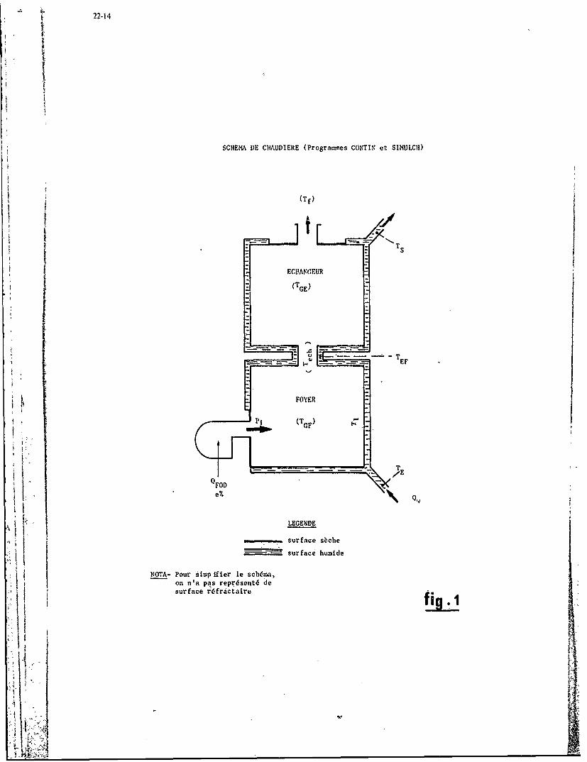
22-14

SCHEMA DE CHAUDIERE (Programmes CONTIN et SIMULCH)

(Tf)

Ts

ECI!AN(.EUR

FOYER

A .A

LEGENDE

surface sbche

Ssurface hurnide

VOTA- Pour simp ifier le schdma,on n 'a pas reprdsentd de

A surface i~fractaire

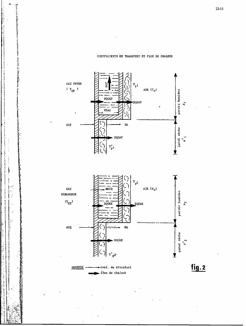
22-15

COEFFICIENTS DE TRANSFERT ET FLUX DE CHALEUR

GAZ FOYER()

)F AIR (6

!q Dwo DQE.AF,

0.

HGF -HA

TpI

V~ 2)GAZ "HECH AIR *T,

ECHANGEUR- -

(TE GEDQGEE DQEAE

) 0

AGE-

.0

i I LEGENDE -. coef. de transfef fg.Holo -ux de chaleur

22-16

LU

00

LU

toU

Im=

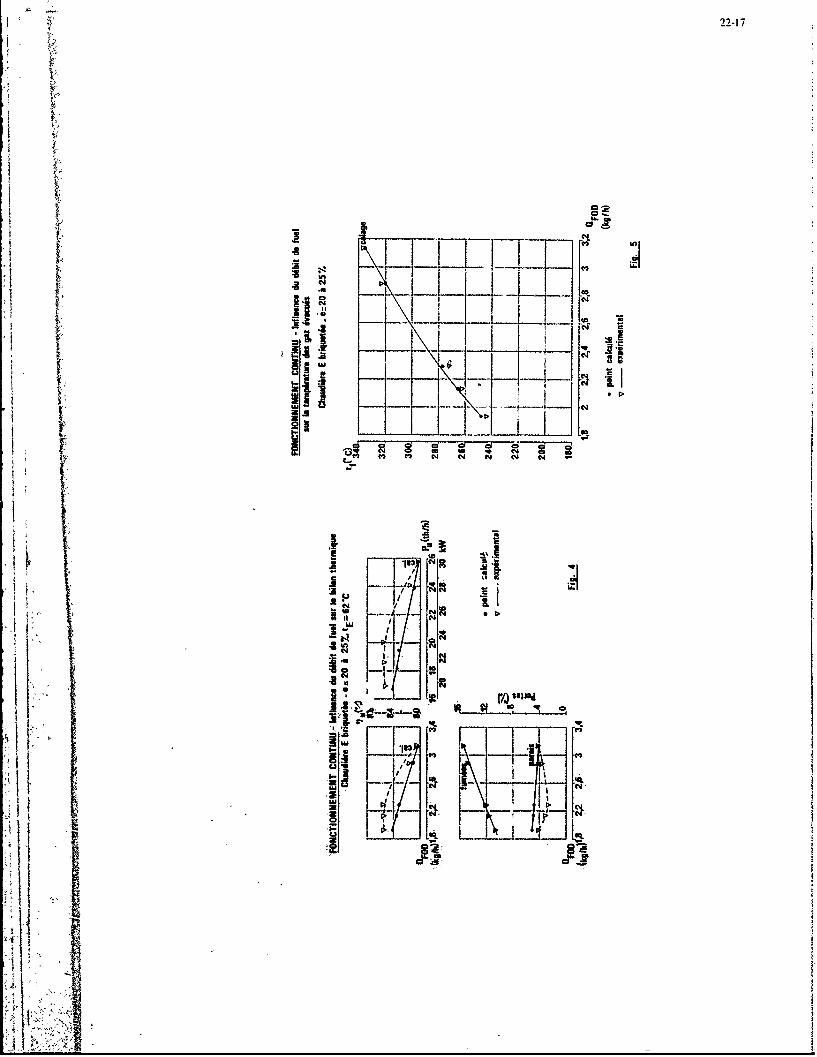
22-17

- - _

i .......... ..-I l

$sli

41,.-'--t'C4,

oi.1

K tP // II

1w]

22-18

__2 -_ ft_-

CD

LUU

C',O

45F ___ N

-m Im

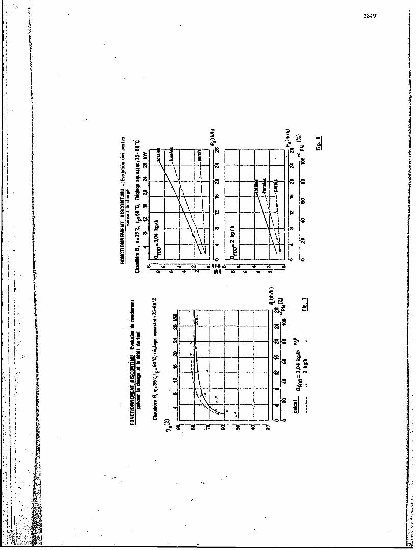
22-19'

A V IL

ca N

- 0 a

II

e- Iin 5

o Go

L6 ~ - -~- -.___ __ __

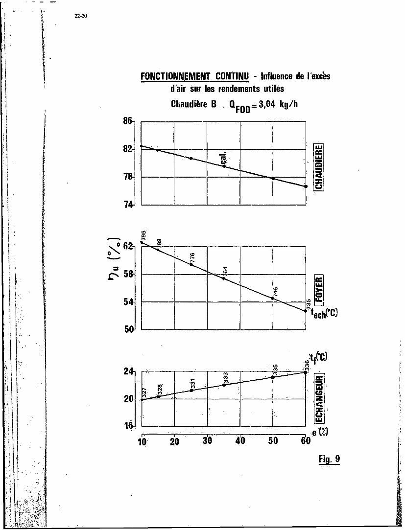
22-20

I FONCTIONNEMENT CONTINU -Influence de Iexchsd'air sur les rendements utilesCIhaudibre B (1 F0 3 ,04 kg/h

86

~LL

062-

58IsU

50

AatftC)

20 2 0 4 0 6

Fig.16J10 0'0 A 0

22-21

110

,CI I--N

E s us

CIO

, ' .... .. I - 0,, -I .

41,

to

VA,

U Cd

l6I = . 0

-up 'r- t

22-22

FONCTIOfdNEMENT CONTIND - Influence dhu calorifue stirIen panies aux paris

Mauike 8.e351%. :57C kW

24 3kh FONCTIONNEMENT CONT114U - Influence du culorifugeags stirhumidei 34 Ii tempilaturs dns gaz dvacu~s

Chaudlire B - e 357.FOD 3,04 kglh

il- -- - -tfeC) 38 -

340_

-1,2 300

2,2 220

1,8 212 a~ 0FOO (kg/l)

bA -. calorifugog normal

_ ~ super calorifugleage0 12 11618 202Ili--snfg U i6 ~b 2t i 2 8 30W

Fla. 13FI.1

FONCTIONNEMENT CONTINU - Influence dhu calorifugagp tir We rendeeet util

Xhuudiee '1 a. 35.tE%57*C

9 14 -16 1.8 20 22_24 26 2i 30 kW

~114 "~ 7iilzi

calo noralFg 2 Ihh

supe bawl'paVe

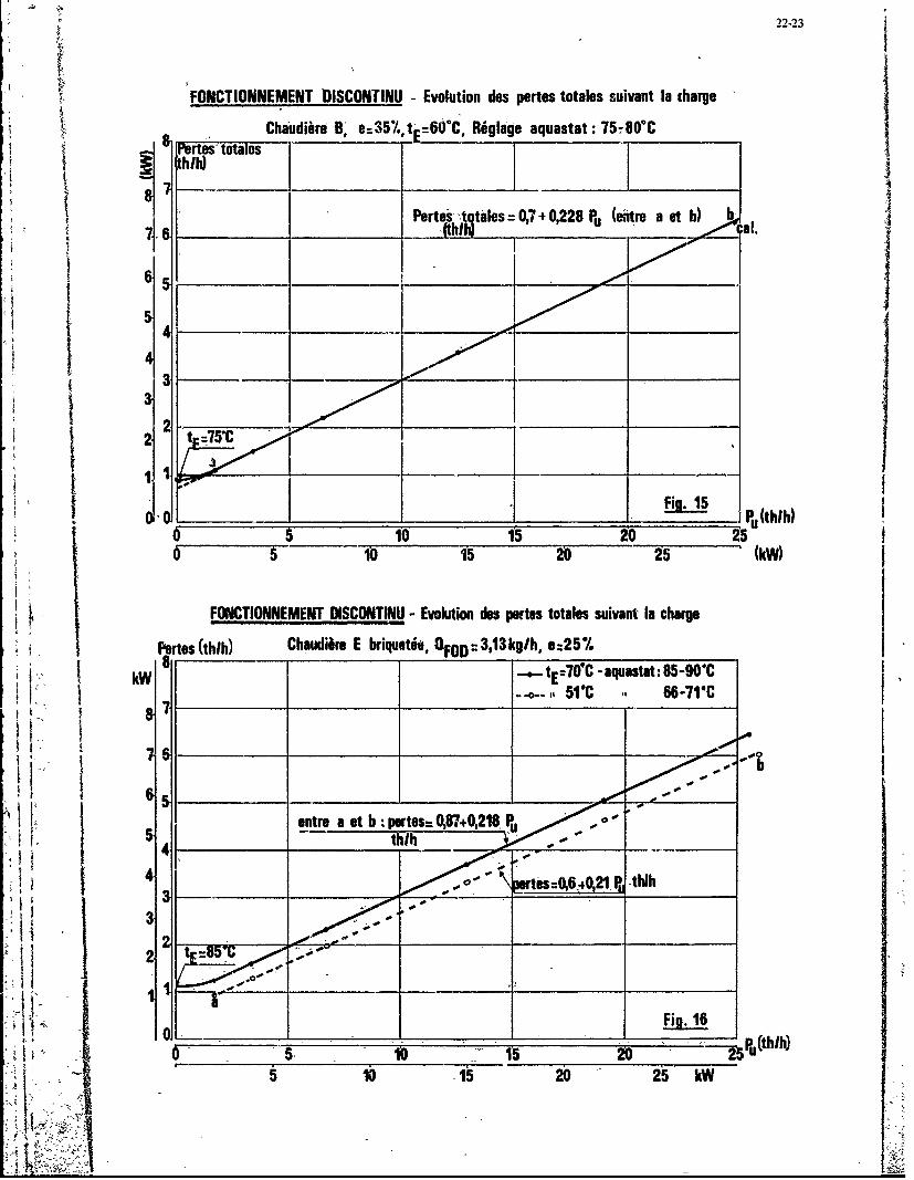
22-23

FONCTIONNEMENT DISCONTINIJ Evolution des pertes totales suivant la charge

IChatotawes e=3 5* t,=00C, ige aquastat : ___________

Pertestqtales =0,7-+0,228 Pu (ehtme a St b)(tli ____________ t

I __ __ __4

3 ____

ib IFig. 1515P 1(thih)

661Is20 -2550 Is5 25 IMW

FOtJCTIONNEMEMT ISCONTINU - Evolution des pertes totales suivant la charge

~ WPertes (thlh) Chaudire E briquotdo, 10100::3,13kg/h, e--25%.

kW -E = . 70C -aqustat: 85-90T

IL. , ________ _________ --- ~B5VC U.6-71C

entre a ath b rtes= 0,-87+0,218, 0.,

41 _ _ _ ___ _ __ __

31 _o _ _ _4021 p -

Oilig 1610 '15 10554'0 b25 k

22-24

DISCUSSION

A.Ivernel, Fr

(1) Disposez-vous de gicl~urs A d~bit Yariable pour adapter la puissance thermique au besoin therm ique del'installation?

(2) Pouvez-vous comparer les coilts d'un calcul A ceux d'un cssai?

Rdponse d'Auteur(1) On ne disposepAs de-,gicleurs Addbit variable dans cette gamme de petites puissances. Ce type d'atomiseur

se rencontre -A partir 'de debisrepr~sent'ant q'ue'lqqes di'zaines de kg/li do fuel.

(2) Dans les conditions propres A IFP, on peut estimer un rapport des cotlts de I -A 8 en faveur du mod~le, pourI'dtatfissement dinie courbe compl~te de rendements. Cette estimation est basde sur un temps de calcul deP'36 et une expdrimentation~de 6 journides-technicien.

:1 J.B.Michel, NeI Une des m~thodes suggqr~p, par les agences s'occupant d'dconomies d'd5nergie pour ce type de chaudi~res est de

r6cupdrer complateiient lachaleur sensible des fumdes. Par exemple, la Compagnie Hollandaise "GASUNIE" AGroningen a construit une petit chaudidre pilate aven un cycle s6dardde circulation d'eau autour de-la chemindeet avec rdcupdration dgalement de Peau condensde, Est-ce que v'otre niod~le pourrait tenir compte de ceci?

I Le moddle pourrait tr~s probablement s'adapter A ce genre de situation. En particulier, la tempdrature del'eau 6I'entrde de la chaudire est un param~tre d'exploitation pouvant varier. II faudrait douter un puits de chaleurdans le circuit dchangeur.

Sur le plan strictement pratique, nous supposonitque la condenstion de I'eau des gaz de combustion doit poser desfrleux probl~mes do corrosion pour les surfaces mdtalliques.

J ~ osdAtu

*6I

23-1

K A CHEMICAL REACTOR MODEL AND ITS APPLICATION TO A PRACTICAL COMBUSTORW. Krockow, and B. Simon E.C. Parnell'Motoken- und Turbinen-Union MUnchen Gmb11 Rolls Royce Ltd., Aero DivisionDachauer Stralo 665 PO Box 3, FiltonD 8000 MUnchien 50, Germany Bristol BSl27QE, England

SUMMARY

A computer model of a combustion chamber is presented, which in its approach is based

Ion chemical reactors. The reactive flow field of the combustor primary zone is divided into

elements (vortices) with different mixture ratios and residence times. The variations in

concentration in each element are calculated by means of a detailed kinetic reaction mecha-

nism, in which the decomposition of the fuel to carbon monoxide and hydrogen is described

by a "one-step-quasi-global" reaction rate. Each element born in the primary zone of the

combustor reacts according to its residence time and is subsequently followed on its way

through the remaining zones of the combustor by the computer, with discrete amounts ofair being added corresponding to the boundary conditions in the combustor.

Idealization of the model (normal distribution) is supported by measurement of the gas~concentrationi at the outlet from the primary zone of a vaporlser-annular combustion chamber.

Comparison between the calculated primary zone and outlet concentrations of NOR, CO and

unburned hydrocarbons and the measurements show vexy good agreement.

SYMBOLS

AFR - air-fuel ratio Q recirculating enthalpy

C - normalizing factor S - mixing parameter

Eg._ emission index T K temperature, kg F t s time

g - maximum number of equivalence WSR - well stirred reactorratios

Hi kJ enthalpy of the inlet fuel-air x m axial positionmixtue V % fficiency

i - maximum number of equivalence #(t) - residence time distri-ratios bution function

n - maximum number of residence T s mean residence timetimes 0 - equivalence ratio

P bar total pressure Index F fuelPFR - plug flow reactor

PSR - perfectly stirred reactor

kJ-.-- reaction enthalpy of the"i kmol species i

kJ heat of combustion

1. INTRODUCTION

The tphsical and-chemical processes occurring in the interior of a gas turbine engine

combustion chamber are of.;a rather complex nature. The flow, because liquid fuel is normally

used, is two-phase, highly turbulent and subject to recirculation. Superimposed on the flow

process are phase change, mixing and chemical processes which because of their interaction

cannot appropriately be discussed separately'

To the engineer the combustioh chamber is a rather difficult engine component to pre-

dict there-tically considering th&c minor changes of the flame tube will. oftenlhave large

consequences. More famil1ar1ty with all the, physical and chemical processes, therefore, will

no longer be su~ficient to properly interpret test results or to predict the combustion per-

formancewhen boundary conditions, i.e. the flame tubeshape, porting and inlet conditions

__ __ __ __I

23-2

are changed.

The engineer must therefore be provided with a computer model to assist in the assess-

ment of the combustion chamber. Such a model will necessarily also be subject tc certain

At this time there are two major approaches being used for the description of the

overall process in the flame tube:- flow field models

- reactor models.

With flow field models a complete description of the three-dimensional temperature,

concentration and velocity fields is sought.

The advantage afforded by the flow field model is that the combustion chamber is lo-

cally resolved for computation not only for mean values but also for local quantities at

any place in the flame tube. This permits determination, not only of the combustion effi-

ciency profile and pollutant concentration but also of the pattern factor. The model is

also better suited for computing wall temperatures and designing wall cooling configurations.

The attendant penalties are these:

The interaction of turbulence and combustion are difficult to describe and there is there-

fore still some doubt.

The mathematical effort going into the description of recirculating 3-D flow fields

is very great. Therefee a complex kinetic mechanism is generally omitted to keep computer

times from becoming excessive. Nor is the evaporation of the fuel normally considered, but

if it is, then only by a rather general formula which is difficult to integrate into the

model and which permits no ihsteraction between the liquid and the gaseous phases.

These disadvantages limit the usefulness of the flow field model to computational

verification of simple experimental combustion chambers.

The reactor models eliminate these difficulties in that they resolve the combustion

chamber into a number of chemical reactors. The properties of the reactors are selected

to suit the flow and mixing conditions of the zones they represent. Suitable coupling of

the reactors one with the )ther will additionally adapt the model to actual combustion

- Icha-mber flow conditions.The merits of the reactor model are obvious. Since they require less computation,

a comprehensive kinetic mechanism can be incorporated into the model to be available when

needed, e.g., to predict the emission of pollutants from the combustion chamber. In prac-

tical work, then, reactor models have proved their worth in the prediction of harmful

emissions (Ref. 1 to 4).

2. DESCRIPTION OF MODEL

2.1 COMBUSTION CHAMBER MODEL

The combustion chamber model ;.ich has been developed subdivides the flow field of

the combustion chamber primary zone as shown by Fletcher and Heywood (Ref. 1) into elements

(eddies) of varying fuel/air mixture ratios and residence times. The massflow content of

the various elements are- obtained from two statistical distribution functions.

The equivalence rati6s are computed from the following distribution function

f() Cexp

co rresponding to a Gaussian ~normal distribution.The residence times are determined by the funatibn.

e!

23-3

which indicates the residence time distribution in a PSR (Fig. 1).

Fletcher et al. developed their model only for predicting NOx in an engine combustion

chamber, and as a first approximation they separated the mechanism of NOx formation fromthe main combustion reactions and assumed the combustion products as well as radicals

to be in equilibrium. The present model, however, is not merely to compute the NOx emission

of an engine combustion chamber but to determine the entire performance, which makes it

necessary to consider also carbon monoxide, unburnt hydrocarbons, hydrogen and radicals.

For each individual eddy resulting from the distribution function of the mixture

ratios and from the distribution function cf the residence times in the primary zone of

the combustion chamber, adetailed reaction kinetic study of the combustion process is

made. Fig. 2 shows how the elements formed in the primary zone of the combustion chamber

will, in the model, continue through the succeeding combustion chamber zones until they

reach the exit.

The elements issuing from the primary zone exhibit various concentrations, tempera-

tures and densities resulting from varying residence times and fuel-air ratios. Each of

these elements--will then pass through the succeeding combustion chamber zones, where dis-

crete amounts of air are mixed in, in accordance with the flame tube shape and porting.

For better identification, each element has three indices (see Fig. 2).

The first index refers to the equivalence ratio 0 , where the maximum number ofequivalence ratios s i. For each mixture ratio there exists a maximum number n of ele-

{ ments each having spent a different lifetime (second index). In this a low index reflects

a short life, and vice versa. The third index stands for the axial location at which the

element happens to be at the moment. The exit from the primary zone is indicated by 0,

with the succeeding axial locations being serially numbered from 1 to g. The condition

and the location of the element 5, 12, 4, for example is interpreted as follows: In the

primary zone the element had the equivalence ratio 05 and a residence time in that area

of Vl2 seconds. It is now in the mixing zone in location 4. Its instantaneous equiva-

lence ratio is a function of 05 and the airflow distribution, because on its way through

the preceding axial positions xI - x3 , as much secondary air had been added as corresponds

to its own fraction of the entire mass flow'. Its instantneous life time is a function

of its previous residence time r in the primary zone plus the time it needed to flow

from the primary zone exit x0 to the position x4. In this manner every condition of each

element in the entire combustion chamber depends only on a probability function of the

mixing ratios and residence times in the primary zone, and of the configuration of the

combustor.

IThis identification has been chosen because of computational convenience, and the

method produces the following computing operation. A beginning is made with the element

1, 1, 0, which is the leanest element with the shortest residence time in the primary

zone. Relative to the reaction .inetic computation this is to say that the concentration

changes are cbmputed kor an equivalence ratio 0 from the time t c 0 to Tl. Upon leaving

the primary z6ne the kinetics are computed for each element until it issues from the com-

bustion chamber, with its concentrations changing as a result of chemical reactions and

of the -dontinuous addition of air. The instantaneous concentration, temperature, densityand codbustion-conditions Of the element at ,the respective axial-positions are multi-

plied by a weighting factor (mass fraction) and stored.

After-theelement 1, 1, -0 has left the combustion chamber as the element 1, 1, g

A the computation is continued using the .element 1, 2, 0. For- this element it is only

necessary to compute between tl and since the time 0 to T1 has already been con-

sidered for the first element, which had the-4ame equivalence ratio.

After the time T2 the element w ll leave the primary zone and will be computed all

the way through to the combustionchamber exit, with its axial conditions being i eighted,

i added to the precediny result andstored. When ail primary zone elements of equal mixture

- ratio have been computed, the kinetic computation begins at the time t = 0 with the first

element of a new fuel/air ratio. Using the present example this is to say that when ele-

ment 1, 1, 0 has been computed down to element 1, n, g, the computation will start again

with the element'2, 1, 0. The further operation is analogous to all elements having an

primary zone equivalence ratio of 01.

2.2 THE RECIRCULATION MODEL

Air and fuel are generally supplied to the combustion chamber at conditions below

the spontaneous ighition limit. This makes it difficult to start a kinetic computation.

Sometimes equilibrium assumption is used to start the reaction while other authors,

Ref. 5 , for example, allow temperatures above the spontaneous ignition temperature. In

the model developed here it has been attempted to simulate the physical process of com-

bustion being stabilised by the recirculation of hot gas. As will become clearly apparent

from Fig. 3, taken from Ref. 8,an element of fuel and air entering the primary zone of

the combustion chamber will mix with the recirculating exhaust gas, so that the mixture

will ignite. This is equivalent to an enthalpy allowance Qr in Fig. 3. When the element

has ignited and the-heat Qc has been released, the element will recirculate and in turn,

become a source of ignitionfor other incoming elements, where it again relinquishes the

previously received enthaipyQj. Using this ignition model it becomes possible to do re-

action kinetic combustion computations for all combustion chamber inlet temperatures.

2.3 THE REACTION KINETIC MODEL

The reaction kinetic modelillustrated in Table 1 consists of a one step quasi global

reaction rate for the decomposition of the fuel into carbon monoxide and hydrogen in

accordance with Edelman (Ref. 6), of an.oxidation equation of the carbon monoxide into

carbon dioxide, of a set of water gas reactions, and of the expanded Zeldovich mechanism

for the description of nitric oxide formation. The vaporisation of fuel is described by

an equation analogous to the chemical reaction equations. Table i also contains the con-

stants of this equation which are taken from Ref. 7. It will be readily possible to expand

the reaction kinetic model, if circumstances require it.

2.4 PROGRAM OUTPUT

In order to give an idea of the capacity of the computer model developed, let us here

by way of example compute a highly loaded anwular vaporizer combustion chamber. The follow-

ing inlet conditions were selected:

p = 5 bar

T = 673 K

AFR = 42/I

Fig., 4 illustrates the contour of this annular combustion chamber, below which are

plotted along the centerline of the chamber the mole fraction of all components considered

in the compultation. Inasmuch as the primary zone is considered a WSR, the concentrations

of the various components shown at the primary zone exit in Fig. 4 will apply to the entire

primary zone.

' "The primary- zone exit is-'charactrised 1by laigequantities. of 0, CO, CO and H

with their concentrations allof the: same order of magnitude. The-radical concentrations,

such as 0, Hand OH are of a lower value.

Imzediately--downstream.of the primary zone further oxidation reactions take place

and reduce carbon-monoxide, hydrogen and unburnt iuel, causing watek and-carbon dioxide

to form-. The-NO content, too, slightly rises in -this intermediateafea And is indicative

of the temperature rise in this zone.-

Downstream-of the large mixing. zone, holes chdnges -in concentratioh-will be caused by

dilution. Only radicals and unburnt fuel will, still continue to react.

-,

23-5

3. COMPARISON BETWEEN MEASUREMENT AND COMPUTATION

3.1 DESCRIPTION OF TEST PROCEDURE

In order to arrive at a comparison between values computed by the above method and~experimental results, rig tests were carried out on an annular combustor, in which both

air/fuel ratio and combustion efficiency distributions were derived. A general arrange-ment of the combustor is shown in Fig. 5, and only a brief description is given here as

this type is fully described in Ref. 9.

The fuel, which is supplied to the combus or at a low pressure, together with some

air is injected into a number of 'vaporisers" via fuel tubes which are bifurcated at the

outlets to inject equal amounts of fuel into each ar through metering orifices. The

mixture strength is arranged to be much too rich for combustion to take place inside the

vaporiser. The mixture is heated by virtue of the vaporisers being immersed in the burning

zone and then exhausted upstream which supports the recirculation for the fundamental sta-

bilisation of the process. Further air for combustion is then introduced through primary

air ports, a percentage of which recirculates upstream. The remaining air is injected

I through a series of film cooling rings and a single row of ports, the latter providingthe air for the mixing process, prior to the gases entering the turbine.

The two traverse planes considered in this report are shown in Fig. 5. Plane AA is

conventionally considered as the primary zone exit, and BB as the combustor outlet. The

probe used for gas sampling at plane AA was a single point water cooled one, mounted at

the ccmbustor outlet and protruding into the chamber. The traversing arrangement allowed

circumferential movement as well as radial, and the majority of tests were carried outat 7 radial positions, each at a centre of equal area, over a 1800 sector. From,,previous

tests it had been shown that this size Of sector was representative of the whole annulus.The probe was traversed continuously, the output being recorded on a multi-channel UV

recorder. From the traces obtained, values were read off every 60 circumferentially.

For the exit traverse a 5 point water-cooled gas sampling probe was used, all the

points being connected together. A 3600 continuous traverse was carried out, a completesweep taking about 9 minutes.

3.2 ANALYSIS EQUIPMENT

a) PRIMARY ZONE

A diagrammatic circuit layout for primary zone analysis is shown in Fig. 6, with

instrumentation identification in Fig, 6a. The sample is brought from the water cooled

probe to the equipment through a steam heated line, dividing into 2 streams,X and Y.

Sample X is used for the direct measurement of CO2 after drying, and CO after drying'and CO2 removal,. Sample Y ogives the total' CO2 (dry)- produced from the sample, com-btistion having been completedby passing it through- a furnace. Additional air is added

as necessary to give complete -c6mbus'tion, -this being monitored on the-CO IRGA, whichshould read Zero. Measurements 'are-'made 6f the added dir flow, the total flow afterthe furnace and- the add6d fl6wmeter delivery pressure. After corrections for differences

-in added and total flowmtef downstreampressures and for volume changes caused bycombustion reactions in the furnace, the sample-dilution can be estimated and hence,using the furnace CO2 concentration, the sample fuel/air ratio.

A "burnt" fuel/air ratio proportional to the combustion CO and CO values is calculated,(0 9urnt - fuel/air rabtio)- °allowing the combustion efficiency to be c6mputed as 00 ( fuel/air rtio)iicy~~~~ - - - -100 ful/ir ratio-

b) COMBUSTOR OUTLET -

The airange&6nt used for combustoroutlet analysis is-basical-ly that laid down by the

Environmental Protection Aqency and publkshd in the-Federal'Register Vol. 43-No. 58- /

Fig.. 1, Separate -measurements canjbe 'ade on samples frohi b6th stationary and traver-1 sing probo ofC o, CO totalhydrocaxbons, No and smoke content, ;permitting cal-_x

R 23-6

culation of component emission indices combustion efficiency and fuel/air ratio.

3.3 TEST CONDITIONSiFor the c6mp-arson bf mdasurdd andcalculated values considered in this paper, the

kfollowing test conditions were used:

Combustof iniet temperature 773 K

6v6gali air/kuei ratio 38.5/iCombustor outlet pressure Atmiospheric

At this c'Ondition both the primary zone outlet and combustor outlet planes are presented.

Tests were also -arried out under high pressure conditions, but as primary zone traverses

were not possible under those conditions, these results are unsuitable for comparison with

calculated'values.

3.4 EXPERIMENTAL RESULTS

ATMOSPHERIC OUTLET PRESSURE

The air/fuel ratio and combustion efficiency distributions at the primary zone outlet

are shown in Figs. 7 and 8 respectively. As well as the circumferential variations, themean radial values are also included.

As can be seen there is a very wide range of values at this particular plane, indicating

that there is still a considerable amount of mixing and combustion still to take place

further downstream. As might be expected the more efficient areas are in general those

with the meakest air/fuel ratio.

At, theioutlet plane mean values of air/fuel ratio, combustion efficiency, and emission

indices for CO and- CH4 were obtained. These are compared with calculated values in a

following paragraph.

3.5 COMPARISON OF CONCENTRATIONS AT PRIMARY ZONE EXIT

The measurements made of local AFR's at the exit of the primary zone, which produced

the contours of Fig. 8, permit the assumptions made in the computer model to be verified.

Tho most important of these is that of a Gaussian normal distribution of the mixture ratios

in the primary zone. Fig. 9 is a statistical analysis of the AFR's measured in the form of

a cumulative function. It shows that the proposition of a normal distribution of the mixtu:e

ratios actually holds true and, thus, that the assumption in the model agrees very well

with the facts. The mixture ratios were computed from the 'measured 6oncenx.--tions of carbonmonoxide, carbon dioxide and unburnt hydrocarbons, so that for these components a comparison

could be made with the computation.

Shown for-comparison-in Table 2 are the measured and the computed concentrations of car-

" bon monoxide, of unburnthydrocarbons and -the combustion -fficiency. This comparisqn isconsidered.-goodn -±0-view-of the difficult, job of establishing .a combustion chamber computer

model. -The fact that in -the-case:of unburnt hydrocarbons the difference between measurement

and-computation is -less -thin a f 7ttor, -pf 2 is especially significan, for it is the umburmthydrocarbons-which becauO of the high, tepcqion rates are the- most difficult to predict.

3.6 COPRIO OFCMBUSTOR EXIT CONCENTRATIONS

Themea~urements-at the c~,mbustionchamber exit were taken on the same unit that had

previously .b~en- tised for primary zone linvestigatibn.Fig. 10 as ,Fig 4 6hows the computed profile 6f concentrations along its-whole axis.

Plotted on.this diagram for comp rison are the measured concentratio,.s of CO and-UHC atthe,-primary zone exit and at the 6nd: o the co0bustion chamber. Agrgeme n is good, with

the -comparative -values again listed in'iFg. 10.

While in'i - -se-t't ° @erdihgs w-ke -6f NO emissi6n, they are known for this com-I bustion -chamber to- be No 35 /kgF at the cobust'ibn dhaiber exit measured at 15 bar.'N NO,-

..... .. ... .. .. 1

23-7

Using the variation of NO emission with pressure of

EINo~p0"5

an index of 9 gN0/kgF is determined for atmospheric conditions, which agrees well with the

computed figure.

4. POSSIBILITIES OF THE PROCEDURE

4.1 EFFECT OF HOMOGENEITY

The degree of homogeneity of the primary zone in the model is controlled by the S-

parameter, which is a measure of the width of the previously mentioned Gaussian distribu-

tion function. For all computations made so far a value of S = 0.5 had been selected. This

value had resulted from the measurement of the fuel/air distribution at the primary zone

exit.

It is of considerable importance to the assessment of the computer model that this

value of the S-parameter gives the best comparison with the test results for all components

and that it is not necessary to select a different S-parameter for each component.

In a combustion chamber computer model the selection of a mixing parameter S as it

had originally been defined in Ref. 4 and has here been further developed, provides a great

advantage in that effects caused by variation in the mixing quality can be generally pre-

dicted. An improved injection system (e.g. air blast atomizer) or an increased flame tube

pressure loss will obviously produce a more homogeneous mixture in the primary zone.

Calculations using a better, i.e. a smaller value of S will thus be able to predict com-f bustion concentrations for more homogeneous conditions.

For the reference combustion chamber, where the best agreement of computed with mea-

sured emission values both in the primary zone and at the combustion chamber exit resulted

from an S-parameter of 0.5, the effect of the mixing quality has been shown in Fig. lla - c

for nitric oxide, carbon monoxide and unburnt hydrocarbons (in the form of C8 H16 ). With the

combustion chamber configuration selected here, the emissions are rnduced, as the mixing

quality improves.

In the-case of NO, with an improvement in-homogeneity from S = 0.5 to S = 0.3, thereduction istnot-very large, ,but is much greater for CO and UHC.

The curves of Fig. lla - c are merely meant to serve as an example for the possible

applications of the combustion chamber computer programm. They do not apply generally, be-

cause at other flo" distributions or combustion chamber conditions the curves may well be

different in shape as well as quantitatively. This has been confirmed by a large number of

calculdti6ns.

4.2 EFFECT OF GEOMETRIC CHANGES

The computer process will also be able to estimate -the effect-of a- change in air distri-

obution. In ,Figs. 12a,b, the- dilution- holes -have been divided into two rows, having the

same total effective area as,pr eiously. They compare axial concentrations, temperature

and combustidn efficiency profiles for the old and the modified combustor.

This m6dificatioi clearly causes the temperature~profile-to flattenoout-at a lower

final value, which is accompanj'ed by a lower combustin efficiency (Fig. 12a). Carbon mon-

oxide and unburnt hydrocarbons are quenched earlier than with the reference configuration,which raises the concentration at the combustion chamber exit of both components (Fig. 12b).

Nitric oxide responds in the opposite fashion, its final concentration being clearly below

that of the reference configuration.

The production of No is stopped in the zone between the row of primary holes and

mixing holes. The concentration of the primary zone exit is merely diluted. This example

reflects known phenomena, such as the opposite CO-NO response, the effect of temperature

on NO, etc., which emphasises the general accuracy of the model.

Z w

23-8

4. PARAMETERS AFFECTING THE COMBUSTION EFFICIENCY

Evaluation of the computed results relative to the axial profile of combustion effi-

ciency or to tin components affecting combustion efficiency provides interesting and ge-

nerally applicable information.

From the computed concentrations of the components the combustion efficiency can be

determined using the celationship

f%1= 100- 0.l 1EI i Qi/QF

where Qi are the calorific values of the components i and where QF is the calorific value

of the fuel. Fig. 13 shows how much the various components i will affect the total combus-

tion efficiency.

The values

are plotted along -the combustion chamber axis.

In the primary zone it is the unburnt hydrocarbons and the carbon monoxide which main-ly affect the combustion efficiency, with hydrogen contributing a moderate 14 %, all other

components being negligible. These effects change considerably towards the end of the com-

bustion chamber. Carbon monoxide and hydrogen contribute to the loss in efficiency At to

the same degree as in the primary zone,, whereas the unburnt hydrocarbons are now less im-portant. The effects of OH radicals and 0 atoms, which have not yet recombined at the com-

bustion chamber exit, are increasing. Since in gas analysis the combustion efficiency at thecombustion chamber exit can generally be determined only by means of the unburnt hydro-carbons and carbon monoxide, approximately 50 % of incompletely oxidated components are thusneglected.

5. CONCLUSION

It can be shown that the proposal by Fletcher and Heywood, Ref. 1, to represent an

heterogeneous reacting combustion chamber primary zone by using a probability function of

the mixture ratios and a probability function of the residence times can also be appliedto the calculation of the carbon-monoxide emission and unburnt hydrocarbons. To achieve this

the ,proposal in Ref. I had to be further extensively developed. A new model for the recir-

culating of energy and exhaust gas would have to be developed to make available the properstarting conditions for a detailed reaction kinetic mechanism waich would have to containan equation which considers the vaporization of the fuel. During the development of the

method it clearly became apparent that the transition from the primary zone (the WSR) tothe downstream combustion chamber zones (the PSR's) has to be simulated differently from

Ref. 1. It was necessary to follow every individual element generated in thecombustion

chamber primary zone through the combustion chamber to the exit and to add -to itdiscreteair quantities in ac6ordancewith the combustion chamber configuration and inlet conditions.

'The c0mparison of the calculated and'the measured concentrations at the exit of the

primary zone and at the exit of the combusti6n chamber showed good agzeement, this agree-

ment:being arrived at with one mixing parameter 4for-all components which were investigated.

Sample calculations show that this combustion chaibercalculation method is able toeffectively assist the '€ombiistion engineer :in the opint oi a 6ombustio Chaer asit enables predicti6nb to be iade of the effdct of geometric modifications on the combustion

I d haracteris'iics of the combustion chamber.

23-9

6. REFERENCES

1 Fletcher, R.S. A Model for Nitric Oxide Emissions from Aircraft Gas TurbineHeywood, J.B. Engine

AIAA 9th Aerospace Sciences Meeting, New York, Jan.25-27, 1971

2 Hammond, D.D. Analytical Calculation of the Performance and PollutantMellor, A.M. Emisi6fisbof Gas Turbine Combustors

AIAA Paper No. 71-711

3 Moisier, A.M. Low Power Turbopropulsion Combustor Exhaust EmissionsRoberts, S.A. Vol. III Analysis, AFAPL-TR-13-36 (1973)

4 Swithenbank, J. Progress in Modelling Cc*bustorsTuran, A. HIC 303 Sieffieid UniversityFelton, P.G.

5 Aceto, L.D. Primary,,ZoneCarbon Monaxide Levels for Gas Turbines,Kollrack, R. Part I Premixed Comb.

AIAA Journai, Vol. 12 (1974) Nr. 4

6 Edelman, R.B. AQuasi-Global Chemical Kinetic, Model for the Finite RateFortune, O.F. Combustion of Hydrocarbon Fuels with Application to Turbulent

dBurning in Hypersonic Engines, and. NozzlesAMA Papei No 69786 (1969)

7 Adelman, H.G. Predicted Exhaust Emissions frodii ba Methanol and Jet FueledBrowning, L.H. Gas Turbifie CombustorPefley, R.K. AIAA Paper No. 75-1266

8 Waldmann, C.H. 'Analysis of the Kinetic Mechanis i of Methine-Air CombustionWilson, R.R. wiih PolldtantFormationet al. Western States, Section/The Cbmb. Inst., 1974 Spring Meeting

Pullman, May6-7, 1974

9 Parnell, E.C. A Survey 6f Annular. Vaporising'Combustion'ChamhersWilliams, M.R. l1th Symp on Comb. and Heat Transfer in Gas Turbine Systems,

Crnfield Inst. of cchnol6 1969

ACKNOWLEDGEMENT

The authors wish to thank their respective management for permission to publish this

paper and also their colleagues for assistance in'.its production.

Part of work reported was financed, by the Bundesm nisterium der Verteidigung underi ZTL-contract MTU 4.12.

'ti

t.I

Reaction Equation

Fuet'.a~ioriiation. 0 0 93

iCi lijquiA 0' 0 93

1~ Chemical Reactions

A'2 H 'see Ref. 6

CO+ OH C02 + H 5,60-161) 0. 1080

2 2

0 2+ H OH +O 2i 24.-1014 0. 16800*0+11 -6 k , 1 01.1 l74 1O'1 0~ 19450

0 4. Y OH4 6H . i;75,109 o". 1600He'H.M ~--- 2 +M 5, c0. 1P1 -1,15,.0.

ItO+O+M 0±I: -,A'70 -11 -0. 0

aolO M5 3 1 0. __8__

Un2 cal,, 73241c

Table 1: Reaction Kinetic ,Mechanism

Measurement Calculation

EI c ~/kgF 585 648

szd gUHC/kgF .31? 212

EI~d g,46/gF NA" 9.1l

~I *54.5 55.2

4 "Not Mailble

For determinationof combustion dfficiehcytefl6Jh

'formulas were taken:

*t Masurement: 100 --c 0. 1 E

Calculation: Formula giiven in'text regarding 411 unburnt species

-(ChApter A4)

-Table 2: Coiap obf aMas rd ad6 Cp4ted-'Wilues at .PiarZ6ne.Exit

Y

23-11

Equivahiece Ratio Distribution Fdnction

f( Cexp [1(~)]

fl S'griction ofElement 6etween

Residence, Time, tistribution -Function

'M ean Residence Tie

100k

Fig. 1:D istriutio Crv~es fr Hasode ci onadR>d eTm

23-12

IItEnthalpy Ji~,*.~- 2

Path of Ith Element

Fig. 3: Physical Explanation of Recircualation ard Interchangeof Enthalpy

K ~0K

ii Axil Position

-A -~fig. 4: Axial Prskiie- of $pecieb" Cncentrtion ,(AFR -= 4,

T 51?,K

II t 23-3

'Devloped View

VFig. 5: General Arrangement of the Combustor

I CO3 ~hftrrd qt analyser_O3 InTfrared qu analystj

3 12 channel uV vocosddu

S Added &!r pw,*IC ?zanaaa.g coanwter

7 Capillazy floa..tor (Aded)

a Capillazy tfow~t.: (201al)

7,710 Aloln presa'i;. Izrauco

13 * urnaceo po"er supply end tuepoiature c"n-13. Clicutr inl apa and sensitivity

III14 iad3tera

~I) Dryng tbe cntiil~gCAC12 "nd 349 (C%04)2

17 C~ abo~b~t, tbe oatainiog soda line

i a: Identification of Numbereditems, in Figure 6A6

I7

23-13

PlnI

i - Developed Viewthrough vaporizer%

Fig. 5: General Arrangement of the Combustor

1 coa .Ztftare4 gas aralysa.3 D Infrhared gas analyser

E 3 12 channel UV reorder

4 "sap paP

5 Added sit pump,

6 Tiansd,.cer CoAwrvex

___ ___ ___ ___ _a C& il;,y flo.m"ger (Total)

10 'Ahtoluse prose tSa~ducst

-3 Clc Atxy -signal diaping and sensitivityadju Wem.

7 14 * RotasAQe:

is 0jil'lb CniW GCA1 and WS (C'04)216 Drying,,u i otbe lgCPI

1"; , i~uecotinn od i

j'Fig 6 f: ~Idt cain of Numbered

-' Fig. 6: D ammatic, Circuit Layout foe~ Primary

on.

W

23-14

Intl Tem 173 FC

Outer

A FR -,t - I.s o

25 - -is- 20~

2S -- -20 25

Inner 0 10 20 30 AD so 30- 35

Fig. 7: Measured Air/Fuel Ratio Dsiteibution at the Primary Zone Outlet

SInlet Temp. 7731(

Inle Toa, !ItI

40 -:So

25~S0,7,60

70 110,~

InnerO 0 60i 70 80, 90

Fi~ 8:i Mdastird Comb stion-Effic icy Distribution at Primary Zone Outlet6

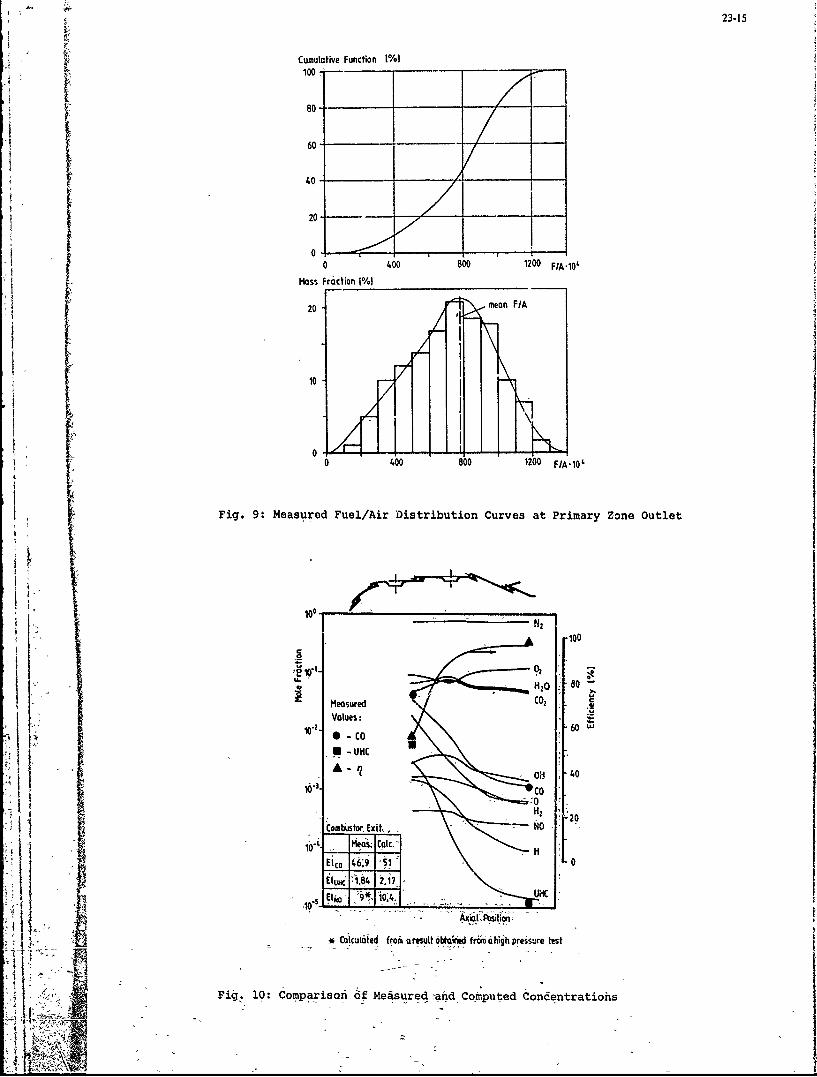
23.15

Cumulative Function 1%)100-

80--

60 ____ =40

10-

If0 A0 400 800 1200 F/A10'

Fig. 9: ~Masse FuelAion 1 itiuio%)vsa PiayZ eOte

100

4Z

0

- i'o -80

VuMeasured i010. .60s Col

* Coiedfo oeut bndfom hhprsrettILHCFig.~~~~~~~~~~~, 10 oprsn f40ue~adCmue Cnetaih

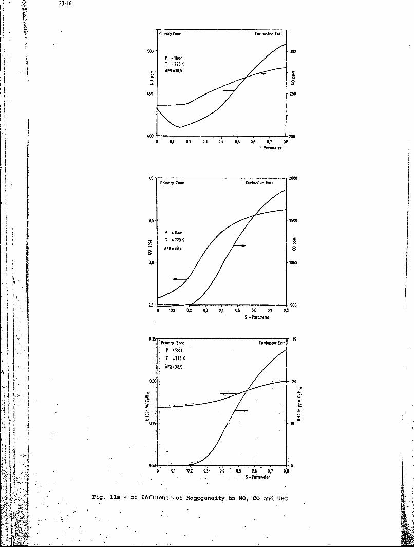
23-16

Primary Zone Combustor EMi

500 30DP .lbar

T -. 3r

0 0.1 0.2 0.3 0.A 0.5 0.6 03? 0.8

4.0 2000

!Pr~ory Zone Combusto Exit

T *773K

I-

0 1 0.21 0,3~ 0! 0,5 O0. 0,7 0.8

rI KB~ ~ ~ ~ ~ ~ ~ ~ ~ ~~~~~77 Ki.h ~C ifuhefNmgiet nNc n H

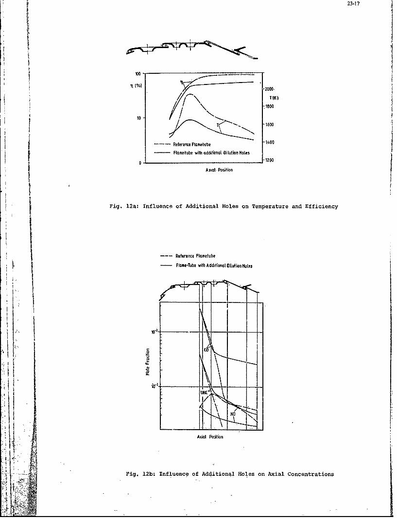
23-17

100

'1 l%1.2000,

TIK)

1800

1 10T -~1600

Reference Flometube -1400{ - Flometube with additional Dilution Holes

Axial -Position

Fig. 12a: Influence of Additional Holes on Temperature and Efficiency

I ~ Reference Floreetube- Rome-Tube with Additionol Dilution Holes

C

I N

~j ~ ;Axial ioition

I Fig 12b: Influence of Additional Holes on Axial Concentrations

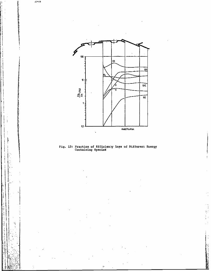
10

tC

IOIH

O'l ~ AxkIalPosition I

Fi.1:Fraction of Efficien-.y Loss of Different Energy

Fi.1:Containing Species'

4A, ___

i L23-i, ]

DISCUSSION

P.Gastebois, FrComment moddlisez-vous l'introduction de l'air de dilution? Est-ce un melange brutal ou introduisez-vous une loide melange entre l'air de dilution et les gaz en combustion?

Author's ReplyWe did not make an infinite mixing assumption for the dilution and cooling air. We look for the data of the airdistribution from a previous aerodynamic calculation and used a mixing law according to the equation:

mj = (x - xj)/(xM -xj)I" Mj

Mj total air in the plane (e.g. dilution air)x axial position downstream of the injection planexj axial position of the injection planexM mixing length of the jetsmj mixed fraction of air at position x

The mixing length xj was taken from previous water model tests.

Comment by D.T.Pratt, USThe coalescence/dispersion model fo reacting, segregated flow described in Paper 15 was devised in part, toovercome the difficulties of the Fletcher-Heywood "a"-model which is the basis of this paper.

The advantages are the following:

(1) Fuel and air need not be premixed and o-distributed.

(2) No a priori assumption w.r.t. residence-time distributions need be made.

(3) No special assumptions to effect recirculation-ignition problems are required.(4) No additional computational work is required.

(5) A single parameter (P vs a) controls both FIA mixing distribution, recirculation-ignition, and decayingexponential residence time distribution all of these advantages are gained by using a stochastic (C/D) vs adeterministic (a) model!I (6) Flame extinction (blowout) may be predictable.

J.B.Michel, NeWhat was the nitrogeit content of the fuel that you utilized and did you take into account the fact that you did not

' j :have a mechanism for "NO fuel" formation? Do you believe that your predictions of NOx are realistic?! [''::'Author's Reply

As the fuel which was us-.d for the experimental tests had no nitrogen content, there was no need to account for a"NO fuel" formation mechanism. But some other results from reaction kinetic calculations using the assumption,V" that the fuel bound N is present as free N atoms in the hydrocarbon decomposition phase showed the same trends

The NOx predictions showed good agreement with measurements taken from a high pressure test and scaled down

to atmospheric conditions by the well known pressure dependence (see Figure 10).

S.Wittig, GeDid you perform a sensitivity analysis of your model vith respect to the reaction kinetics? Is the resulting axialtemperature profile in agreement with selective measurements?

Author's ReplyWe did not perform a sensitivity analysis-with respect to the reaction kinetics vxcept for the vaporisation equationwhich has been included in the kinetics. Calculations showed, that this equation affects the unburnt hydrocarbons

"i with-increasing combdstor inlet pressure.

Themean exit temperature is ;n agreement with the measurements, but it is not possible to measure temperaturesby. thermocouples inside the combustor. Nevertheless the agreement of~primary zone efficiencies also reflect atemperature agreement.

24-1

' StEI-EMPIRICAL ORRELATIOINS FOR GASI ITURBINfE EMISSIONS, IGNITION, AND FIAME

STABILIZATION

by

A. M. MellorProfessor

tThe Comfstion LaboratoryPurdue University

West Lafayette, Indiana 47907, U.S.A.

SUINM4RYingFor operating conditions where the fuel evaporation rate is fast compared to the fuel vapor/air mix-

ing rate, a characteristic time model has been formulated to predict gaseous emissions and efficiency interms of combustor inlet conditions and geometry. The model, which involves kinetic and fluid mechanictimes, has been used to design low NOx burners, and study of several different conventional engine com-bustors suggests that the correlation may be universal. A related model, which includes a fuel drop]et

evaporation time, is being validated with data from laboratory combustors for spark ignition and leanflame stabilization. The preliminary application of this latter model to engine situations is described.

LIST OF SYMBOLS

A surface area of spark kernel at the quenching distance

a empirical constant

B mass transfer number for evaporation

cambient specific heat at constant pressureCpa pesr

D disc diameter

Damkbhler number at blowout

Dco Damkhler number for 00 oxidation

Dno Damk6hler number for NO formation

d tube diameter

dcolmb combustor diameter at quench locati,,n

do Sauter mean diameter of fuel spray

d quenching distanceqEmn minimum spark ignition energy

EI emissions index (g pollutant/kg fuel)

ka ambient thermal conductivity

A I co effective 0O quench iength (+ dco -

co quench +comb~Zi,quench air addition site where species i quenches((noqunc/CsO- di -

effective NO quench length c + dcomb

pri length from fuel injector to primary air penetration jets

'c6mbus6rair -flow rate

m4z primry zone bir flo rite

I: IP - combustor -inletpressureQi lower heating-valu of species i

4, R univ6rsal* ' constantI r cdrrlation 'coefficient

T. absolute teaperature

an -- Si t 1-

Tco Y --C'okidatin. empeatre C(.85Tin + =IsT¢), eF:-Tco in... .-. .

24-2

Ti inlet air temperatureinT efficiency oxidation temperature (Min + .T

T burned gas temperature at equivalence ratio 4

To=, adiabatic stoichiometric flame temperature

V mixture velocity in spark gap

Van n air velocity in plane of flameholder

! V, fuel injection velocity

Vref reference velocity at maximum combnustor cross-sectional area

velocity estimate in NO forming region

a ambient thermal diffusivity

effective evaporation coefficient

AT I stoichiometric temperature rise

nc combustion efficiency

0 air swirler vane angle

Pa ambient density

ya standard deviation from least squares fit

co characteristic time for 0) oxidation

characteristic tim for fuel evaporation

Teb (TTeb/Tin)

T Tfi characteristic tim for fuel injection

"h (fi/Tin)

hc characteristic time for fuel ignition delay

Thc (Thc/Tin)

Tno characteristic time for NO formation

" sZ characteristic time for heat conduction

T stco 0) oxidizing eddy lifetime

Ts~n NO forming eddy lifetime

T kinetic time for combustion efficiency

0 overall equivalence ratio

O @t prechaber equivalence ratio

1. INTRODUCTION

Gas turbine combustor design engineers would find extremely useful, quantitative models for combustionefficiency, emissions, flame stabilization, smoke and radiation, ignit'ability and altitude relight, andexit temperature ' traverse quality. Air lading correlations have frequently proven convenient for some ofthese performance parameters ihen combustors are of dissimilar scales but identical geometry and when mix-ing of fuel' vapor with air occurs fibre slowly than th6 .rate of fuel evaporation -(i.e., aviation specifica-tion fuels with properly de signed.atomizers). Lefebvre and do~aworkers (1,2) give-examples of these scal-

ing paraieters, which currently are ifi idde use by inddstry, for combustion efficiency and the blowoff

Howeveriboth the current interest in low emissions combustors of exotic geometry (3) and the de-graded fuels to be available ,in the' future (4) require extrapolations of these models, and-in some cases

d. Thus there is substantial reason to devel-o1ful properti uolude mre explicitly the effects -of combstor

bt nyears ago, n response toa growing concen oyer aircraft air,pollution, a number of chemicalreector" ntwork moe~ls were constructed -(5,6). Chemical kinetics were emphasized since it was known that

e pgltants were not in local-equilibrim, in the comtustor exhaust .plane, and the.fluid mechanics wex2d sies or palalel flow modules consisting of perfectly or partially stired, and plug flow re-

ators, The fuel spr'y in Jit liqud -for was usia gnored. Generally speakn, the -ndels were too

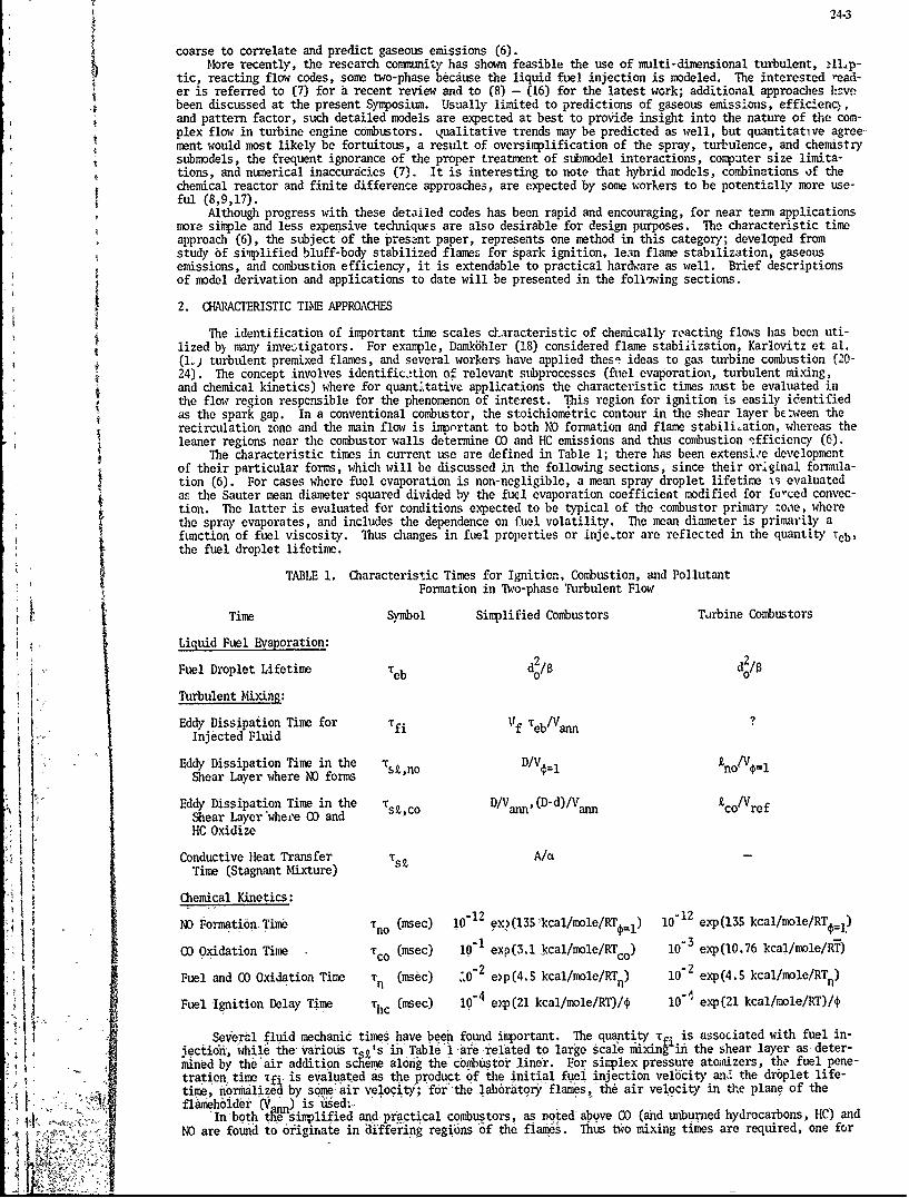
) 24-3

coarse to correlate and predict gaseous emissions (6).More recently, the research community has shown feasible the use of multi-dimensional turbulent, allp-

tic, reacting flow codes, some two-phase because the liquid fuel injection is modeled. The interested read-er is referred to (7) for a recent review and to (8) - (16) for the latest work; additional approaches 1-ve

4 been discussed at the present Symposium. Usually limited to predictions of gaseous emissions, efficienc),and pattern factor, such detailed models are expected at best to provide insight into the nature of the com-plex flow in turbine engine combustors. qualitative trends may be predicted as well, but quantitative agree-ment would most likely be fortuitous, a result of oversimplification of the spray, turbulence, and chemistrysubodels, the frequent ignorance of the proper treatment of submodel interactions, computer size limita-tions, and numerical inaccuracies (7). It is interesting to note that hybrid models, combinations of thechemical reactor and finite difference approaches, are expected by some workers to be potentially more use-ful (8,9,17).

? Although progress with these detailed codes has been rapid and encouraging, for near term applicationsmore simple and less expensive techniques are also desirable for design purposes. The characteristic timeapproach (6), the subject of the present paper, represents one method in this category; developed fromstudy of siplified bluff-body stabilized flames for spark ignition, le.n flame stabLlization, gaseousemissions, and combustion efficiency, it is extendable to practical hardware as well. Brief descriptionsof model derivation and applications to date will be presented in the follo3wing sections.

2. CHARACTERISTIC TIME APPROACHES

The identification of important time scales c.aracteristic of chemically reacting flows has been uti-lized by many investigators. For example, Damk6hler (18) considered flame stabilization, Karlovitz et al.(1Lj turbulent premixed flames, and several workers have applied these ideas to gas turbine combustion (20-24). The concept involves identific.,tion of relevant subprocesses (fuel evaporation, turbulent mixing,and chemical kinetics) where for quantitative applications the characteristic times m.ust be evaluated inthe flow region responsible for the phenomenon of interest. This region for ignition is easily identifiedas the spark gap. In a conventional combustor, the stoichiometric contour in the shear layer be:ween therecirculation zone and the main flow is important to both NO formation and flame stabiliation, whereas theleaner regions near the combustor walls determine 00 and HC emissions and thus combustion efficiency (6).

The characteristic times in current use are defined in Table 1; there has been extensire developmentof their particular forms, which will be discussed In the following sections, since their original formula-tion (6). For cases where fuel evaporation is non-negligible, a mean spray droplet lifetime is evaluatedas the Sauter mean diameter squared divided by the fuel evaporation coefficient modified for fo-ced convec-tion. The latter is evaluated for conditions expected to be typical of the combustor primary zoae, wherethe spray evaporates, and includes the dependence on fuel volatility. The mean diameter is primarily afunction of fuel viscosity. Thus changes in fuel properties or inje-tor are reflected in the quantity rob,the fuel droplet lifetime.

TABLE 1. Characteristic Times for Igition, Combustion, and PollutantFormation in Two-phase Turbulent Flow

Time Symbol Simplified Combustors Tarbine Combustors

Liquid Fuel Evaporation:

Fuel Droplet Lifetime d 2/8 2/0

Turbulent Mixing:

Eddy Dissipation Time for ?

Injected Fluid fi /f eb/Vann

Eddy Dissipation Time in the Tst,no D/V€=1 no/V =lShear Layer where NO forms

Eddy Dissipation Time in the T D/V ann, (D-d)/Varm tco/VrefShear Layer'whece 00 and s2,c°HC Oxidize

Conductive Heat Transfer T s£ A/aTime (Stagnant Mixture)

Chemical Kinetics:

"i : No Formati6n. Time no (msec) 1 2 ex? (135 kcal/mole/RT¢=1) 10" 12 exp (135 kcal/mole/RT¢=1)CO Oxidation Time co (msec) 10 exp(3.1 kcal/mole/RTco) 10- exp(10.76 kcal/mole/RT)

K Fuel and CO Oxidation Time rn (nsec) "0"2 e~p(4.5 kcal/mole/RTn) 10-2 exp(4.5 kcal/mole/RTn)

U Fuel Ignition Delay Time 'hc (msec) 10"4 exp(21 kcal/mole/RT)/O 10- exp(21 kcal/mole/RT)/

Several fluid mechanic times have been found important. The quantity Tfi is associated with fuel in-vjectioi', while the various z£'s 'in' Tab 1A are related to large scale mixing in the shear layer as- deter-

mined by the air addition s eme along the' cbmbustor liner. For simplex pressure atomizers, the fuel pene-tration, time Tf. is evaluated as the product of the initial fuel injection velocity and the droplet life-.time, nrmlzed by- some'air velocity; 'for'"the air velocity in the plane of theflaMehbider (V ) is used;a

J, , , In -both t!W Simplified and practical combustors, as noted above CO (and unburned hydrocarbons, HC) andNO are found- to 6riginate in differing regions of the flames. Thus two mixing times are required, one for

24-4

each species. Both are defined in terms of a significant length, a function of combustor geometry, and acharacteristic velocity, given by the combustor inlet conditions. Particulars will be reviewed in the sec-tions to follow. Last, for the special case of ignition in quiescent sprays T has been defined as a heatconduction time, the ratio of the surface area of the spark kernel evaluated a the quenching distance tothe thermal diffusivity of air.

Four kinetic times, all in Arrhenius. form, have been found useful. They describe the rates of NO for-mation (tnq),. 0.oxidation (Tco), fuel and 0) oxidation Jumped ito correlate combustion efficiency (T.),and an ignition delay time for flame stabilization (Th ). This last time includes the equivalence ratioexplicitly since at the lean limit the rate is expecte5 to be first order in fuel concentration. The acti-vation energies aid choice of reaction temperatures for all of the kinetic characteristic times are deter-mined from combustor inlet temperature variations; the pre-exponential factors are chosen so that the ki-netic times are of order of msec. Note that these kinetic times are primarily a function of combustor in-let conditions, overall equivalence ratio, and fuel heating value.

Thus fuel properties, dobustor geometry and inlet conditions are all included in the characteristictime model. Appropriate combinatiois of these times should therefore correlate the spark ignition and leanblowout limits, 0 and NO emission indices (g pollutant/kg fuel), and combustion efficiency. Note that allof the characteristic times are chosen only to include the expected trend with a variation in fuel, corn-bustor, or cycle design, and of course are not exact quantities. Hence qualitative trend can be encom-passed in the model, but experimental data are required to quantify the model, which is thus semi-empirical.As noted previously, success requires recognition of that portion of the combustor flow limiting to thephenomenon of interest. In the following sections we chart progress in model validation.

3. SPARK IGNITION ANDFLAME STABILIZATION

The scabilization of premixed turbulent flames can be thought of in terms of the 'elevant DamkbMilernuber a constant in the limit; specifically, for 'Damkbhler number taken as the ratie of a turbulent mixingtime to an ignition delay time, the, limit is defined when the ratio equals unity:

A > 1 stableDbo - s,co hc < 1 unstable (1)

This criterion simply states that the residence time (replaced by a turbulent fluid mechanic time followingSpalding (25)) precisely equals the fuel ignition delay time at the limit. Recognizing that neither ofthese characteristic times can be estimated exactly in a cobustor, Eq. (1) is replaced by the limit equa-

tszco " 'hc ' (2)

Zukoski and Marble (20), and more recently Altenkirch and Mellor (24), have argued that both times inEq. (2) must be evaluated in the shear layer between the fresh air and the recirculating fuel/burned gasmixture. Zukoski (26) further discusses Eq. (2) for two-dimensional and axisymnetric flows; we limit ourattenion here to the latter case, Note that Thc must be evaluated at the highest flame temperature attain-able in the flame, since the corresponding physical regions of the flow will be the last to extinguish.

a. Premixed Turbulent Flames (Afterburners) - Lean Blowoff

Plee and Mellor (27) have used premixed turbulent flame stabilization data obtained by Ballal andLefebvre (28), for the bluff-body flameholder depicted in Fig. IA, to quantify Eq. (2). For inlet temper-ature variations from 300 to 575 K'with gaseous C3 8 as fuel the apparent activation energy in whc wasfound to be 21 kcal/mole. Acceleration of the reactants as they flow past the recirculation zone was ac-counted for by a density (i.e., temperature) correction to the velocity in the plane of the flameholderVann, so that

TStco = (D/Vann) (Tin/T) (3)I + i

I0 hc 10 4 exPo21 kcal/mole/RT)/ mec (4)

and the blowoff limit condition becomes

XS9"CO Thc (T]Tin)- c()

In the abore D is flameholder diameter (a measure of t!ie length of .the recirculation zone), and Tin is in-let temperature+0f the premixed reactants. As was noted the kinetic temperature T in N. (3) through (5)mustbe evaluated'at" he maxirin temperature available 'in the system) so it is taken as the adiabaticI) flime temperature at the approach equivalence ratio 4.

The blwoff mit correlation is shown in Fig. 2 for the premixed data of Ballal and Lefebvre (28).The limit e ti~n given in the figure -is

' - s.,co =2,11 lc' - 0.46 (6)

where T and. 4 are evaluated just prior-to blowoff. Operation at conditions above the least squares line isstable, and- in Fig. 2 it is sh6wnfiow-ohe' can approach thet"limit by either increasing the inlet velocity ordecreasing th6 equiyalnce ratio. 'The quantity r i1sa '6zrel'tion' cefficient (r = 1.00 is perfect), and

'y, is the' standard deviationi (27).N6te. that. co ,irlation (6). does:'not include the ipprachfl6w turbulent intensity explicitly,, as do__. othe' correldtions(28). -Most likely some of 'the scatter of Fig. 2 is du to neglect of intensit varia-tions, bt' sict; turbuleficb jpaamet'rs ate rarely known in the-practical ,case. a direct correlation "in,

z ters.of inile elocity Vnis preferred. Als', turblence- ceistiyA interactiofin (26) are ignored sincesb, tutu nce ' ' istr in."

24-5

recirculat :0-e Dana by Rnilal a., Lefbvlre (28)

fuel * air 9.6

- -- - s ~ r l a v eL e a n B l o w o f f Li m i t"---r .. . . . r flwie 8.4 /

Confipuration A Balll and Lefebvre (28) STABLE

7.2

- .... recirac2atio, =~e 6.0--r __ _ ?± I v 0' UNSTABLE

8 3a ) e r L e 4 . 8

Conf pration 3 Pl. and Mellor (3Z) 3.6 0 2.11.c .46

a 0-X 0 (r .93 72 data

2.4 oredca~-~ation:ve ufgatnA

air

Iharlyer ilane

Configuratlon C lee and .ilior (32) 0 . 1.6 2.4 3.2 4.0 4.8(neglili e hetero~ene s effecs) IL (rjec)

Figure 1. Schematic of three simplified bluff Figure 2. Characteristic time correlation forbody stabilized flames. lean blowoff in a bluff body stabilizedflame burning gaseous propane (Fig. 1A).

fluid mechanics and reaction rates are treated separately in Eq. (6). Because the apparent activation en-ergy is determined empirically, perhaps its value reflects these interactions since it is different frompure kinetic values defined in a similar spirit (29,30,31). In any case Eq. (6) provides a design toolwhich incorporates variations in flamoeholder geometry and inlet conditions.

b. Partially Prevaporized and Premixed Flames (Prechambdr Combustors) - Lean Blowoff

For Configuration B of Fig. (1), data obtained'by Plee and Mellor (32) have also been correlated (27).Fuels testedwere liquid C3f 8 , which flash evaporates at the inlet conditions, and Jet A, which partiallyevaporates in the fuel p:reparation tube,? designed to minimize the posibility of flashbrck (33). The pres,ence of liquid fuel was found to narrow the lean limit due to the time required for evaporation; therefore

Cq. (S) bucomes (27)

skco Tc + aTeb (T/Tin) (7)

+ a(8)

where the quantity a must be detemined empirically. Eq. (7) and (8) imply that the fuel ntust partiallyevaporate before 'th. homogenebus kinetics ,afi lead to ignition.

The characteristic length for Configuration B is disc diameter less tube diameter, and ThC is definedby Eq. (4) with * the tube equivalenice ratio ( ) and T the mean of (T + Tim) or (T = + Tin) for 4 t > 1;T b is given in Table 1. A result similar to tat shown in Fig. 2 is gfven by Plee ad ellor (27) witht&e correlation

T s =,co 2.24 (TAc + 0,011Teb) + 0.06. (9)

Note rhat the empirical value of the constant a in Eq. (9) has no physical sighificance since the charac-teristic times are only order-of-magnitude estimates; however, liquid, fuel properties and injector designare not implicitly included in the model via teb,

c. Liquid Fueled Turbulent Diffusion, Flames with Negligible Fuel Penetration (Conventional Combustors)

- Leat Blowoff

lee aid-elior '(32) have in addition reported data for Configuration C -in Fig. 1. In the case wherefuelp'penetration is 'negligible (upper flame of'Fig.. 3),.'the.-.fl'a '_is-mixing controlled, that is, the rateof mixihg' of fuel vaporwith -air, rathei than 'the evaporation.rate of liquid fuel,. detenifies the heat re-lease rate (34). This is' the-situati0, ousIually encunterd.ihpracfical i vdntion l combutors buerningaviatiIon -specification fubis with p6per 'injectioh ,tecfini4ues (35). 'Kinetics,; of' 66urse, influence themixingdo iatd flame. If T inEq. (4)' is takefi as the adiabatic,.st'oichioinetric flame temparLture T

s:in~ai i flame) andan the overalAy equivalence atiooat blowo

7sco' = l4 'ic + 0.ocb) +0 08. (10)

Note the similaritiesof Bq. (9) and (10). In fact all three cenfigurations of Fig. 1 can be correlateJ

,."tZM

f~ ~ 'X NJ_____________________ 1! -593 N:.-c (So , So : Irvs.~

_________________________3.2 W < T1 , 160

Air

CA strla rfa 2.8 0 Disc Din - 11.43 ca~, Jet Aa0isc Din-8.89 a-,Jet AO11i~c Din - 6.99 cm, Propm~

Disc2.4

lqui F=L2.0

- - - STABLE ElNegligible Fuel Penetratic. Ef-iects E(ee

shear la~er free ste±- 1.2 UNSTABLEIfi (00 M T .90 67 d3ta

r-uj

M ,%.Lquid Fa:1 .414 (f-AMt 0-O p a

sL co *14 0I., 0

Fuel Penetration Effecs Important 0 _ __ .6 .9J

Figure 3. Burner schematic illustrating the effect Figure 4. Characteristic time correlation forof fuel penetration on flame structure, data obtained on the disc-in-duct

(Fig. 1C) flameholder (negligible

together: the result is shown in Fig. 5 with the universal fueopertrtinaefecs)

stc 1 . 8 2(Thc + 0.011'b + 0.04 (11)

where the terms used in T c depend on flameholder design and those in Tc on the nature of the flame(premixed, partially prevap6rized and prendxed, or unmixed liquid fuel anh~ir).

Eq. (11) gives the lean blowoff limit in tems of "variations in pressure, inlet temperature, refer-ence velocity, flameholder geometry, housing diamuter, fuel type, and injector size . . . Kzowledge of theflameholder configuration inlet conditions and atomization determines T..Z and Tb;fo thsr caeasily be computed'that is a function of the inlet 'conditions and the b owoff equaiValence ratio. The blow-off velocity is also calculated in a similar fashion if the geometry, pressure, inlet temperature, atomiza-tion, and equivalence ratio are given. In addition, the correlation can predict simple flameholder modifi-cations necessary to optimize flame stabilization for a given operating condition (27).11

d. Liquid Fueled Turbulent Diffusion Flames with Strong Fuel Penetration - Lean Blowoff

For Configuration C of Fig. 1 with fuels of lower volatility or higher viscosity than Jet A, fuel pen-etration alters the structure of the flame to the case shown in the lower portion of Fig. 3, particularlyfor the smjaller disc diameters (27,32). ,Increased flame length associated with the fuel penetration on-hances the stability of the combustion process. 'Plee and Mellor (27) have shown that inclusion of Trfj.with all other termn definiedas in Section 3.c above, collapses these data as well, where

T fi Vf Te/am12)

j fi= fi (T/T.) (13)Here Vis the initial fuel injection velocity estimted from empirical information provided by Crowe (36).The il penetration effect ha ensown important when the ratio (T4i/TZ is greater than ten (27).The finial, complete correlationjis -sh inFg -ihtelimit equation

T .2'=2.*12(TI+U01 (14)s2.,co + fi hc Tb) + 0.095.

Fornegigbieful puetaton T'~ 0,6q. (14) compares favorably to Eq. (10) and (11), and for pre-mixed systems (Ti. :' t = 0) Eq. t14) is nearly identical to Eq. (6). The fuels utilized to develop Eq.( 14) ihlded JP, 4,. -A A, -DF 2, and Jet A blended ifth a small amounit of lubricating oil to give an in-I-I~~~~ crased eid'bo-iln Pint '(27 more- recently'model pidedictlbns f6r unleaded gasoline, J 0 o nJ ~ ~No.- 6, 6ils have beeii v~idated with, CoifigUiati~dr of Fig. 1 (37). These flaw~s, with strong fuel pen-ertdi6ff~cts;j ar6 'thoighi to be apuroahiig, the te ii nsrycmutoweetefe vpfloration raede teimines-the h eat release rate.

The f uelI- rpii~ion effect 'is not a tkiatd to -occur in conventional combustors operating withaviationi 46eif1'cat1o'fue&ls. Thubs Eq .(14) with f.= 0 has'been used fdr blowoff data (38) for the T-63

coneriioalcbbus6 (39'.Using the definition of TsX co given in Table I for practical com~ustors

sZ,cO tc'-ewhere

vl

STABLE9.6 9.6

, 9.6 O .6Lean B ff L 0

Lean 31o.,of Lliiz .8.4 8.4

Configuration Configuraticn7.2 0 A Fig. IA 0 7.2 0 A Fig. 1A

0 B Fig. 1B 0 3 Fig. 1

6CFig.

ic

AC Fig. Ic 6.06.0 0

i ., € STABLE 0 0

4.8 0 4.8 UNSTABLE*0 0 0

UNSTABLE5.6 A 3.6

/0 0 0

" o 8

". It.c -1.82 (N -. 042. .040

-.93 .O0 data

oy - .36 .2 Tst.00 *.1t 2.12(T~c - '111;b)1.2 .06 .09

397 data

1.6 2.4 5. 4.0 4.8 . $ 1.6 2.4 5.2 4.1 4.8

rI: .011 re (rscc

Figure 5. Complete characteristic time correlation .o1 b (FeS)for inlet, geometry and fuel variationson three simplified bluff body stabi- Figure 6. Complete characteristic time correla-lized flames (negligible fuel penetra-, tion for blowoff limit.tion effects).

-1l -1 -1Pco = Zpri + dcomb (16)

(see (35)), tri is the distance from the fuel injector to the centerline of the primary air penetrationholes at combtstor diameter dcow, and Vef is reference velocity, Eq. (14) with Teb also taken as zero wasused to compute the three points to the left of the limit in Fig. 7 for Diesel fuel 2, Jet A, and JP-4,respectively.

Then, using estimates of Sauter mean diameter do given by Moes (38) and Eq. (11) including the T h

term, the points to the right of the limit in Fig. 7 were established. Note that the ordering of the fuelsis now reversed. Clearly, ;reasonable choices of do for each fuel could be selected which would align allthree fuels exactly with the lean limit Eq. (14). Hence one provlem in application of the characteristictime model to practical combustors appears: Sauter mean diameter is required in some cases at the engineoperating point (elevated temperatures and pressures), a nunber not usually available.

However, Bq. (14) with Tfi = 0 is recommended forengine applications; a preliminary model test is shownin Fig. 7. Further model validation will proceed withadditional turbine combustor blowoff data.

2.8 STABLE e. Stagnant Sprays - Spark Ignition

Construction of a related model for spark igni-b. (14),-0 tion is in progress (40). First efforts have involved

,4 a , 4.. / "n im u m i g n i t i o n e n e r g y d a t a o b t a i n e d y B a l l a l a n d

Lefebvre (41) for quiescent sprays of several fuels.Recognition that to first order the ignition of a

2.0 without Ti !th ' b spray is evaporation limited (42) greatly simplifies, 2 model development.

( ec ) 2 J J / J S t a r t i n g w i t h E q . ( 8 ) w i t h o u t t h e v e l o c i ty c o r -1.6 - DJ4rectiofi due to combustion (the mixture is stagnant),

.2 UNSTABLE TsZ " Th + aTeb " (17)

Neglecting kinetics in favor of evaporation means

.8aTeb hc

hc

(18)

.4 so that the ,spark ignition limit is given by0 6 I - T S

b (19)

.2 .4 .6 ; 1.0 1.2 where TsZ must be -redefined for a stagnant, mixture;

.011.1; (*) the heat source is 66w :6e spark rather thin an- idja-cent iecirculatio n "zone.

Figure 7. Application of flame stabilization Heat loss by conduction, as opposed to turbulentmodel to conventional combustors. convection, will' c6n ete with the heat ddition from

the spark which drives the evaporation (40). Hence Tst for this special case is given by

(20s = " dq PaCpa/ka (20)

where dq is quenching distance related to mininun spark ignition energy E1 n via

dq = {Emin/ 4 acpaAT=l }I / 3 . (21)

Other properties which appear are ambient gas density (Pa), specific heat (cp ), and thermal conductivity(ka); ATb= 1 is the adiabatic stoichiometric temperature rise associated with the droplet or spray diffusionflaihe after ignition.

One other modification to Eq. (19) is required. Mat limits ignition is the vapor phase concentrationof fuel vapor, which can be increased by decreasing Teb. However, increasing the total number of dropletsby increasing the equivalence ratio will also increase the spray evaporation rate linearly. This effect isincluded by altering the Teb term so that the ignition limit becomes

Ts. A, Teb/' (22)

If the quantity d. is computed from the data reported by Ballal and Lefebvre (41), and Eq. (22) istested, then Fig. 8 results. Excluding for the moment the flagged data (the points near the origin aredata with symbols omitted for clarity) the fit is linear and the y-intercept is near zero, ai$ predicted bythemodel, with the ignition limit given by

T 14.2T + 2.29. (23)14*2 eb/4

How changes in spArk energy, Sauter mean diameter, and fuel volatility (B, the transfer number) affect astable operating point are shown in Fig. 8.

Fig. 9 demonstrates the correlation in terms of Fmin versus 4 for one fuel (dashed lines are from Eq.(23)) and explains the deviation of the flagged data ron the fit dn Fig. 8. All of these points are forthe lowest equivalence ratios, which tend to negate Eq,. (18). Thus the kinetic time for ignition must beevaluated and included in a complete modl; this work is currently underway. In addition, prelimdnarystudies of data for flowing sprays with the conventional definition of Tst (dq/V), neglecting kinetics,show similar agreement as in Fig. 8 (43). Of course, turbine combustor model evaluation is the eventualgoal.

(Ta too L-cn -.0Iat

1400 0 I-octane ( 100 I -ctano - 1 atmADiesal oil .

D heavy fuel o0,1

120 0.2 <P <1.0 101200 - --. " -.

20'< do !170m vn aSi~0.43,1 4 ;L 1.o0 0"-

Igo0 "i -," 6.93 0/ .0

100u

IGNITION Limit 10 -L0

Boo do Ji @

-( NO IGNISTION

600 t

* 0400 0, "at 14. 2.°29o

SCharacteristic -ime corrdaton fo0 Via

heignition~ ofquiesdenti fuel spray's Figure 9. Minimm ignition energy of quiescent

-(data'froi Ballal ° ahd-Lefebvre (41)). mixtures for various drop sizes (data

• fromBallal and Lefebvre (41)).

5 (3)an fo c~venioha cob6 cor (3, 4,S, 6,4). - Forthesecondtflane in Fig. 3 and for cohfigur-"F6r nitrfd ox~ide inomiiifi controllddsituations it canabe shown "(34,47) tat the NOv emission index

(g as N)2/kg Eiiel):'wil1-scadelinea1li :withthe r61e~ant-Damk~5hler nuinber:i

o .99 (43

T'l"" 27.,o, s~o~

.iEq. (24) states that an increase inNO-forming eddy lifetime (r n) will increase NO emissions linearly.The inverse dependence on rno reflects that increases in T =1 (rae 1), which decrease Tno, also increase

it is the formation of NO which must be quenched in gas turbine combustors, whereas 00 (and HG) is

limited by quenching of its oxidation reactions. Thus the functional dependence of ODE! is the inverse '0i that for NOxEI (34):

COhI -,D Ar (25Sco corsic (25)

I Here long eddy lifetimes and high temperatures decrease 00 (and HG) emissions.If OD and HC concentrations are proportional to one another over the range of data to be correlated,

then it can be shown that (48)100 - -l Dl 1 nlP , (2f)

c ~ st,cowhere combustion efficiency nc is obtained from (49)

100- Mc(%) = {(GOEI)Q + C (27)c co + HGEI)Qhc)/ 1 0Qfuel

The Q's are the lower heating values of the indicated species.

Finally, for cases where fuel penetration is important, no fuel independent correlation han yet beenachieved (48). Although this case may not be significant in gas turbine applications, it can representthe situation in boilers utilizing residual oil or pulverized coal.

a. Liquid Fueled Turbulent Diffusion Flames with Negligible Fuel Penetration (Configuration C)

Emissions and Efficiency

Probing of the flame shown schematically at the top of Figure 3 (50) demonstrated that CO (and HG)quench at the outer but leading edge of the shear layer, while NO forms on the centerline of the flame down-stream of the recirculation zone. Consequently the eddy lifetimes were taken as

T sk,co = D/ann (28)

and

wrT stno "DIV =(29)

where

V 1 V l + T /r.n (30)

As before, the kinetic tinmes were determined from inlet temperature variatiuns, and slightly different def-initions from those of Table 1 were used in this early work (34). Here T is the burned gas temperature atthe overalleeqivalence ratio ta

For liquid C3H8 as fuel the NO and CO correlations are shown in Pig. 10 and 11, respectively; bothcurves are linear a the model predicts. Note also the near zero y-intercepts and the good correlation co-~efficients. A similar combustion efficiency correlation for the mixing controlled case is shown in Fig, 12,

fdr"several additional fuels (48). In the latter case- is given in Table 1, where

n = 9gTin + T(31)

The respective least squares fits are

NOEI 0.68rI,,noTno +0.36; (32)

,OEI 17.9TCo/-s,co + 3.4; (33)

100 - nO(%) '2x4rT/TSXC o - 1.69. (34)

For, negligible fue penetration these equations give emissf.'ons and efficiency in terms of inlet conditions,flamehol1de geo6iietry, ,d fuel heating value. They bave been utilized to design the optinmal disc-in-,ductburner config'iatibii6-whih e hib;it' miGiml-O emissions (34).

b. Li Flames with Negligible Fuel Penetration (Conventional Combus-

tors)' 1 iisidfis

Cohsiderable utilization, of the characteristic time model has occurred for gaseous emissions fxom con-enti6nal dbiiut6r (6 i35,44,,5,647). The most reent iork (46), has dealt with the Pratt and Whitney

JT9D fid'shown that identical ¢orlations. can be obtained with the .cobustbrs analyzed previously, theGT- 309 'vehicular and T-63helicbpter b ers.

For most cases d-oplet evapoiation-can be assumed rapid compared to the kinetics and air/fuel vapormixing (35,44); hence NOx and 0) emissions are expected to correlate with Eq. (24) and'(25). The defini-tions of the kinetic a nd-nuxng'times. are given in Table 1, but the mixing times differ from those of Con-figuration IC due to th'e more" compiicated ge6met-of the gas tudibie combustor (46). Here best correla-

tions. a-e obtained-with.

ncose) + (35).i 11o No,quench dcomrb

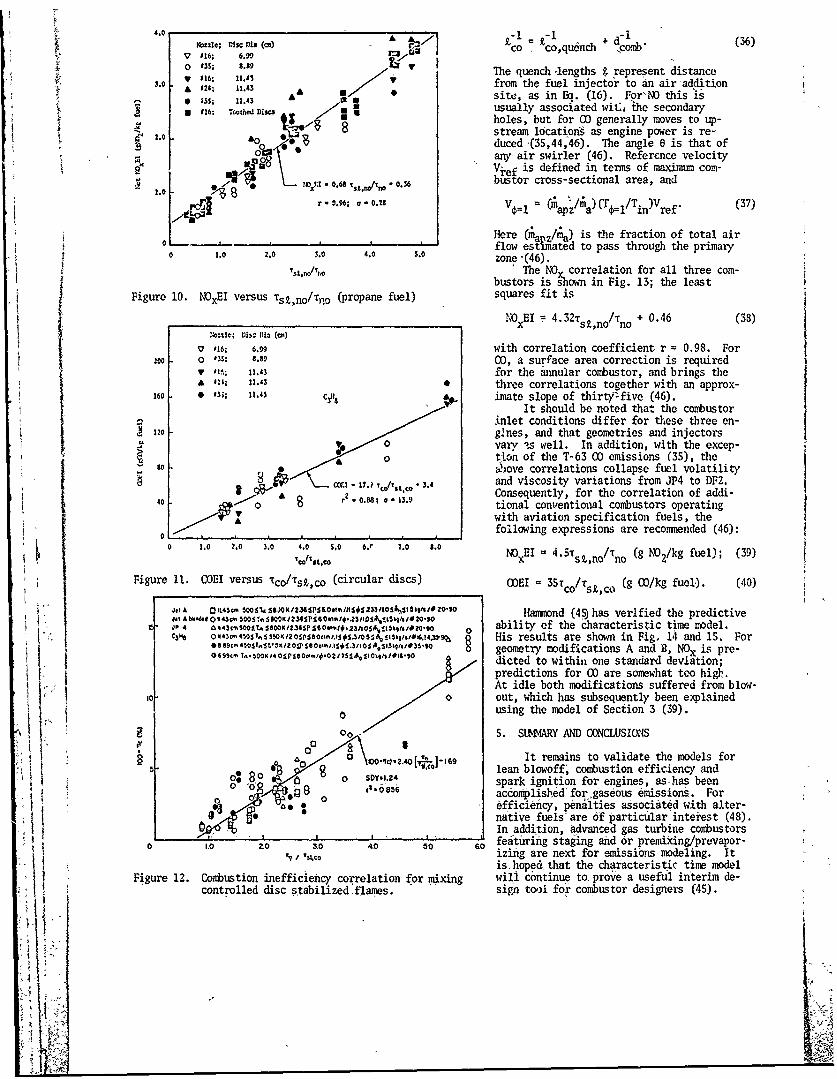
4.0 • -1 = -1V 016; .99 (.) co co,quench + corb'

0 ,13; 8.89 V The quench ,lengths P represent distance016; 11.43 from the fuel injector to an air addition.site, as in Eq. (16). Far'NO this 'is

#16: T11.e A 1 a usually associated wit], ,the secondaryp 1 tLholes, but for CO generally moves to up-

: . " 8 stream locations as engine power is re-any air swirler (46). Reference velocity

V-ef is defined in terms of maximum com-1.. - 0.68 . bustor cross-sectional area, and

r - 3.96; a- 0.2 V :1 = ( az/Ma) (T =i/Tin)Vref. (37)

Here m a is the fraction of total air0 L . flow estnated to pass through the primary10 1.0 2.0 3.0 4.0 s.0 zone (46).

, 'The NO correlation for all three com-bustors is shown in Fig. 13; the least

Figure 10. NOxEI versus Tspno/Zno (propane fuel) squares fit is

NOxEI = 4.32Tsi,no/Tno + 0.46 (38)Nozzle; DiC Ilsa (m)

V :16; 6.09 with correlation coefficient r = 0.98. For1o0 0 3S; 8.89 0X), a surface area correction is required

T #M; 11.43 for the annular combustor, and brings theA ,-'; 11.43 0 three correlations together with an approx-

160 ,3i; 11.43 CA 31. imate slope of thirti'-five (46).It should be noted that the combustor

inlet conditions differ for these three en-120 gines, and that geometries and injectors

0 vary izs well. In addition, with the excep-0 tion of the T-63 0) emissions (35), the

I)ove correlations collapse fuel volatilityr, - 11. , 3.4 and viscosity variations from JP4 to DF2.

40 r2 -o. o 13., Consequently, for the correlation of addi-

3. tional conventional combustors operatingAwith aviation specification fuels, the

_________________________ following expressions are reconinended (46):

0 1.0 2.0 5.0 ,0o s.o . 8. NOxEI = 4 .Ssg,no/Tno (g NO2/kg fuel); (39)

Figure 11. COEI versus Tco/Tsg,co (circular discs) COEI = 35r /s,c o (g 0)/kg fuel). (40)C Lco

JeI A 011.43C 5OOSU Ilt$/@ 20 t Hamond (45) has verified the predictiveJet A -4000 1143v" 500 S ."5 OKI 236P i 6O lOt1.3ID0, L5o .14/s Ias f0-0! JP 4# = Ao xl234SP$60,,.,#.=31o ,:,=l,,*tQ. o 0 ability of the characteristic time model.S1C 3.8 oM 4340S 5o5X2 0 o58 4..5.30.% I5 t 0,,4%bS His results are shown in Fig. 14 and 15. For

* 9c. 4 50ST. 12 OTS00"1.1#.3 /1,15 i~ s 1. 3590geometry modifications A and B, NOx is pre-+ 603,c, ,.'.100K,4o Pi8eoo*.Ol/?51.o b,,.t,,I.0 / dicted to within one standard deviation;

predictions for 00 are somewhat too high.At idle both modifications suffered from blow-

1 out, which has subsequently been explainedusing the model of Section 3 (39).

O S SMARY AND CONCLUSIONS

0 It remains to validate the models for0: 0 lean blowoff, combustion efficiency and

~~: ao S O-. c 2.4~~hG- 6, 08.. o 0 spark ignition for engines, as-has been

00" eaconplishedfor gaseous emissions. Foro8 efficiefic, penalties associated with alter-

H native fuels are of particular interest (48).U -In addition, advanced gas turbine combustors

featuring staging and or premixing/prevapor-0 ,.0 Zo 3.o 4.0 0 0o izing are next for emissions modeling. Itis hoped that the characteristic time model

Figure 12. Combustion inefficiency correlation for mixing will continue to prove a useful interim de-controlled disc stabilized flames. sign to,)l for combustor designers (45).

1_ .

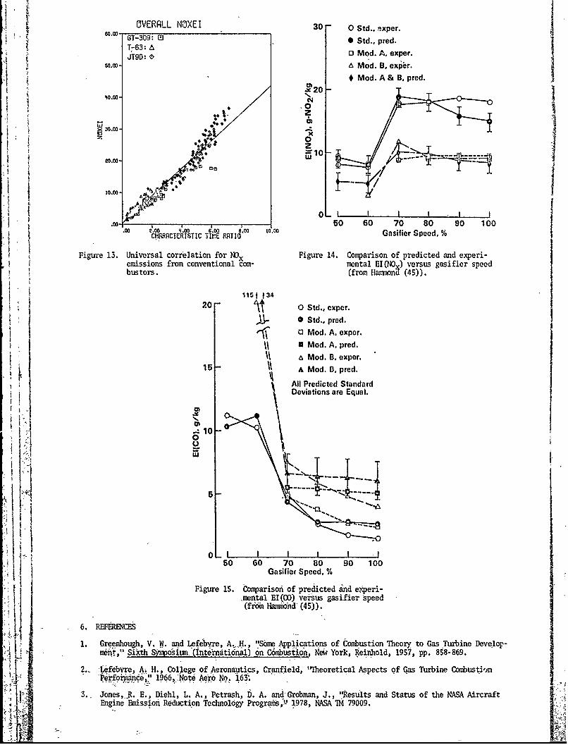
OVERRLL NOXEI 30 0 Std..GT-309: 9 Std.. pred.T;-63: &JTgD: 0 0 Mod. A, exper.

6.00- 'a Mod. B, expbr.

* Mod. A & B, pred.2 20-

.0

49~xz 00

A ' 1

oL I I ,.oo. so 60 70 80 so 100

CHRfCTERISTIC TIME RTIOGasifier Speed, %

Figure 13. Universal correlation for NOX Figure 14. Comparison of predicted and experi-emissions from conventional corn- mental EI(NO ) versus gasifier speedbustors. (from llanmon (45)).

115f f34

20 0 Std., cxper.

* Std., prod.

S 0 Mod. A. exper.U Mod. A. pred.

AI Mod. B, exper.16- A Mod. B, pred.

All Predicted StandardDeviations are Equal.

IS

.4 10 -

I0I I I ~ l

50 60 70 80 90 100Gasifier Speed, %

Figure 15. Comparison of predicted and experi--mental EI (CO) veisus gasifier speed(fizia Habmind'(45)).

6. REFERENCES1. Greenhough, V. W. and Lefebvre, A., H., "Some Applications of Combustion Theory to Gas Turine Develop-

2.. of o Gas TurbinentustinVent Siktl S~mosiumo (International) on Combustion, New York, ReinholA, 19S7, pp. 858-869.

2., ,4~febvre, A H., College of Aeronautics, Crarfield, Ir~neoretical Aspects of Gas Turbine Combustiin

-Perfo , '-ncI*" 1966, Not6 Aemr No. 163 .

3., Jones,_R. E., DiehI, L. A., Petrash, D. A. and Grobman, J., "Results and Status of the NASA AircraftEngine mssion Reduction Technology Programs,"' 1978, NASA 'IM79009.

4. Longwell, J. P., "Synthetic Fuels and Combustion," Plenary Lecture, Sixteenth Symposium (International)on Combustion, Pittsburgh, The Combustion Institute, 1977, pp. 1-15.

5. Mellor, A. M., "Current Kifietic Modeling Yechniques for Continuous Flow Combustors," Emissions fromContinuous Combustion, Systems, New York, Plenum Press, 1972, pp. 23-53.

tt 6. Mellor, A. M., "Gas Turbine Engine Pollution," Pollution Pormation and Destruction in Flames, Vol. Iof Progress in Energy and Combustion Science, Chigier, N. A., Editor, Oxford, Pergamon, 1976, pp. Ill-133.

7. Mellor, A. M., 'Turbulence Combustion Interaction Models for Practical High Intensity Combustors,"Presented at Seventeenth Symposium (International) on Combustion, 1978.

8. Swithenbank, J., Turan, A. and Felton, P. G.,. 'Three-dimensional Two-phase Mathematical Modeling ofGas Turbine Combustors," Project SQUID Workshop on Gas Turbine Combustor Design Problems, 1978.

9. Harsha, P. T. and Edelman, R. B., "Applicaticn of Modular Modeling to Ramjet Performance Prediction,"1978, AIAA Paper No. 78-944.

10. Novick, A. S., Miles, G. A. and Lilley, D. G., "Numerical Simulation of Combistor Flow Fields," 1978,AIAA Paper No. 78-949.

11. Mongia, H. G. and Smith, K., "An Empirical/Analytical Design Methodology for Gas Turbine Combustors,"

1978, AIAA Paper No. 78-998.

12. Jones, W. P. and Priddin, C. H., "Predictions of the Flow Field and Local (as Composition in Gas Tur-bine Combustors," Presented at Seventeenth Symposium (International) on Combustion, 1978.

13. Novick, A. S. and Miles, G. A., 'M odeling Parameter Influences in Gas Turbine Combustor Design,"1979, AIAA Paper No. 79-0354.

14. Bruce, T. W., Mongia, H. C. and Reynolds, R. S., "Combustor Design Criteria Validation. Vol. I. Ele-

ment Tests and Model Validation," 1979, USARTL-TR-78-55A.

IS. Mongia, H., Reynolds, R., Coleman, E. and Bruce, T., "Combustor Design Criteria Validation. Vol. 11.Development Testing of Two Full-scale Annular Gas Turbine Combustors," 1979, USARTL-TR-78-SSB.

16. Mongia, H. C. and Reynolds, R. S., "Combustor Design Criteria Validation. Vol. III. User's Manual,"1979, USARTL-TR-78-55C.

17. Felton, P. G., Swithenbank, J. and Turan, A., Sheffield University, "Progress in Modelling Combustors,"1977, HIC 300.

18. Damkdhler, G., "Einflfisse der Strmung, Diffusion und des WdrmeUberganves auf die Leistung vonReaktionsbfeu," Z. Elektrochem, 42, 1936, pp. 846-862.

19. Karlovitz, B., Denniston, D. W., Jr., and Wells, F. E., "Investigation of Turbulent Flames," J. Chem.Phys 19, 1951, pp. 541-547.

20. Zukoski, E. E. and Marble, F. E., "Experiments Concerning the Mechanism of Flame Blowoff from BluffBodies," Proc. Gas Dynamics Symposium on Aerothermochemistry, Northwestern Univ., 1956, pp. 205-210.

21. Mellor, A. M., "Simplified Physical Model of Spray Combustion in a Gas Turbine Emgine," Comb. Sci.i Tech. 8, 1973, pp. 101-109.

22. Gouldin, F. C., "Controlling Emissions from Gas Turbines - the Importance of Chemical Kinetics andTurbulent Mixing, " Comb. Sci. Tech. 7 1973, pp. 33-45.

23. Vranos, A., 'Turbulent Mixing and NOx Formation in Gas Turbine Combustors," Comb. Flaw 22, 1974,

pp. 253-258.

24. Altenkirch, R. A. and Mellor, A. M., "Emissions and Performance of Continuous Flow Combustors,"Fifteenth Srosium (International) on Combustion, Pittsburgh, The Combustion Institute, 1974,

~~~~pp. 1-8.

25. Spalding, D, B., "ixing and Chemical Reaction in Steady Coufined Turbulent Flames," ThirteenthSymposium (International) on Combustion, Pittsburgh, The Combustion Institute, 1971, pp. 649-657.

26. Zukoski, E., "Afterburners,' Chapt. 21e'in TheAerothermdynamics of Aircraft Gas Turbine Engines1978, AFAPL-TR- 78-52.

27. Plee, S. L. and Mellor, A. M., "Characteristic Time Correlation for Lean Blowoff of Bluff-body-Stabilized Flames," Combust. Flame 35, 1979, pp. 61-80.

28. Ballai,,D. R. and Lefebvre, A. H., 'Weak Extincti6n ~imits-of Flowing TurbulehtMixtures,' ASMIE PaperNo. 78-GT-144, 1978, to be published in AP&4 Trntions,.

29. Efiglemafi, V. S., Edelman, R; B., Bartok, W. and Lbngiell, J P ., !'Exper'mental nd Theoretical Studiesof NOf Formation in a Jet-stirred Combustor," Fourteenth Sympositm (International) on C0mution,

Pittsurgh,, the Cobustion Institute, 1973k pp. '75-765.

I fri

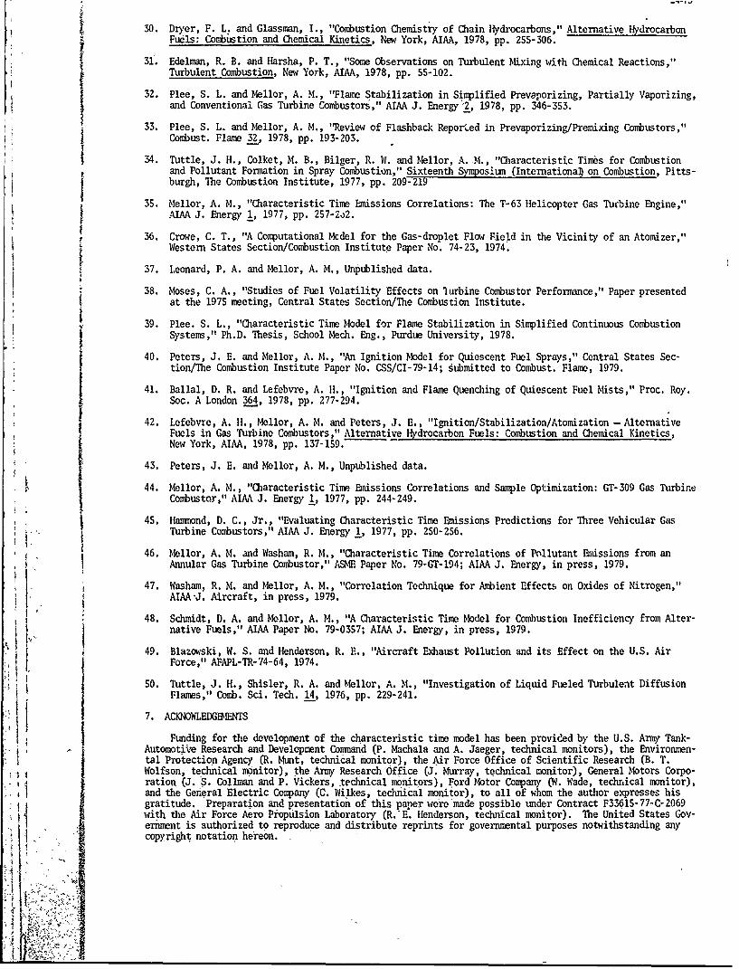
30. Dryer, F. L. and Glassman, I., "Combustion Chemistry of Chain Hydrocarbons," Alternative HydrocarbonFuels: Combustion and Chemical Kinetics, New York, AIMA, 1978, pp. 255-306.

31. Edelman, R. B. and Harsha, P. T., "Some Observations on Turbulent Mixing with Chemical Reactions,"Turbulent Combustion, New York, AIAA, 1978, pp. 55-102.

32. Plee, S. L. and Mellor, A. M., "Flame Stabilization in Simplified Prevaporizing, Partially Vaporizing,and Conventional Gas Turbine Combustors," AIAA J. Energy "2, 1978, pp. 346-353.

33. Plee, S. L. and Mellor, A. M., "Review of Flashback Repor',ed in Prevaporizing/Premixing Combustors,"Combust. Flame 32, 1978, pp. 193-203.

34. Tuttle, J. H., Colket, M. B., Bilger, R. W. and Mellor, A. M., "Characteristic Times for Combustionand Pollutant Formation in Spray Combustion," Sixteenth Symposiun (Internationa on Combustion, Pitts-burgh, The Combustion Institute, 1977, pp. 209-219

35. Mellor, A. M., "Characteristic Time Emissions Correlations: The T-63 Helicopter Gas Tutbine Engine,"AIAA J. Energy 1, 1977, pp. 257-2o2.

36. Crowe, C. T., "A Computational Mcdel for the Gas-droplet Flow Field in the Vicinity of an Atomizer,"Western States Section/Combustion Institute Paper No. 74-23, 1974.

37. Leonard, P. A. and Mellor, A. M., Unpublished data.

38. Moses, C. A., "Studios of Fuel Volatility Effects on turbine Combustor Performance," Paper presentedat the 1975 meeting, Central States Section/The Combustion Institute.

39. Plee. S. L., "Characteristic Time Model for Flame Stabilization in Simplified Continuous CombustionSystems," Ph.D. Thesis, School Mech. Eng., Purdue University, 1978.

40. Peters, J. E. and Mellor, A. M., "An Ignition Model for Quiescent Fuel Sprays," Central States Sec-tion/The Combustion Institute Paper No. CSS/CI-79-14; gubmitted to Combust. Flame, 1979.

41. Ballal, D. R. and Lefebvre, A. H., "Ignition and Flame Quenching of Quiescent Fuel Mists," Proc. Roy.Soc. A London 364, 1978, pp. 277-294.

42. Lefebvre, A. H., Mellor, A. M. and Peters, J. E., "Ignition/Stabilization/Atomization -AlternativeFuels in Gas Turbine Combustors," Alternative Hydrocarbon Fuels: Combustion and Chemical Kinetics,New York, AIAA, 1978, pp. 137-159.

43. Peters, J. E. and Mellor, A. M., Unpublished data.

44. Mellor, A. M., "Characteristic Time Emissions Correlations and Sample Opl:imization: GT-309 Gas TurbineCombustor," AIAA J. Energy 1, 1977, pp. 244-249.

45. Hammond, D. C., Jr., "Evaluating Characteristic Time Emissions Predictions for Three Vehicular GasTurbine Combustors," AIAA J. Energy 1, 1977, pp. 250-256.

46. Mellor, A. M. and Washam, R. M., "Characteristic Time Correlations of Pollutant Emissions from anAnnular Gas Turbine Combustor," qf&1E Paper No. 79-GT-194; AIAA J. Energy, in press, 1979.

47. Washam, R. M. and Mellor, A. M., "Correlation Technique for Ambient Effects on Oxides of Nitrogen,"AIAAJ. Aircraft, in press, 1979.

48. Schmidt, D. A. and Mellor, A. M., "A Characteristic Time Model for Combustion Inefficiency from Alter-native Fuels," AIAA Paper No. 79-0357; AIAA J. Energy, in press, 1979.

49. Blazowski, W. S. and Henderson, R. E., "Aircraft Exhaust Pollution and its Effect on the U.S. AirForce," AFAPL-TR-74-64, 1974.

50. Tuttle, J. H., Shisler, R. A. and Mellor, A. M., "Investigation of Liquid Fueled Turbulent DiffusionFlaws," Comb. Sci. Tech. 14, 1976, pp. 229-241.

F7. ACKNOWLED oTS

1Funding for the development of the characteristic time model has been provided by the U.S. Army Tank-Automot e Research and Development Command (P. Machala and A. Jaeger, technical monitors), the Environmen-tal Protection Agency (R, Munt, technical monitor), the Air Force Office of Scientific Research (B. T.Wolfson, technical monitor), the Army Research Office (J. Murray, technical monitor), General Motors Corpo-ration (J. S. Collman and P. Vickers, .technical monitors), Ford Motor Company (W. Wade, techical monitor),and the General Electric Company (C. Wilkes, technical monitor), to all of whom the author expresses hisgratitude. Preparation and presentation of this paper were made possible under Contract F33615-77-C-2069with the Air Force Aero Propuilsion Laboratory (R.'E. Henderson, technical monitor). The United States Gov-ernment is authorized to reproduce and distribute reprints for governmental purposes notwithstanding anycopyright notation hereon.

' •

COMBUSTION MODELLING WITHIN GAS TURBINE ENGINES,SOME APPLICATIONS AND LIMITATIONS.

J. Odgers.Universit6 LavalQuebec, Canada.

ABSTRACT

A review is given of some of the more pertinent models postulated to describe the perfermance of gasturbine combustors. Six different design/development stages are considered - (a) the initial sizing ofa combustor, (b) the initial development testing, (c) primary zone modelling, (d) secondary zone model-ling, (e) dilution zone modelling, (f) changes due to the alteration of ambient conditions. The modelsare assessed in scopel plausibility, experimentally, and in terms of time and economic justification.For (a) it is suggested that a zero-dimensional model will suffice, as also for (b). Item (c) willprobably require a three-dimensional model; (d) and (e) will probably suffice with a one - or two-dimen-sional model. For item (f) a zero-order model might well be satisfactory. If it can be produced withsufficient accuracy, a single complex (probably three-dimensional) model could adequately describe allitems, (a) to (f). A short discussion deals with the need of future data, and the paper recommnends thetype of models which may be used currently, and those which are likely to be used in the future.

1. INTRODUCTION.

It is about thirty years since the potential of gas turbine manufacture began to make itself felt asa major industry. Due to the high degree of technology, it immediately became obvious that the develop-ment of new combustion systems would be expensive and time consuming, Hence a search began for anunderstanding of the combustion processes so that modelling procedures could be instituted. Most of theearlier,parameters involved some form or other of Mach number scaling, since this involved most of thevariables of importance to performance. Further, Mach number correlated with the pressure drop acrossthe combustor, which in turn, was a function of the engine efficiency. Droplet evaporation characteristicswere also explored, but it was generally conceded that the droplets had but little overall effect providingthat the size was small (about 80 to 100 microns). Later, parameters were introduced based upon globalreactions within 'perfectly stirred reactors'(PSR's). An aspect, appreciated, but still very imperfectlyunderstood, is the very complex mixing process between air, fuel and products of reaction. The demandfor a long life engine has emphasised the need to better the knowledge of the heat transfer processeswithin the combustor and the-requirement for improved materials of construction.

As the years progressed, engineering 'know-how' enabled combustors to be made which operated withhigh combustion intensities, and in recent years it has been recognised that the combustion processesmight limit the combustor size-at some conditions, whereas previously aerodynamics were always assumed tobe the limiting factor. Simultaneously with the progress in engineering, the chemistry of flames hasbecome better known, and many of. the individual.rea.tions which comprise the process of the combustion ofhydrocarbons have been investigated,and their rate constants determined with fair accuracy. Recently,physicists have produced comprehensive mixing theories. Thus many of the individual bricks are nowavailable to produce a comprehensive model. It remains only to invent a technique to bind them together.The cement exists in the form of large computers which are capable of solving the complex equations.

the net result is that,whereas twenty years ago-the engineer had to 'make do' with elementary andlimited correlations, today he -is faced with a multitude of models ranging from simple zero-order ones tocomplex three-dimensional ones combining all-possible aspects of evaporation mixing and kinetic conside-rations, both with and without simultaneous heat tuansfer.

From an engineering viewpoint, the justification ofa model is, to a large measure, based upon -(a) Does it predict sufficlently accurately ?

u(b) How much time is needed to obtain a solution ?(c) How easy is it to understand the result, and what are

the possible implications ?

Cd) What is the financial cost of the solution ?

Generally (a) and (d) are the most important, but some of the proposed models are now so complex thatthe average~engineer has difficulty-in understanding-them, and very-rightly-he seeks an expert to act asconsultant. Unfortunately, -sometimes -the-consultant has a problem-in appreciating exactly what theengineer requires from the model. The net result is a certain amount of confusion whereby the reputationsof bothiengineer and consultan(or the mddel) ,may suffer.

J Therefore, what is needed is an appreciation-of the types of model available and their possible appli-4cation(s), the latter often depending upon the state of the development of the combustor. As an example-,

unless it was a perfect model, there would be little point to use a complex three-dimensional model forthe initial sizing-of.the.combustor, Such a-mddel would, however, be very appropriate to the specificationof the, primary,,zone-conditiois, and- their effects 'upon wall temperatures.

It is the intention of these notes to give some aid in this type of selection and to indicate, wherepossible, the known accuracy of the model suggested and its limitations.

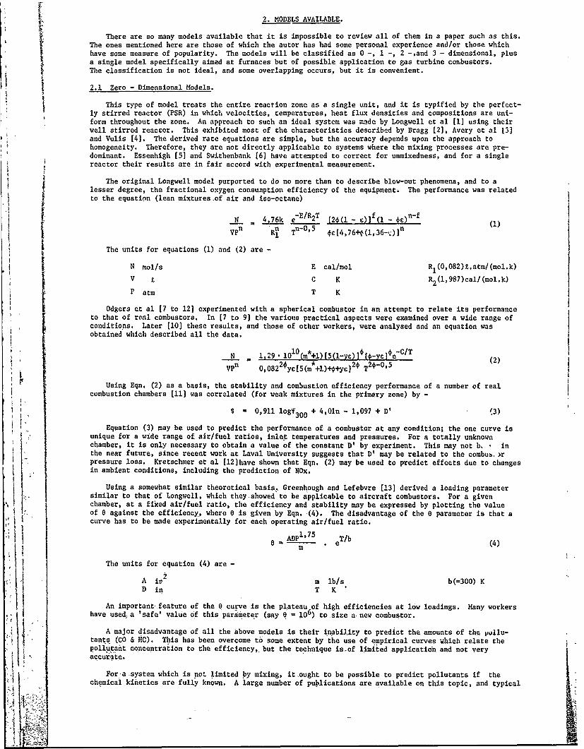
2. MODELS AVAILABLE.

There are so many models available that it is impossible to review all of them in a paper such as this.The ones mentioned here are those of which the autor has had some personal experience and/or those whichhave some measure of popularity. The models will be classified as 0 -, 1 -, 2 -,and 3 - dimensional, plusa single model specifically aimed at furnaces but of possible application to gas turbine combustors.The classification is not ideal, and some overlapping occurs, but it is convenient.

2.1 Zero - Dimensional Models.

This type of model treats the entire reaction zone as a single unit, and it is typified by the perfect-ly stirred reactor (PSR) in which velocities, temperatures, heat flux densities and compositions are uni-form throughout the zone. An approach to such an ideal system was made by Longwell et al [1] using theirwell stirred reactor. This exhibited most of the characteristics described by Bragg (2], Avery et al 13]and Vulis [4]. The derived rate equations are simple, but the accuracy depends upon the approach tohomogeneity. Therefore, they are not directly applicable to systems where the mixing processes are pre-dominant. Essenhigh [5] and Swithenbank [6] have attempted to correct for unmixedness, and for a singlereactor their results are in fair accord with experimental measurement.

The original Longwell model purported to do no more than to describe blow-out phenomena, and to alesser degree, the fractional oxygen consumption efficiency of the equipment; The performance was relatedto the equation (lean mixtures of air and iso-octane)

-E/R- f (I_,n-fN _ 4, 76k eE/R2T [2 (l - (1 -€) ()

VP Rl Tn -0 5 c(4,76+(1,36-)]-n

The units for equations (1) and (2) are -

N mol/s E cal/mol R (O,082)Z.atm/(mol.k)

V C K R2 (l,987)cal/(mol.k)

P atm T K

Odgers et al [7 to 12) experimented with a spherical combustor in an attempt to relate its performanceto that of real combustors. In [7 to 9] the various practical aspects were examined over a wide range ofconditions. Later [10] these results, and those of other workers, were analysed and an equation wasobtained which described all the data.

N _ 1,29. 1010(m*+l)[5(1-yc)l [0-y]eC/T (2)

VPn 0,0822 y[5(m,+l)+ +yc]2 T2 .0 ,5

Using Eqn, (2) as a basis, the stability and combustion efficiency performance of a number of realcombustion chambers [11] was correlated (for weak mixtures in the primary zone) by -

I - 0,911 logy300 + 4,Oln - 1,097 + D' 3)i300Equation (3) may be used to predict the performance of a combustor at any condition; the one curve is

unique for a wide range of air/fuel ratios, inlet temperatures and pressures. For a totally unknownchamber, it is only necessary to obtain a value of the constant D' by experiment. This may not b, . inthe near future, since recent work at Laval University suggests that D' may be related to the combub. )rpressure loss. Kretschmer et al [12]have shown that Eqn. (2) may be used to predict effects due to changesin ambient conditions, including the prediction of NOx.

Using a somewhat similar theoretical basis, Greenhough and Lefebvre [13] derived a loading parametersimilar to that of Longwell, which they showed to be applicable to aircraft combustors. For a givenchamber, at a fixed air/fuel ratio, the efficiency and stability may be expressed by plotting the value

of 0 against the efficiency, where 0 is given by Eqn. (4). The disadvantage of the 0 parameter is that acurve has to be made experimentally for each operating air/fuel ratio.

ADP1 7 5 T/b (4)

The units for equation (4) are -

A ivr m lb/s b(=300) KD in T K

An important feature of the 0 curve is the plateau of high efficiencies at 16w loadings. Many workershave used. a 'safe' value of this parameter (say q = l06) tosize anew combustor.1A major disadvantage of all the above models is their inability to predict the amounts of the illu-

tants (CO & HC). This has been overcome to some extent by the use of empirical curves which relate thepollutant concentration to the efficiency, but the technique isaof limited application and not veryaccurate.

For-a-system which is not limited by mixing, it~ought to be possible to predict pollutants if thechemical kinetics are fully known. A large number of publications are available on this topic, and typical

'Z

examples are given in [14 to 18). Generally the reaction is thought of as being a two-stage process,the breakdown of the hydrocarbon being followed by the combustion of the resultant carbon monoxide.The first reaction is fast compared with the second, and hence it is the kinetics of the CO burningthat limit the overall process and the amounts of pollutants produced. Reaction schemes have beenproposed ranging.from about 8 reactions to 40 or more. The number of reactions selected appears to bea function of the size of computer available. Models of this type have been used to predict the perfor-~mance of PSR's with fair success, but only over a limited range of conditions. As an example, Hammond

and Mellor [19] applied such a schemL to a reactor burning a propane/air mixture. They could only obtainviable solutions over the range 0 = 0,9 to 0 = 1,2, but witnin these limits theory and experiment agreedquite well. Similar schemes have been used by others (See review [20]) but the models appear to belimited in application and exhibit large errors when used to predict the performance of any of the other

systems.

2.2 One-Dimensional Models.

Although not so simple as the zero-divensional models, the one-dimensional models are still relat-ively simple and the calculations are cheap to do. Heat flux and species may be predicted, but a know-ledge of fluid flow and chemical heat release will then be required as input to the model. However, theuse of this concept enables one to depart from the PSR to one which is mixing limited, or reaction limited,or both (well-stirred reactor, WSR).

Typical of a simple reaction scheme is that of Essenhigh [5] which is applied to the atalysis of anadiabatic flame, using a PSR approach. The flume is divided into a series of cells, each of which isregarded as a PSR fed by the preceeding cell and feeding the succeeding one. The analysis yields a pairof algebraic equations, conveniently in finite difference form. The solution gives temperature orconcentration profiles as a function of distance or time, for the various input conditions. The theorygives a rational solution to the problem, but to date it has not been thoroughtly tested against practicalmeasurements.

Contrary to the above, Hottel et al [21] assume that combustion occurs so rapidly that the gas tem-perature at the burner end (of a furnace) is the adiabatic flame temperature. It is also assumed thatthe net radiative flux in the gas flow direction is negligible compared with that normal to it. Thus itis possible to predict the local flux density along the x-axis.

The module approach circumvents the requirement of a detailed analysis of the microstructure bybreaking the chamber into separate zones, each of which is assumed to behave in a predictable manner.In the short term, this kind of prediction may yield a much more valuable correlation than any of thetechniques previously discussed. Also, by a judicious choice of zones, modules may be selected whichwill represent, fairly accurately, a three-dimensional system.

Swithenbank [22] has attempted to model a turbojet combustor. The primary zone is represented bythree modules, a pair of WSR's coupled by a plug-flow reactor (PFR). The volumes are calculated fromjet entrainment theory, the total volume of the primary zone having been assessed previously by someinependent method. The volumes of the various reactors are estimated on the assumption of uniform gasdensity; the swirler and recirculation volumes are ratioed according to their mass flows; that of theprimary is considered to be symmetrical about the primary-orifices. The secondary zone has two modules,a WSR followed by a PFR. The voltme of the WSR is obtained by the assumption that .t is symmetricalabout the secondary zone holes, with its upstream boundary abutting the primary zone. The dilutionstirred reactor is supposed symmetrical about the dilution holes, and of a volume which is ratioed inproportion of its mass flow to that of the secondary zone, Between the secondary WSR and the dilutionWSR, the resultant volume is taken as being the secondary PFR. The plug flow module of the dilution zonei I is taken as that between the downstream end of the dilution WSR and the exit of the combustor. Thus, foreach module, the mass flow, volume and residence timehave been defined, and this may be used to predictthe composition leaving each module (providing there is a suftable reaction scheme). The output of onemodule becomes the input of the next, although within the primary zone an iterative calculation must beused since there is recirculation from one zone to another. Temperature traverses in a real combustorwere quite closely predicted using this model, but extensive testing has not been attempted.

So far, the models examined have assumed that the influence of fuel droplets is negligible. It isobvious that a more complete analysis could be made if the fuel droplet size and distribution were in-corporated together with evaporative effects' In this respect Mellor's proposal [23] is of some interest.The 'modules' are characterised by residence times, each time serving a particular region defined withinthe combustor. Mellor defines five such times - (i) the fuel drop lifetime, (ii) the eddy dissipationtime for the injected fluid (this represents small scale turbulent mixing near to the fuel injector inthe recirculation zone), (iii) the eddy dissipation time in the shear layer (this represents the largescale turbulent mixing of fresh air and the recirculated burned gas), (iv) the fuel ignition and burningi time (representing the time for homogeneous combustion of the fuel),and (v) the NO formation time. The

approach is very promising and could well yield very useful results, providing that the various residencetimes can be defined with.sufficient precision so that they may be used over a wide range of conditionsand geometries. To date,.not a grat deal of anlysis has bee'n experimentally investigated, but that whichhas is.apparently in fair agreem'ent with the predictions. NOx-and CO. exhaust-plane emissions have general-ly correlated well with their-respective time functions, except whenjfuel atomisation was poor. Theresults also confir ithe theory t ehogeneous combustion time and the ignition delay times aremuch shorter than either the droplet evaporationtimes or. the mixing times.

One dimensional models have proved-to be popular for theiprediction of NOx, largely due to the waythat the rai of f6rmation'dep endr so.ilargely upontemperature. Ad an example Heywood et al [24] tookthe secondary zone ofa c6mbustor and treated it as a one-dimensional model with instantaneous mixing ofthe secondary air. Calculated vaiues of W~x were about the same'value as those from aircraft engines.Hung [25 & 26] suggests a diffision limited model that predicts NOx within gas turbine combustors,

'1 including the use of nitrogen-containing fuels and the effects of water injection etc. The primary

zone is assumed to have a flow pattern similar to that described by Clarke [27], such that the threedimensional effect can be accounted for by the use of a quasi-one-dimensional model. For the swirler,the core radius of the reverse flow is determined in order to provide a boundary for the recirculationzone. Kollack and Aceto [28] studied the effects of recirculation in a combustor using a computer pro-

gramme which simultaneously solved the chemical kinetic, thermodynamic,and gas dynamic equations for apremixed one-dimensional recirculation system. The effect of hot gas recirculation was to form NOx atan earlier stage but to about the same maximum as the unr.:circulated case. Cold gas could reduce theNOx~by an order of magnitude.

2.3 Two-Dimensional Models.

These models predict with x-y coordinates and are suitable for systems (such as a gas-turbine com-bustor) where axi-symmetric flows prevail. The problem,is simplified if the flow is uni-directional andwithout recirculation, such as a simple, confined turbulent diffusion flame. The Patanker-Spaldingtechnique has been used to solve this problem [29;. The problem appears simple, but the flows are stillvery complex,and an adequate digital computer is required. Adequate modelling of the following featuresis required - (i) turbulence, (ii) reaction rate, (iii) radiation chemical kinetics (sometimes) and (iv),possible two-phase effects. The Genmix Computer Code is available to solve the problem, by which sixsimultaneous differential equations are solved for velocity, turbulence energy, turbulence scale,stagnation enthalpy, fuel concentration, and concentration fluctuations. Unfortunately, aircraft combus-tors exhibit recirculation, and this means that iterative procedures must be used instead of marchingintegration. For a relatively simple axi-symmetric furnace, computations of this kind have shown goodqualitative agreement with the experimentally determined features. A more complicated procedure isavailable for a system having pre-vapcurised fuel injected with swirling air into a film-co6led combustor(30]. The models employed for this scheme utilised turbulence, concentration fluctuations, radiation, asimple combustion kinetic scheme, and NOx kinetics. The computer code used was EASI (steady state model),and qualitative agreement was obtained with the experimental data. The difference was attributed in partto the fact that the combustor was only partially axi-symmetric. PLatt [31 & 32] has published a computerprogramme for the calculation of steady-flow, homogeneous reaction kinetics. It is implied that thiswould improve the Spalding-Gosman predictions withrespect to chemical kinetics. Recently, Spalding etal [33] have published predictions of the hydrodynamic and thermodynamic properties of flow relevant toa jet-engine after-burner. The flow was two-dimensional, axi-symmetric, unsteady, compressible, andchemically reacting. A fuel spray analysis was included. It is claimed that the numerical solutionprocedure gave a useful tool for investigating the 'buzz' in the engine after-burner.

2.4 Three-Dimensional Models.

These should be the 'all-can-do' models which,if sufficiently accurate,should yield perfect pre-dictions throughout the combustor. Currently, the known models predict species, concentrations, tem-peratures and velocities at any point within the combustor. It is possible to include the prediction offlame radiation and wall temperatures (with and without film cooling) at the price of a more complicated

i programme. The major problems preventing the general introduction of these models are -

(I) Assumptions involving flow and turbulence predictions may not be correct,

(ii) reaction kinetics may not be correct,(iii) factors governing carbon formation are not known, and this effects the accuracy of

flame radiation predictions,(iv) for accurate predictioni a large number of points is required (i.e. fine mesh). This

increases the computer time and cost,(v) a specialist engineer/pr6grammer is needed or else the work must be given to a consultant,(vi) a large computer must be available.

From this it might seem that the chance of a satisfatcory three-dimensional programme would be remote.However, considerable progress has been made and several models exist which demonstrate the correct trendsof conditions within the combustor. Perhaps the most comprehensive is that of Spalding [34]. This usesa finite difference computational procedure to predict quantitatively the local flow, heat transfer andcombustion processes inside a three-dimensional can combustor,where the flow is swirling and recircu-lating. A gaseous fuel system was employed. The process required the numerical solution of twelvesimultaneous differential equations in finite difference form. It is claimed that the system will com-pute economically and thereby substahtially reduce the experimental portion of the development time.Although the results given were not verified experimentally, it was noted that the physical models usedhad all been shown to be valid' in simpler two - and three - dimensional situations and that the procedurenow seemed to be ready to be employedwithin industry.

2.5 Miscellaneous Models.

Several models exist which do not readily fall into any of the above categories. Of the onesexamined, only oneseemed tobe of significance. This' modelwaq developed specifically for furnaces,but the results are so in'ereitiag that it would seemlogical to tdst the method against the performanceof a gas turbine. The model is that of Magnusse, et al [37], and it relates the rate of combustion tothe rate of eddy dissipation of turbulent eddies. The rate of reaction is expressed by the mean corscen-tration-of a~reacting specie, the turbulent kinetic energy and the rate Of dissipation of the turbutlentkinetic energy. Ii differs frdm'bther models ii that it does not call for prediction of fluctuations ofreacting species,and, additionally, it is applicable to both premixed and diffusion flames. A veryIi interesting feature is that the model can be used to predict soot formation and combustion in turbulentflames. The theory wAs t~sted'by-computlni the behaviour-of seven flames-represnting turbulent diffusionflames; premiked turbulent enclosed- flamee combined premiked/diffusion flames, and turbulent diffusionsooting-flames. In-all caseb close coirelation 'was obitaied be tween prediction and experiment.

k~i

-7,

2.6 Wall Cooling.

Most combustion models do not take wall cooling into account and those that do regard it as an

additional complication to an already complex model. Thus, only the two- and three-dimensional modelsof Spalding and co-workers attempt to make these predictions in conjunction with the combustor model.More generally, the combustor predictions are used to estimate the local gas conditions, and these arethen utilised with a separate film cooling correlation. A number of wall temperature prediction techniquesexist, [38 to 40] for example, which give reasonably satisfactory predictions. Basically, all of them usethe same equations, modified according to the whims of the user, and there seems little to chose in theaccuracy of predictions. These latter range from ± 20 to t 40K, depending upon conditions. The simplemodels appear to give about the same precision as the complex ones,

3. WHICH MODEL ? AND WHEN ?

One of the major problems,confronting anyone trying to assess the accuracy of a model, is that mostauthors justify their parameter solely against their own experimental work. Also, because of publicationdifficulties, the data are not usually given in sufficient detail to enable them to be used to check theparameters of other workers. Add to this that certain computer programmes are limited by propriety rights,

and the difficulties of comparing one model with another become obvious. To complicate the matterfurther, the economics of the calculation aresometimes a restricting factor, as is also the specialisedknowledge required to solve some of the more complex programmes. It is not, therefore, surprising thatthe following assessment must have reservations, and that no clear-cut picture will emerge.

The only models which have been tested at all comprehensively are the simple empirical and semi-empirical ones. An attempt will be made to indicate their accuracy, so that the proposers of futurecomplex models will have at least a target which they must surpass. This is not to denigrate the complexmodels from a scientific viewpoint, but the engineer must keep constantly in mind that his product mustbe economic; for the same accuracy, a cheap model is 'better' than a complex expensive one.

3.1 Initial Sizing of the Combustor.

A combustor has been selected which was developed to meet Condition 1, Table I, as its design point.To indicate what happens if a number of design conditions have to be met (instead of one), three new'design .onditions have been added.

TABLE I.

Cond. ma T2 P 2 tP/P ve mf pz

kg/s K 105 Pa kg/s

1* 4,67 476 4,05 0,05 0,056 0,0778 1,02 10,06 641 10,13 0,05 0,056 , 0,1677 1,03 17,97 803 20,26 -0,05 0,056 0,2295 1,04 0,74 300 1,01 0,0125 0,028 0,0082 0,67

* Original design point.

Five different (all simple)-correlation parameters have been selected to~determine the size, basedupon either aerodynamic or combustion performance characteristics. The relationships are well known,but they have been rearranged in SI'units.

(I) Mach NumberL'Relationship. [35]

m rTma 14,3 A P (5)

(ii) Pressure Loss Relationship. (36]

A - 5 9 ,a- P -- (6)

(iii) Bragg's Relationship. [41]

A =0,01621 - 05(7)1

(iv) ThetatParameter. [13] (=99%)Ab=1,88,10 e T/b(8

(v) Odgers-Carrier. Parameter. [11] (=99%),

d 3745 0,411 0,3333745,(300/T) (mf (9)

This latter parameter is specific to 0 = 1,0 in the primary zone. For any other value of 0, Eqn. (3)

must be used.

4_

It is important to realise that at least two of the above parameters must be used (one aerodynamicand one combustion). In the Laval Laboratories all five are employed. The results given by the aboveequations, for the conditions of Table I, are given in, Table II. It is interesting that both Eqns. (8 &9) predict the need for-.a larger chamber to meet the combustion efficiency of 99% implicit in the valuesselected for these-equations. In fact, if the final real chamber dimensions are inserted into the orig-inal version of Eqn. (9) (i~e. Eqn. 3), then for- condition 4, the predicted efficiency of 93% is in fairaccord with the measured value of 91%. The results of Table II clearly demonstrate the need tc considerall the running points as design points.- The days of designing to tacat a single 'critical' conditionare past. The demand of very high combustion efficiencies at idling ronditions (to meet environmentalrequirements) requires a very critical look at the initial sizing prozedure.

TABLE II

Cond. Eqn. 5* 6 7 8 9No. No.

Value

1 A mn2 0,0642 0,0662 0,0308 0,0843 0,0713D m 0,286 0,290 0,198 0,328 0,301d M 0,228 0,232 0,139 0,262 0,241

A m 0,0642 0,0662 0,0308 0,0483 0,0274D m 0,286 0,290 0,198 0,206 0,187d m 0,228 0,232 0,139 0,165 0,150

3 A m2 0,0642 0,0662 0,0308 0,0153 0,0274D m 0,286 0,290 0,198 0,140 0,130d m 0,228 0,232 0,139 0,112 0,104

A m 0,0642 0,0662 N/A 0,0943 0,172#D m 0,286 0,290 0,347 0,468#d m 0,227 0,232 0,277 0,374#

* This is the actual size of the combusetor which was based upon a casing Mach number-0,056.

# 'Idling' conditions based upon Eqn. (3).

3.2 Initial Combustor Development.

It does not come within the province of this paper to discuss flow visualisation experiments andtheir value to the engineer, -but itis assumed that these studies will have been carried out and that

S-the results would, have indicated that (a)-the flowpattern was-satisfactory, (b).the film cooling jetsf appear satisfactory, (c) jet penetration& into the various zones are satisfactory,and (d) the primary

and recirculation zone volumes are well defined. the combustor pressure loss will also have been measuredand found satisfactory.

Following this, atmospheric testing will be done to verify the.combustor performance at ground leveland to forecast its.performance-at other conditions. The ideal model would-predict ignitability, combus-tion efficiency, exhaust traverse quality, type and quantity of pollutants, and blow-out characteristics.An indication that the flame-tube wall temperatures are satisfactory would also be useful. All thiscould be done with a satisfactory three-dimensional model, but at present no~proven one exists which isboth accurate and cheap. How accurate must it be? Obviously combustion efficiencies must eventuallypredict to better than 1%; the other topics are less critical providing that the operating characteristicsare superior to those demanded. They should at least be-better than the simple models cited below.

Equation (3) may be used to predict combustion efficienciesat all conditions providing that theconstant D' has been first established. Theoretically only a single efficiency determination is neededto establish D'. In practice the mean of four determinations provides a much more reliable figure. At

least two measurements should be made of efficiences in excess of 99%, and at least one of the order of90%. The efficiencies need to be accurate and demand the use-ofgasanalysis; pyroptilid Leshniques aresimply not accurate enough.

For the following example, a combustor was run at atfiospheric pressure but at four different condi-tions. The value of-D' was'assessed at 0,336. The combustor ias then run oyera~wide range of conditions(A/F 216 to 34, P2 0,34 to 7,66 atm, T- 243 to 545Kj. Thepredicied and measured efficiencies areindicated in Fig. (1). It is'obvious hat the gan analysis res"u1ts agree with the predictions betterthan do the pyrometric Values. Earlier analysis[11] indicato that the latter could have errors of t5%.More recent work suggests that Eqn. (3) will predict within, Z 2% at low efficiencies (say 80 to 90%) andbetter than 1% at high efficiencies (say'99%). Eqn. (3)mo aleo b used to indicate the blow-out curvefor a combustor. For a PSR flame extinction seems to-oc-:' at a relativqly constant flame temperature,of the order-of 1500K. In a real combustor due. to mi)i'igac' droplet evaporation, the temperature issomewhat lower. Equation (3) has a very steep fall ofttoward n 0, at an efficiency of 60%. Thisvalue of n may- be inserted into Eqn. (3) And asiumdd m-give blow-out loadings.

0, Figure 2 compares'the predictions with experimentalresults. As a 'general indication the prediction is

- - - - satisfactory, but there is considerable room forimprovement. To the best knowledge of the author,

S:no prediction technique exists which will predict

0 AT ignition limits. Of course, if the system was per-0,1 - * fect, the ignition and stability limits would coin-

TV ~ cide. For the particular can used here, a roughapproximatiop to the ignition limits was achieved

Aq) *. by putting n = 90% in Eqn. (3). This could well be0 •circumstantial.

A k •An alternative to the use of Eqn. (3) is toA. use the 0 correlation (Eqn. 4). This, however,

:A 0.0 •requires more experiments, since three or four points

* S * 0 . are required to establish each curve for a single

A I0 operat4ng air/fuel ratio. Typical results, for theS- - same chamber as above, are shown in Figs. 3 and 4.

-01 * The A/F - 60/1 points show mi.ch less scatter thanthose for A/F = 100/1. This might be indicative of

-the need to assume a variable reaction order, asper Eqn. (3). As before, the fall-off in efficiencymay be used to predict blow-out. The accuracy ofprediction is about the same as that given by Eqn.3.

0,7 0,8 0,9 1gmeasured Both of the above techniques predict efficiency

at the exhaust. If pollutants are required, eitheran alternative parameter must be sought, or some

4. Points used to define D'. estimate may be made by assuming that the ratio ofE Efficiencies determined by gas analysis. CO to HC varies in the same way as the measured

Efficiencies determined by pyrometry. values used to define the correlation equation. IfAthe combustion efficiency is in excess of 99,5%,n ffi n measured -n predicted, the exercise becomes academic. For the prediction

SFig. 1. Prediction of Combustion Efficiencies of NOx, the curve of Kretschmer [12] may be used,F or that of Lipfert [42] or most other simple corre-

Using Equation (3). lations.

3 1Eqn. (,.0,6) An indication as to the film cooling may be

*• Experiment obtained from the following equation (empirical)developed at Laval University.

- %Flm Cooling - 0,1 Ti - 30 (t10%) (10)

. IT T*e : An equation which predicts (very approximately)z * : \O.4 the traverse quality is -

Q © (73,85 - 138,5 AP/P) - 27L/d (11)

max mean (lla)Q Mean TempRise

Both Eqns. (10 & 11) are relevant to convention-1 i"_ _ al combustors with conventional fuel systems. There

are indications that neither apply (for instance)00 2 to air-blast fuel injection systems. The accuracy

mfIVP" .bIs ft3atmn of prediction for both equations is not srtisfactory,fI and better correlations should be sought. They are

Fig. 2. Prediction of Blow-out Using Eqn. (3) only a guide, and should be accepted as such.

1

0.8 01.8.0,70

7/•0,_6I 4 1 0,6 ?,1F 0 1

A0

A/F , 1 0,5 .....-,/* AF 100/1

2Xt0 4 106 21004 e0s O 106

Fig. 3 Prediction of Efficiency,Theta Parameter. Fig.4 Prediction of Efficiency,Theta Parameter.I ,AI

It is bbvious that there is room for improvement for all the above techniques. They are given here(a) because they are 'better than nothing', and (b) they give-an idea of the accuracy which must bebettered by any replacement correlations. Assuming that the combustor design has proved to be satisfact-ory at this stage, the next phase is to examine the performance of the individual zones of the combustor.

3.3 Primary Zone Model.

'Any model for use in- the primary zone should predict one or more of the following -

(i) flame temperature distribution.(ii) flame emissivity.(iii) local air/fuel and composition.(iv) local gas velocities.(v) combustor wall temperatures.(Vi) flame stability.(vii) carbon formation and consumption.

There are no simple models which will predict accurately within this zone. Crude, empirical modelsexist which give some idea of the mean gas temperature and emissivity, hot gas velocity and cooling jetvelocity. Thus, an appraisal of the wall temperature can be made which, strangely enough,. is often suf-ficiently accurate for engineering purposes. Again, these predictions, and the observed accuracy, re-present a target for the more refined techniques.

For the sole purpose of wall temperature prediction, the following empirical equations have beendeveloped at Laval University. They relate to the various mean hot gas temperatures.

Tr T, T - (12)a0

r= 0,56 + 0,44 tanh [1,5475 x 10 -3(T + 1081nPa - 1863)] (12a)

T - T + 0,5n (AT - 1,0 + AT) (13)pz a pz pz

- 0,71 + 0,29 tanh (1,5475 x 10-T3 + 108ZnP - 1363)] (13a)

Toutpz = Ta + lpz ATpz (14)

The high values ascribed to these equations are excused by the importance of flame radiation in thezone. Based upon the experimental information available it is estimated that the flame temperaturespredicted in this way have the following accuracy -

+ lOOK at conditions of low efficiency+ 50K at conditions of high efficiency

The heat transfer equations used to calculate the wall temperature are due to tefebvre et al [13]-

-e1,5 [T2,5 _2 , 5 .R1 w eg T g (15)

I J'I A0 8 dO c wRI 0, [ T Y (17)C2 0,8

C 0,02L m l - T] (18)

K 04 - 4 (19)

12 N2 C

.I ¢ RZ + C 1 = R2 +C2 =K

I2 (20)

The emissivity equation is also that of Lefebvre -

eg = 1 - exp. [..0,286p Lu(f 1)0 ;5. T;1 ' 5 ] (2]:)

However, the luminosity equation~has been d -rvd nti lbd~try, based upon the data given in

The ifilm cooling Kxrsin~sta ifOgr n hie [46]8)'

- ('F=.A 0,8 0,C -2 ; 0,02' Tg 08 n, IT- TC a f (18)c

Using the above equations and the appropriate film cooling correlation (depenain,; upon the geometryof the film cooling device), the wall temperatures may be predicted in the primary zone with an accuracyof not less than + 50K. A typical result is given in Fig. 5. The above accuracy cannot be guaranteedfor aik-blast or similar systems.

In order to provide the necessary detail, the14 complexity of the primary zone demands a two - or

Experimental a three-dimensional model. Those of Spalding and

2 'Scatter Co. are of considerable interest, as also that ofS10[37]. It seems very doubtful that any of the modular

techniques would give the required structural detail.It would be of considerable interest to compare someof these models and their corresponding predictions.Ma It should now be possible to provide the experimen-tal data required to fully test such techniques.

12 Gas analysis methods now exist which will providethe required composition data, and the Pulse Thermo-couple developed by Kretschmer has been shown to be

&Predictions an accurate and fast way of evaluating the tempera-_ _ _ture distribution [47]. A typical set of traverse

10 20. 30 40 data through an aircraft combustor is shown in Fig.6.2 bar The values were obtainedrby sampling through the air2admission holes; sampies between holes show a some-

what different pattern. The temperatures measured7ig. 5 Wall Temperature Predictions. agree closely whith those given by detailed gas

analyses, although the latter show the fuel efficien-21' cy to~be quite low. Indications are that the fuel

0-!-0 PZ efficiency in the primary zone is of the ordcr ofc *em SZ 50%. These results support the assumption that

T ii- DZ hydrocarbons are the result of mixing inefficiencyX10-2 Iand the remaining species are kinetic limited. It

K has been shown[48]that even complety premixed airand fuel yield considerable amounts of hydrocarbons

.I k , would cause considerable difficulty to the 'mixing

15*', | 1 limited' enthusiasts.

15: ! ' 1 3.4 Secondary Zone Model.

bly forecast This is the region where the combustion is sensi-C bly completed and the model should forecast-

9* 3 Cli M~ i gas temperature distribution0Ii ii) local A/F and species distribution. 1(ii) gas velocity distribution. V I(iv) wall temperature distribution.

0 A The flows in this zone are still complex, and it* is suggested that the same models be used in this

region as for the primary zone. A few gas analysismeasurements suggest that Eqn. (3) will reasonably

Spredict the efficiency at the exit of this zone.3] 9, Other than this', the only model used extensively is

3 one to predict wall temperatures. This is identical0 r in procedure to that outlined in Para. 3.3, except

that the mean gas temperatures are estimated (at

Fig. 6 Zoae Temperatures in an Aircraft Combustor. Laval) by the following empirical equations.

sz pz (24)

T=Tout+nA,T°Utsz T2 + AT- z (25)

Tmean - Tin + Tout

2 (26)

The simple model predicts wall temperatures with an accuracy of + 30K.

3.5 Dilution Zone Model.

For the simple-model to predict the wall temperatures, the ptocedure is as before but with gas tem-peratures given by -

Tin, =ToutTnzfi°Usz (27)Toutd f T2 + n Al

dz 2 dz (28)

Tmeandz = Tin + ToutT c c a -(29)

, '!: . The accuracy is again 30K.

Obviously the complex model used to predict conditions in the primary and secondary zones could

also be used for this zone. However, if it can be definetely established that combustion is sensibly

completed within the secondary zone, then the possibility of a much simpler model is obvious.

3.6 Changes in Ambient Conditions.

If it can be avoided, there seems to be little point in using a complex model for this purpose.

The problem is simplyfied to some extent by the fact that the performance of the combustor is already

known at some 'near' condition. Hence, it is usually possible to utilise sometype of 'scaling factor'Kretschmer [12] suggests several such. An example of the predicted and measured changes in efficiency,due to increased inlet temperature, is given in Fig. 7. The agreement is satisfactory, but the methodgives no indication of the contribution of the individual pollutants. These have to be assessed froma prior knowledge of the combustor characteristics at other conditions.

Kretschmer's techniques will also predict NOx0 ,changes fairly accurately. Marzeski et al (49]I /specifically examine the effects of ambient changes

0,97 upon emissions at idling conditions. They give for-;! / mulae for changes in HC and NOx, but report a failure

0,969 when attempting the prediction of CO. There seemsto be a possibility of using this work in conjunction

0,968- - with that of [12] in order to obtain a full range ofpredictions at all conditions.

0,961 - 3.7 Prediction of Oxides of Nitrogen.

0,966 NOx has assumed such a significance in the fieldof pollution that it seems reasonable to consider mo-

0, ____I ,____I__ I __L___ ,1, dels specific to its prediction. The published lite-

300 305 310 K 315 rature is so enormous that a full review here is notAmbient Temperature possible. Comment will be reserved to those papers

which, in the author's opinion, have widespread appli-cation. For approximate estimates, the correlations

Fig.7 Effects of Ambient Temperature upon of Kretschmer [12] and Lippferv [50] are adequate.Combustion Efficiency. The model of Hung [25 & 26] is more sophisticated

and is claimed to predict accurately the effects of(a) combustor conditions (b) steam and water injection (c) the presence of nitrogen in the fuels (d)ambient changes and (e) changes in combustor geomotry. The claims are supported by experimental evidence,and the technique is worthy of further consideration.

4. DISCUSSION

It must be concluded that there is no model available which will satisfactorily take into accountall the variables which occur in the operation of gas turbine combustors and predict the performance withsufficient accuracy. A number of models exist of limited tpplication, and othersome encourage furtherinvestigation since they have the prospect of more general usage, Whilst work to date has shed light onthe general understanding of the combustion processes, the situation is that there is still no modelcap'ble of catering for the predictive requirements of real combustors.

A major reason for this is the absence of accurate experimental data within the combustors whichwould enable any theory to be comprehensively tested. What is required (say) is meaaured data from fivecombustors operated over a range of conditions. For each combustor there would be a 'map' of the primary,secondary and dilution zones giving detailed distributions of (a) temperature (b) species (c) gas emissi-vity (d) velocities (e) fuel droplet sizes and placement (f) carbon measurements and (g) wall temperaturemeasurements. The chambers should be selected so as to include geometry variations, conventional fuelinjection, air-blast injection, pre-vapourised fuel and premixed fuel/air.

i It is realised that this would be an expensive project, but the end-result would be to possess aset of data sufficient to test any proposed theory. The desire for an adequate model is now so strong

that it ought to be possible to set up a national, or even an international, committee to standardisethe techniques of measurement, obtain the necessary funds and to place the work in approved laboratories.If the results led to a satisfactory 'universal' modeli the sayings in development time would more thanamply repay the cost of the work, as well a's assisting in the understanding of the complex phenomema ofcombustion within a real system. It is further believed that any model developed for the gas turbinecombustce could have widespread application to other continuous flow combustion systems such as furnacesand domestic heating equipment.

NOMENCLATURE

2A Outer casing reference area ma Flame tube reference area mb Constant depending upon A/F (see 13)

=E/R K

' D Outer casing reference diameter mD' Constantd Flame tube reference diameter mE Activation energy J/mole Emissivityf Reaction order for fuelf Fuel/air ratio (by mass) Eqfi. (21)K Constant

NOMENCLATURE (Cont'd)

k Any constantL Length of dilution zone m

Lu Flame luminosityMa Mach numberm mass flow mol/s

m* Ratio mols inerts/mols oxygenN Mass flow molls

n Ovterall reaction orderO/F Oxygen/fuel ratio (mass or volume)P Pressure Pa (atm)Q Traverse qualityq Velocity head PaR Gas constant -Jimql 4 K)S Radiation constant (5,667 x 10 8 ) WAmK )

s Slot thickness mT Temperature TV Volume m (1)x Distance from film cooling slot mAP Pressure drop PaAT Theoretical temperature rise K

C Fractional oxygen consumption efficiencye Parameter, see:Eqn. (4)X Gas conductivity WAm.K)

Gas viscosity kg/sm Pj.sy Fuel loading, see Eqn. (3), Ref. 11 kg/ (s.m Pan)r Combustion efficiencyI Parameter = log log (1/n)

a Engine Compression Ratio SUFFIXES

a inlet air (or amount of air in outer casing at any point.c film coolingdz dilution zonef fuelg hot gas or flame gasi at inlet conditionsm masspz primary zoner recirculation zoneref reference pointsz secondary zonev volumew wallI refered to within combustor2 refered to outer casing

REFERENCES

1. Longell, J.P. & Weiss, M.A., "High Temperature Reaction Rates in Hydrocarbon Combustion", I. & E.C.,!" 47, No. 8, p. 1634.

2. Bragg, S.L., British Aeronautical Research Council, "Application of Reaction Rate Theory to Combus-tion Chamber Analysis", 1953, Paper No. 16170.

3. Avery, W.H. & Hart, R.W., "Combustor Performance with Instantaneous Mixing", I. & E.C., 45, No. 8,1953, p. 1634.

4. Vulis, L.A., "Thermal Regions in Combustion", New York, Mc Graw Hill, 1961.

5. Essenhigh, R., "An Introduction to Stirred Reactor Theory Applied to Design of Com'ustors, Combus-tion Te':hnology", Pennsylvania, State University, Some Modern Developments, 1973.

6. Swithenbank, J., Poll, I. & Vincent, M.W., "Combustion-Design Fundamentals", 14th Symposium (Int.)

on Coinbusiion, Combustion Institute, 1973, p. 627.

7. Clarke, A.E., et al, "Combustion Stability in a-Spherical Combustor", 7th Symposium (Int.) on Com-bustions Butterworth, 1959, p.664 .

8. Clirke, 2AiE., et 61, "Further Studies of Combustion Phenomena in a Spherical Combustor", 8th Sympo-sium (Int.) on Combustion, Williams'& Wilkins, 1962, p.,-982.

9. Clarke, A.E., et al, "Combustion Processes in a Spherica. Combustor", 10th Symposium (Int.) on Com-

bustion, Combustion Institute, 1965, p, 1151.

10. Kretschmer, D. & Odgers, J., "Modelling of Gas Turbine Combustors - A Convenient Reaction Rate

Equatior.", ASME, J . Eng. for Power, July 1972; p. 173.

REFERENCES (Cont'd)

11. Odgers, J. & Carrier, C., "Modelling of Gas Turbine Combustors - Consideration of CombustionEfficiency and Stability", Trans. ASME, J. Eng. Power, April 1973, pp. 105-113.

12. Kretschmer, D. & Odgers, J., "Modelling of Combustors - The Effects of Ambient Conditions UponPerformance", ASME, Paper No. 73-WA/GT-6, 1973.

13. Lefebvre, A.H. & Greenhough, V.W., "Some Applications of Combustion Theory to Gas Turbine Develop-ment", 6th Symposium (Int.) on Combustion, Reinhold Publishing Corp., 1957, p. 858.

14. Osgerby, I. T., "Literature Review of Turbine Combustion Modelling and Emissions", AIAA Journal,Vol. 12, No. 6, June 1974, pp. 743-754.

15. Edelman, R. & Economos, C., "A Mathematical Model for Jet Engine Combustor Pollutant Emissions",AIAA/SAE, 7th Propulsion Joint Specialist Conference, Paper No. 71-714, June 1971.

16. D'Souza, M.V. & Karim, G.A., "An Analytical Study of Methane Oxidation in a Steady - Flow Reactor",Comb. Science & Tech., 3, 1971, p. 83.

17. Edelman, R.B. & Fortune, 0., "A Quasi-Global Chemical Kinetic Model for the Finite Rate Combustion

of Hydrocarbon Fuels", AIAA, Paper 69-86, 1969.

18. Kennedy, L..A., "Modelling of Combustion Chambers for Predicting Pollutant Concentrations", ASME,Paper No. 74-HT-NN, 1973.

19. Hammond Jr., D.C. & Mellor, A.M., "Analytical Calculations for the Performance and PollutantEmissions of the Gas Turbine Combustors", revised version of AIAA, Paper No. 71-711, Comb. ScienceTech., 4, 1971, p. 101.

20. Odgers, J., "Current Theories of Combustion within Gas Turbine Chambers", 15th Symposium (Int.) onCombustion, Combustion Institute, 1974, p.1 321 .

21, Hottel, H.C., "Radiative Transfer", Me Graw Hill, 1967.

22. Swithenbank, J., Poll, I. & Vincent, M.W., "Combustion Design Fundamentals", 14th Symposium (Int.)on Combustion, Combustion Institute, 1973, p. 627.

23. Mellor, A.M., Bilger, R.W., Shisler, R.A. & Tuttle, J.H., "Emissions from Aircraft Fuel Nozzle Flames",Report No. PURDU-CL-75-04, July 1975.

24. Heywood, J. B., "Gas Turbine Combustor Modelling for Calculating Nitric Oxide Emissions", AIAA, PaperNo. 71-7112, 1971.

25. Hung, W.S.Y., "An Experimentally Verified NOx Emission MIodel fo, Gas Turbine Combustors", ASME, Pa-

per No. 75-GT-71, 1975.

26. Hung, W.S.Y., "A Diffusion Limited Model that Accurately Predicts the NOx Emissions from Gas TurbineCombustors Including the Use of Nitrogen Containing Fuels", ASME, Paper No. 75-Pwr-l1, Nov. 1975.

27. Clarke, J.S., "The Relation of Specific Heat Release to Pressure Drop in Aero-Gas-Turbine CombustionChambers", Proc. IME-ASME, Conf. on Coxtbustion, 1955, p. 354.

28. Kollrack, R. & Aceto, L.D., "Recirculation Effects in Gas Turbine Combustors", 95th Winter AnnualMeeting of the ASME, Paper No. 74-WA/FT-3, Nov. 18, 1974.

29. Patan ,ar, S.V., "Heat and Mass Transfer in Boundary Layers", London Intertext Books, 1970.

30. SpAdfoSg, D.B., "Numerical Computation of Fractical Combustion Chamber-Flows", AGARD-CP-164, PaperNo. 1-1, 1974, p. II-1.

31. Pra-tt, D.T., Washington StateUniversity, Dep. Mech. Eng., "PSR-A Computer Prograrn for Calculationof Steady Flow homogeneous Combustion Reaction Kinetics", 1974, Bulletin 336.

32. Pratt, D.T., "Mixing and Chemical Reaction in Continuous Combustion", Prog. Eng, Combust. Sc. Vol. I,1976, p. 1.

33. Spalding, D.B., Pratt, D.T., Elgobashi, S. & Srivatsa, S.K., "Unsteady Combustion of Fuel Spray inJet-Engine Afterburaers", ISABE, Munich, March 1976, p. 447.

34. Spalding, D.B. & Serag-Eldin, M.A., "Prediction of the Flow and Combustion Processes in a Three-Dimensional Combustion Chamber", ISABE,Munich, farch,1976, 489.

35'. Lewitt, E.H., "Hydraulics", Pitman, 1923.

36. Rouse, H., "Elementary Mechanics of Fluids, Wiley, 1946.

37. Magnussen, B.F., "On Mathematical Modelling of Turbulent Combustion with Special Emphais on SootFormation and Combustion", 16th Symposium (Int.) on Combustion, 1976.

REFERENCES (Cont id)

38. Spalding, D.B., " Prediction of Adiabatic Wall Temperatures in Film Cooling Systems", AIAA Journal,Vol. 3, No. 5, May i965, p. 966.

39. Sturgess, J., "Correlation of Data and Prediction of Effectiveness from Film Cooling Geometries ofa Practical Nature", Cranfield Int'II Prop. Symposium, 1969.

40. Papell, S.S. & Trout, A.M., "Experimental Investigation of Air Film Cooling Applied to an AdiabaticWall by Means of an Axially Discharging Slot", NASA, Tech. Note D-9.

41. Bragg, S.L., Paper to the Combustion and Fuels Committee of the ARC, "Application of ReactionRate

Theory to Combustion Chamber Analysis", Sept. 1953.

42. Lipfert, F.W., "Correlation of Gas Turbine Emission Data", ASME, Paper No. 72-GT-60 1972.

43. Lefebvre, A.H. & Herbert, M.V., "Heat Transfer Processes in Gas Turbine Combustion Chambers",Proceedings of the Institute of Mechanical Engineers, Vol. 174, No. 12, 1960, p. 463.

44. Marsland, J., Odgers, J. & Winter, J., "The Effects of Flame Radiation on Flame-Tube.Metal Tempera-tures", 12th Symposium (Tnt.) on Combustion, Combustion Institute, 1969, pp. 1265-1276.

45. Lefebvre, A.H. & Herbert, M.V., "Heat Transfer Processes in Gas Turbine Combustion Chambers",Proceedings of the Institute of Mechanical Engineers, Vol. 174, No. 12, 1960, p. 463.

46. Odgers, J., "Lucas Gas Turbine", Nov. 1963, Rep. No. B48314, (Unpublished Work).

47. Kretschmer, D., Odgers, J. & Schlader, A.F., "The Pulsed Thermocouple for Gas Turbine Application",ASME, Paper No. 76-GT-l, April 1976.

48. Roy, P., Schalder, A.F. & Odgers, J., "Premixed Combustion ii. a Baffle Combustor and the Effect ofSteam Injection", ASME, Paper No. 74-GT-8, 1974.

49. Marzeski, J.W. & Blazowki, W.S., "Ambient Temperature and Pressure Corrections for Aircraft GasTurbine Idle Pollutant Emissions", ASME, Paper No. 76-GT-130, 1976.

50. Lipfert, F.W., "Correlation of Gas Turbine Emission Data", ASME Paper No. 72-GT-60,1972.

-i-

DISCUSSION

W.Krockow, GeAs you referred to my paper, comparing your temperature distribution with the presented AFR distribution in mypaper, I must point out, that this comparison is invalid because I made a statistical distribution while you presenteda local distribution. You can do a comparison if you plot the mass fraction of equal temperature containing areasabove temperature.

Author's ReplyI thank Dr Krockow fnr his correction and will examine our data in the light of his remark. My point was that itseems unlikely that all flame tube geometries could be represented by the same distribution.

D.C.Dryburgh, UKI should like to comment on Prof. (Cdgers talk and say a word in defence of large models.

(1) We are having to consider much more complex flame tubes and we never know with models whether thecorrelations are still valid.

(2) I agree with Prof. Odgers that it is probably unlikely that any single model will do everything.

(3) Models have an important role in giving improved understanding of what is going on in the flame tube. We haveused a 3-D model to look on the complex 3D flow near a swirl injector in an annular flame tube and the flow isvery complex and impossible to gvess. The details are needed by the combustion engineer developing theflame tube. Having got to this stage it is worth while extending the model to calculate the chemistry and theefficiency.

Author's ReplyWith regard to the first point, I agree that it is unwise to use simple models outside the range of conditions for whichthey were established but my experience with several larger models is that they appear even more sensitive to extra-polation.

The third item is well put. I had hoped that during my presentation that I had expressed that the complex modeldoes indeed describe phenomena which is beyond the scop& of the simple model. However, this does not alter mybelief that, currently, the simple model offers more to the design engineer and will do so for some time to come.

D.T.Pratt, USRemember those 2 famous words:

(1) Enrico Fermi (on the 20th anniversary of quantum mechanics): "We are still confused, but on a higher level".

(2) Another quote: "Garbage in, Garbage out" holds as well for slide rules as for computers!

Author's ReplyIt is difficult to make a response to these quotationb except to say that I could not help but agree with them asstatements.

' tComment by D.T.Prtt, US,n context (p.25-4, § 2.3), Reference 31 and 32 should be:

31. Pratt, D.T. Calculation of Chemically Reacti, .I Flows with Complex Chemistry, in Studies inConvection, Vol,2, B.E.Launder, Ed., Academic Press, 1977.

32. Pratt, D.T. CREK-A Computer Program fir Calculation of Combustion Reaction EquilibriumWorneck, J.J. and Kinetics in Laminar or Turbulent Flows - Washington State University Report

WSU-ME-TEL,76-1, 1976.

S.Wittig, Ge"Accuracy" as defined seems not always to have highest priority in this phase of modelling. Even in the relatively

, simple case (see 3.5) of the dilution zone, simple correlations will be insufficient in really understanding the effectsof various praneters. The need for more advanced detailed models in aiding the designer seems to be clearly-established.

Autior's ReplyAs I said in my presentation, the accuracy of the simple models is not yet sufficient,-but it seems to be often better

than the complex m odels. Phenonenologically, the latter produce a better description but it is my impression thatin the immediate future tile combustion engineer will have to rely oi, empirical or semi-empirical models. I do notsee the complex models being available (with sufficient quantitative accuiacy) within the next five to ten years.

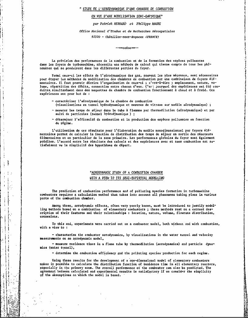
ETUE DE L' AERODYNAAM1QUE V' NE CHAMBRE DE COMBUSTION

EN VUE V'UNE MODELISATION SEMI-EMPIRIQUE"

par Patrick REBRARD et Philippe MAGRE

Office National d'Etudcs et de Recheiches MrospatiaZesH92320 - Ch~tillon-SOUS-Bagneux (FRANCE)

La prdvisi.on des performances de la combustion et de la formation des espaces polluantesdans lea foyers de turbomachine, nficessite une m~thode de calcul qui tienne compte de tous lea ph6-nomanes qui se produisent dana les diff~rentes parties du foyer.

Parmi ceux-ci les effets de l'a~rodynamique des gaz, souvent les plus m~connus, sont n~cesnairespour 6tayer les m~thodes de moddlisation des chambres de combustion par une combinaison de foyers 616-

fmentaires. Il fautpouvoir dficrire l'organisation de ceux-ci ; c'est-A-dire :emplacement, nature, vo-lume, repartition des debits, connection entre chacun d'eux. Ct'F ?ourquoi des expdriences ont 6t con-duites~simultan~ment dans des maquettes de chambre de combustion fonctionnant A chaud et a froid. Ces

experiences ont pour but dek, - caract~riser l'afirodynamique de la chambre de combustion

(visualisations en tunnel hydrodynamique et mesures de vitisse Sur modA-le adrodynamique)

suv epriue tne yr'aiumesurer les temps de s~jour dans le tube a flarxme par thermodilution (airodynamique) et parI

determiner l'efficacitd de combustion et la production des esp~ces polluantes en fonctiondu rfigime.I

L'utilisation de ces risultats pour 1'61aboration du modale monodimensionnel par foyers 616-mentaires permet de calculer la fonction de distribution des temps de s~jour en sortie des rdacteurs6idmentaires et en particulier de la zone primaire. Les performancEs globales du foyer sont 6galementIprddites. L'accord entre lea r~sultats des calculs et des experiences avec at sans combustion est Sa-tisfaisant vu la simplicitfi des hypothEses de depart.

WITH A VIEW TO ITS SEMI-EMPIRICAL MODELLING

The prediction of combustion rerformance and of polluting species formation in turbomachineFcombustors requires a calculation method that takes intD account all phenomena taking place in variousparts of the combustion chamber.

Among these, aerodynamic effects, often very-poorly known, must be introduced to justify model-ling methods based on a combination of elementary combustors ; these methods rest on a correct des-cription of their features and their relationships :location, nature, volume, flowrate distribution,j connexions.

f To this end, experiments were carried out on a combustor model, both without and with combustion,with aview to

-characterize the combustor aerodynamics, by visualizations in the water tunnel and velocity

-measure residence times in a flame tube by thermodilution (aerodynamics) and particle dyna-mics (water ttlnnel),

-determine the combustion efficiency and the-polluting species-production for each regime.

Using these results for the development of a one-dimensional model of elementary combustorsmakes itpossible to calculate the distribution function of residence time in all elementary reactors,especially in the primary zone. The overall performance of the combustor can also be predicted. Theagreement between calculated and experimental results is satisfactory if we considpr the simplicity

of the assumptions on 4hich the model is based.

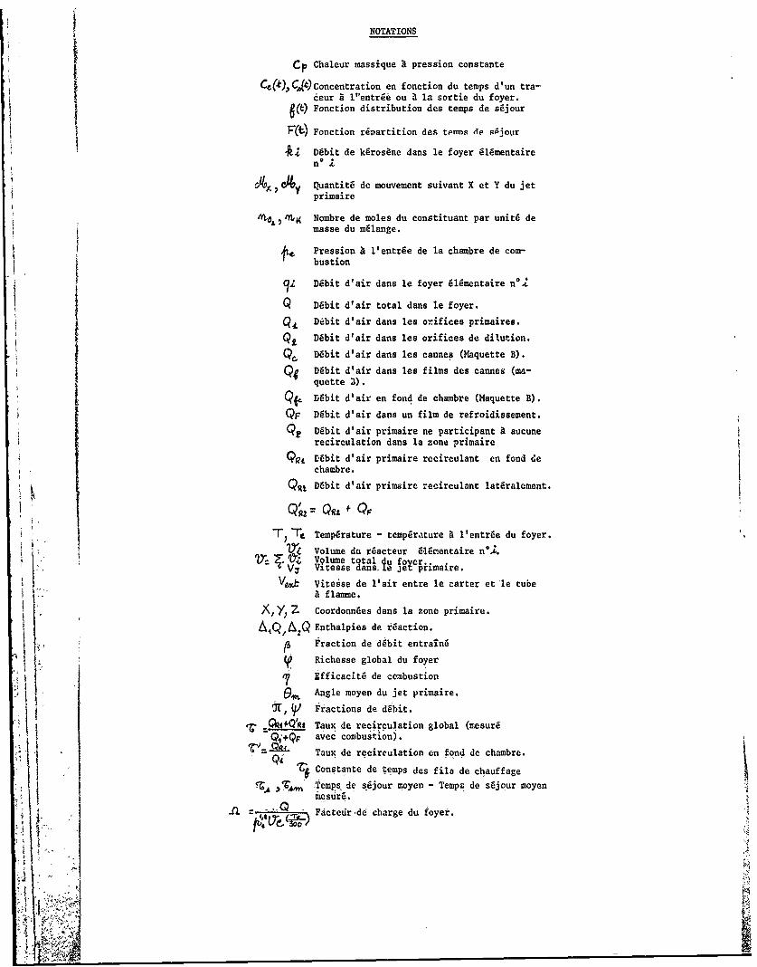
NOTATIONS

Cp Chaleur massique A pression constante

CO~),4(tPoncentration en fonction du temps d'un tra-ceur A l'entr~i ou A la sortie du foyer.

6 (k) Fonction distribution des temps de s~j our

r~)Fonction riDartition des tenins die Ojour

M. dit de kfirosbne dans le foyer 6l6mentairen*

t Ay Quantit6 de mouvement suivant X et Y du jetprimaire

ft,7~g Nombre de moles du constituant par unit6 demasse du milange.

S Pression A l'entrfie de la chambre de cown-bustion

3 DZbit dtair dans le foyer 6ldmentaire n*2

Q Deit d'air total dans le foyer.

Debit d'air dans les orifices primaires.

Q't bit d'air dans lea orifices de dilution.

Deb it d'air dana les cannes (Maquette B).

Q; bit d'air dans lea films des cannes (ma-quette 3).

Dfibit d'air en fond de chambre (Maquette B).

QF Deit dtair dans un film de refroidissement.

Lo DMit d'air prizuaire ne participant A aucunerecirculation dans la zone primaire

Qsu Meit d'air primaire recirculant en fond dechambre.

QMDeit d'air prilnaire recirculant latdralement.

T, T. Temprature - tenip~riture A l'entr~e du foyer.

Z Volume duracteur 616entaire n*LVU.Vitssedana.l Jey primaire.

Veotb Viteise de l'air entre le carter et 'le tubeA flaimme.

A, YZ Coordonn~es dans la zone primaire.

4Q ~ Enthalpies de teaction.

Fraction de debit entraTn6

Richesse global du foyer

ifficacitd de combustion

SAngle moyen du jet primaire.

t 9 ractions de de?,it.

'C -a1+4R2 Taux de recirculation global (mesurgi 9,,+QF avec combustiion).

Taux de recirculation en fond do chambre.

Constante de temps des fils de chauffageTA, -temps do sdjour moyen Tempa de s~jqur moyen

41acteiir~dd charge du foyer.

I - INTRODUCTIONKLa privision des performances des foyers de turbomachine tant dui point de vue de l'effi-cacitg de combustion que de la pollution exige jI,2]exige une technique de mod~lisation guffisamment pritci-

se et rdaliste pour tenir compte des divers ph~nomanes dans chaque partie du foyer.Parmi les mithodes demod~IisationE 3 1., on peut distinguer deux groupes prinaiipaux

le premier consiste A repr~senter chacune des regions principales du foyer par une suc-

du foyer ou meme effectuer une optimisation de ses performances [4]

-selon le second groupe de m~thodes, on 6tudie dans le d~tail chaque region principaledu foyer ainsi la zone primaire ntest plus consid~r~e comme un ou plusieurs r~acteurs 6l~mentai-res mais comne une zone de combustion turbulente dans un 6coulement tridimensionnel (7-8-9-10-11].

La validation de ces modales n~cessite l'exp~rimentation de diverses chambres de combus-tion. En particulier, is mise en oeuvre de mod~les nonodimensionnels (succession de r~acteurs 6id-

mentaires) denande une bonne connaissance de la dynamique des gaz dans le foyer. Ainsi ii eat ndces-Isaire d'avoir de3 informations concernant lea riacteurs Slimentaires :emplacement, volume, tempsde adjour, etc...

Dans ce but, une adrie de maquettes(figure 1) a 6tg essayge. La zone prinaire d'un foyerde turbomachine A a 6t6 matgrialisge sous forme de montages pouvant rdpondre A diffdrentes utili-sations

-maquettes ou demi-maquettes fonctionnant en air froid pour des nesures de vitesse, deturbulence, de temps de adjour par thermodilution.

surr la -demi-maquettes placges en tunnel hydraulique afin de visualiser l'dcoulement et d'y me-srrlatemps de sdjour par comptage de particulei et traitement du signal viddo.

ne anly~mquete compl~te 6tudide avec combustion (relev6 des performances en fonction du rdgi-me anlys deIscombustion par sondages A l'intdrieur du foyer).

Ces diverses cxpfiriences ayant dnnd des rdsultats juggs trop lids A un type particulierde chambre, ceux-ci dnL. dtd poursuivia dana un foyer B (figure 1), cette chambre B eat ddrivde de Amais en diffare par

- le fond de chambre qui eat raccourei,- is prfisence de canne. a prdvaporisation qui remplacent lea Injecteura de carburant si-Ituds dana lea orifices primaireade A.-Lea orifices primaires qui sont riduits de maniare a conserver le ddbit primaire malgrg

l'introduction d'air par lea cannes a prdvaporisation,Le but de cette 6tude ne consiste pas A optimiser ni une chambre de combustion particuliare

iii un rnodale de calcul. Au contraire, on utilise un moddle volontairement simple dont la dfifinitiona appuie sur lea caractdristiquea agrodynamiques effectives des 6coulementa 6tudids.

A partir des rdsultats expdrimentaux recueillis dana lea chambres A et B, une moddlisationmonodimensionnelle a Wt glaborde pour chacune d'elles. Les diffdrences entre ces deux chambres et

leurs performances sofit diacutfies ainsi que lea rdaultats de !a moddlisation.

2.- ETUDE EX.PER1MENTALE SAN4S COMBUSTION2.1- Maoynsd'essai

Bien que ne permettant pas de prdsenter l'enaemble des phdnomdnes intervenant dana leadcoulements avec changement de densit6 et cindt ique chimiqw, Ies 6tudea par simulation sur modalesfonctionnant A froid constituent un o'jtil prdcieux pour la comprdhension de~ l'afirodynamique inter-ne des chambres de combustion. Pluaieurs 6tudes ont ddjA confira-d la similitude entre 6coulementsavec et sans combustion A condition que lea nombres de Reynolds foipida sur les conditions d'entrgesoient comparables [12-13-14]. Plusieurs maquettes semblables A celles fttdides en combustion ontdonc fait l'objet dt'essais aur lea deux installations suivantes

- un tunnel lydrodynamique- une veine adrodynamique

2. 1 .1- Tunnelhdo~anje

Sur un tunnel 1hydrodynamique semblable A celui utilis6 par H. WERLE 115] , nous avonsmi.. en oeuvre des techniques ciassiques de visualisation (filets colords, bullea d'air ou d'hydro-gdne par 6lectrolyse),pou'r prdciaer ia configuration de 1l*'6coulement. Lea visualisations qualita-tives sont compldtdessous un aspect quantitatif spdcialement utiliad pour lea mesures de temps deadjour par comptage de microparticules neutres via A via de l'dcoulement (16-18] . Lea tchniquesmises en oeuvre qui font appel au traitement de signaux viddo rdsultant des enregistirements des di-vers essais, sont largement discutds dana lea rdfdrences [1L et 20]

2.1.2- Veine a~rodnan12ue

La veine akrodynamique sur laquellepeuvent Btre montdes plusieurs types de-maqu tes[19] permet d'effectuer descartographies tr:,dimensionnelles de vitesse A partir d'un fil chaudtournant aelon une technique mise au nc'int au CERT [17] . Lea cartographies de vitesse sont compl6-tfies par des mesures de fonction de rdparcition de temps de sdjour obtenues par une technique on-ginale de traceur thermique par thermodilution (19] . Cette technique dont le principe eat reprdsent6a la figure 2 associe un chauffage de l'dcoulement par impulsions 6lectniques calibrdes sur des filsthermorgsistifs, une mesure de fluctuations de tempfirature par fi chaud a faible taux de surchauffeet uri 66hantillonnage par m~yenne fiumerique.

2.2- Rdsultants qualitatifs sur les visualisations

Compte tenu de la complexitfi et du caractare fortement tridimenisionnel de l'Ecoulement dans4 la zone primaire, les vicualisations sont indispensables pour permettre d'interprdrer lea diverses mesures(vitesse, temps de sdjour, etc ... ) effectuges en parallale. Elles permettent aussi de voir rapidementl'effet dti 5 une modification (gdom~trique ou cinfitique) sur l'ensemble de l'6coulement.

dtdeLa configuration de base A' est la configuration sans canne et avec fond de chambre allong6on 6tdeensuite 1'influence due A une modification de ces derniers points.

De nombreuses visualhsations par filets colores ont conduit A la description suivante del'6coulement. Cette reprdsentation qui montre le caractare fortement tridimensionnel de l'gcoulementcontraste singuliarement avec les schimatisationa habituelles (jet et tourbillon importants en fond dechambre). Lei jets primaires pdnatrent dans ia chambre en crgant un double systane de tourbillons

- 1atdralement , une paire de tourbillons d'axe OX, qui sont le siage de vitesses glevges,s'6tendent jusqu'A ia dilution et remontent en partile au fond de chambre (figures3 et 4). Le caractarefortement instable de leu'i surface de contact se traduit par une alimentation alternative entre cesderniers.

-par un idger m~uvement hdlicaldal en anoint, ces tourbillons font recirculer, en fond dechambre, une partie QR± du dfbit primaire Q, - Ce dfibit Q se retrouve en partie dans un tourbillonde petite taille d'axe OZ assurant ia continuit6 avec le prdcd~dent(tourbillon enfer a cheval).

L Ie reste du ddbit Q alimente une partie du fond de chambre de fagon instationnaire auvoisinage du plan de symdtrie entre orifices (.3)

-Dans leur parcie latdrale et aval, les tourbillons d'axeOX sont aiimentds par la fractiondu dabit primaire et travers~s en leur coeur par le debit Q.RI venant du fond de chainbre.

Enfin une partie Q. du d~bit primaire va directement vera Is dilution quaaiisent sans m~lange*avec le reate de 1'culmn primaire.

Ces divers commentaires doivent 9tre compldtds par lea deux remarques suivantes

11I est Evident que le passage entre Qj , Q', Qp eat plus continu qu'il n'apparat danala description prdcddente mais cetzte derniare a dfija 6tS effectuge dans l'optique d'une moddlisationpar combinaison de r~acteurs 6ldmentaires aliment~s de fagon discrate par diffdrenta d~bits.

-Une part importance du fond de chambre (figure 3) ne participe pratiquement pas A 1'6cou--lement et peut Btre considdrde comme une zone quasi-morte. Ceci nous a conduit A r~duire le volume dece dernier dana la'seconde maquette B.

En dehors de celle portant sur le volume du fond de chambre, la seconde modification..envisaggeconcerne is simulation des cannes a prdvaporisation. De nombreux essais ont Etd effectuds A divers d6-bits en modifiant lea deux paramatres suivants

ddbit descannes - Qc/Q3 (de 0 A 40%)position des cannes par rapport aux orifices primaires.

Un des r~lea des cannes 6tant d'am~liorer la recirculation du fond de chambre , on a donceffectud une Etude systdmatique permettant de positionner ces derniares de fagon A obtenir dans tousles cas de fonctionnement un d~bit QC alimentant le fond de chambre . Lea r~sultats de ces essais (18]ont conduit A faira d~boucher ces derni~res au 1/3 amont des orifices primaires.

Qualitativement, on ne remarque pas de diffirence notatle avec lea cas sans canine si ce n'estsur le fond de chambre, point sur lequel rous reviendrona par Is suite (temps de s~jour).

2.3- Masures de vitesse et rBpartition des dfibits

2.3.1- Hesures de vitesse

A Ia figure 5 sont prfisentds quelques rdsultats significatifs sur lea meaures de direction devitesse dana la zone primaire obtenues dans le cas suivant

configuration AV debit total 0,25 kg/s.* On y retrouve plusieurs 6idmsents obtenus par viaualis'ition (par exemple :tourbillons latd-

raux importants avec mouvemeut h~liqoIdal).iiUn parambtre important pour Is moddlisatio 'n,6tant la part de ddbit (Q 1%) recirculant en fondde chambre mais in ressortant ensuite (par opposition au ddbit entratin qui reste dans la zone de re-circulation), noui avons cherchS 1 le meaurer

2.3.2- Mesure degq.

Deux mfthodea compldmentaires ont Wterploydes pour cette mesure

a) a partir des sondages de vitebse (19]

I ~ La premiare mdthode consiste A determiner A partir des cartographies. de vitease et de s"1trace" dana le plan Y -0, is surface de asparation entre les deux fractions de ddbits suivantes

Iiet ev4 G~'Q

h Les rdsultats de ces mesures, correspondant A ia maquette A, sont prdsentds A la figure 6 enfl fonction des param~tres gdomdtriques (h/H ou n t.idacqe V)

~ ;..b) a partir des temps de s~jour

Dana le, cas ott, comme pour is maquette B', le volume occupl en fond de chambre par l'dcou-lementlement eat connu, la mesure de (temps de sdjour moyen en fond de chambre.) pernet d'accdder 5 Q.

+______

On mesure de fagon semblable Q parQ1 fQRj Q

Les essais obtenus sur un bane hydraulique (§242) sont pr~sent~s A la figure 7 pour 0. Q-//,35 2.d'n Les valeurs pour Q,.= 0 sont compatibles avec les essais pr~cedents, ce qui confirme l'existence

d'nvolume mort en fond de chambre dans le cas de la maquette At. On notera avec intgr~t lea ivolutions

de Q~tI Q, Q avec Qc/Q-.

2..4- Yeue-etmsde sgiour

Pour completer les essais en vue de parfaire la mod~lisation, nous avons cherch6 a dater- "miner la fonction de distribution de temps de s~jour ; (t) (ou F (a)fonction de repartition) en di-vers point du foyer. La technique, classique dana son principe, consiste a injecter en entree une fai-ble concentration Ce(-C) d'un traceur que V'on d~tecte en sortie (CA(t)); on montre ais~ment que dansce ca [ 21]

C4 60Sur ce principe et compte tenu des imp~ratifs ligs A ces essais (emplacement, temps de rdponse ...)

nous avons mis en oeuvre deux techniques originales de mesure.2.4.1- mcs res su banc agrodynam*se.

La techniqte par thermodilution dana laquelie C:,L)correspond A un 6chelon descendant per-met done d'obtenir rapidement, en un point quelconque du foyer, la fonction de repartition de temps deatjjour F (.t) entre l'entr~e de la zone primaire et le point de mesure par

F -t CA'(4)

cas ', - 25 rn/a. Cette valeur correapond A un optimum compte tenu du niveau du signal de temparature

A mesurer et du rapport entre le temps de s~jour moyen et la constante du temps des fils de chauffagede 1'gcoulement.

2.4.1.1 - Mesures en aval de la- zne primaire

Pour tous lea points aitu6s en aval et dana la zone de dilution, lea courbes de d6-croissance en temp~rature sont semblables et prfisenten t lea caract~ristiques suivantes (fig. 8).

I/ aux premiers instants suivant le refroidiasement, la tempdrature conserve la valeurinitiale Te pendant une dur~e Ato d~pendant du point de mesure,

2/ vient ensuite une zone de transition de 10 A 20 ma,

3/ enfin, suit une zone de dficroissance plus ou momns exponentielle dont la conatante

de temps mesur~e , pratiquement ind~pendant6 du point de mesure, vaI ut sensiblement

155 ma (valeur exacte :115 d 120 ms) (y compris la zone de transition).f

Lea courbes de d~croissance en .tempgrature comportent deux types d'informationaconcernant d'une part, la fonction de r~partition de temps de s~jour en sortie dezone primaire et d'autre part, la nature de la zone de dilution.I

En effet, la fraction du signal correspondant aux portions (2) et (3) ainsi qu'a4 une partie de la zone (1), eat caractfiristique de la fonction de distribution de

temps de s~jour en sortie de.12ne piie.Ce signal, 'arrivjant A l'entr~e de la zonede dilution eat ensuite translt dan ctte derniare, sins deformation et sur unedur~e d~pendante de la distance du point de mesure a l'entr~e.Ce r&cultat eat confirmfi par le trac6 (fig. 8) do At o en fonction de l'abacisse. Aprbsune zone de transition localis~e au niveau des orifices de dilution, ces c6urbes qua-siment lin~aires dana la zone de dilution ont une pente dont la valeur

- "' 3,4, m/s

semble tout a fait compatible avec la vitease moyenne de l'dcoulement (3,1 m/s) danacette zone et conduisenit A modfiliser la dilution comme un rdacteur de type piston.

2.4.1.2 - Mesures en sortie et dana la zone Primaire

Led courbes de d~croiiaance en temfiprature (fig. 9) sont semblableas aux pr~c~dentesminis 1ci 'C et Atiddpendefit du point de mesure. En sortie de zone primaire, lea 6carts entre courbeaymontrent bien le civactare inhomogane de 1'6coulimn

- Rsultats ideatiques dans lea tourbillons iatfiraux (.i' 10 a i5)-Dans le plan de sym~trieZ - 0 des relevfis diffirents correspondant a des trajeta d' cou-

lement difffirents (la fraction de Op inteicepdeq se ti~aidisant-par une diiainu.tion de Tp au!"-ente vera la.7one-d'imoact des jets 7 -0').

On retrouve cette disparitE dana la zone primaire-temps de se~joui moyen tr6s variable* (200 ma en fond de chambre, 140 ma a 170 ma

lat~ralement, 100 ma a 140 ma en aval des jets '(fig. 9) )

-courbes iso Ato (fig.1O) permettant de retrouver la prdaence de tourbillons latii-raux (coupe B -B') et la convergence di 1'6coulement entre orifices en fond de chambre~coupe A-A,').

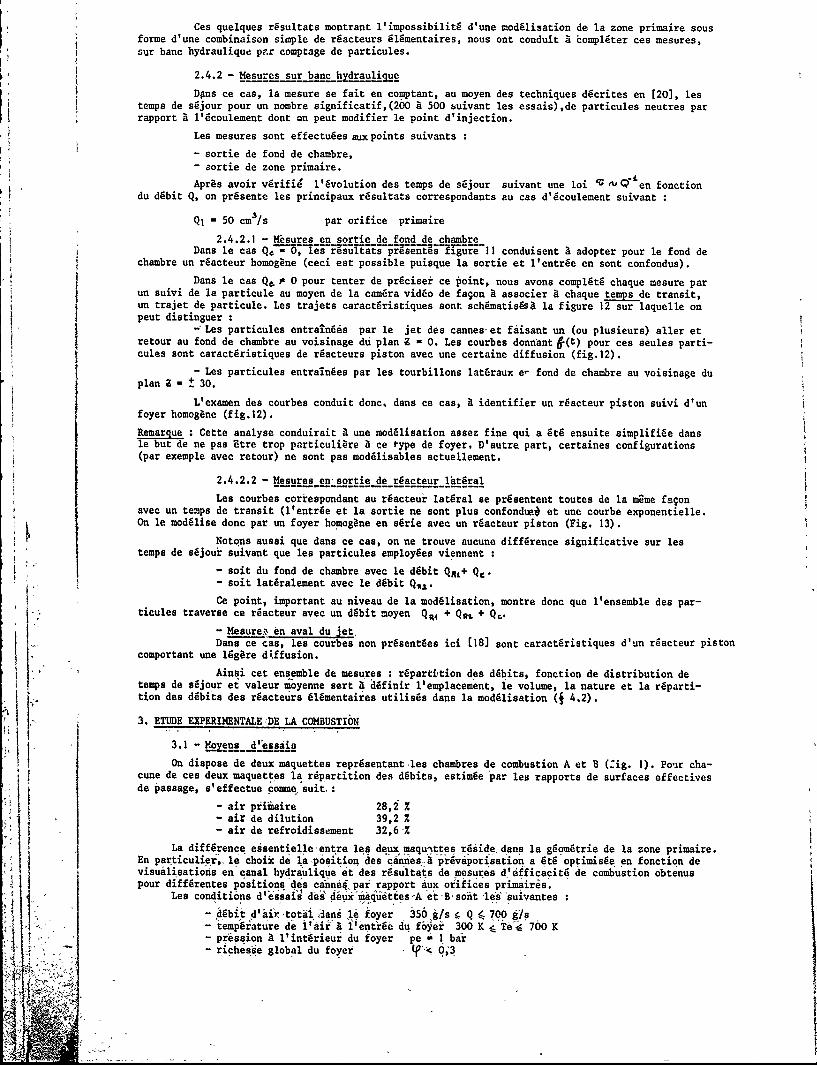
Ces quelques r~sultats montrant 1'impossibilitE d'une mod~lisation de la zone primaire sousforme d'une combinaison simple de rdacteurs filimentaires, nous ont conduit 1 compldter ces mesures,stir banc hydraulique pzr comptage de particules.

2.4.2 - Mesures stir bane hydraulique

Dpns ce cas, la mesure se fait en comptant, au moyen des techniques ddcrites en (20], lestampa de sdjour pour un nombre significatif,(200 A 500 buivant las essais),de particules nautres parrapport A l'6coulement dont on petit modifier le point d'injection.

Lea mesuras sont ef fectu~es aux points suivants

- sortie de fond de chambra,- sortie de zone primaire.

Apras avoir vdrifie' l'ivolution des temps de s~jour suivant tine loi ' tq4'en fonctiondu ddbit Q, on prdsente les principaux rdsultats correspondents au cas d'6coulement suivant

Q= 50 cmh/ par orifice primaire

2.4.2.1 - Meaures en sortie de fond de chambraDana le cas Qj= isreuttsp0en7 ir conduisent a adopter pour le fond de

chambra tin r~acteur homogine (ceci eat possible puisque la sortie et l'antrge en sont confondus).

Dana le cas Q0, 0 pour tenter de prdciaar ce point, nous avons compldtfi chaque mesure partin suivi de la particule ati moyen de la cam~ra video de fagon A associer a chaqtie temps de transit,tin trajet de particule. Les trajeta caractfiristiqies sont schimatis~sik la figure 12 stir laquelle onpeut diatinguer:

-Les particules entralln~is par le jet des cannes-at faisant tin (oti plusiatirs) aller etretour aui fond de chambre ati voisinage du plan 9 - 0. Lea courbes donnant Pf-t) pour ces aetiles parti-cules sont caractdriatiquea de rdacteurs piston avec tine certaine diffusion (fig.12).

-Les particulas entralinfes par lea tourbillona lat~raux e- fond de chambre aui voisinage duplan a - + 30.

L'exanien des courbea conduit donc. dana ce cas, a identifier tin r~acteur piston suivi d'unfoyer homogane (fig.12).

Remargue :Cette analyse conduirait A une moddlisation asaz fine qui a 6t6 enauite simplififie danale but de ne pas Btre trop particulikre a ce type de foyer, D'autre part, certainea configurations(par axemple avec retaur) ne sont pas modilisables actuallemant.

2.4.2.2 - Mesures en-sortie de rfcteir lAtfiral

Lea courbea cariespondant ati r~acteir latdral se prdsentent toutas de la mime fagonavec un temps de transit (l'entrfie at la sortie ne sont plus confondw.j et tine courbe exponentielle.On le moddlise donc par tin foyer hornogane en sfirie avac tin rdacteur piston (Fig. 13).

Notons aussi qua dana ce cas, on ne trouve aucuna diff~rence significative sur leatemps de s~joui suivant qua lea particulas employ~es viennent

- soit du fond de chambre avec le ddbit Q~j+ Qc.- soit latfiralement avec le debit Q1A.Ce point, important aui niveai de la modelisation, montre done qua l'ansemble des par-

K-ticulas traverse ce rdactaur avac tin debit noyan QM;t + Qt. Qc.-Masure,, 6n aval duet

Dana ce cas, lea courbas non pr~sentges ici (18] saint caractdristiquas d'un rdactaur pistoncomportant tine l~gare dtkffusion.

Ainsi cat ensemble de mesures :r~partition des debits, fonction de distribution detamps de afijour at valaur manne saint a ddfinir l'emplacement, le volume, la nature at la rdparti-

Iftion des debits de s rhacttirs 616mentaires titilisga dana la mod~ljaation (J 4.2).

3.* ETUDE EXPERIMENTALE DE LA COMBUSTION

3.1 - Moes_ d 'esss

On dispose de deux maquettes reprgsentant las chambres de combustion A et B C--ig. 1). Po'Ir cha-cuna de ces datix maquattes la rdpartition des d~bits, estimfe par les rapports de surfaces effectivesde passage, a'effectue coma, suit,-

- air pfiaire 28,2 Z- air de dilution 39,2 %- air de refroidiasemant 32,612

La difference essentiallee4ntre lea deux maqu'.ttes rid ans la gdomatrie de la zone primaire.

En particulier,. le -choix de la position 'des 'c~nsApriviporisation a 6t optimisge a e nct devisualisations en canal bydriulique at 'de's r6dsult'ats de mesures dfficacit6 de combustion obtenus

prisio A 'in~riurdu foyer pa i1 bar

Les conditions d'essai sont contr~ldes en temps reel pendant les essais. Pour divers r6-gimes du foyer, et en diverses positionsde sondage A l'int~rieur de la chambre (fig.1), on prdlave

j.lea produits de combustion dana une petite bouteille. Ces fichantillons sent analysis par chromatogra-phie en phase gazeuse. Un premier chromatographe permet de doser le gaz carbonique et le m thane.Un second chromatographe s~pare oxyde de carbone, azote et oxygane tandis qu'un tioisi~me isole l'hy-drog~ne. L'analyse des oxydes d'azote est r~alisge au moyen d'un appareil classique 9 chimilumines-cence.

Deux types d'exp~riencesont fit6 conduites dans ces chambres de combustion. Des exp~riencesd~crivent l'~tat du foyer du poit.t de vue des espaces chimiques pour -un regime de fonctionnement par-ticulier. Cette s~rie d'expgriences a 6t r~alis~odans la maquette A et reprise d'une mani~re plusd~taill~e dans la maquette B. La seconde sdrie d'experiences avait pour but d'6valuer le fonctionne-ment global de la chambrL de combustion A. Pour diffdrents regimes - c'est-a-dire diff~rents pointsde fonctionnement caract~risgs par Q, Te et Y- on relave des efficacit~s de combustion, niveaux depollution en des positions caract~ristiques 1 l'intgrieur du foyer(entrge et sortie de la zone pri-maire, sortie du foyer).

3. -Anls el cmuto ' int&rieur de la chambre

Lea points de sondage a l'intdrieur du foyer (fig.1) sur toute l'envergure dc celui-ci sontchoisis en fonction des r~sultats desvsualisations. Ainsi les positions 1, 2, 3 correspondent au fondde la chasibre, lea points 4,5 et 6 A l'aval des orifices primaires et la position 7 A la sortie du

0foyer.Le rdgime pour lequel les sondages ont 6t effectufis correspond a l'adaptation de la cham-

bre de combustion A (Q - 530 g/s ; To - 545 K ; j=0,226). En vue de comparer lea r~sultats danalea chambres A et B, ce regime a 6t6 conservd pour lPs essais dana la maquetto B.

Lea sondages effectugs en fond de chambre position 2ne permettent pas do d~celer une orga-nisation tras nette de 1'6coulement. L'alimentation alternge des tourbillons occupant cette regionpar le debit Qt, peut expliquer cette absence d'organisation. La richesso y eat toujours plus grandeque I et le degr6 d'avancement de la combustion inf~rieur A 0,5.

En aval de la zone primaire, le plan de sym~trie du foyer (Y -0 ; position 5) et le plancontenant lea axes des tourbillons lat~raux (Y - ± I5 ; position 4 et 6) sent explores. Apras avoirv~rif i6 la syn~trie du f oyer pour lea positions4 et 6, on pout voir pur la f igure 14 quo 1'6coulement ea tmaintenant bien organia6 autour des jets d'air primairo. En effet, la p~riodicit6 do la richesse eat

k la mame que celle de l'injection du carburant qui se aitue au niveau des orifices primaires des chain-bros A et B. Le choix du point de fonctionnement du foyer ((? 0,22) conme 6tant le point d'adapta-tion de la chambre A eat justifi6 par le fait que V'on retrouve bien une richoase inoyenne proche deIA la sortie de la zone primaire. On retrouve 6galement quo le ddbit Qc a modifi6 l'adaptation de lachambre B puisque la richesse nayenne nWest plus quo 0,61. En re alculant le raep4Zrts des debits d'air6valu~s a ce niveau pour lea configurations A et B, on obtient I, 48 qui eatde l'ordre du rapport *1,64 (QF eat le debit dana un film do refloi issement ne 1, chambre,Q. dana celui de la cixnne et Q gole ddbit dana le fond de la chambro B -voir mod~lisation -(# 4.2)

Lea relevds effectu~s en position 5 (fig. 15) donnent des r~sultats tr~s diffdrents de ceuxde la position 4. Cotte partie du foyer eat ,en effet, directoment alimentge par in fraction desjetsa primaires non carbur~e et nerecirculaitpas (QL,). La richesse moyenne nWest plus que de l'ordrede 0,1 pour lea deux chambres A et B. De plus la richesse 6tant minimale dans l'axe des jets priinsi-

tea, on peut dire quo le carbuiant pr~sont A cet endroit eat amen6 par diffusion issue de tourbillonslatdraux et non par convection A partir des orifices prinaireG.

3.3 - Influence du r~gimE sur le fonctionnement de la-chambre-- - - - - -- - - - -

foyer Cos oxpfiriences avaient pour but de determiner l'effet du r~gime sur lea performances dufyr(rendement, pollution). Ainsi pour chaque point de fonctionnement du foyer, on relive lea va-

leurs moyennoa des concentrations sur une traversde aux points 2, 4 et 7 do la maquette A, cc qui Per~met d'atteindre le degri d'avancement de la combustion. Des relevfis du mime genre ont dgalement 60effectugs~sur la maquette B mais d~n mani~re momns syst~matique. La figure 16 montre l'effet do larichosse sur l'nficct de combustion. Ces r~sultats exp~rimentaux qui pr~sentent une dispersionimportante en raison dos h~t.6rog~n6!tds .1 lintfirieur du foyer sent compargs aux predictions d'un cal-cul (voir 4.3).I: 'gvolution des oxydes d'azote en fonction do la richease (fig. 17) s'intorpr~te assez fa-cilement. L'accroissemont du NO avoc la richessoe dure jusqu'5 une richosse voisine de cello do l'adap-tation (T - 0,22). Au-dels do cette valour NO dttcrott tandis quo NOe..continue do croltre. Cot acerois-senent s'expliqu6 par l'apport d'air d6 dilution a l'aval do la zone primaire :le NO contizizedo a'oxy-der en NO2..

4. NODELE MONODIMHENSIONNaLDE.-FOYER

4.1 rPrincie de la modglisation

Lea r~sultats prdsent~s .et discut~s dana los paragraphes pr~c~dents ont permis des recou-pements qualitatif a avec lea essais en a~rodynamique pure. Dana le but d'avoir uno interprdtationquantitative. du comporteme *nt du foyer, ufie mod~lisation simple a 6t6 entreprise. Ce typo do mod~lisa-tion qui consisti Arepefsenter l0 foyer par une sfirie do foyers 616mentaires s'appuie sur l'ensembledes renaeigncments acq'ui's au cours des visualisations, meaures a~rodynamiques, etc...* En of fet, la

dsrt'isai d- la chanr do 'Combustion en r~acteurs 616mentaires eat facilit~e par los visuali-sations en tinne1 hydraulique qui ont localis6 l6a zones oe recirculation. Les mesures do temps dor~ijour out permis de d~terminer la nature des r~acteurs 6i~mentaires-(homog~ne oude typo piston).De ma me'le choix, dilarpaitibn de's debits datis ces r~acteurs oat la consequence des mesures dotaux do recirculation .

W-

Cette moddlisation semi-empirique s'appuie sur les travaux de R. BORGHI [411. Rappelons-enbri~vement le principe g~n~ral :on reprdsente la chambre de combustion par une suite de ftr~aceurschimiques de volumes variables. On peut introduire dans chacun de ces foyers des entrdes d'air ou decarburant qui simulent dilution, cannes A prdvaporisation... .On peut calculer les conditions d'en-trde du ikme r~acteur A l'aide des conditions de sortie du rdacteur Ci - 1) et des conditions de l'a-limentation en air, qZ et~ea carburant tZ de ce ii~1e rdacteur. Il suff it d'6crire lea bilans 6ner-gdtiques et de masse. Le ie~ne rdacteur est cazactgris6 par q., k., Tez tempdrature d'entrde, et l7llevolume du r~acteur. Le problame consiste A d~terminer le degre- dfavancement de la'combustion Slzat-teint dans chacun des rdacteurs pour un temps de sdjour donnfi

(avec

Les ph~nomanes de combustion et de pollution dana le foyer sont scbdmatisgs par deux rdactionschimiques

Ve,+ ?40.1 NO~

Les lois de proaiuction utilisges dons le calcul sont

-pour la rdaction gnergfitique (30]

et Wi. 7'Z M% ,)(T

L'accroissement de temperature provoqud par la combustion est 6gal a

ou/=ee + A 2Q ft,1.N 2 ,-iNJ e_

et 4,5 -4,5

-pour la r~action de pluin(tn~canisme de Zelov oc )W, 6 14 42 6- o

6 2 Q -A,S AO5

La mdthode de calcul de et des produits polluants eat indiqu~e par R. BORGHI dane 4 .

4.2 - A Dlication aux fovers 6tudi~s

L'ensemble des expdriences en air froid et en tunnel hydrodynamique conduit A un mod~ledifferent pour chaque chambre A ou B. Ces modales sont ddcrits figure 18 pour l'emplacement des r6-acteurs et figure 19 pour la rdpartition des ddbits.

La zone primaire de Ia maquette A eat diviade en trois rdacteurs 616mentaires. L~e ddbit d'airprimaire Q3. se partage conime suit

- QjR. qui alimente le rdacteur I (celui-ci recevant de plus le carburant)- Qjj. qui constitue une partie du debit total Q'.R.alimentant le rdacteur 3 Wi%% , QSL + Q,).

- Qp qui ne pa1rticipa pas a !a recirculation d~hs la zone primaire va directement dans ler~acteur 4,+ ~~Ce rdacteur 4 constitue le premier 6ldment de la zone de dilution. II regoit un dfibit

Qp+Q/+Qj (Q2. ddbit total de l'air de dilution). Le r ,acteur 5, deu-xi~me fil~ment de la zone dedilution regoit Qi /2 -& QF tandis que le rdacteur piston 6 n(esi plus alimefit6 que par le dernierfilm de refroidissement. Les r~sultats des miesures de temps de s~jour (fig.8) justifient l'assimila-tion du r~acteur 6 A un rdacteur piston. V QR4

Le choix de QR, ayant 6t6ddtermin6 par lea mesures de '- , ~ reitait a ddfinir. Untaux de recirculation glba" = d2~ td dvalu6 indirectement lors des essais avec combustion.

Cette mdthode bas~e sur la propriftdde l'eau do r~duire lea oxydes d'azote dams une chaambre de com-J t I bustion eat expos~e dana [ 3911. La valeur de $ retehue pour la modglisation eat 0,7 tandis que '=0.,36.

Cette valeur'T= 0,7 eat compatible avec cello de &L.. atirnde pour Q,./Qj -0 (fig.?). Lea vo-

lumes Lan dgutsd do ~aiohd chab±b et des temps de sdjour mesurels.1amdl-aind6l aui B .est pI lui comple'xe. La prieici des, caiines modif ie non seu-

lement lea dabits QRI, Qk, elt Qp maii aw~si la disporition et.la nafte des r~acteurs dana la zoneprimaire. Le I agcteifr piston,. I et le rhateur h,)mon 2 iiulent 1e food de 1a chambre. Le rdacteurI ettravers6 pai, Q, ~dit caiihe, augmnne r~ action -7 d&e6i'_ t_ eiaf' Q,' ~ q '1/3) et du' carburant. Leracteur 'iqit Qj + Qj'. ei la fraccion' (3 -1ir ') d6 Q~. Le ddbit'alimrnint,3,est constitu di

Rt Q R+ Ce rdacteur eo-t sii u rdacteur pitn 4.Lsralur uints sock 'ide tiques

Cependant, cette modfilisation retenue pour t u de la combustion prdaente des diffdrencespar rapport A la moddlisation originelle sans combustion, en plus de. la .pr~sence des ddbits Q.j Qfcetd apras lea mesuros de tempa de s~jour). D6 plus, dams la moddlisation ave combustion, on a simpli-

fi6 la rdpartition des ddbits en fixant W1= 1. En fait, paur prendre en compte la valeur rdellsejY= 0,6,ii suff it de choisir les volumes des r~acteurs I et 2 en zccord avec les temps de s~joui mesurgs ef-fectivement pour q=0,6.

Il est possible dt retrouver la fonction de transfert qui calcule la distribution des tempsde s~jour en a~rodynamique pure dans ls foyer A A l'aids d'une modfilisation diff~rent idgarement decelle avec combustion (fig. 19);

- un r~acteur fictif simule is constants de temps des fils de chauffags utiiisds pour lamesure des temps de sijour (S 2.4'.1).

- le rdactsur I - 2 rempiace les rdacteurs I et 2 du cas avec combustion.

- ie rdacteur 3 est suivi maintenant d'un, rdacteur piston 3'

- is rdacteur piston 4' regoit le ddbit Qp qui, dans is cas avec combustion, alimentaitsans intermddiaire la zone de dilution.

Les rdsultats du caicul sont compards aux expdriences effectuies a la sortie de ia zoneprimaire (fig. 20) :l'accord satisfaisant dimontre que iedi~coupagede la zone primaire en foyers 61d-mentaires peut reprdsenter la chaxabre de combustion A.

4.3 R16sultats des calculs

L'dtude de la stabiiit6 du foyer a 6t6 entreprise avec ies mod~les de chambre A et B etles r~suitats num~riques et expfirimentaux sont compargs sur is figure 21. L'accord pour le foyer Aest bon mais un peu moins satisfaisant pour B quoique !s tendance soit correctement pr~dite (richesseflimite d'extinction pauvre pratiquement constante avec is regime). Ceci constitus une nouvelie justi-fication a postgriori des moddlisations retenues. En offet, ce sont les r~acteurs num6:otAds I dans ismoddiisation de is figure 19 (rdacteur h'omogane pour A et piston pour B) qui conditionnent ces iimi-tes d'extinction. De pius, i'utilisation des valeurs Q~t et Qc +1 Qll trouv~es lora des essais afroid, comme debits alimentant ies rdacteurs 1 de A et B n'est p5 itrrdhliste.

La p-6diction des performances globales du foyer est donng figure 16 pour ce qui concerns1lniluence de YQ sur i'efficacitfi de combustion 4 i'entrde, sortie ds is zone primaire et sortie dufoyer. Dins ces deux cas de chambre de combustion, on constate un bon accord pour i'sntrge ds is zoneprimaire. Les rdsultats sont momns satisfaisants en sortie de is zone primaire. La moddlisation de iachambre B qui eat pourtant pius fine que cells uciiisds pour A (pas de r~acteur piston en sortie dur~acteur 3) ne donne pas des rdsuitats meilleurs. La raison ds cette dispersion doit Btre cherch~e au

Lnivsau des hypothases introduites pour lea reactions chimiques. Ces hypoth~ses sont insuffisantespour prddire misux que des tendances. Ceci eat encore plus net pour la prddiction des oxydes d'azote(fig. 17) pa is m~canisme de Zeidovitch ne peut prendre en compte is formation des oxydes d'azote Afaible richesse. MalgrC ce d~faut, qui pourra Ztre filimind par introduction d'uns cin~tique chimiqueplus compl~te et r~aliste, is tecnnique de moddlisation adoptds permet de reproduire fid~ie'sent lsatendances de comportement de chambre de combustion de types diff~rents. Ainsi l'am~lioration de per-formances en passant de A A B eat bien rendue par cette modglisation au prix d'un calcul simple etd'bypothases limities 6tay6 e par des eipgriences.

5. CONCLUSION

Dans is but de vAider un mod~isparticuli~rment simple de chambre de combustion , deux en-sembles d'expdriences ont 6t6 conduits sur des maquettes sch~matiques fonctionnant avec ou sans com-bustion. iss principaux r~sultats sont les suivantsz

Les visualisations hydrodynamiques compldtdes ensuite par lea cartographis de vites~eont conduit a une description relativement fine de lls~rodynamique dans is zone primaire. En parti-culier, on a mis en evidence is double sysame tourbillonnaire alimentant is zone primaire d'une parten fond de chambre, d'autre part latdralement. La rdpartition du d~bit primaire dans les diffdrenteazones a Vu Btre 6valu~e ainsi que lVinfluence de divers paramatres (angle de jets, ddbit et positiondes caunes A1 prdvaporiaation).

Ces mesures ont dtd complitdes, toujours a froid, par deo mesures, en tout point de !a chain-bre, de fonction de r~partition des temps dle sejour obtenus par diverasa techniques.

La comparaison avec les essais en combustion a 6d effectude en estimant dana ce cas isddbi reirci~ ina qu denomreu prl~vmens (O, O1,CO, C02, N2, 02) en divers points choisis en

fonction de I'afirodynaaique. Pans cc dernier cas aussi, on a pu6aurl~ouindspromne

fyrLe madale monodimensionnel utilis6, qui diff~re par certains points des sch~mas habitusile-ment employds, a done dtC dlaborS A partir de ces diverges donne-es experimentales. Le modale permet

a aussi de calculer les performnances 'giobales du foyer ainsi que le's fonctions de distribution de tempsde sdjour en sortie de rdacteurs 616mintaires. Bien que is modale utilisi soit volontairement simpli-fiii, en particuiier pour l'agrodynamique (ii ne prend pas en compte tous lea rdsultats obtenus en par-ticulier is taux de debit entraTnd) et ia ch 'imie (oxydes de carb 'ons et NO prdcoce), les r~sultats ob-tenus sont en bon accord. Cependant, une tells mod~lisation 616st appiayge sur l'analyse de i'gcouie-ment faite au prdalable. Ii east probable'que pour 6tudier une autre chainbre, ii faudrait refaire cette6tude ; en particulier, Is prdsence d'injecteurs a6rodynamiques ("sivirlir") changerait is dynamiquedes gaz. Pour s'affranchir de cette analyse agrodynamique, ii faut faire des calculs tridimensionnels

beaucoup plus compliqu~a tels que deux actuellement ddveloppfis a 1'ONERA [It ].

REFERENCES

[1 ] A. QUILLEVERE- "Developpement des chambres decombutstion a haute intensit6" AGAPRD Conference Pro-ceedtags no 34- "Advanced Components for turbojetEngines" - Sept. b8 - Toulouse.

f2 ] A.M. MELLOR - "Gas Turbine Engine Pollution""Progress in Energy Combustion Science" - 1976Vol. I p. 11I-133 - Pergamon Press.Vol I j11 -

[3 ] J. ODGERS - "Combustion modeling within gas tur-bine engines" - AIAA - 15 th Aerospace SciencesMeeting, Los Angeles (24-26 january 197;).

[4 J R. BORGHI - "Etude thgorique de l'opLimisationde la combustion dans les foyers de tutbomachine"Acta Astronautica, vol. 1 (1974) p. 667-685.

[5] 1 W. S. Y. HUNG- "An experimentally verified NOxemiss:4on model for gcs turbine combustion" -

ASME Paper 75 - GT - 71

(6] J. SWITHENBANK, I. POLL, M.W. VINCENT,D.D. WRIGHT - "Combustion design Fundamentals"14th symposium (International) on combustion-p.627.

[7] A.S. NOVICK, G.A. MILES, D.G. LILEY -

"Numerical simulation of combustion flow fieldsa primitive variable design capability" - Journalof Energy - vol. 3 - no 2 - March-April 1979-p.95-IO5

[8] W.P. JONES, W.C. CLIFFORD,C.H. PRIDDIN,

R. de CHAIR- "A comparison between predicted andmeasured species concentrations and velocities inA research combustor" - Symposium AGARD sur leshautes temperatures dans les turbomachines -19 - 23 septembre 1977 Ankara

[9] M. A. SERAG ELDIN, D.B. SPALDING- "Predic-tion of the flow and combustor processes in a threedimensional combustor chamber" - Imperial collegeof science and technology HTS/76/3- F~vrier 76.

[10] A. ELLAIL, A.D. GOSMAN, F.C. LOCKWOOD,I.E.A. MEGAHED- "Description and validation ofa three dimensional procedure for combustion cham-ber flows" - Journal of Energy - Vol. 2 - n 2 -March-April 1978 - p. 71-80

[0] 1 F. HIRSINGER, H. TICHTINSKY - "od6lisationde zones de combustion en regime instai'nnaire"AGARD - 54th (B) Specialists' Meeting or. combustorModelling - Cologne 1979.

[12 ] A.J. GERRARD - "Utilisation des modales hydrau-

liques pour l'6tude de l'dcoulement des fluidesdans un grot'pe moteur at une chambre de combustion"N.T. Hispano-Suiza 21.6.66.

[13] E.F. WINTER et al - "Apparatus and techniquefor the application of a water flow system to thestudy of, aerodynamic system" - Bristish journalof applied physics. Juillet 1956.

[14 ] KENNEDY - "Ramburner flow visualizations studie5"I I th JANNAF Combustion Meeting - vol. 2 Pasadetiai Sept. 741.

[15 ] H. WERLE - '!Le tunnel hydrodynamique au service

de la recherche agrospatiale" - Publication ONERA

B no 156 (1974)

I b] A. GIOVANNINI, P. HEBRARD - "Etudes fondamen-tales d'&coulements dans les foyers de turbomachine"Rapport CERT no 3/2062 DERMES avril 1978.

v [17 ] P. DAUGA - "Angmo. trie a fil chaud. M1-thodes de mesure directionnelles" - Thase(Toulouse 1975).

[ 18] C. LE MENAHEZ, A. MIR- "Afrodynamiqued'une chambre de combustion" - Etude appro-fondie - ENICA Toulouse (1978).

[19] P. HEBRARD, P. MAGRE, G. COLLIN-"Analyse et modlisation de l'Ecoulementdans un foyer de turbomachine" -La Recher-che Arospatiale no 1978-5.

[20] A. GIOVANNINI, P. HEBRARD,G. TOULOUSE"Quantitative results of flow visualisationsby treatment of video signal" Euro Mech(aoat 79) - Technics of sizing and trackingparticles.

[213 J .M. BEER et K.B LEE - "The effect ofthe residence time distribution on the per-formance and efficiency of combustors" 10thsymposium on combustion (1965) p. 1187 A~1202.

[22] W . BARTOK, J.E. HEATH et M.A. WEISS"Mixing in a jet stirred reactor"- A.I. Ch.E. Journal vol. 6 - no 4 (ddc. 1960) -p. 685 A 687.

[23] S TR. RAO, J. KUO et RH. ESSENHIGH -'Tharacterisation of stirring factor bycold-model simulation" - ASME - 4 National

incinerator conference (Mail970). Cincinati

p. 314 A 326.

r24] sTR. RAO et RH. ESSENHIGH - "Experimen-tal determination of stirring factors genera-ted by straight and swirling jet in isother-mal combustion-chamber models." 130 symposiumcombustion (1971) p. 603 a 615.

[25] Ii .C. HOTTEL, G.C. WILLIAMS, G.A. MILES"Mixedness in the well stirred reactor" - 330symposium on combustion (1966) p. 771 A 778.

[26] T. A. BOVINA -" Studies of exchange bet-

ween re-circulation zone hehind the flame-hol-der and outer flow" - 7' symposium on combus-tion - p. 692 A 696 - 1958)

[27] G. WINTERFELD - "On process of turbulertexchange behind flame-holders" - 300 sym-

posium on combustion (196') p. 1265 A 1275.

[28] H.A.BECKER, H.C. HOTTEL et WILLIAMS -

"Characterisation of concentration fluctua-tions in a turbulent jet by the scatteredlight technique" - Paper no 17 d - 569 AnnualMeeting of the A.I. Ch.E. (1963).

[29] 0. LEVENSPIEL - "Chemical Reactions Enginee-ring" John Wiley et Sons (1962).

[30] J.. DUTERQUE,. R. BORGHI- "Combustion du propanedansuun, fbyer' homogene"- La Rechrhe A~rospatiale

14J4

II My --------- -- -

I - -I-I/---

- - -

00

positions de sades d e Brlvmn

1/2 ~ ~ ~ ~ Fg mauet san cnb s ci n s des- auete~ecmlaeae

aobsto

al 02-HX-E fpoiton de sode de p"'Nem

NNB

* ~~9 300 400 5 0 mj,,.

IFig. 2 - Mesure des temps

Hde s~joui: prirncipe

Fig. 3 - sualisations dans l~e tunnel hydr-.ulique

'Ia) Schdma de la maquette c) Vue C, 6clairage 3b) Vue B, 6clairage 2 d) Vue A, 6clairage B

of K-- I

-~Q 10 -'.S

0 Z.0vb . . w .P"d ty - 3

Q, bit des orifices primaires -t It 1 1~>;~;jQR2 Mitrecirculg latdralement

Qp Dbitallant directement vers la dilution Fig. 5 -Direction de la vitesse dans la zone priinaire

Qc D~bit des cannes

Fig. 4 - Rpartition des d~biLS dans'l~a zone primnaire %/ AR/O

5 OP/Of 0

40

301-$

I rOtO

02 - - -- L_ .1 201j0.1 - 0.1 - - 7j _ __ _ __ _

0.2 0.4 0. 0. 20 1 4~0 ± 5 sot 20 30 40V, -

20OM/s WH -0,7

0,4,

20 7 7 T HI d 00.12 dsW

my

Fig. 6 Hesure du debit recircul6 Qa, c

Fig. 7 -Influence du debit des cannes

sur ia rdpartition des debits

TOP M)50 c-.100 150 200 Xmm

10020mi0

20

'4 y= I+ Z =30mm

115 rits0 Z=15min05aZ=O 10 XmmA

100 150 20

Fig. 8 -Temps de s~jour. ZHesures dans la zone de dilution

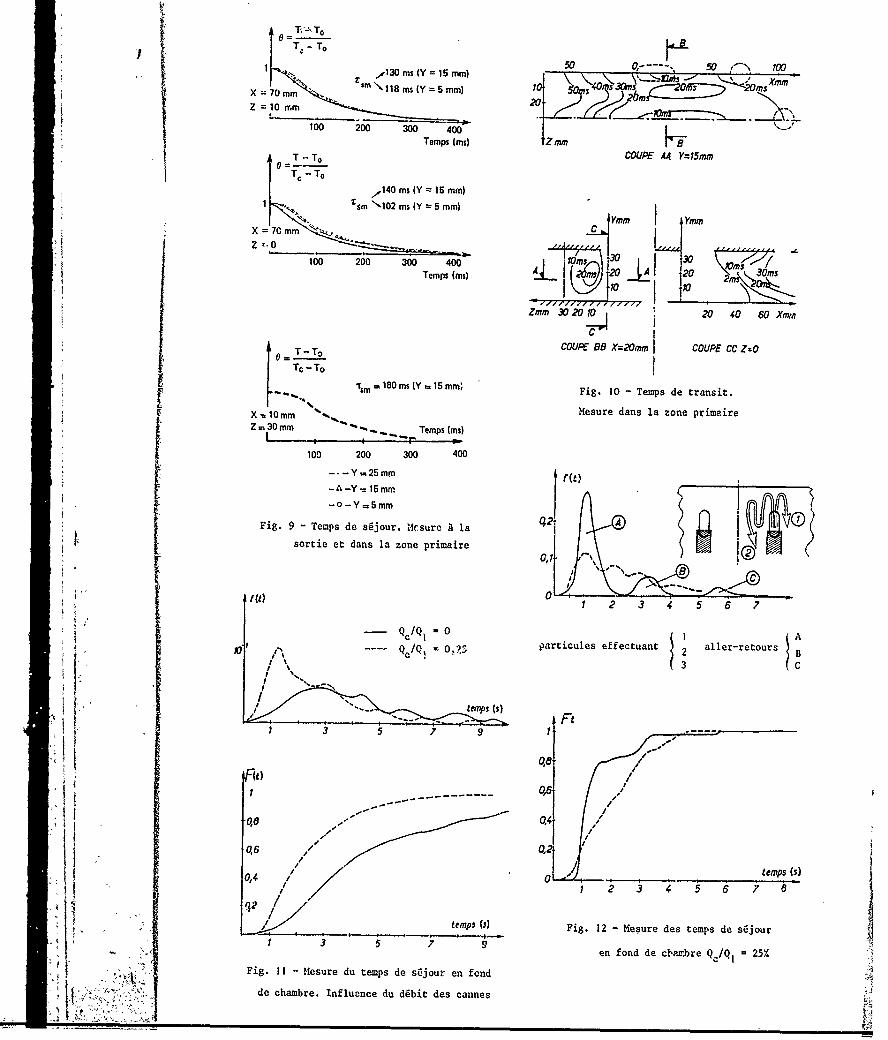
-T c - T,

50 50 'N 100

W ,,140 ms (Y = 15 ram) 0 Ss M

7 mm 118 ms (Y = 5 mm)0

Z= Ismm =5m)10Zmm032000Temp20ms0 60

T T COUPE AA Y15mm

Te - T,r 140 ms (Y = 15 mm)

1 .T sm O2 ms (Y=5 mm) j m I Ym

i X70Omm 70ur mmn lazoeprm, r

Z 0Temps(ms)

100 200 300 400 1 3ms20 271 K 3 0ms20 2 0

Zmm 30 200 0

COUPE BB X=2Omm I COUPE CC ZZO

TC - T

1o-Y= ms Y15m,

T Sm d s . s Fig. 10 - Temps de transit.

X o 10mm eMesure dans la zone primireZ=.30Omm ... -~ Temps (ms)

100 200 300 400

-Y 15 mmI-0- Y.5mm I{Fig. 9 - Temps de s~jour. ilcsure A la A

sortie et dans la zone primaire0,71 '

t)1 2 34 5 6 7

Qc/Q, . 0 articules effectuant aller-retours A

% 3 C

0,6 046s

0,6 02 i

0o4 /i tem__ . __ _ , ps (5)2 3 4 57 8

7 9

0 ,empi (s) Fig. 12 - Mesure des temps de s=jour

3 5- \-'en fond de cbpz~bre- QOC/Qi 25%".

Fig. II - Hesure du temps de s6jour en fend

de chambre. Influence du debit des cannes

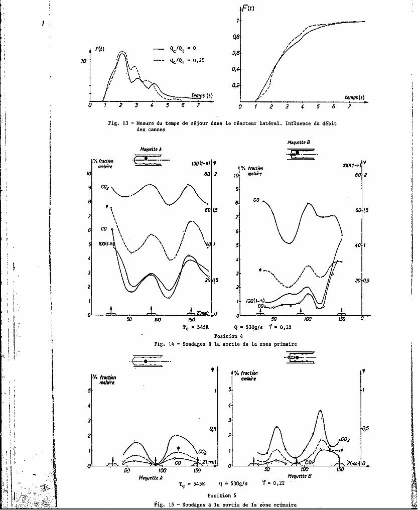
101 1 Qd/Qi =0,25j I0,/

0,2

/ -, emp 3(S)

0 1 2 3 4 5 6 70 1 2 3 4 5 6 7

Fig. 13 -Mesure du temps de sfijour dans le rdacteur latfiral. Influence du dibitdes cannes

Maqwtte BMaqtft A -

10 8002 1 molaire 80 2

9 CO.. 9

9'601,56 ,

6 CO 'I \6

5100(1-1 V 1

33/

2 2

Te -55 39sY-0,22

Fig.14 ondaes la orte dela oneprimaire

% fr~c~on " friction 4mere onlere

44

3 1I, 0,5 ,5

2 2

1 ~c 2 1- 0 1*- \%

0[ 01Maquete AMaquette B

TeSS Q 530g/s 'f0,22

Position 5Fig. 15 -Sondages a la sortie de fa zbue orimaire -

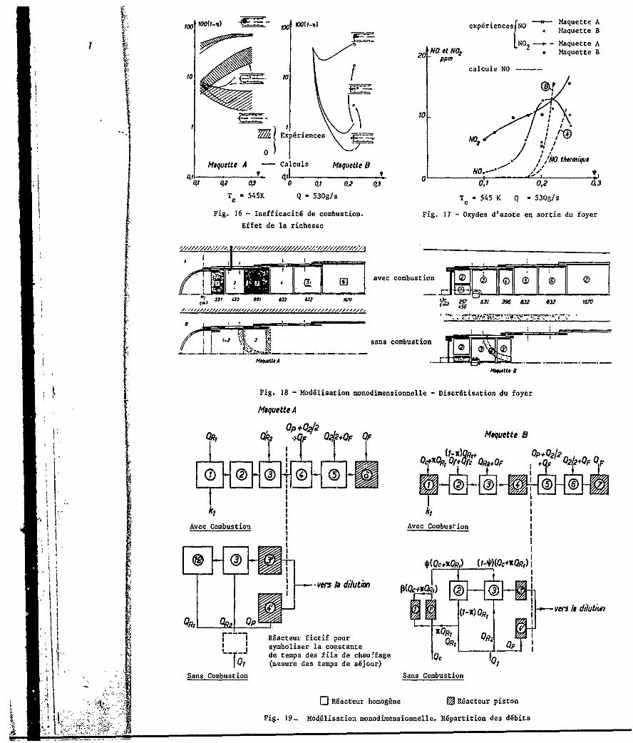
too 100-14) 1000(-11) exdine O~ Maquette Ax2 Maquette B

[NO --- MaquetteANO ot A(02 2 Maquette B

& [calculs NO - -

Expfriences A10 Z "

Maquefte A - Calcuis Maquette B -. ~ ii hri0,1 (III v 01________ NO.-' p

01 42 -01 o 0,2 03 0, 2 0,3

T e -545K Q -53g/s Te .-545 K Q -530g/s

Fig. 16 - Inefficacitfi de combustion. Fig. 17 -Oxydes d'azote en sortie du foyer

Effet de la richesse

Savec combus tion

J21 42,1 061 In W32 1 61).V 3,. ,, / //CM,,, , 456

Jsans combustion iF J T

Fig. 18 -Mod~iiaation monodimensionnelle -Discr~tisation du foyer

Maquette A

lop + QJ/2OR, Ok# OF Q* O F Maquette B

2 4

Avec Combustion AvcCmuto

+$Qci.KQR) (1-0)(cXQ1g) I

H veu /a dilution

I~~XR 1 yblsri

de L..f.J des fl eca 0

Sans Combustion dsSans Combustion

j Ii RUalteur homog~ne R~acteur piston

h Fig. 19.. Mod,61isatioa monodiniensionneile. Rdpartition des ddbits

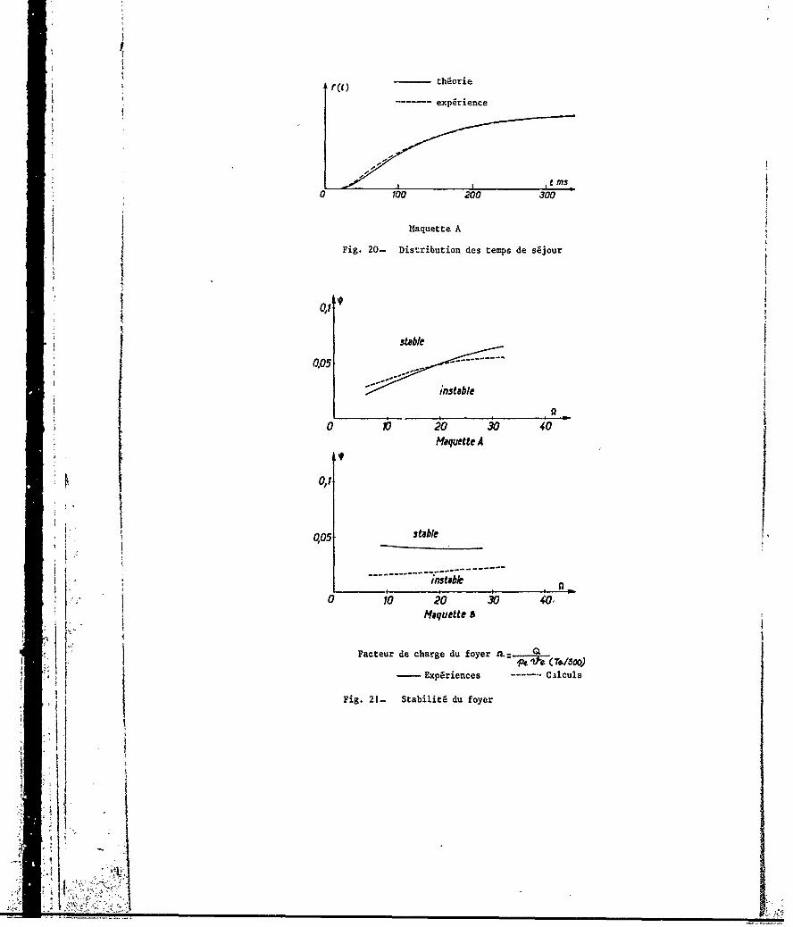
exp~rience

0 100 20300

Maquette, A

IFig. 20- Distribution des temps de s~jour

I 0,7stable

L005. -----

-- instable

0 Pl~aquette A300

0,1

0,05 stable

--------------- --------------

instable

0 10 20 30 40,Maquette a

I'Facteur de charge du foyer Q:

- xp 6riences --- *C1lculs

Fig. 21- Stabiliti dui foyer

DISCUSSION

D.C.Dryburgh, USI would like to link this paper with Professor Odgers' paper and the remarks I was making in defence of complexmodels. I was very delighted by these beautiful flow visualisations. Tie remark I would really like to make, is thatif you have got a good aerodynamic model that will reproduce these results you can use that model to quantify thepictures that we got. We saw, that when you injected the dye into different points in a particular hole the flowwent in different places; it behaves in completely different ways. If you can simulate that in a model and storethe results you can do all sorts of things with such results. You can use it to predict your residence times, to fit into the other plug flow and mixed reactors that you used. You can use a complex model as a starting point for allsorts of calculations. You can do the flow visualisation in great detail. If you have got the right sort of computordisplay facilities, you can look at your film from different points of view and use it to give people a good under-standing of what is going on in the combustion chamber. It is one of the great attraction of a complex flow model.The other statement I would like to point out is that these models very often have to be done cold. Our experiencehas been that although the flow may not appear to change very greatly, when you light up a flame, there are somequite important changes which you obviously cannot predict by any flow visualisation techniques. So, I feel thereare limitations to the use of water analogy.

Rdponse d'AuteurNous n'avons pas pu prdsenter dans le d6tail les techniques exp6rimentales de visualisation. Le film prdsent6 estqualitatif, mais comme vous avez pu voir, nous tentons aussi de faire de la visualisation quantitative. Pour chaquefilm rdalis6 nous disposons d'enregistrements sur magndtoscope des images video, qui sont ensuite traitdes parordinateur. On peut alors obtenir soit des mesures de temps de sdjour par suivi de particules, par colorimdtrie. I1est aussi pr6vu de faire de la trajectographie.

Nous pensons effectivement qu'il n'est pas possible de montrer l'influence de la combustion. Malgr6 tout, les simula-tions A froid montrent, dans un premier temps et de manidre qualitative, la configuration de l'deoulement. Etd'apr~s notre experience il n'y a pas de diff6rence fondamentale (toujours d'un point de vue qualitatif) entre les casavec ou sans combustion.

* W.Krockow, Ge

Can you please comment on the possible wall influence on the residence time distribution you measured?

Rdponse d'AuteurSLes rsultats pr6sontds sent obtenus sur une demi-maquette. Avant d'effecter des mesures sur cette demi-maquette,

*Ldeux sries de tests on 6t6 effectu6s:

- comparaison, sur une maquette complete et une demi-maquette, des modules et direction des vitesses moyennesdans la zone primaire. Nous n'avons pas vu de diff6rence fondamentale.

* - compzraison 6galement sur les mesures de temps de s6jour moyen et de la fonction distribution de ces temps des6jour. [A aussi pas de diff6rence notable entre les deux experiences.

~Par centre les m~canismes d'interaction entre jets (battements) peuvent 6tre modifids selon qu'ils sent dtudi~s dans

une demi chambre ou une chambre complete.

'lU I .

REPORT DOCUMENTATION PAGE

I.Recipient's Reference 2.Originator's Reference 3. Further Reference 4.Security Classification~of Document

iAGARD-CP-275 ISBN 92-835-0260-4 UNCLASSIFIED

5.Originator Advisory Group for Aerospace Research and DevelopmentNorth Atlantic Treaty Organization7 rue Ancelle, 92200 Neuilly sur Seine, France

6.Title

COMBUSTOR MODELLING

7. Presented at the Propulsion and Energetics Panel 54th(B) Specialists' Meeting, held at

DFVLR, Cologne, Germany, on 3-5 October 1979.

8. Author(s)/Editor(s) 9.Date

Various February 1980

0.Author's/Editor's Address 1l.Pages

Various 392

12.Distribution Statement This document is distributed in accordance with AGARDpolicies and regulations, which are outlined on theOutside Back Covers of all AGARD publications.

13. Keywords/DescriptorsCombustors Evaporation of fluids Flame oscillationsCombustor models Turbulent diffusion flames Furnace performanceFlow in combustors Ignition Combustion in boilersGas kinetics of combustion Spray bars AfterburnersiMixing of gases Flame stabilization Pollutant emissions

V 14.Abstract

These Conference Proceedings contain the 24 papers presented at the AGARD Propulsionand Energetics Panel 54th (B) Specialists' Meeting on 'Combustor Modelling' which washeld in Cologne, Germany, on 3-5 October 1979. The questions and answers after thepresentation of each paper are included.

The Specialists' Meeting was organized into five sessions: Survey (2 papers); BasicPhenomena (I 1 papers which were presented in two parts); Transient Phenomena andInstabilities (2 papers); Furnaces and Boilers (5 papers); and Gas Turbine Combustorsand R/H Systems (4 papers).

The meeting provided a forum during which the different models and methods used inturbine engine research and development could be compared. Even models used in non-aerodynamical circles were discussed.

The aim of the meeting was to provide research scientists with knowledge on realistic typesof combustor models and on experimental conditions under which the theoretical modelsare valid for practice, and to assist manufacturing engineers in the selection of adequatetheoretical models. Whether the meeting achieved the aim will be assessed in a TechnicalLvaluation Report, to be published as AGARD Advisory Report AR-153.

0 0

0 , c IC,

0 .0 ZCNC-.0. o . -.

W U0 00. .0 c 'n~ ~.

4. .0C 0 l:

0~C 0 > d) (1) C-

0o 0 , 0 cn x M

u- 0. . -,-0> Z W t U

OC0 z " ..

do as 0o 0r0

0 0 . 4)c

U E,

00 Cw

- r -- to

zL '0 Y V~ C' 00 o ~ C0D~ 0

0 00~.~ bo (A

0 0 -) 0 CUI-.Z

00 li 0 (.w. wi~ o

CA r .!2 u .0 0 4

Uifl0 0.: U--Ioi 0 00c

A4 0 Q C . ;5Cl- -" CL M 0 .o CL f

C C

<~0. ~ Cm0 CI w

t4alj -/o c*l

000

to o o c

E0 .0 =o - :-

0, ICU: Vi

,4 .2

~.00 -4.h 0 V -co. Cc) .

E' un' E~

o o. 0 0 . o~~

CC. r- -.1 O -:

04 0

-5 U' ~ UC. aC

.1r1

"1 0 0-(o

to. CV

CE 4w,0 0I n(10 CE1

(1. npC 0 U (10 >

C0 >- E o 0 E ,0

U' 0 (1 0 cc

0 CI oa ,, * a IU'o u 0*) 0CoC

MC -c C( a

~~o 0~ -. ~0E0 ' . .0 '0 '0 l~

'0 z .20

t.. CA0. 4 .0 . . 04

CA ~~ 2 Q ( . J-(A 9

-00. '0, -0 4iii~~ 0' 0~E ~ g

U0 Q0 U'0

C ,4 W1

-C. ~

.- or- 10 10 -00-~~~~~C >____________

4K:] H~ co

NATO + OTrAN

NATIONALBUDISTROBUTION CENTRES

7 RU ACELE22ON~iLYURS~NE -AGARD PUBLICATIONSN

EAR~kbde OhodsokofAADpiainathabvadrs Naorgnal derosacbuorAnatsry, uio NLRG

.publica iois-ade taem AA DMmeNain.trghheflo aina Disbto e nft re.Frhrcpe r oeie

FvaiabCe frmteeNetibti o ayb-pihsil irfce or wegitono efencfome eserchEsablisheneltedblw

9232:Chnatlilon ARD wits Bagneuxic Kelae

dounat ib unjr d *nomta Ii Fore ienia-Aiic erelgt 0ainl l'G R

-Phyik've,, 1140eiiiat l l H e rgie RoaEscl0 Phdnia4

'Deencecigen notiri Srvce Att~lun: GR ainlDIgt

Reoiearh.nd Developent DictatMjit'ofN iolDefence NAiikR'ANa

DanisDhenc Research Ineoraario Centre. ox1

Di.cNER4o Avirition) StaitirSare sIL 2 Avnu Spac AdUitrto DiisoNASAr)PO. k2

Z'IItIifdr1ut n R Aufht-n Reportl dotibto andiq de Material

KenoSclTOCKS OFu GADBLATOSN:PLIATINS AGORC~E SHtoUalD BEAE

PURCHAE AGECIES'GREEofChE Dprm ofheoo~ -RItieflche Mireve o lentRE

Helenisa~ c Ar reGnea tfinistry Spac Nactionatln-eric De ec kioogrea'

*585tLAND, Rbador Sq0ar ruHaroiisu tainSae os'S' iiiflid , Oipiiigtdn,, Keent. BRRFR

Reyiginia26Ik 70SaiF~~ t aYCa

Laiigly'FiEngland6

STOCKS F AGof AGLATION-'NDADLIAI pbitirgvihFoiOjR CM SHOLD BIMAD

publisheihf~~ by *AASiintfc nfecnca' ~ cbhe yteafr'aTlikl'foan Iait Spac Icfiit it i'Servc ,Srmifed

PbstOie' Boihnc 875T - irgimia22 16,' USA-,IfdalfiI~iio i~fic e Natmoa Airor Euo'-'''pa'eAe'i'' -- Cft D

'Sprig ie 7505.P~i ,,Fra~nceSt'.Miiyerdby

,~ Teh~kdtitin'and ei rductin Lt- Rl i - fo , ir h c e o ph t o i s o , AG A R D ' d o e t- h o ld in hid th, A G R e i l n m ,tt e u h r o d t r n