20200225 smart balancing of electrical power - matching

Abbreviations Area Control Error (ACE) Electricity Balancing Guideline (EBGL) Frequency Containment Reserves and system inertia (FCR+) Frequency Restauration Reserves (FRR) Imbalance Settlement Period (ISP) International Grid Control Cooperation (IGCC)

Abstract Ongoing negotiations about future European energy markets stagnate due to disagreements

about power balancing. Dutch and Belgian systems count on real-time transparency allowing passive balancing: All market parties are incentivized to balance generation and load in the control area. The German system pursues a strategy relying only on prequalified reserves.

The idea of passive balancing is expanded. A definition of Smart Balancing is proposed. The introduced Smart Balancing indicators evaluate market performance by scaling a) the demand for power balancing and b) resulting costs. Applied data cover a five-year time period (2015 to 2019). The results show that passive balancing is a cost-efficient tool for coping with unscheduled fluctuation between power generation and load. Empirical data suggests that the German strategy is undermined, and passive balancing is present. On the other hand, misplaced incentives intensified four German imbalance events (June 2019) and balancing power of up to 7.5 GW had to be activated.

The findings lead to policy implications. It is concluded that changes in timing schemes of energy and balancing markets are required in the first place. In the German system, transparency and real-time information would improve cost-efficiency of power balancing.

Highlights • Power system requirements and market performance indicators • Transparency and real-time information are key for cost-efficient power balancing • Passive balancing is present in Germany and current market rules are inconsistent • June events in Germany were intensified by misplaced incentives • Policy implications and future European market approach

1. Introduction The European power system evolved from independent island systems to national balancing areas, finally connected to international synchronous grids with high reliability. Harmonization and integration of electrical systems facilitated international trade leading to economic benefits. The objective of current efforts are harmonization and integration of balancing markets (ENTSO-E, 2017). Power balancing ensures the balance between power generation and load. It is subject to both reliability and economic benefits. Therefore, existing power balancing strategies are under

Smart Balancing of electrical power – Matching market rules with system requirements for cost-efficient power balancing

Author: Felix Röben1,2,3

Affiliations 1. Energieberatung Hamburg, enhh.de 2. University of applied sciences HAW Hamburg, CC4E 3. Fraunhofer-Institut für Siliziumtechnologie ISIT Keywords: Power Balancing, Market design, European energy market, Smart Balancing, Passive Balancing

2

consideration. This article aims to contribute to the negotiations about power balancing in future European energy markets. The Dutch and Belgian balancing strategies count on market response for power balancing, also known as passive balancing. For that purpose, real-time information about activated balancing reserves and the current imbalance price are available. All market parties are incentivized to balance generation and load in the control area in addition to prequalified reserves. The German strategy does not provide official real-time information and relies upon on prequalified reserves.

Figure 1: Smart Balancing of electrical power – Method to develop policy implications and future market rules

Figure 1 shows the structure of the article at hand. Physical constraints, market rules and related system services of electricity supply are introduced in section 2. Section 3 provides a definition of Smart Balancing and introduces the Smart Balancing indicators. Section 4 presents three case studies and outlines the performance of the Netherlands, Belgium and Germany over a five-year period from 2015 to 2019. Section 5 discusses the results and thus evaluates the considered balancing strategies. Section 6 concludes on policy implications and an approach for the future European energy market is outlined.

2. Power system requirements, imbalance netting and market rules Matching market rules with system requirements is crucial for reliable and cost-efficient electricity supply. Therefore, physical constraints and system services (2.1), the concept of imbalance netting (2.2) and current market rules (2.3) are outlined.

2.1. Physical constraints and system services for reliable electricity supply Physical constraints must be addressed by fail-safe measures to ensure reliable electricity supply. Figure 2 illustrates the two considered physical constraints. A. Frequency stability and B. grid capacity. The vertical axis illustrates weather the constraint occurs globally in the synchronous zone or locally in a transmission line. C. Power balancing influences both physical constraints and is organized within control areas.

Power system requirements

Policy Implications

Market rules and system services

Future European market

Smart Balancingindicators

Evaluate balancing strategies

Data from countries

Data Analysis / Case Studies

content

spec

ific

gene

ric

Section 2

3

4

5

Section 6

3

Figure 2: Physical constraints and resulting system services for a reliable electricity supply

A: The frequency is the physical quantity which defines a synchronous zone. Any power deviation between infeed and withdrawal impacts the global frequency. It is an indicator for the balance between all generation and load of the synchronous zone. Deviations from the set-point frequency are minimized by 3 GW of Frequency Containment Reserves in central Europe (ENTSO-E, 2009). In addition to the frequency itself, also a high rate of change of frequency (ROCOF) must be kept within limits. Frequency stability is therefore obtained by the combination of Frequency Containment Reserves and system inertia (FCR+) (Dreidy et al., 2017). B: The grid capacity is a local physical constraint. The maximum power flow through a transmission line must not be exceeded. Either curtailment reduces the local power generation or (temporary) market splitting increases power consumption. Both measures can relive the grid until the required capacity expansion is completed (Håberg et al., 2019). C: Power balancing within control areas is a mechanism which interacts with the two described physical constraints. Power balancing is not based on a physical constraint, but on international agreements and national legislation. Regardless of details, power balancing assets: A. Support frequency stability of the synchronous zone. B. Limit unscheduled power flows between control areas. These assets are prequalified Frequency Restauration Reserves (FRR). The control variable is the area control error (ACE), described by Equation 1. The ACE is the deviation between the sum of all scheduled power flows (Pscheduled) and the sum of all measured power flows (Pmeasured) into or out of a control area (ENTSO-E, 2009).

𝐴𝐶𝐸 = ∑𝑃!"#$%&'$% − ∑𝑃($)!&*$% (Equation 1)

The three system services follow different control variables and, thus, counter-activations can occur. A. FCR+ responds to the global frequency; B. measures to relive the grid react to the local power flow in transmission lines; C. activation of FRR reacts to the ACE in a control area.

2.2. Imbalance netting The International Grid Control Cooperation (IGCC) on imbalance netting help avoiding unnecessary counter-activation of FRR in neighboring control areas. Imbalance netting is applied, if the ACE of two neighboring control areas have different signs (positive ACE vs. negative ACE). Thus, IGCC saves cost on both sides. The activation of FRR is reduced by allowing unscheduled power flows between control areas. This mechanism requires available cross-zonal grid capacity (ENTSO-E, 2016).

A: Frequency stability

Smart Balancing indicators

Physical constraints and system services

C: Power balancing

FRR and imbalance netting

FCR+

B: Grid capacity Local flexibilityloca

lgl

obal Synchronous zone

Control area

Transmission line / node

4

2.3. Current market rules in the Netherlands, Belgium and Germany Market rules developed historically, e.g. with national power generation characteristics. Heterogenous legislations are in place. The future European market is partly directed by the EU winter package 2017. The “Electricity Balancing Guideline” (EBGL) harmonizes market design and balancing mechanisms in all EU countries (ENTSO-E, 2017).

Figure 3: Market rules and balancing strategies in Germany (GER) vs. balancing in the Netherlands (NL) and Belgium (BEL)

Figure 3 illustrates the timing of current markets in Germany. Timing details of markets in the Netherlands and Belgium differ, but are subject to short-term harmonization (Röben, 2018). The box over the timeline represents “energy-only” markets. Buy and Sell orders for energy are the main tool to coordinate generation and load of electrical power. Continuous trade at intraday markets and changing the schedule is possible until 15 minutes before real-time (M-15) in Germany (Bundesnetzagentur, 2011). The boxes under the timeline are related to power balancing. Market parties offer prequalified reserves at balancing markets day-ahead (D-1). All bids at balancing markets build up to cost-optimized merit order lists. Cheaper FRR bids are activated first. Schedule deviations (imbalance of market parties) are cleared with the imbalance price. In all three countries, the average ACE over 15 minutes defines weather a positive or a negative schedule deviation leads to costs or to revenues. The imbalance price is derived from the costs for FRR. Therefore, financial incentives for passive balancing exist in all three countries. Balancing process: Differences can be found in the balancing strategy and imbalance clearing mechanisms. The Netherlands and Belgium apply dual imbalance pricing and publish the imbalance prices to incentivize passive balancing. The dual imbalance price allows to limit market response by allocating different incentives to market parties with positive and negative schedule deviations. Germany applies a single imbalance price. Limiting market response is more difficult with this clearing mechanism, because market parties with positive and negative schedule deviations react to the same incentive. This means a strong financial incentive for passive balancing exist. On the other hand, Germany obligates all market parties to stick to the submitted schedule and thus creates a paradox (legal obligation vs. financial incentive) for them (Röben and de Haan, 2019).

“energy-only” markets: Day-Ahead and Intra-Day

D-1 until M-15 “Real-time” ClearingBalancing power

marketsBalancing Process

Costs / revenues for imbalance

Submission of schedule

t

50 HzfCE

0

PBal

1 GW

Balancing power only (GER) Real-time price incentives (NL, BEL)VS.

5

The official balancing strategies differ, but two recent studies indicate that passive balancing is also present in Germany: (i) Prices at intra-day markets corelate with the most recent (30 minutes delay) information about the German ACE. The authors concluded that market parties buy or sell energy at the intra-day market to create profitable schedule deviations. These schedule deviations reduce the (assumed) ACE, but the delay of information can cause overshooting of the system (Koch and Maskosa, 2019). (ii) The presence of four cycles of market response to high imbalance prices over a 4-hour time period is described. A correlation between passive balancing and activation of expensive balancing reserves is assumed (Röben and de Haan, 2019). The hypothesis from (ii) is assessed and tested with empirical data in section 4.1.2.

3. Smart Balancing of electrical power This section introduces a definition of Smart Balancing and the underlying hypothesis. Furthermore, the Smart Balancing indicators are introduced to evaluate the performance of balancing strategies and to test the hypothesis. Limitations of the methodology are described.

3.1. Definition and hypothesis The idea of passive balancing has been described in different sources. The authors use the abbreviations Balance Responsible Parties (BRPs) for market parties, the Netherlands (NL), transmission system operator (TSO) and System Imbalance (SI) for the ACE:

• ”In NL real-time feedback by the TSO on actual market balance position and imbalance price enables BRPs to act on opportunities to arbitrage between imbalance price and their own marginal production price resulting in a reduction of the system imbalance (the marginal price for control energy determines the actual balance energy price for this passive control).“ (p.102) (Nobel, 2016).

• “The imbalance price provides the incentive to BRPs to “passively” balance the system by purposely deviating from the schedule (“self-balancing”).”(p.1048) (Hirth and Ziegenhagen, 2015)

• “BRPs can help the TSO keep the system balanced by intentionally incurring imbalanced positions in the opposite direction of the SI, which can be referred to as ‘‘passive balancing” (p.45) (Brijs et al., 2017).

These descriptions point out that market parties are incentivized by the imbalance price to passively balance the control area. The risks of misplaced incentives or overcompensation and thus counter activation of FRR is not addressed. The following definition of Smart Balancing is proposed to conclude the idea of passive balancing and expand it by these aspects. Definition: Smart Balancing is a set of measures to avoid the activation of FRR by market parties who create schedule deviations. Smart Balancing is incentivized by correct imbalance pricing in combination with public real-time information. Correct pricing does not incentivize overcompensation. The definition of Smart Balancing addresses the activation of FRR and the risk of overcompensation. Passive balancing becomes Smart Balancing, if market parties are always incentivized to reduce FRR activation without overcompensation. The definition leads to the following hypothesis: Correct imbalance pricing and public real-time information for market parties facilitate Smart Balancing and thus reduce the activation of FRR. This leads to more cost-efficient power balancing without loss of reliability.

3.2. Smart Balancing indicators The Smart Balancing indicators (SBindicators) are introduced to measure and compare (1) power balancing demand and (2) cost-efficiency of power balancing strategies in a data-based way. Figure 4 illustrates the interrelation of three relevant datasets. The schedule deviations cause the ACE in first place. Power balancing consists of two mechanisms (see section 2): 1. Activation of FRR within the control area. 2. The imbalance netting contribution.

6

Figure 4: Smart Balancing indicators

The (1) sum of balancing power demand and (2) sum of costs/revenues are scaled to the local annual energy consumption. Power balancing demand grows with the square root of power consumption, because schedule deviations have zero correlation (p.38) (Frunt, 2011). This is why imbalance netting reduces balancing power demand. Equation 2 (Equation 3) is based on the assumption that schedule deviations have zero correlation. The balancing power demand (cost) grow asymptotically to the square root of power consumption.

𝑆𝐵+,%+")-.*,0.1$* =∑3!""4∑3#$%&'&()*(*,,-(.

5∑3)/(01$2,-/(

(Equation 2)

𝑆𝐵+,%+")-.*,".!- =∑ ".!-!""4∑".!-#$%&'&()*(*,,-(.

5∑3)/(01$2,-/(

(Equation 3)

Equation 2 (Equation 3) lose validity with a growing share of fluctuating renewable energy. Weather conditions cause correlations between schedule deviations of market parties with renewable portfolio. This influence is not considered. A higher share of installed capacity of wind and solar based power generation might lead to differences in FRR demand which are not covered. For the sake of comparison, Equation 4 (Equation 5) introduce a worst-case indicator (WCindicator). It is based on the assumption that balancing power demand (cost) grow linear with the power consumption.

𝑊𝐶+,%+")-.*,0.1$* =∑3!""4∑3#$%&'&()*(*,,-(.

∑3)/(01$2,-/( (Equation 4)

𝑊𝐶+,%+")-.*,".!- =∑".!-!""4∑ ".!-#$%&'&()*(*,,-(.

∑3)/(01$2,-/( (Equation 5)

Equation 4 (Equation 5) is not valid, even in a scenario with 100 % fluctuating renewable energy, because schedule deviations at the consumption side remain with zero correlation. Therefore, Equation 2 (Equation 3) is the more accurate approach and considered to be valid.

FRR

Schedule deviations

Imbalance netting

a) Positive imbalance (e.g. outage at consumption side) b) Negative imbalance (e.g. outage of generation plant)

Smart Balancing indicators:(1) Sum of power(2) Sum of costs/revenues Scale to

(square rootof) localeneryconsumption

a) Upward contribution (import power)b) Downward contribution (export power)

a) Upward reserves (e.g. increase of generation)b) Downward reserves (e.g. decrease of generation)

7

3.3. Limitations of Smart Balancing Limitations of “energy-only” markets are not considered. The resolution of energy products is equal to the Imbalance Settlement Period (ISP) of 15 minutes. This simplification facilitates trade but does not cover individual consumption and generation patterns (ramps) in real-time. National characteristics of power generation and consumption might lead to differences in FRR demand which are not covered. Limitations of the copper plate assumption are not considered. It applies when trading at “energy-only” markets or balancing generation and load with balancing power. Limitations of grid capacity in a control area are subject to secondary downstream measures (curtailment or market splitting, see section 2.1) and are not covered.

4. Introduction and discussion of applied data Datasets with power balancing related timeseries from the Netherlands, Belgium and Germany are analyzed. The timeseries have a resolution of 15 minutes and cover a five-year period from 2015 to 2019. The datasets include a) upward and b) downward values of its (1) power and (2) price components, as illustrated in Figure 4. Power values are given in average power over 15 minutes in MW. Price values are given in €/MWh. Resulting costs/revenues are calculated in € (per 15 minutes). A detailed presentation of the available data is provided in a co-submitted data article (see section 8). Case studies of power balancing demand and costs allow to evaluate the impact of market rules. The Smart Balancing indicators are applied in section 4.2.

4.1. Three case studies Three case studies demonstrate the functionality, (misplaced) incentives of current market rules and their influence on power balancing demand and costs. The introduction of real-time price information in Belgium end of August 2019 (Section 4.1.1.). Empirical data suggests passive balancing in Germany (Section 4.1.2.). Four imbalance events with critical situations in Germany in June 2019 (Section 4.1.3.).

4.1.1. Implications of market change in Belgium The Netherlands publish activated FRR together with the imbalance price close to real-time since 2001 (Beune and Nobel, 2001). Belgium on the other hand, only published the activated FRR without price information. The publication of the imbalance price in Belgium was introduced end of August 2019. The imbalance price is now published in a 1-minute resolution together with the activated FRR (Elia Transmission Belgium SA, 2020). In addition, the contribution to IGCC (in MW) and costs/revenues for imbalance netting (in €/MWh) is provided to the market parties. The real-time price publication covers only three months of the applied data, but a comparison of mean costs for power balancing indicates an improvement of cost-efficiency. Table 1 shows mean values of power balancing demand (average power over 15 minutes) and resulting costs (in € per 15 minutes). While FRR demand and imbalance netting contribution remains stable, related costs decrease, especially for imbalance netting (see gray area in Table 1).

8

Table 1: Average imbalance, FRR activation and cost (Elia Transmission Belgium SA, 2020)

Average values over 15 minutes of

01.01. to 31.08.2018

01.09. to 31.12.2018

01.01. to 31.08.2019

01.09. to 31.12.2019

Activated FRR (up and down)

77.5 MW 78.5 MW 76.2 MW 75.3 MW

Costs for FRR (up and down)

1104.1 € 1214.5 € 811.8 € 736.1 €

Imbalance netting via IGCC

48.3 MW 45.7 MW 48.6 MW 47.4 MW

Costs for Imbalance netting

90.9 € 121.1 € 22.4 € 11.3 €

4.1.2. Passive balancing in Germany A previous case study claimed that market parties in Germany react to the activation of mFRR with passive balancing (Röben and de Haan, 2019). This subsection aims to identify such a behavior with empirical data. The mean and median values of the ACE and of the ACE difference to the last ISP are therefore under consideration. Hypothesis: Activation of mFRR leads to passive balancing and, therefore, the ACE difference to the last ISP moves in an ACE reducing direction in case of mFRR activation. Table 2 gives an overview about all ISPs with positive ACE (105952 ISPs or 3 years or 60 % of the time). Table 3 gives an overview about all ISPs with negative ACE (69343 ISPs or 2 years or 40 % of the time). Besides this separation of data by the sign of the ACE, two additional layers of filters are applied in the Tables. Filter by mFRR activation: The second row includes only ISPs with upward (downward) mFRR activation, and the third row includes the ISPs without upward (downward) mFRR activation. Filter by ACE: The second column shows ISPs with ACE over 1 GW (under -1 GW) and the third column shows ISPs with ACE between 1 GW and 1.5 GW (between -1 GW and -1.5 GW). Table 2: ISPs with positive ACE, market response to mFRR activation in Germany, data from 2015 to 2019

Applied filter Positive ACE ACE > 1 GW 1 GW < ACE < 1.5 GW All ISPs Count: 105952

Mean ACE: 405 MW Mean ACE difference: 49 MW

Count: 6313 Mean ACE: 1329 MW Mean ACE difference: 176 MW


ISPs with upward mFRR

Count: 6797 Mean ACE: 985 MW Mean ACE difference: - 148 MW


Count: 1934 (Figure 5: yes) Mean ACE: 1220 MW Mean ACE difference: - 41 MW

ISPs without upward mFRR


Count: 3376 Mean ACE: 1204 MW Mean difference: 311 MW

Count: 3140 (Figure 5: no) Mean ACE: 1157 MW Mean ACE difference: 300 MW

9

Table 2 shows, that the mean ACE difference is smaller in case of upward mFRR activation. Therefore, the ACE tends to move in a favorable direction in case of mFRR activation. The second applied filter (by size of ACE) shows, that this trend is confirmed for smaller datasets only considering ISPs with an ACE over 1 GW. Figure 5 shows boxplots illustrating the median ACE (left) and the median ACE difference (right) in 5074 ISPs with an ACE of over 1 GW and under 1.5 GW. There are 1934 ISPs with upward mFRR activation and 3140 ISPs without upward mFRR activation (related to gray area in Table 2). The mean ACE difference is 341 MW smaller in case of mFRR activation while the mean ACE is 63 MW higher.

Figure 5: ISP with ACE over 1 GW and under 1.5 GW. ACE difference to last ISP (50 hertz et al., 2020)

The results confirm the hypothesis and indicate that mFRR activation leads to passive balancing. Passive balancing in the order of magnitude of 250 MW to 300 MW are present in ISPs with an ACE between 1 GW and 1.5 GW and upward mFRR activation compared to ISPs without upward mFRR activation. Table 3: ISPs with negative ACE, market response to mFRR activation in Germany, data from 2015 to 2019

Applied filter Negative ACE ACE < -1 GW -1 GW > ACE > -1.5 GW All ISPs Count: 69343

Mean ACE: -331 MW Mean ACE difference: -75 MW

Count: 2857 Mean ACE: -1294 MW Mean ACE difference: -231 MW


ISPs with downward mFRR

Count: 3361 Mean ACE: -886 MW Mean ACE difference: 143 MW


Count: 885 (Figure 6: yes) Mean ACE: -1219 MW Mean ACE difference: 18 MW

ISPs without downward mFRR



Count: 1449 (Figure 6: no) Mean ACE: -1164 MW Mean ACE difference: -350 MW

Table 3 shows, that the mean ACE difference is bigger in case of downward mFRR activation. Therefore, the ACE tends to move in a favorable direction in case of mFRR activation. The second applied filter (by size of ACE) shows, that this trend is confirmed for smaller datasets only considering ISPs with an ACE under -1 GW. Figure 6 shows boxplots illustrating the median ACE (left) and the median ACE difference (right) in 2334 ISPs with an ACE of under -1 GW and over -1.5 GW. There are 885 ISPs with mFRR activation and 1449 ISPs without mFRR activation

10

(related to gray area in Table 3). The mean ACE difference is 368 MW bigger in case of mFRR activation while the mean ACE is 55 MW smaller.

Figure 6: ISPs with ACE under -1 GW and over -1.5 GW. ACE difference to last ISP (50 hertz et al., 2020)

The results confirm the hypothesis and indicate that mFRR activation leads to passive balancing. Passive balancing in the order of magnitude of 300 MW to 350 MW are present in ISPs with an ACE between -1 GW and -1.5 GW and downward mFRR activation compared to ISPs without downward mFRR activation.

4.1.3. Case study of critical situations in Germany in June 2019 Four days with severe situations took place in Germany in June 2019 (06.06.2019, 12.06.2019, 25.06.2019 and 29.06.2019). The activated reserves and misplaced incentives in Germany during the 12.06.2019 are analyzed in this subsection. All available FRR and additional emergency reserves were activated during these events. The events are particularly especial not only because of activated reserves of up to 7.5 GW (12.06.2019). Balancing markets take place day-ahead and define the maximum imbalance price before start of continuous intra-day trade (section 2.3). Continuous intra-day trade leads to fluctuating prices. The prices reflect forecast errors of load and weather predictions. The four critical days are characterized by wind forecast errors (TenneT TSO GmbH, 2019). The intra-day market reflected these corrections with high energy prices. While this is the purpose of intra-day markets, the already defined maximum imbalance price than led to a misplaced incentive for market parties. The penalty for not delivering power (which is the imbalance price) was, therefore, lower than the price at the intra-day market.

11

Figure 7: Critical imbalance, imbalance price and intraday market price in Germany, 12. June 2019 (www.regelleistung.net and www.epexspot.com)

Figure 7 illustrates all activated reserves in Germany, the imbalance price, the intra-day price (high and weighted average) at the 12. June 2019 between 7 am and 5 pm. The highest price at the intra-day market and, during the peak of the imbalance event, even the weighted average price exceeded the imbalance price. The weighted average price is calculated by considering the price of all trades weighted by the traded energy volume. Market parties could therefore generate revenues by selling energy and not delivering. Also, market parties with forecast errors are incentivized to pay the imbalance price rather than correcting their schedule at the intra-day market.

0

200

400

600

800

1000

1200

0

1500

3000

4500

6000

7500

7:00

8:00

9:00

10:0

0

11:0

0

12:0

0

13:0

0

14:0

0

15:0

0

16:0

0

imba

lanc

e pr

ice, i

ntra

-day

pric

e: h

igh

and

wei

ghte

d av

erag

e in

€/M

Wh

aFRR

+ m

FRR

+ em

erge

ncy

rese

rves

. in

MW

Germany: misplaced incentive 12.06.2019

aFRR + mFRR + emergency reserves

moving average

imbalance price

intra-day price: high

intra-day price: weighted average

12

4.2. Data analysis with Smart Balancing indicators The Smart Balancing indicators (see section 3) are applied to the datasets (of the Netherlands, Belgium and Germany over a five-year period from 2015 to 2019). Table 4 shows the annual energy consumption in GWh, required for scaling and thus comparison of the three countries. The mean power consumption µ in GW is given for comparison. The values are derived from 15-min average energy consumption (sum up and calculate mean). Table 4: Energy consumption in the Netherlands, Belgium and Germany (ENTSO-E Transparency Platform, 2020)

Netherlands (NL) Belgium (BEL) Germany (GER)

Energy consumption

2015 97 749 GWh µ = 11.2 GW

87 998 GWh µ = 10.0 GW

477 924 GWh µ = 54.6 GW

2016 114 004 GWh µ = 13.0 GW

86 886 GWh µ = 9.9 GW

481 084 GWh µ = 54.8 GW

2017 113 835 GWh µ = 13.0 GW

87 313 GWh µ = 10.0 GW

477 924 GWh µ = 56.3 GW

2018 114 721 GWh µ = 13.1 GW

87 487 GWh µ = 10.0 GW

508 535 GWh µ = 58.1 GW

2019 103 128 GWh µ = 11.8 GW

84 949 GWh µ = 9.7 GW

484 895 GWh µ = 55.4 GW

Table 5 shows demand and costs of FRR and of IGCC before scaling. Energy values are derived from 15-min average power values (calculate energy and sum up). Costs are derived from 15-min average power values multiplied with average price values (calculate costs and sum up). Table 5: FRR and IGCC power demand and costs/revenues – data from (TenneT Holding B.V., 2019), (Elia Transmission Belgium SA, 2020), (50 hertz et al., 2020)

Netherlands (NL) Belgium (BEL) Germany (GER)

FRR(up and down) 2015 516 GWh 35.00 mio. €

751 GWh 35.69 mio. €

2 810 GWh 98.55 mio. €

2016 452 GWh 23.25 mio. €

629 GWh 24.65 mio. €

2 348 GWh 84.04 mio. €

2017 513 GWh 28.42 mio. €

639 GWh 24.79 mio. €

2 428 GWh 107.10 mio. €

2018 619 GWh 44.01 mio. €

686 GWh 42.46 mio. €

2 520 GWh 117.86 mio €

2019 559 GWh 38.68 mio. €

661 GWh 26.35 mio. €

2 649 GWh 105.00 mio. €

IGCC(im- and export) 2015 420 GWh 7.79 mio. €

255 GWh 4.09 mio. €

977 GWh 20.59 mio. €

2016 637 GWh 8.00 mio. €

428 GWh -0.55 mio. €

1 434 GWh 33.24 mio. €

2017 632 GWh -0.47 mio. €

427 GWh 1.82 mio. €

1 056 GWh 29.12 mio. €

2018 598 GWh 2.48 mio. €

401 GWh 4.07 mio. €

1 277 GWh 32.54 mio. €

2019 654 GWh -0.66 mio. €

411 GWh 0.36 mio. €

1 224 GWh 17.62 mio. €

13

Table 6 shows the resulting Smart Balancing indicators (data in Table 4 and Table 5, Equations in section 3.2). Demand and costs of FRR and IGCC are added and scaled to the square root of the local energy consumption. Table 6: Smart Balancing indicators with data from Table 4 and Table 5

Smart Balancing indicators Netherlands (NL) Belgium (BEL) Germany (GER)

SBindicators (Equation 2 and Equation 3)

2015 3.0 !"#√!"#&'().

136.9 +€√!"#&'().

3.4 !"#√!"#&'().

134.1 +€√!"#&'().

5.5 !"#√!"#&'().

172.3 +€√!"#&'().

2016 3.2 !"#√!"#&'().

92.5 +€√!"#&'().

3.6 !"#√!"#&'().

81.8 +€√!"#&'().

5.5 !"#√!"#&'().

169.1 +€√!"#&'().

2017 3.4 !"#√!"#&'().

82.9 +€√!"#&'().

3.6 !"#√!"#&'().

105.9 +€√!"#&'().

5.0 !"#√!"#&'().

197.0 +€√!"#&'().

2018 3.6 !"#√!"#&'().

137.2 +€√!"#&'().

3.7 !"#√!"#&'().

157.3 +€√!"#&'().

5.3 !"#√!"#&'().

210.9 +€√!"#&'().

2019 3.8 !"#√!"#&'().

118.4 +€√!"#&'().

3.7 !"#√!"#&'().

91.6 +€√!"#&'().

5.6 !"#√!"#&'().

176.1 +€√!"#&'().

Figure 8 illustrates the Smart Balancing indicators of the Netherlands, Belgium and Germany over time. Both indicators show the Netherlands and Belgium have a similar power balancing performance. Germany has higher scaled power balancing demand and higher scaled costs than the Netherlands and Belgium.

Figure 8: Smart Balancing indicators (power demand left and costs right) with data from Table 4 and Table 5

14

Table 7 shows the resulting worst-case indicators (data in Table 4 and Table 5, Equations in section 3.2). Demand and costs of FRR and IGCC are added and scaled to the local energy consumption. Table 7: Worst-case indicators with data from Table 4 and Table 5

Worst-case indicators Netherlands (NL) Belgium (BEL) Germany (GER)

WCindicators (Equation 4 and Equation 5)

2015 9.6 -"#!"#&'().

438 €!"#&'().

11. 4 -"#!"#&'().

452 €!"#&'().

7. 9 -"#!"#&'().

249 €!"#&'().

2016 9.6 -"#

!"#&'().

274 €!"#&'().

12.2 -"#!"#&'().

277 €!"#&'().

7. 9 -"#!"#&'().

244 €!"#&'().

2017 10.1 -"#

!"#&'().

246 €!"#&'().

12. 2 -"#!"#&'().

358 €!"#&'().

7.3 -"#!"#&'().

285 €!"#&'().

2018 10. 6 -"#

!"#&'().

405 €!"#&'().

12.4 -"#!"#&'().

531 €!"#&'().

7.5 -"#!"#&'().

296 €!"#&'().

2019 11. 8 -"#

!"#&'().

369 €!"#&'().

12.6 -"#!"#&'().

314 €!"#&'().

8.0 -"#!"#&'().

253 €!"#&'().

Figure 9 illustrates the worst-case indicators of the Netherlands, Belgium and Germany over time. The worst-case indicator for power demand confirms that scaling to energy consumption without square root give an advantage to countries with high energy consumption. The smallest balancing demand is found in the country with highest energy consumption and vice versa. The worst-case indicator for costs, on the other hand, show a remarkable year. The Netherlands had lower costs in 2017. This can be attributed to moderate costs for FRR and revenues from imbalance netting via IGCC, as shown in Table 5. Similar to the findings in section 4.1.1 (Belgian case), imbalance netting via IGCC contributes to the cost-efficiency of the Netherlands in this case, as well.

Figure 9: Worst-case indicators (power demand left and costs right) with data from Table 4 and Table 5

15

5. Results and Discussion The three considered countries (the Netherlands, Belgium and Germany) apply two different balancing strategies. The strategies differ mainly in transparency to incentivize efficient passive balancing with real-time information. The transparent approach is found in the Netherlands and Belgium. Publication of data on current imbalance volumes and prices close to real-time is visible online to the general public. Schedule deviations are allowed, and any market party is encouraged to act in favor of system stability. Dual imbalance pricing allows to control and limit passive balancing by choosing different incentives for market parties with positive or negative schedule deviations. Existing definitions of passive balancing are expanded, and a definition of Smart Balancing is derived (section 3.1). The German balancing market design does not include transparent incentives for market parties other than keeping to their submitted schedule. Information on imbalance volumes and prices is only published ex post. The German strategy is to minimize imbalances by promoting good scheduling (accurate load and generation prediction). The strategy foresees to compensate any imbalances by the activation of balancing power. On the other hand, a single imbalance price is applied which rewards market parties who perform passive balancing. The literature does not provide indicators for comparing the performance of power balancing in control areas with different energy consumption. Therefore, Smart Balancing indicators are introduced (section 3.2) to measure market performance by evaluating a) the demand for power balancing and b) resulting costs. The Smart Balancing indicators show which countries have been performing best over the period from 2015 to 2019 when it comes to cost-efficient power balancing (section 4.2). The Netherlands have the best performance, followed by Belgium. Outstanding are the low costs, or even revenues, for imbalance netting contribution in the Netherlands and Belgium compared to moderate costs in Germany. Transparency about the imbalance netting contribution in combination with the imbalance price leads to cross-zonal passive balancing. Therefore, passive balancing in the Netherlands and Belgium help to balance neighboring control blocks (such as Germany) and improve cost-efficiency on both sides. The results imply that transparency improves cost-efficiency of power balancing. These findings go along with the hypothesis that real-time information about system imbalance and imbalance price are key for cost-efficient power balancing. The introduction of transparency in Germany could, therefore, improve power balancing. Findings in previous research came to similar results.

• Hirth and Ziegenhagen (2015, p. 1048) state: “Fostering passive balancing could be an alternative (indeed, a very good substitute) to the introduction of energy- only balancing markets.”

• Nobel (2016, p.109) argues: “Provision of balancing energy by the system operator is a result, and not the objective of power balancing. This choice allows, invites, and basically incentivizes active participation and competition between imbalance and balancing energy.”

• Brijs et al. (2017, p. 49) conclude: “as passive balancing can serve a valuable social purpose and improve the valorization of flexibility, incentivizing design changes should be considered for the French and German balancing markets.”

Furthermore, three case studies are carried out to identify existing (misplaced) incentives in current market rules. Introduction of a public imbalance price in Belgium end of August 2019 shows that no unexpected market (over-) reactions took place (section 4.1.1). While power balancing demand remained stable, the cost-efficiency was improved. The considered time period with real-time price information covers only three months. Nevertheless, the Belgian case suggests that the practice of publishing not only the imbalance, but also the imbalance price is the more efficient approach of incentivizing passive balancing of market parties. The presence of passive balancing in Germany as response to high imbalance prices is analyzed (section 4.1.2). The data indicates that the German strategy is undermined and the existing financial incentive to perform passive balancing leads to temporary market response. Any

16

information, like the activation of mFRR, are used to predict the imbalance price. This practice carries the risk of overreaction. An imbalance to the opposite direction can result, because market parties do not get any official information or any other kind of feedback on their behavior. The four imbalance events in June 2019 in Germany illustrate a misplaced incentive for market parties (section 4.1.3). The intraday market price exceeded the imbalance price. Therefore, to correct forecast errors (by buying energy at the intraday market) was more expansive than not delivering and paying the imbalance price. Even worse: Market parties were incentivized to sell energy without the capacity to deliver (“Short sales of energy”). The high spread between intraday market price and imbalance price made system threatening behavior profitable. The imbalance price could be estimated by market parties, because the merit order list for balancing reserves is published day-ahead. The events in June require rethinking the timing schemes of current market rules. Incentivizing short sales of energy must be avoided. Correction of forecast errors at intraday markets must be rewarded. The European Commission mandates the answer in the GLEB, article 24.2: “Balancing energy gate closure times shall: (a) be as close as possible to real-time; (b) not be before the intraday cross-zonal gate closure time; (c) ensure sufficient time for the necessary balancing process” (ENTSO-E, 2017). By adjusting the timing schemes accordingly, reliable flexibility would be available at short term intraday markets. Wrong scheduling can still lead to high prices at the intraday market, but the balancing energy bids at balancing markets are submitted after gate closure of the intraday market. The imbalance price will, therefore, increase over the market price in case of a (short) system imbalance, because only expansive reserves remain for the balancing market. Short sales at the intraday market are not incentivized.

6. Conclusion and Policy Implications Smart Balancing is defined to comply with physical system requirements and improve cost-efficiency of power balancing mechanisms. The balancing strategies in the Netherlands and Belgium allow passive balancing: Market parties generate revenues with schedule deviations which reduce the imbalance between generation and load in the country. The applied dual imbalance prices allow to control and limit overcompensation by allocating separate prices to market parties with positive and negative schedule deviations. Thus, the two countries fulfill the Smart Balancing requirements. Germany, on the other hand, has inconsistent market rules: Real-time information is missing, but passive balancing is rewarded by a single imbalance price. Even though the German balancing strategy does not allow schedule deviations, the financial incentive to perform passive balancing is, therefore, stronger than in the other two countries. This explains, why empirical data suggests that passive balancing is present in Germany. Apparently, market parties respond to uncertain information (activation of expensive mFRR). There is no option to limit or control their behavior in the current German system. The power balancing performance indicates that transparency and real-time information reduce the activation of balancing power and improve cost-efficiency. Remarkable is Smart Balancing with imbalance netting via IGCC, because market parties in the Netherlands and Belgium make profit by supporting power balancing in Germany. In the context of harmonization, the German power balancing strategy should therefore converge towards the strategy in the Netherlands and Belgium. Figure 10 shows opportunities and information for market parties with current market rules on a timeline. The case study about four imbalance events in June 2019 in Germany (activated balancing reserves of up to 7.5 GW) lead to policy implications regarding timing schemes in the Netherlands, Belgium and Germany. In the three countries, balancing markets take place day-ahead and the imbalance price can therefore not reflect (weather or demand) forecast errors. In the German cases in June 2019, correction of weather forecast led to misplaced incentives. The intraday “energy only” market price increased over the imbalance price. Therefore, correction of

17

forecast errors at the intraday market was more expansive than paying the imbalance price. Selling energy without delivery led to revenues. Changes in timing schemes are required to avoid this kind of misplaced incentives.

Figure 10: Current market rules in the Netherlands (NL), Belgium (BEL) and Germany (GER)

In Germany, Smart Balancing can be achieved by a set of measures. In the Netherlands, Belgium and Germany, changing timing schemes can replace misplaced incentives of current market rules. The proposals in Table 8 are recommended for national policy makers to achieve Smart Balancing in Germany and avoid misplaced incentives in all three countries. It goes along with the European legislation, namely the EBGL (ENTSO-E, 2017). Table 8: Current market rules and proposals for policy changes

Current market rules Proposal

Netherlands, Belgium and Germany.

Timing of balancing markets (Day-ahead) and “energy-only” markets (intraday) can lead to misplaced incentives (e.g. during the “June events”).

Gate-closure time of balancing markets after “energy-only” markets and close to start of ISP.

Germany The imbalance price incentivizes passive balancing, which is not allowed. Lacking transparency and uncomplete information could lead to over-reactions of market parties.

Introduction of real-time information for market parties to incentivize passive balancing. Introduction of dual imbalance price to limit and control over-reactions.

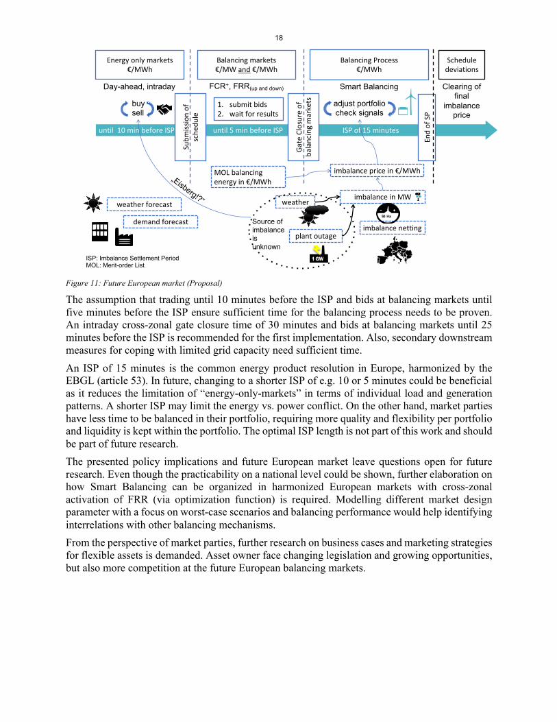
Figure 11 shows the timeline of opportunities and information in the future European market, after harmonization with the proposed policy changes in Table 8. The intraday trade and submission of the final schedules take place before the gate closure of balancing markets. The proposed timing scheme ensures that the imbalance price will always exceed the intraday market price in case of activation of positive balancing reserves. Therefore, to correct forecast errors at the intraday market is beneficial compared to paying the imbalance price. Short sales do not lead to profit.

Balancing markets€/MW and €/MWh

Energy only markets€/MWh

Schedule deviations

Day before ISP until 15 min before ISP ISP of 15 minutes

weather forecast

Balancing Process€/MWh

Gate

Clo

sure

of

bala

ncin

g m

arke

ts

Current market rules

buysell

FCR, FRR(up and down)

demand forecastSu

bmiss

ion

of

sche

dule

Day-ahead, intraday

End

of S

P

Different strategies

Balancing power only (GER) vs. real-time price

incentives (NL, BEL)

Clearing of final

imbalance price

1. submit bids2. wait for results

imbalance nettingplant outage

weather

imbalance price in €/MWh

imbalance in MW

MOL of balancing energy in €/MWh

Source ofimbalanceisunknown

ISP: Imbalance Settlement PeriodMOL: Merit-order List

Transparency?

18

Figure 11: Future European market (Proposal)

The assumption that trading until 10 minutes before the ISP and bids at balancing markets until five minutes before the ISP ensure sufficient time for the balancing process needs to be proven. An intraday cross-zonal gate closure time of 30 minutes and bids at balancing markets until 25 minutes before the ISP is recommended for the first implementation. Also, secondary downstream measures for coping with limited grid capacity need sufficient time. An ISP of 15 minutes is the common energy product resolution in Europe, harmonized by the EBGL (article 53). In future, changing to a shorter ISP of e.g. 10 or 5 minutes could be beneficial as it reduces the limitation of “energy-only-markets” in terms of individual load and generation patterns. A shorter ISP may limit the energy vs. power conflict. On the other hand, market parties have less time to be balanced in their portfolio, requiring more quality and flexibility per portfolio and liquidity is kept within the portfolio. The optimal ISP length is not part of this work and should be part of future research. The presented policy implications and future European market leave questions open for future research. Even though the practicability on a national level could be shown, further elaboration on how Smart Balancing can be organized in harmonized European markets with cross-zonal activation of FRR (via optimization function) is required. Modelling different market design parameter with a focus on worst-case scenarios and balancing performance would help identifying interrelations with other balancing mechanisms. From the perspective of market parties, further research on business cases and marketing strategies for flexible assets is demanded. Asset owner face changing legislation and growing opportunities, but also more competition at the future European balancing markets.

Energy only markets€/MWh

Balancing markets€/MW and €/MWh

Schedule deviations

until 10 min before ISP until 5 min before ISP ISP of 15 minutes

Balancing Process€/MWh

Subm

issio

n of

sc

hedu

le

Future European market approach

buysell

Day-ahead, intraday

Gate

Clo

sure

of

bala

ncin

g m

arke

ts

FCR+, FRR(up and down)

End

of S

P

adjust portfoliocheck signals

Smart Balancing Clearing of final

imbalance price

1. submit bids2. wait for results

imbalance nettingplant outage

weather

imbalance price in €/MWh

imbalance in MW

MOL balancing energy in €/MWh„Eisberg!?“

Source ofimbalanceisunknown

ISP: Imbalance Settlement PeriodMOL: Merit-order List

weather forecast

demand forecast

19

Acknowledgements I would like to thank Prof. Dr. Clemens Jauch, Prof. Dr. Jens-Eric von Düsterlho, Dr. Jerom E. S. de Haan and Henning Thiesen for providing help during the research with proof reading the article.

7. Data availability The considered energy consumption time series were obtained from the ENTSO-E Transparency Platform (https://transparency.entsoe.eu/). The power and price components for FRR were obtained from the homepages of the system operators (Netherlands: www.tennet.org, Belgian: www.elia.be, Germany: www.regelleistung.net). The power and price components for imbalance netting via IGCC were obtained from the homepage of the German system operators (www.regelleistung.net). All cost time series were calculated. The unique cost time series created for this article are subject of a co-submitted data article, which shows more details. The intraday energy prices during the German imbalance events in June 2019 were obtained from the homepage of epexspot (www.epexspot.com).

8. References 50 hertz, Amprion, TenneT, Transnet BW, 2020. Internetplattform zur Vergabe von Regelleistung. URL https://www.regelleistung.net/ Beune, R.J.L., Nobel, F., 2001. System Balancing In The Netherlands. Methods Secure Peak Load Capacity Deregulated Electr. Mark. Mark. Des. Saltsjöbaden 47–58. Brijs, T., De Jonghe, C., Hobbs, B.F., Belmans, R., 2017. Interactions between the design of short-term electricity markets in the CWE region and power system flexibility. Appl. Energy 195, 36–51. https://doi.org/10.1016/j.apenergy.2017.03.026 Bundesnetzagentur, B. 6, 2011. BK6-06-013 Beschluss: Festlegung zur Vereinheitlichung der Bilanzkreisverträge. Dreidy, M., Mokhlis, H., Mekhilef, S., 2017. Inertia response and frequency control techniques for renewable energy sources: A review. Renew. Sustain. Energy Rev. 69, 144–155. https://doi.org/10.1016/j.rser.2016.11.170 Elia Transmission Belgium SA, 2020. Activated energy volumes. URL https://www.elia.be/en/grid-data/data-download-page ENTSO-E, 2017. Commission Regulation (EU) 2017/1485 of establishing a guideline on electricity transmission system operation (Text with EEA relevance. ) [WWW Document]. URL http://eur-lex.europa.eu/legal-content/EN/TXT/?toc=OJ%3AL%3A2017%3A220%3ATOC&uri=uriserv%3AOJ.L_.2017.220.01.0001.01.ENG (accessed 10.18.17). ENTSO-E, 2016. Stakeholder document for the principles of IGCC. ENTSO-E, 2009. Continental Europe Operational Handbook, “P1 – Policy 1: Load-Frequency Control and Performance [C]” & “A1 – Appendix 1: Load-Frequency Control and Performance [E].” ENTSO-E Transparency Platform, 2020. Central collection and publication of electricity generation, transportation and consumption data. URL https://transparency.entsoe.eu/ Frunt, J., 2011. Analysis of balancing requirements in future sustainable and reliable power systems. Technische Universiteit Eindhoven. Håberg, M., Bood, H., Doorman, G., 2019. Preventing Internal Congestion in an Integrated European Balancing Activation Optimization. Energies 12, 490.

20

https://doi.org/10.3390/en12030490 Hirth, L., Ziegenhagen, I., 2015. Balancing power and variable renewables: Three links. Renew. Sustain. Energy Rev. 50, 1035–1051. https://doi.org/10.1016/j.rser.2015.04.180 Koch, C., Maskosa, P., 2019. Passive Balancing through Intraday Trading. SSRN Electron. J. https://doi.org/10.2139/ssrn.3399001

Nobel, F.A., 2016. On balancing market design. Tech. Univ. Eindh. Röben, F., 2018. Comparison of European Power Balancing Markets - Barriers to Integration. IEEE, pp. 1–6. https://doi.org/10.1109/EEM.2018.8469897 Röben, F., de Haan, J.E.S., 2019. Market Response for Real-Time Energy Balancing – Evidence From Three Countries, in: 2019 16th International Conference on the European Energy Market (EEM). IEEE, Ljubljana, Slovenia, pp. 1–5. https://doi.org/10.1109/EEM.2019.8916553 TenneT Holding B.V., 2019. Balance delta IGCC. https://www.tennet.org/english/operational_management/System_data_relating_implementation/system_balance_information/BalansDeltawithPrices.aspx#PanelTabTable. TenneT TSO GmbH, 2019. Tatsächliche und prognostizierte Windenergieeinspeisung.

20200225 smart balancing of electrical power - matching

Documents