2018 standard scenarios report: a u.s. electricity sector ... · hourly dispatch for the week of...
TRANSCRIPT

NREL is a national laboratory of the U.S. Department of Energy Office of Energy Efficiency & Renewable Energy Operated by the Alliance for Sustainable Energy, LLC This report is available at no cost from the National Renewable Energy Laboratory (NREL) at www.nrel.gov/publications.
Contract No. DE-AC36-08GO28308
Technical Report NREL/TP-6A20-71913 November 2018
2018 Standard Scenarios Report: A U.S. Electricity Sector Outlook
Wesley Cole,1 Will Frazier,1 Paul Donohoo-Vallett,2 Trieu Mai,1 and Paritosh Das1
1 National Renewable Energy Laboratory 2 U.S. Department of Energy

NREL is a national laboratory of the U.S. Department of Energy Office of Energy Efficiency & Renewable Energy Operated by the Alliance for Sustainable Energy, LLC This report is available at no cost from the National Renewable Energy Laboratory (NREL) at www.nrel.gov/publications.
Contract No. DE-AC36-08GO28308
National Renewable Energy Laboratory 15013 Denver West Parkway Golden, CO 80401 303-275-3000 • www.nrel.gov
Technical Report NREL/TP-6A20-71913 November 2018
2018 Standard Scenarios Report: A U.S. Electricity Sector Outlook
Wesley Cole,1 Will Frazier,1 Paul Donohoo-Vallett,2 Trieu Mai,1 and Paritosh Das1
1 National Renewable Energy Laboratory 2 U.S. Department of Energy
Suggested Citation Cole, Wesley, Will Frazier, Paul Donohoo-Vallett, Trieu Mai, and Paritosh Das. 2018. 2018 Standard Scenarios Report: A U.S. Electricity Sector Outlook. Golden, CO: National Renewable Energy Laboratory. NREL/TP-6A20-71913. https://www.nrel.gov/docs/fy19osti/71913.pdf.

NOTICE
This work was authored by the National Renewable Energy Laboratory, operated by Alliance for Sustainable Energy, LLC, for the U.S. Department of Energy (DOE) under Contract No. DE-AC36-08GO28308. Funding provided by the U.S. Department of Energy Office of Energy Efficiency and Renewable Energy Office, Strategic Priorities and Impact Analysis Office. The views expressed herein do not necessarily represent the views of the DOE or the U.S. Government.
This report is available at no cost from the National Renewable Energy Laboratory (NREL) at www.nrel.gov/publications.
U.S. Department of Energy (DOE) reports produced after 1991 and a growing number of pre-1991 documents are available free via www.OSTI.gov.
Cover Photos by Dennis Schroeder: (clockwise, left to right) NREL 51934, NREL 45897, NREL 42160, NREL 45891, NREL 48097, NREL 46526.
NREL prints on paper that contains recycled content.

iv This report is available at no cost from the National Renewable Energy Laboratory (NREL) at www.nrel.gov/publications.
Preface This report is one of a suite of National Renewable Energy Laboratory (NREL) products aiming to (1) provide a consistent and timely set of technology cost and performance data and (2) define a scenario framework that can be used in forward-looking electricity analyses by NREL and others. The long-term objective of this effort is to identify a range of possible futures for the U.S. electricity sector that illuminate specific energy system issues by (1) defining a set of prospective scenarios that bound ranges of technology, market, and policy assumptions and (2) assessing these scenarios in NREL’s market models to understand the range of resulting outcomes, including energy technology deployment and production, energy prices, and emissions.
This effort, supported by the U.S. Department of Energy’s (DOE) Office of Energy Efficiency and Renewable Energy (EERE), focuses on the electric sector by creating a technology cost and performance database, defining scenarios, documenting associated assumptions, and generating results using NREL’s Regional Energy Deployment System (ReEDS) and Distributed Generation Market Demand Model (dGen) models. The work leverages significant activity already funded by EERE to better understand individual technologies, their roles in the larger energy system, and market and policy issues that can impact the evolution of the electricity sector.
Specific products from this effort include:
• An Annual Technology Baseline (ATB) workbook documenting detailed cost and performance data (both current and projected) for both renewable and conventional technologies
• An ATB summary website describing each of the technologies and providing additional context for their treatment in the workbook
• This 2018 Standard Scenarios report describing U.S. power sector futures using the Standard Scenarios modeling results.
These products can be accessed at https://www.nrel.gov/analysis/data-tech-baseline.html.
NREL intends to consistently apply these products in its ongoing electric sector scenario analyses to ensure (1) the analyses incorporate a transparent, realistic, and timely set of input assumptions and (2) they consider a diverse set of potential futures. The application of standard scenarios, clear documentation of underlying assumptions, and model versioning is expected to result in:
• Improved transparency of modeling input assumptions and methodologies • Improved comparability of results across studies • Improved consideration of the potential economic and environmental impacts of various
electric sector futures • An enhanced framework for formulating and addressing new analysis questions.
Future analyses under this family of work are expected to build on the assumptions used here and provide increasingly sophisticated views of the future U.S. power system with the potential to expand to other sectors of the U.S. energy economy.

v This report is available at no cost from the National Renewable Energy Laboratory (NREL) at www.nrel.gov/publications.
Acknowledgments We gratefully acknowledge the many people whose efforts contributed to this report. The ReEDS and dGen modeling and analysis teams, including Jonathan Becker, David Bielen, Max Brown, Stuart Cohen, Kelly Eurek, Bethany Frew, Pieter Gagnon, Jonathan Ho, Ted Kwasnik, Kevin McCabe, Matthew Mowers, Ben Sigrin, Yinong Sun, Nina Vincent, and Matt Zwerling were active in participating in the model development and analysis leading to this work. We also thank Billy Roberts for creating the maps used in this work. Numerous NREL colleagues reviewed and improved this report, including Dan Bilello, Jeff Logan, and Dan Steinberg. We are grateful to Peter Balash (NETL), Carey King (UT-Austin), Cara Marcy (EIA), Andrew Mills (LBNL), Chris Namovicz (EIA), Joel Theis (NETL), and Evelyn Wright (Sustainable Energy Economics) for providing feedback on this work. This report was funded by the EERE Office of Strategic Programs under contract number DE-AC36-08GO28308. All errors and omissions are the sole responsibility of the authors.

vi This report is available at no cost from the National Renewable Energy Laboratory (NREL) at www.nrel.gov/publications.
List of Acronyms AC alternating current AEO Annual Energy Outlook ATB Annual Technology Baseline CAES compressed air energy storage CAISO California Independent System Operator CC combined cycle CSP concentrating solar power CPP Clean Power Plan CT combustion turbine DC direct current dGen Distributed Generation Market Demand Model DOE U.S. Department of Energy EGS enhanced geothermal systems EIPC Eastern Interconnection Planning Collaborative ERCOT Electric Reliability Council of Texas GW gigawatt ITC investment tax credit LCOE levelized cost of energy MMBtu million British thermal units MW megawatt MWh megawatt-hour NG natural gas NEI Nuclear Energy Institute NERC North American Electric Reliability Corporation NREL National Renewable Energy Laboratory NSRDB National Solar Radiation Database OGS oil-gas-steam PPA power purchase agreement PSH pumped-storage hydropower PSM Physical Solar Model PTC production tax credit PV photovoltaic(s) RE renewable energy ReEDS Regional Energy Deployment System RPS renewable portfolio standard SPP Southwest Power Pool TEPPC Transmission Expansion Planning Policy Committee TWh terawatt-hour VRE variable renewable energy WECC Western Electricity Coordinating Council

vii This report is available at no cost from the National Renewable Energy Laboratory (NREL) at www.nrel.gov/publications.
Executive Summary This report summarizes the results of 42 forward-looking Standard Scenarios of the U.S. power sector simulated using the Regional Energy Deployment System (ReEDS) and Distributed Generation Market Demand Model (dGen) capacity expansion models. The annual Standard Scenarios, which are now in their fourth year, have been designed to capture a range of possible power system futures considering a variety of factors that impact power sector evolution. The ReEDS and dGen models project utility- and distributed-scale power sector evolution, respectively, for the United States using the Standard Scenarios definitions to specify model inputs. The ReEDS model in particular has been designed with special emphasis on capturing the unique traits of renewable energy, including variability and grid integration requirements. Detailed scenario results at the state level have been included as part of this report at en.openei.org/apps/reeds. Additionally, for a mid-case scenario, the 2050 system built by ReEDS and dGen was run using an hourly production cost model to provide additional temporal detail.
Based on the Standard Scenarios results, this report explores four key themes of U.S. power sector evolution:
• The impacts on system operation from increasing shares of variable renewable energy
• The potential for renewable energy technologies beyond solar photovoltaics (PV) and land-based wind
• The effect of continued natural gas and renewable energy deployment on power sector prices
• The impact of the declining tax credits on renewable energy deployment. We discuss each of these themes in the context of recent trends and projected changes based on the modeled scenario results. The scenarios include a Mid-case that serves as a reference case (using policies in place as of spring 2018) and 41 side cases that include sensitivities in fuel prices, demand growth, retirements, technology and financing costs, transmission and resource restrictions, and policy considerations. Thirty-nine of the scenarios are classified as non-policy scenarios, because they do not directly consider a policy constraint in the models, and most of the results are presented for only these non-policy scenarios. The three policy scenarios tend to be outliers (e.g., the 80% national renewable portfolio standard scenario always has the highest renewable energy buildout), and therefore these scenarios are not typically discussed when considering ranges across scenarios. Highlights for each of the four themes explored are discussed below.
Future system operations reflect the value of flexibility and diversity in the resource mix. Variable renewable energy (VRE) such as wind and PV experience significant growth across most of the Standard Scenarios. For example, the Mid-case scenario has 43% VRE penetration by 2050. The highest VRE penetration across the scenarios occurs in the spring, but the lowest levels typically occur during summer evenings or nights. The expansion of VRE generators leads to a system with more variability relative to today’s system. Figure ES-1 shows the national hourly dispatch for the week of February 9, which is the week that experienced the highest single-hour ramp. Natural gas combined cycle units provide the bulk of the flexibility during this week, but coal, hydropower, combustion turbines, storage, and VRE curtailment also provide

viii This report is available at no cost from the National Renewable Energy Laboratory (NREL) at www.nrel.gov/publications.
nontrivial levels of flexibility during the week shown. Additionally, transmission capacity is increased across all scenarios, including the Mid-case, providing an additional mode of flexibility to the system.
Figure ES-1. Nationwide system operation in the Mid-case in 2050 during the week with the highest one-hour ramp. NG-CC is natural gas combined cycle, NG-CT is natural gas combustion
turbine, OGS is oil-gas-steam, Geo/Bio is geothermal and biopower, and GW is gigawatt.
Renewable energy beyond land-based wind and PV have significant potential for growth. Geothermal and hydropower see several gigawatts of potential capacity growth across a wide range of scenarios. These technologies can often utilize existing infrastructure in their capacity additions, such as by adding turbines at a non-powered dam or by expanding the geothermal field at an already established facility. Their ultimate growth in the Standard Scenarios is largely limited by the extent of low-cost sites available. Under the cost assumptions used in this report, offshore wind experiences a near doubling of growth relative to the Mid-case when assuming lower offshore wind costs and high natural gas prices. Concentrating solar power (CSP) and pumped-storage hydropower (PSH)1 see the largest growth of the non-PV, non-land-based-wind renewable energy technologies across the suite of the Standard Scenarios (see Figure ES-2). The growth in CSP depends heavily on assumptions of the future cost of CSP technologies, as expansion only occurs in scenarios that reduce CSP costs beyond those used in the Mid-case. On the other hand, PSH capacity is closely tied to VRE deployment; scenarios with higher VRE penetration tend to have greater PSH capacity, demonstrating the higher value of PSH under systems with higher variability.
1 Although not strictly a renewable energy technology, PSH is also considered in this section due to its relationship with hydropower and that it is included in the purview of the Office of Energy Efficiency and Renewable Energy.
0
100
200
300
400
500
600
700
800
Feb 912:00 AM
Feb 1012:00 AM
Feb 1112:00 AM
Feb 1212:00 AM
Feb 1312:00 AM
Feb 1412:00 AM
Feb 1512:00 AM
Feb 1612:00 AM
Gen
erat
ion
(GW
)
CurtailmentStorageSolarWindHydroGeo/BioNG-CT/OGSNG-CCCoalNuclear

ix This report is available at no cost from the National Renewable Energy Laboratory (NREL) at www.nrel.gov/publications.
Figure ES-2. CSP and PSH deployment across the non-policy scenarios. Note the differences in scale. NG is natural gas, and RE is renewable energy.
Continued natural gas and renewable energy deployment generally lead to lower wholesale electricity prices. Natural gas prices and wholesale electricity prices have been highly correlated with one another over the past decade. That correlation in historical prices continues to exist across the suite of non-policy scenarios (see Figure ES-3). In addition to merit order effects, increased renewable energy deployment tends to decrease electricity prices indirectly by reducing demand for natural gas, which in turn reduces natural gas prices. Within this relatively low-cost energy price environment, dispatchable generators tend to recover an increased share of their fixed costs from providing firm capacity as opposed to energy or ancillary services. In addition, the timing of peak pricing shifts with increased PV deployment. Afternoons, which are currently the highest-price periods in many regions, become a lower-price or even the lowest- price time period as PV deployment increases. Evenings become the highest-price time of day. Finally, in the hourly production cost simulation of the Mid-case, we observe a significant number of low (less than $1/MWh) energy price hours, with these low-price hours occurring in every region of the country.
Mid-case
High NG + Low RE
High NG + Low CSP
Low CSP
Low NG + Low CSP
0
20
40
60
80
100
120
140
160
180
2020 2030 2040 2050
CSP
Dep
loym
ent (
GW
)
Mid-case
Low RE Cost
High NG Price
High NG + Low RE
High NG + High RE
High NG + Low Hydro
Low Hydro
0
10
20
30
40
50
60
2020 2030 2040 2050
PSH
Cap
acity
(GW
)

x This report is available at no cost from the National Renewable Energy Laboratory (NREL) at www.nrel.gov/publications.
Figure ES-3. National average natural gas price in 2050 versus the national average marginal
energy price in 2050 for the non-policy scenarios. MWh is megawatt-hour.
Wind deployment tends to slow after the phaseout of the tax credit, while PV growth remains steady. As seen in Figure ES-4, most of the Standard Scenarios show a significant period of little to no growth in wind capacity after the production tax credit (PTC) expires. That slowdown is limited in duration and magnitude with high natural gas prices or low wind costs. Unlike wind, PV experiences steady growth across the full suite of scenarios, although the level of growth varies considerably across the scenarios. The step-down of the investment tax credit (ITC) for PV is generally less impactful because (except for the residential sector) the ITC still continues at 10% through the period modeled and because the relative value of the ITC is smaller than the PTC for an average resource. The scenario that extends the PTC and ITC through 2030 has a greater impact on wind than on PV, in part because the value of the PTC in relative terms increases over time as wind turbines improve to produce more energy while the value of the ITC decreases in absolute terms as the capital costs decline.
0
10
20
30
40
50
60
70
0 2 4 6 8 10 12
Mar
gina
l Ene
rgy
Pric
e in
205
0 ($
/MW
h)
Natural Gas Price in 2050 ($/MMBtu)
Low RE CostMid RE CostHigh RE Cost

xi This report is available at no cost from the National Renewable Energy Laboratory (NREL) at www.nrel.gov/publications.
Figure ES-4. Annual generation of wind (left) and PV (right) in the non-policy scenarios and the
PTC & ITC Extension scenario. PV includes both rooftop and utility-scale PV. The Mid-case scenario is shown as a dashed line.
The four themes highlighted above consider specific effects of change in the power sector. The rapid advances in technologies, markets, and business models create a wide range of uncertainty in expected long-term power sector outcomes. For this reason, we anticipate that the Standard Scenarios—and this report—will provide context, discussion, and data to inform stakeholder decision-making regarding the future direction of the U.S. power sector. As an extension to this report, the Standard Scenarios outputs are presented in a downloadable format using the Standard Scenarios’ Results Viewer at en.openei.org/apps/reeds. This report reflects high-level observations and analysis, whereas the Standard Scenarios’ Results Viewer includes scenario results at the state level that can be used for more in-depth analysis.
Low RE Cost
Low Wind Cost
High NG Price
PTC & ITC Extension
High NG + Low RE
0
500
1,000
1,500
2,000
2,500
2020 2030 2040 2050
Gen
erat
ion
(TW
h)Wind
Low RE Cost
Low PV Cost
High NG Price
PTC & ITC
Extension
High NG + Low RE
2020 2030 2040 2050
PV

xii This report is available at no cost from the National Renewable Energy Laboratory (NREL) at www.nrel.gov/publications.
Table of Contents 1 Introduction ........................................................................................................................................... 1 2 The Standard Scenarios ...................................................................................................................... 3 3 Electricity Sector Trends and Outlook ............................................................................................... 8
3.1 The Mid-case Scenario .................................................................................................................. 8 3.2 Evolving System Operations with Increasing Penetration of Variable Renewable Energy ........ 12
Recent Trends .............................................................................................................................. 12 Outlook ........................................................................................................................................ 14 Key Insights................................................................................................................................. 19
3.3 The Potential for Renewable Energy Technologies Other than PV and Land-based Wind ........ 20 Recent Trends .............................................................................................................................. 20 Outlook ........................................................................................................................................ 24 Key Insights................................................................................................................................. 29
3.4 The Influence of Continued Natural Gas and Renewable Energy Deployment on Bulk Electricity Prices ......................................................................................................................... 30 Recent Trends .............................................................................................................................. 30 Outlook ........................................................................................................................................ 31 Key Insights................................................................................................................................. 36
3.5 What Happens to Renewable Energy Deployment after the Tax Credits Phase Out? ................ 37 Recent Trends .............................................................................................................................. 37 Outlook ........................................................................................................................................ 37 Key Insights................................................................................................................................. 40
4 Summary ............................................................................................................................................. 41 5 References .......................................................................................................................................... 42 Appendix .................................................................................................................................................... 47
A.1 Standard Scenarios Input Assumptions ......................................................................................... 47 A.1.1 Fossil Fuel Prices ............................................................................................................... 47 A.1.2 Demand Growth ................................................................................................................ 47 A.1.3 Technology Cost and Performance ................................................................................... 48 A.1.4 Existing Fleet Retirements ................................................................................................ 48 A.1.5 Vehicle Electrification ....................................................................................................... 50 A.1.6 Extended Incentives for Renewable Energy Generation ................................................... 50 A.1.7 National Renewable Portfolio Standard ............................................................................ 50 A.1.8 Power Sector CO2 Cap ...................................................................................................... 50 A.1.9 Impacts of Climate Change ............................................................................................... 51 A.1.10 Reduced Renewable Energy Resource ............................................................................ 51 A.1.11 Barriers to Transmission System Expansion ................................................................... 52 A.1.12 Restrictions on Thermoelectric Water Use ...................................................................... 52 A.1.13 Nuclear Technology Breakthrough ................................................................................. 52 A.1.13 Financing Costs ............................................................................................................... 52
A.2 Changes from the 2017 Edition ..................................................................................................... 52 A.3 ReEDS to PLEXOS Conversion Tool ........................................................................................... 57

xiii This report is available at no cost from the National Renewable Energy Laboratory (NREL) at www.nrel.gov/publications.
List of Figures Figure ES-1. Nationwide system operation in the Mid-case in 2050 during the week with the highest one-
hour ramp. ............................................................................................................................. viii Figure ES-2. CSP and PSH deployment across the non-policy scenarios. .................................................. ix Figure ES-3. National average natural gas price in 2050 versus the national average marginal energy price
in 2050 for the non-policy scenarios. ....................................................................................... x Figure ES-4. Annual generation of wind (left) and PV (right) in the non-policy scenarios and the PTC &
ITC Extension scenario. .......................................................................................................... xi Figure 1. U.S. power sector evolution over time for the Mid-case scenario. ................................................ 8 Figure 2. Evolution of the U.S. power system from the current system (top) to one powered primarily by
wind, solar, and natural gas capacity (bottom) in all regions in the Mid-case scenario ......... 10 Figure TB-1. Renewable energy, nuclear, natural gas, and coal generation fraction from the organizations
and publication years indicated. ............................................................................................. 11 Figure 4. Maximum observed monthly penetration levels for VRE technologies by state. ........................ 13 Figure 5. VRE penetration in the non-policy scenarios .............................................................................. 15 Figure 6. Generation fraction by season for the Mid-case (top left), High NG Price (top right), High RE
Cost (bottom left), and Low RE Cost (bottom right) scenarios in 2050 ................................ 16 Figure 7. Fleet-wide capacity factors over time in the Mid-case scenario for the technology categories
shown. .................................................................................................................................... 17 Figure 8. Generation dispatch for the week with the highest peak load day in the Mid-case scenario ...... 18 Figure 9. Generation dispatch for the week with the highest hourly ramp for non-VRE generation in the
Mid-case scenario .................................................................................................................. 18 Figure 10. Annual U.S. capacity additions since 2010 of renewable technologies that are neither land-
based wind nor solar PV. ....................................................................................................... 20 Figure 11. Distribution of gross hydropower capacity additions since 2010 by nameplate capacity of each
installation for cumulative capacity (left) and number of installations (right). ...................... 21 Figure 12. Levelized power purchase agreement (PPA) prices for recent CSP projects relative to PV
prices in comparable regions (Bolinger, Seel, and LaCommare 2017) .................................. 22 Figure 13. Adjusted price strike from recent European OSW auctions. ..................................................... 24 Figure 14. Hydropower capacity (left) and geothermal capacity (right) across the scenarios. . ................. 25 Figure 15. Off-shore wind capacity deployment across scenarios. ............................................................. 26 Figure 16. Geothermal, hydropower, and OSW generation in 2050 relative to the Mid-case, across several
scenarios. ................................................................................................................................ 27 Figure 17. Deployment of CSP and PSH capacity across the scenarios. .................................................... 28 Figure 18. PSH capacity in 2050 versus the 2050 VRE penetration........................................................... 29 Figure 19. Historical wholesale and natural gas prices. .............................................................................. 30 Figure 20. Natural gas price projections in real dollars. ............................................................................. 31 Figure 21. Natural gas combined cycle capacity in the non-policy scenarios. ........................................... 32 Figure 22. National average marginal electricity prices for the non-policy scenarios. ............................... 33 Figure 23. National average natural gas price in 2050 versus the national average marginal energy price in
2050 for the non-policy scenarios. ......................................................................................... 34 Figure 24. Marginal energy price versus natural gas price for each ReEDS balancing area in each year for
the Mid-case, Low NG Price, and High NG Price scenarios ................................................. 34 Figure 25. Relative fraction of the fixed costs that are recovered from capacity versus energy and
ancillary services for a new NG-CC plant in the Mid-case. ................................................... 35 Figure 26. National average marginal energy price by time of day for the summer in the Mid-case (left)
and Low RE Cost (right) scenarios ........................................................................................ 35 Figure 27. Number of hours where the marginal energy prices are at or below $1/MWh in each ReEDS
region in 2050 for the Mid-case. ............................................................................................ 36

xiv This report is available at no cost from the National Renewable Energy Laboratory (NREL) at www.nrel.gov/publications.
Figure 28. Annual wind capacity additions with PTC history and annual PV capacity additions with ITC history. ................................................................................................................................... 37
Figure 29. Wind generation across the non-policy scenarios and including the PTC & ITC Extension scenario (in green). ................................................................................................................. 38
Figure 30. Total PV generation across the non-policy scenarios and including the PTC & ITC Extension scenario (in green). ................................................................................................................. 39
Figure 31. LCOE of wind (left) and PV (right) assuming average resource availability. ........................... 39 Figure 32. CO2 emissions in the relevant scenarios. ................................................................................... 40 Figure A-1. Fuel price trajectories used in the Standard Scenarios ............................................................ 47 Figure A-2. Demand growth trajectories used in the Standard Scenarios .................................................. 48 Figure A-3. Comparison of prescribed electric sector CO2 cap to the CO2 emissions path in the Mid-case
scenario .................................................................................................................................. 51 Figure A-4. Distributed PV capacity in the Standard Scenarios ................................................................. 55 Figure A-5. Mid-case projections from the 2015, 2016, 2017, and 2018 editions of the Standard
Scenarios. ............................................................................................................................... 56
List of Tables Table 1. Summary of the 2018 Standard Scenarios. ..................................................................................... 4 Table 2. Maximum Observed Instantaneous Penetration Levels for VRE by Independent System Operator
or Regional Transmission Operator ....................................................................................... 14 Table 3. Summary of National VRE Metrics from the Mid-case Scenario for 2050 using the
Hourly Production Cost Simulation ....................................................................................... 19 Table A-1. Amount of Nuclear Power Plant Capacity (in GW) in Each Bin ............................................. 49 Table A-2. Nuclear Power Plant Lifetime (in Years) for Each Scenario by Bin ........................................ 49 Table A-3. Key Differences in Model Inputs and Treatments for ReEDS Model Versions. ...................... 53 Table A-4. Key Differences in dGen Model Versions. ............................................................................... 55

1 This report is available at no cost from the National Renewable Energy Laboratory (NREL) at www.nrel.gov/publications.
1 Introduction The U.S. electricity sector continues to undergo rapid change with little indication that the rate of change will slow. To help us and others understand the implications, drivers, and key uncertainties of this change, we are introducing this fourth2 installment of the Standard Scenarios. This year’s Standard Scenarios consist of 42 power sector scenarios for the contiguous United States that consider the present day through 2050 and have been studied using two models from the National Renewable Energy Laboratory (NREL):
• Regional Energy Deployment System (ReEDS) long-term capacity expansion model (Eurek et al. 2016)
• Distributed Generation Market Demand Model (dGen) rooftop photovoltaic (PV) diffusion model (Sigrin et al. 2016).3
The Standard Scenarios enable a quantitative examination of how various assumptions impact the development of the power sector. The full suite of scenarios considers how a wide range of assumptions could impact the power sector. In this report, we use the Standard Scenarios to focus on four key story lines for U.S. power sector evolution, including the:
• Changing system operation associated with increasing penetrations of variable renewable energy
• Potential for renewable energy technologies beyond PV and land-based wind
• Impacts of natural gas and renewable energy growth on wholesale electricity prices
• Implications of the expiration or step-down of the tax credits on renewable energy deployment.
The objective of this analysis is not to predict the specific deployment trajectories for the various generator technologies but to consider a range of possible grid evolution pathways in an attempt to better understand and articulate key drivers, important implications, and necessary decision points that can contribute to better-informed investment and policy decisions. The Standard Scenarios are not “forecasts,” and we make no claims that our scenarios have been or will be more indicative of actual future power sector evolution than projections made by others. Instead, we note that a collective set of projections from diverse analytical frameworks and perspectives could offer a more robust platform for decision-making (Mai et al. 2013). In addition, our modeling tools and analysis have been designed with a particular emphasis on capturing the unique traits of renewable energy generation technologies and the resulting implications to the rest of the power system. Thus, this work provides a perspective on the electricity sector that complements those provided by others. The modeling tools used in this work have been designed with a specific emphasis on issues related to renewable energy integration, including ensuring capacity adequacy and capturing curtailment and forecast error impacts in investment decisions.
2 See atb.nrel.gov/electricity/archives.html for the previous Standard Scenarios reports and data. 3 For more information about ReEDS and dGen, see www.nrel.gov/analysis/reeds and www.nrel.gov/analysis/dgen respectively. For lists of published work using ReEDS and dGen, see www.nrel.gov/analysis/reeds/publications.html and www.nrel.gov/analysis/dgen/publications.html respectively.

2 This report is available at no cost from the National Renewable Energy Laboratory (NREL) at www.nrel.gov/publications.
Other modeling and analysis frameworks will have different emphases, strengths, and weaknesses.
Although the models used to develop the Standard Scenarios are sophisticated, they do not capture every aspect that will impact the evolution of each scenario. For example, the models do not consider the buildout of natural gas pipelines, and they take a system-wide planning approach when making capacity build decisions. Therefore, results should be interpreted within the context of model limitations. A more-complete list of model specific caveats is available in the models’ documentation (Eurek et al. 2016, section 1.4; Sigrin et al. 2016, Section 2.2).
The ultimate purpose of the Standard Scenarios and this associated report is to provide context, discussion, and data to inform stakeholder decision-making regarding the future direction of the U.S. power sector. As a key feature of this report, the state-level Standard Scenarios outputs are presented in a downloadable format online using the Standard Scenarios’ Results Viewer at en.openei.org/apps/reeds. This report reflects high-level observations, trends, and analysis, whereas the Standard Scenarios’ Results Viewer includes the detailed scenario results needed for more in-depth analysis.

3 This report is available at no cost from the National Renewable Energy Laboratory (NREL) at www.nrel.gov/publications.
2 The Standard Scenarios The 2018 Standard Scenarios comprise 42 power sector scenarios that are run using the ReEDS model (Eurek et al. 2016) and the dGen model (Sigrin et al. 2016). Eighteen of the scenarios are new to this year’s edition, and scenario assumptions have been updated since last year to reflect the many policy, technology, and market changes occurring in the power sector (see Appendix A.2 for a complete list of changes). The scenarios are summarized in Table 1 and details about specific scenario inputs are provided in the appendix. Although more than 42 input assumptions, or “scenario settings,” are shown in the table, the scenarios settings shown in blue italics represent the assumptions used in the Mid-case scenario.
The 42 scenarios were selected to capture a breadth of trajectories of costs, performance, policy, and other drivers.4 The diversity of scenarios covers a range of potential futures rather than focus on a single-scenario outlook. For example, in addition to considering traditional sensitivities such as demand growth and fuel prices, we explicitly account for possible water constraints and select earth system feedbacks, and we assess a considerable number of other critical factors that impact the development of the power system such as transmission buildout, policies, and technology progress. We do not assign probabilities to these scenarios, nor identify which scenarios are more or less likely to occur. Summaries throughout this report focus on the non-policy5 scenarios (i.e., all scenarios except the three policy scenarios that are shaded in Table 1) because the three policy scenarios tend to be outliers in some aspect of system evolution. For example, the National 80% RPS (renewable portfolio standard) scenario would be an outlier when showing ranges of renewable energy deployment.
Additionally, this year’s Standard Scenarios also take advantage of a recently developed tool that converts a ReEDS scenario into a PLEXOS input data. PLEXOS is a commercially available production cost model that we use to model the hourly operation of the ReEDS Mid-case scenario. Details about this conversion tool are provided in Appendix A.3. The ReEDS model uses a reduced-form dispatch that captures annual generation using 17 time slices (four time blocks per day times one day for each of the four seasons, plus a summer peak time slice), so by using an hourly production cost model we can examine results with greater temporal resolution and more fully capture the full range of operation that exists across the year.
4 Although the scenarios cover a wide range of futures, they are not exhaustive. For example, carbon capture and sequestration, marine hydrokinetic wave, and various non-traditional battery storage technologies are currently active areas of research and could become significant contributors to the electricity system, but our scenario selections do not explore these or other potential futures. 5 We recognize that every scenario is in some way impacted by policy (e.g., liquefied natural gas permitting or natural gas drilling requirements can impact natural gas prices), but we nonetheless refer to these scenarios as “non-policy” scenarios because they do not explicitly consider a policy sensitivity.

4 This report is available at no cost from the National Renewable Energy Laboratory (NREL) at www.nrel.gov/publications.
Table 1. Summary of the 2018 Standard Scenarios. The scenario settings listed in blue italics correspond to the settings used in the Mid-case scenario, which is used in this analysis to reflect
“business-as-usual” conditions. All the non-shaded scenarios are presented through this report as the “non-policy” scenarios. Additional scenario details are provided in the Section A.1 of the appendix.
Group Scenario Setting Notes
Electricity Demand Growth
Reference Demand Growth AEO 2018 Reference Growth Rate
Low Demand Growth AEO 2018 Low Economic Growth Rate
High Demand Growth AEO 2018 High Economic Growth Rate
Vehicle Electrification
Adoption of plug-in electric vehicles and plug-in hybrid electric vehicles reaches 40% of sales by 2050; 45% of charging utility-controlled, 55% opportunistic
Fuel Prices
Reference Natural Gas Prices AEO 2018 Referencea
Low Natural Gas Prices AEO 2018 High Oil & Gas Resource and Technologya
High Natural Gas Prices AEO 2018 Low Oil & Gas Resource and Technologya
Electricity Generation Technology Costs
Mid Technology Cost 2018 Annual Technology Baseline (ATB) Mid-case Projections
Low REb Cost 2018 ATB Renewable Energy Low-Case projections
High RE Cost 2018 ATB Renewable Energy High-Case projections
Low Wind Cost 2018 ATB Low-case projection for land-based and offshore wind
Low PV Cost 2018 ATB Low-case projection for PV
Low Geothermal Cost 2018 ATB Low-case projection for geothermal
Low CSPc Cost 2018 ATB Low-case projection for CSP
Low Hydro Cost 2018 ATB Low-case projection for hydro
Low Offshore Wind Cost 2018 ATB Low-case projection for offshore wind

5 This report is available at no cost from the National Renewable Energy Laboratory (NREL) at www.nrel.gov/publications.
Group Scenario Setting Notes
Nuclear Technology Breakthrough
50% reduction in nuclear capital costs over all years
Battery Storage Costs
Mid Battery Storage Cost Mid-case projection from 2018 ATB
Low Battery Storage Cost Low-case projection from 2018 ATB
High Battery Storage Cost High-case projection from 2018 ATB
Financing Assumptions
Mid Finance Projections Financing values from 2018 ATB with the 20-year capital recovery period
Extended Cost Recovery Capital recovery period of 30 years
Existing Fleet Retirements
Reference Retirement
Lifetime retirements for non-nuclear based on ABB Velocity Suite database (ABB 2018); at-risk nuclear retired at 60 years, all other nuclear at 80 years.
80-year Nuclear Lifetime All nuclear plants have 80-year life
60-year Nuclear Lifetime All nuclear plants have 60-year life
Accelerated Nuclear Retirements At-risk plants retired at 50 years, all others at 60 years
Accelerated Retirements Coal plant lifetimes reduced by 10 years; At-risk nuclear plants retired at 50 years, all nuclear plants at 60 years
Extended Lifetimes Coal plant lifetimes increased by 10 years; No retirement of underutilized coal plants; All nuclear plants have 80-year life
Earth System Feedbacks
No Climate Feedback No feedback due to changes in the climate
Impacts of Climate Change
Temperature impacts on generators, precipitation, transmission, and demand; derived from Integrated Global System Model (IGSM)-Community Atmosphere Model (CAM) climate scenario
Resource and System Constraints
Default Resource Constraints Used for the Mid-case scenariod
Reduced RE Resource 25% reduction to all resource classes in input supply curves

6 This report is available at no cost from the National Renewable Energy Laboratory (NREL) at www.nrel.gov/publications.
Group Scenario Setting Notes
Barriers to Transmission System Expansion
3x transmission capital cost
No new AC-DC-AC interties
2x transmission loss factors
Restricted Cooling Water Use New construction may not use freshwater for cooling
Policy/Regulatory Environment
Current Law Includes state, regional, and federal policies as of spring 2018
National Renewable Portfolio Standard (RPS)
43% of generated electricity from renewables by 2030, 80% by 2050
Power Sector Carbon Dioxide (CO2) Cap
Power sector emissions 30% below 2005 levels by 2025, 83% by 2050
Extended Incentives for RE Generation
Extend investment tax credit and production tax credit through 2030 for eligible technologies
Combination Scenarios
Low Natural Gas Prices & Low RE Cost
AEO 2018 High Oil & Gas Resource and Technology & 2018 ATB Renewable Low-Case Projections
High Natural Gas Prices & Low RE Cost
AEO 2018 Low Oil & Gas Resource and Technology & 2018 ATB Renewable Low-Case Projections
Low Natural Gas Prices & High RE Cost
AEO 2018 High Oil & Gas Resource and Technology & 2018 ATB Renewable High-Case Projections
High Natural Gas Prices & High RE Cost
AEO 2018 Low Oil & Gas Resource and Technology & 2018 ATB Renewable High-Case Projections
Low Natural Gas Prices & Low Geothermal Cost
AEO 2018 High Oil & Gas Resource and Technology & 2018 ATB Low-case projection for geothermal
High Natural Gas Prices & Low Geothermal Cost
AEO 2018 Low Oil & Gas Resource and Technology & 2018 ATB Low-case projection for geothermal
Low Natural Gas Prices & Low CSP Cost
AEO 2018 High Oil & Gas Resource and Technology & 2018 ATB Low-case projection for CSP

7 This report is available at no cost from the National Renewable Energy Laboratory (NREL) at www.nrel.gov/publications.
Group Scenario Setting Notes
High Natural Gas Prices & Low CSP Cost
AEO 2018 Low Oil & Gas Resource and Technology & 2018 ATB Low-case projection for CSP
Low Natural Gas Prices & Low Hydro Cost
AEO 2018 High Oil & Gas Resource and Technology & 2018 ATB Low-case projection for hydro
High Natural Gas Prices & Low Hydro Cost
AEO 2018 Low Oil & Gas Resource and Technology & 2018 ATB Low-case projection for hydro
Low Natural Gas Prices & Low Offshore Wind Cost
AEO 2018 High Oil & Gas Resource and Technology & 2018 ATB Low-case projection for offshore wind
High Natural Gas Prices & Low Offshore Wind Cost
AEO 2018 Low Oil & Gas Resource and Technology & 2018 ATB Low-case projection for offshore wind
a Natural gas prices are based on AEO 2018 electricity sector natural gas prices, but are not identical due to natural gas price elasticities built into the ReEDS model. See Appendix A.1.1 for more details. b RE = renewable energy c CSP = concentrating solar power d See the ReEDS documentation (Eurek et al. 2016) for details about default resource and system constraints.

8 This report is available at no cost from the National Renewable Energy Laboratory (NREL) at www.nrel.gov/publications.
3 Electricity Sector Trends and Outlook In this section, we present the electricity sector trends and outlook from the 2018 Standard Scenarios by first examining the Mid-case scenario (Section 3.1). We then highlight four trends from the full suite of the 2018 Standard Scenarios (Sections 3.2–3.5).
3.1 The Mid-case Scenario The Mid-case scenario uses the reference, mid-level, or default assumptions for scenario inputs (see Table 1 and Appendix A.1 for details about the assumption). In this way, the Mid-case scenario represents a reference case and provides a useful baseline for comparing scenarios and evaluating the trends described in the following sections. Importantly, the Mid-case scenario does not necessarily reflect a most-likely scenario. Text Box 1, at the end of this section, provides some additional context for how the NREL Mid-case scenario relates to projections from other organizations.
Figure 1 shows the generation and capacity mix through 2050 for the Mid-case scenario. Total generation grows steadily over time, and that increased generation is met primarily by a mix of natural gas combined cycle, PV, and wind generation. Coal and nuclear generation decline slowly over time as aged-based and underutilization retirements reduce the amount of available capacity for electricity production. In the late 2040s, wind and PV generation increase more rapidly in part to compensate for the more rapid retirements that occur during this period. The generation fractions for renewable energy, fossil, and nuclear are 31%, 51%, and 16%, respectively, in 2030 and 50%, 42%, and 7% in 2050.
Figure 1. U.S. power sector evolution over time for the Mid-case scenario. Annual generation (left) shows electricity imports from Canada and Mexico while installed capacity (right) shows storage capacity for the gray area. NG-CC is natural gas combined cycle, NG-CT is natural gas combustion turbine, OGS is oil-gas-steam, Geo/Bio is geothermal and biopower, and TWh is terawatt-hours.
0
1,000
2,000
3,000
4,000
5,000
2010 2020 2030 2040 2050
Gen
erat
ion
(TW
h)
0
200
400
600
800
1,000
1,200
1,400
1,600
1,800
2010 2020 2030 2040 2050
Cap
acity
(GW
)
Imports/Storage
Solar
Wind
Hydro
Geo/Bio
NG-CT/OGS
NG-CC
Coal
Nuclear

9 This report is available at no cost from the National Renewable Energy Laboratory (NREL) at www.nrel.gov/publications.
Capacity trends see the same general trends as were noted for generation. The relative capacity factor of the various technologies is also apparent as total PV capacity exceeds the capacity of any other technology type by 2050, but it trails natural gas combined cycle (NG-CC) and wind in terms of total energy generation due to its lower capacity factor. Nuclear capacity factors remain constant over time at 90%, while fleet-wide coal capacity factors increase to 76% by 2050. Fleet-wide NG-CC factors slowly decline over time as the NG-CC units provide increasing amounts of flexibility to respond to the variability of the renewable energy generators.
Under the Mid-case scenario, the evolution of the U.S. electricity system toward one with higher shares of natural gas and renewable energy occurs in nearly all states (Figure 2). The regional distribution of power plants is estimated to be similar in 2050 as it was in 2017, with the largest generation levels occurring in states with the greatest electricity consumption (e.g., California, Florida, and Texas). However, proportionally larger future renewable deployment is found in some states (e.g., Kansas and New Mexico) with particularly high-quality wind and solar resources.6
6 Specific state-level scenario results can be downloaded using the Standard Scenario Results Viewer for all scenarios at en.openei.org/apps/reeds.

10 This report is available at no cost from the National Renewable Energy Laboratory (NREL) at www.nrel.gov/publications.
Figure 2. Evolution of the U.S. power system from the current system (top) to one powered
primarily by wind, solar, and natural gas capacity (bottom) in all regions in the Mid-case scenario

11 This report is available at no cost from the National Renewable Energy Laboratory (NREL) at www.nrel.gov/publications.
Text Box 1. How ‘Standard’ are the Standard Scenarios Mid-cases over time?
The 2018 edition of the Standard Scenarios is the fourth such set of projections published annually by NREL. Here, we compare the Mid-Case scenarios from the full history of Standard Scenarios with projections from three well-known organizations—the U.S. Energy Information Administration (EIA), the International Energy Agency (IEA), and Bloomberg New Energy Finance (BNEF)—that have a much longer record of producing annual U.S. electricity sector outlooks. Although each organization publishes multiple scenarios that span a wide range of market, technology, and policy conditions, this comparison focuses on the primary, or reference, scenario only. Specifically, the figure shows U.S. electric sector generation shares from the NREL Standard Scenarios Mid-Case, the EIA Annual Energy Outlook (AEO) Reference, the IEA World Energy Outlook (WEO) New Policies Scenario, and the BNEF New Energy Outlook (NEO) published since 2015 (IEA WEO 2018 was not available at the time of this writing).
Figure TB-1. Renewable energy, nuclear, natural gas, and coal generation fraction from the
organizations and publication years indicated.

12 This report is available at no cost from the National Renewable Energy Laboratory (NREL) at www.nrel.gov/publications.
3.2 Evolving System Operations with Increasing Penetration of
Variable Renewable Energy Recent Trends Wind and PV have experienced significant growth over the past decade, and nearly half of utility-scale capacity additions in 2017 were from these two technologies (EIA 2018c). This growth has not occurred uniformly across states—much of the growth has been in areas with higher wind or PV resources or in areas with strong policy support. And as is obvious by their name, variable renewable energy (VRE) technologies, which we define as wind and PV (both utility-scale and rooftop), also vary in production through the year, leading to times of the year with higher and lower penetration levels. Figure 4 shows the maximum observed monthly penetration levels of VRE technologies for each state as of April 2018. Two states (Iowa and Kansas) have experienced greater than 50% generation from VRE technologies, and 15 states have seen VRE shares of greater than 20%. Usually the highest penetration month occurs in the spring when demand is typically the lowest.
Text Box 1 Continued Although we have not conducted an exhaustive comparison of the scenarios, we identify several trends from the Figures. First, all 15 scenarios in this sample find increasing annual shares of renewable energy (RE) from the present to 2050, where RE generation is from technologies that use biomass, geothermal, hydropower, solar, and wind resources. RE shares are estimated to grow from 17% in 2017 to >22% by 2030 and >27% by 2040 in all projections except one. However, the range between the different organizations’ 2018 projections widens over time—spanning about two percentage points in 2020, increasing to 10 percentage points by 2040, and reaching 24 percentage points by 2050—suggesting diverging opinions and assumptions about future economic viability of renewable technologies. We also observe substantial variations in estimated RE penetration across publication years within most organizations with some indication that more-recent analyses finding much long-term RE generation than their earlier vintages—however this trend is not consistent for all years and all organizations.
Commonalities and differences in long-term generation trends from non-renewable technologies are also revealed in the figure. Nuclear power shares are estimated to decline from the ~20% level it has experienced recently, although the level of decline after 2030 varies substantially across organizations and publication years. The greatest variations are found for the fossil resources, which reflects the sensitive economic trade-offs of fossil fuel-switching. The relative amounts of coal and natural gas generation depend strongly on fossil fuel, particularly natural gas, resource and price assumptions. In general, natural gas generation shares are estimates to grow over time while reductions in coal generation are found in the sample projections. Comparing across publication years, estimated long-term natural gas generation shares have grown whereas coal generation has declined, although with exceptions. For example, the EIA’s 2018 Reference scenario includes greater coal (and less natural gas) generation than the 2017 EIA scenario in 2050.

13 This report is available at no cost from the National Renewable Energy Laboratory (NREL) at www.nrel.gov/publications.
Figure 3. Maximum observed monthly penetration levels for VRE technologies by state. Non-variable renewable energy penetration fractions (which include hydropower) are also shown. The season
in which this maximum occurred is indicated by the coloring of the bars. Penetration fraction is defined relative to total generation in each state. The maxima are as of April 2018 (EIA 2018d).
Even higher penetration levels can be observed on an instantaneous basis. Table 2 summarizes the recent instantaneous penetration levels in the restructured markets, which often encompass a larger region than a single state. Penetration levels of over 60% have been seen in the California Independent System Operator (CAISO) and Southwest Power Pool (SPP) regions, and over 50% has been seen in the Electric Reliability Council of Texas (ERCOT) region. Further deployment of VRE technologies will lead to even greater penetration levels and will change the way the grid is operated. This section considers how increasing levels of VRE might impact the operation of the electricity system.
0.0
0.1
0.2
0.3
0.4
0.5
0.6
0.7
0.8
0.9
1.0
IA KS SD OK VT NM ND ID MN
ME
CO CA TX OR NE
NV
WY UT
MT HI
WA
MA IL NC IN AZ MI
NH NY
MO RI
WI
AK WV
MD PA GA NJ
OH DE VA FL SC MS TN AR CT AL KY LA
Spring SummerFallWinter
Non-Variable Renewables
Variable Renewables

14 This report is available at no cost from the National Renewable Energy Laboratory (NREL) at www.nrel.gov/publications.
Table 2. Maximum Observed Instantaneous Penetration Levels for VRE by Independent System Operator or Regional Transmission Operator
Organization Energy Sources
Instantaneous Penetration
Total Power (GW) Date Source
CAISO Wind and solar
64.6% 10,739 MW PV (June 29, 12:33 p.m.) 5,139 MW wind (June 8, 9:05 p.m.)
May 26, 2018 2:28 p.m.
July 2018 CAISO California Energy Commission report (CAISO 2018)
SPP Wind 62.1% 14,500 MW March 31, 2018 RTO Insider (Kleckner 2018)
MISO Wind Not Reported 15,600 MW March 31, 2018 S&P Global Platts (Zhou 2018)
ERCOT Wind 54% 17,541 MW (February 19, 2018)
October 27, 2017
ERCOT fact sheet (ERCOT 2018)
NYISO Wind 9% 1,571 MW January 2016 NYISO (2017)
ISO-NE Wind and distributed PV
19.3% distributed PV 6.6% wind
3,098 MW April 21, 2018 ISO-NE report and data (ISO Newswire 2018)
PJM Wind 9% 6,338 MW May 2, 2018 PJM Data Miner (PJM n.d.; ISO New England n.d.)
Outlook VRE penetration levels are projected to grow in all the Standard Scenarios (see Figure 5). The most significant drivers of those considered in these scenarios are renewable energy cost and natural gas prices. In the most extreme scenarios, annual VRE penetration (on the low end) is barely higher than current penetration levels of 8.2% and (on the upper end) exceeds 70% penetration levels. Scenarios near the Mid-case range from 38% to 48% VRE penetration.

15 This report is available at no cost from the National Renewable Energy Laboratory (NREL) at www.nrel.gov/publications.
Figure 4. VRE penetration in the non-policy scenarios
By 2050, the greatest national VRE penetration occurs during spring afternoons across all scenarios. This is consistent with current locations (e.g., California) that have higher levels of PV deployment and seasonally lower demand for power. The maximum spring afternoon VRE penetration levels occur in the High NG Price + Low RE Cost scenario, with an average spring afternoon VRE penetration of 87%, while the minimum occurs in the Low NG Price + High RE Cost scenario at 23%. However, the more important times for system reliability and operations in higher VRE systems are likely to be the times of the year with little resource available. In most scenarios, that occurs overnight in the summer; but in two scenarios, it occurs in the summer evenings. Not surprisingly, the highest and lowest minimum penetration levels occur in the same scenarios as before (Low NG Price + High RE Cost and High NG Price + Low RE Cost, respectively), with minimum summertime overnight levels ranging from 3% to 55% and summer evening penetration levels ranging from 6% to 55%.
Figure 6 shows the seasonal generation mixes across a subset of the Standard Scenarios and highlights how the system is adapting to various levels of VRE. The springtime abundance of VRE is apparent in all four scenarios, with natural gas and/or coal generators turning down in the spring to accommodate the additional VRE generation. The seasonal variation in wind and solar production is also easily seen, with solar producing the largest fraction in spring and summer and the lowest in winter, and wind producing the most in winter and spring, with the least in summer. In all scenarios, the seasonal changes in natural gas generation indicate that natural gas generators are providing a significant amount of seasonal flexibility to the system. Coal generators also provide some flexibility, especially in the spring (by turning down) and winter (by turning up), and especially when less gas generation is available (High NG Price scenario). In the High RE Cost scenario, where relatively little VRE is on the system, seasonal flexibility from the coal units is not needed, and the coal units operate at essentially the same fraction throughout the year.
Mid-case
Low RE Cost
High RE Cost
Low NG Price
High NG Price
High NG + Low RE
Low NG + High RE
0
0.1
0.2
0.3
0.4
0.5
0.6
0.7
0.8
2020 2030 2040 2050
VRE
Pene
trat
ion

16 This report is available at no cost from the National Renewable Energy Laboratory (NREL) at www.nrel.gov/publications.
Figure 5. Generation fraction by season for the Mid-case (top left), High NG Price (top right), High
RE Cost (bottom left), and Low RE Cost (bottom right) scenarios in 2050
That much of the flexibility needs of the system are met by natural gas is also shown in Figure 7. The fleet-wide capacity factor of coal increases over time as older, less-efficient units are retired, while the capacity factor of the NG-CC fleet declines. The low NG-CC capacity factor provides significant flexibility for providing reserves and for meeting demand during periods of high load and low VRE generation. Other sources of flexibility include new transmission capacity and storage. Except for the High Cost Transmission scenario, long-distance transmission increases by 3% to 36% from 2018 to 2050 across the scenarios (the High Cost Transmission scenario only increases transmission by 0.8%). The average storage capacity across all scenarios is roughly double today’s storage deployment level.
0%10%20%30%40%50%60%70%80%90%
100%
Summer Fall Winter Spring
Gen
erat
ion
Frac
tion
Summer Fall Winter Spring
ImportsSolarWindHydroGeo/BioNatural GasCoalNuclear
0%10%20%30%40%50%60%70%80%90%
100%
Summer Fall Winter Spring
Gen
erat
ion
Frac
tion
Summer Fall Winter Spring
ImportsSolarWindHydroGeo/BioNatural GasCoalNuclear
Mid-case High NG Price
High RE Cost Low RE Cost

17 This report is available at no cost from the National Renewable Energy Laboratory (NREL) at www.nrel.gov/publications.
Figure 6. Fleet-wide capacity factors over time in the Mid-case scenario for the technology
categories shown. NG-CC is natural gas combined cycle, Other RE includes hydropower, biopower, landfill gas, and geothermal.
Also seen in Figure 7 is the increasing capacity factor of the wind fleet as taller towers and larger rotor diameters lead to increased production, and the slightly declining capacity factor of solar, due to buildout in lower-quality resource locations over time. Nuclear and Other RE (renewable energy) capacity factors remain constant at 90% and 45% respectively. Coal capacity factors increase over time as less efficient or underutilized units retire.
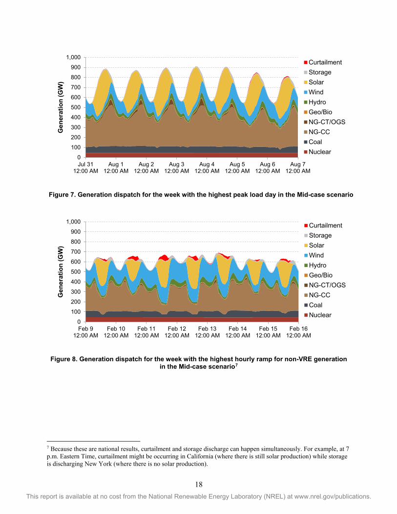
More-detailed system operation for the Mid-case in 2050 is shown in Figure 8 and Figure 9, which were generated using an hourly production cost model. Figure 8 shows the week with the highest national peak demand, which reaches 900 GW. PV generation is abundant during the daytime, while wind has higher generation overnight. The bulk of the variability is met by NG-CC units, but as the PV output declines, NG-CT, storage, and any flexible hydropower units also respond to the changing generation. Coal and nuclear provide a near-constant stream of power throughout the week. Figure 9, on the other hand, shows the week with the largest hourly ramp by the non-VRE generation. Load is much steadier between day and night, but VRE generation can vary considerably. NG-CC units continue to provide the bulk of the flexibility, but NG-CTs, hydropower, coal, storage and curtailed VRE (during both daytime and nighttime hours) also provide nontrivial amounts of flexibility.
0%
10%
20%
30%
40%
50%
60%
70%
80%
90%
100%
2018 2023 2028 2033 2038 2043 2048
Flee
t-wid
e C
apac
ity F
acto
r
Nuclear
Coal
Solar
NG-CCOther RE
Wind
18 This report is available at no cost from the National Renewable Energy Laboratory (NREL) at www.nrel.gov/publications.
Figure 7. Generation dispatch for the week with the highest peak load day in the Mid-case scenario
Figure 8. Generation dispatch for the week with the highest hourly ramp for non-VRE generation
in the Mid-case scenario7
7 Because these are national results, curtailment and storage discharge can happen simultaneously. For example, at 7 p.m. Eastern Time, curtailment might be occurring in California (where there is still solar production) while storage is discharging New York (where there is no solar production).
0
100
200
300
400
500
600
700
800
900
1,000
Jul 3112:00 AM
Aug 112:00 AM
Aug 212:00 AM
Aug 312:00 AM
Aug 412:00 AM
Aug 512:00 AM
Aug 612:00 AM
Aug 712:00 AM
Gen
erat
ion
(GW
)CurtailmentStorageSolarWindHydroGeo/BioNG-CT/OGSNG-CCCoalNuclear
0
100
200
300
400
500
600
700
800
900
1,000
Feb 912:00 AM
Feb 1012:00 AM
Feb 1112:00 AM
Feb 1212:00 AM
Feb 1312:00 AM
Feb 1412:00 AM
Feb 1512:00 AM
Feb 1612:00 AM
Gen
erat
ion
(GW
)
CurtailmentStorageSolarWindHydroGeo/BioNG-CT/OGSNG-CCCoalNuclear

19 This report is available at no cost from the National Renewable Energy Laboratory (NREL) at www.nrel.gov/publications.
Table 3 summarizes the relevant metrics for VRE for the Mid-case scenario in 2050 using the hourly production cost model results. The maximum hourly generation occurred in the summer afternoon, but the maximum hourly VRE penetration (as a share of total generation) occurred in the spring afternoon during a period of relatively lower load. The range in absolute and relative hourly VRE levels varies by an order of magnitude over the course of a year.
Table 3. Summary of National VRE Metrics from the Mid-case Scenario for 2050 Using the Hourly Production Cost Simulation
Metric Level Occurrence
Maximum hourly VRE penetration 77.2% Mid-afternoon in April
Minimum hourly VRE penetration 8.2% Early morning in September
Maximum VRE generation 549,500 MW Mid-afternoon in June
Minimum VRE generation 41,400 MW Early morning in September
Maximum VRE curtailment 147,700 MW Mid-afternoon in March
Key Insights • Wind and solar capacity grow significantly across nearly all scenarios. Natural gas
prices and renewable energy costs are significant drivers of the level of growth, and combinations of those two factors can lead to very high levels of growth, or very limited growth.
• Increasing shares of VRE lead to increased needs for seasonal and hourly flexibility. The variation across seasons, time of day, and hours observed in these scenarios from VRE require some level of flexibility from the rest of the generation fleet in order to ensure supply and demand are always in balance. Wind and PV can also complement one another in daily and seasonal trends.
• Future scenarios show higher levels of overall flexibility. Lower NG-CC capacity factors, increased transmission builds, and increased storage deployment lead to more overall flexibility across the system. Coal and nuclear operate with high capacity factors even with these higher levels of VRE.

20 This report is available at no cost from the National Renewable Energy Laboratory (NREL) at www.nrel.gov/publications.
3.3 The Potential for Renewable Energy Technologies Other than PV and Land-based Wind
Recent Trends
Figure 9. Annual U.S. capacity additions since 2010 of renewable technologies that are neither land-based wind nor solar PV. Note that this does not consider retired capacity due to replacement of
existing generators; therefore, net capacity additions, specifically those from hydroelectric, will be smaller due to refurbishment and upgrades of generators at existing facilities.
Hydropower and Pumped-Storage Hydropower With over 1,800 MW of additions since 2010, hydropower has the third largest amount of new renewable capacity behind land-based wind and solar PV. Though hydropower has historically involved creation of new dams and significant alterations of waterways, more recent development has involved improving and repowering existing infrastructure, both reducing costs and limiting environmental impacts. These projects are referred to as refurbishments and upgrades (R&U), which upgrade existing generators with new, more-efficient equipment, and non-powered dams (NPD), which add generating equipment to existing impoundments and reservoirs that do not currently have generating equipment.
0
200
400
600
800
1,000
1,200
2010 2011 2012 2013 2014 2015 2016 2017
Cap
acity
Add
ition
s (M
W)
IvanpahSolana
Genesis
Mojave
CrescentDunes
Hydro-electric
Geothermal
Offshore Wind(Block Island)
CSP
Pumped Storage

21 This report is available at no cost from the National Renewable Energy Laboratory (NREL) at www.nrel.gov/publications.
Figure 10. Distribution of gross hydropower capacity additions since 2010 by nameplate capacity
of each installation for cumulative capacity (left) and number of installations (right). Data are from EIA Form 860m for April 2018 (EIA 2018b).
The left side of Figure 11 illustrates how even though a few large-scale hydropower capacity additions dominate the total number of megawatts, none of them involves construction of new dams. The Wanapum and Cheoah are R&U projects that involve upgrading existing facilities with newer higher efficiency turbines and equipment (HydroWorld 2010; Grant PUD 2018). The Holtwood addition is an expansion of an existing facility with additional capacity (HydroWorld 2013), and the Meldahl employs run-of-river technology that takes advantage of an existing non-powered dam (AMP 2018).
Small hydropower facilities have comprised a significant share of capacity additions since 2010. As seen in Figure 11, 49 hydroelectric facilities of 10 MW or less have comprised nearly 200 MW of capacity additions. These generators provide benefits because they can take advantage of existing infrastructure and can have reduced environmental impacts, as they typically do not require construction of new impoundments. As an example, the Shavano Falls project in western Colorado uses five small generators, each having between 2 MW and 5 MW of capacity, that are located on existing irrigation channels and conduits (Segerstrom 2018).
Although only one new PSH facility has been commissioned recently (commissioned in 2012), it also takes advantage of existing infrastructure. The 42-MW Lake Hodges facility in California connects two existing reservoirs, providing both with PSH capabilities and expanding water access for San Diego County (San Diego County Water Authority 2018).
Near-term proposed projects continue this trend; at the end of 2017, there were 1,712 MW of proposed projects across 214 individual facilities, most of which were powering non-powered dams and adding capacity to existing conduits. Pumped-storage hydropower has 48 proposed projects, mostly in the early planning stage, however most of the projects use “closed-loop” systems that do not require them to be located on existing waterways (Uría-Martínez, Johnson, and O’Connor 2018).
0
200
400
600
800
1,000
1,200
1,400
0 - 10 10 - 100 100+
Tota
l Cap
acity
(MW
)
Nameplate Capacity (MW)
0
10
20
30
40
50
60
0 - 10 10 - 100 100+
Num
ber o
f Hyd
ro F
acili
ties
Nameplate Capacity (MW)
Wanapum R&U
Meldahl NPD
Holtwood Expansion
Cheoah R&U

22 This report is available at no cost from the National Renewable Energy Laboratory (NREL) at www.nrel.gov/publications.
Concentrating Solar Power (CSP) The next largest source of capacity additions is concentrating solar power (CSP), all of which came online between 2013 and 2015 (Figure 10) and of which is all located in the Southwest. These additions, totaling over 1,200 MW, are comprised of five separate projects across a range of different technologies and configurations:
• Solana: This 250-MW trough technology including six hours of molten salt storage capacity, came online in Arizona in 2013.
• Genesis and Mojave: Both projects, in California, are trough technology without storage, each is 250 MW, and they both came online in 2014.
• Ivanpah: The first large-scale “solar power tower” project in the United States with 377 MW of capacity also came online in 2014 in California.
• Crescent Dunes: The second solar power tower project, 110 MW with 10 hours of built-in thermal storage, became commercially operational in Nevada in 2015.
After this flurry of activity however, no other utility-scale CSP projects have been built in the United States, nor are any projects currently moving toward construction (Bolinger, Seel, and LaCommare 2017); this is likely due to the relative competitiveness of CSP projects with solar PV technologies. Figure 12 highlights how the power purchase agreement (PPA) prices for these five facilities were competitive with other utility-scale PV PPA prices when they were signed between 2009 and 2011. However, PV prices have since declined substantially while the absence of new CSP projects seems to indicate that CSP prices have not seen the same reduction.
Figure 11. Levelized power purchase agreement (PPA) prices for recent CSP projects relative to PV prices in comparable regions (Bolinger, Seel, and LaCommare 2017)

23 This report is available at no cost from the National Renewable Energy Laboratory (NREL) at www.nrel.gov/publications.
Geothermal Since 2010, geothermal capacity additions were fairly consistent, with additions occurring in every year except 2016. Overall, there were 17 geothermal capacity additions since 2010, with most of them occurring in Nevada and the rest coming online in other western states and Hawaii (EIA 2018b). The most recent development was the 24-MW Tungsten Mountain project in Nevada (Ormat Technologies 2017).
Overall, the development process for a geothermal facility is more similar to that of oil and gas projects. Resources are identified and developed through exploration, assessment, and ultimately drilling to access subsurface resources. As a result, geothermal facilities can be costly to develop. However, as with hydropower development, costs can be reduced by utilizing existing infrastructure. For example, the Wabuska generator in Nevada has been operating since the 1980s, but it was expanded in 2002 and again in 2011 with additional generators (Open Mountain Energy 2017). In such examples, costs are reduced, as the resource quality of the site is better characterized than greenfield sites (i.e., reducing risk) and the required grid connection already exists.
No geothermal projects are currently under active construction, but as of 2016, 80 potential projects were in various early stages of exploration and development, with approximately 500 MW of potential capacity awaiting financing and purchasing agreements. The U.S. Energy Information Administration indicates that as of April 2018 four projects totaling 163 MW were in the later stages of development and awaiting regulatory approval (EIA 2018b; Matek 2016).
Though enhanced geothermal systems (EGS) technologies have not yet reached commercial development, three multi-year demonstration projects were underway in 2016. In addition, The U.S. Department of Energy (DOE) is evaluating sites for the Frontier Observatory for Research in Geothermal Energy (FORGE), a facility for testing targeted EGS research and development (Beiter, Vincent, and Ma 2018).
Offshore Wind (OSW) Though offshore wind (OSW) has grown globally and had over 17,000 MW of capacity globally by the end of 2017, the United States accounts for only a small fraction of that capacity. The first and currently only OSW facility in operation in the United States is the 30-MW Block Island wind farm off the coast of Rhode Island, which began operating in late 2016.
Global auctions for OSW development in Europe indicate that costs are declining for this technology as seen in Figure 13. Even though not all possible differences between projects are accounted for, the decline of prices from ~$200/MWh for projects coming online in 2017–2019 to ~$65/MWh for facilities with planned operational dates of 2024–2025 is significant (Musial et al. 2017). Though it is not yet certain that these cost declines will translate into similar reductions for U.S. projects, the recent announcement of a PPA for 800 MW of OSW in Massachusetts with prices as low as $65/MWh indicates it could be possible (Bade 2018).

24 This report is available at no cost from the National Renewable Energy Laboratory (NREL) at www.nrel.gov/publications.
Figure 12. Adjusted price strike from recent European OSW auctions. The “strike price” is the
winning auction price. Figure from Musial et al. (2017).*Grid and development costs added; **Grid costs added and contract length adjusted; ***Development costs added
Though no additional OSW projects are currently under construction in the United States, there is a significant pipeline of potential projects, with over 24,000 MW of capacity identified in various early stages of development (Musial et al. 2017). Though not all of this pipeline may ultimately be brought to commercial operations, a substantial amount of recent activities indicate future domestic growth in OSW is likely, including recent additional supporting state-level policies in Maryland, Massachusetts, and New York, and increased leasing activities specifically for OSW development from the U.S. Bureau of Ocean Energy Management (Musial et al. 2017).
Outlook Hydropower, Geothermal, and OSW—Competition with VRE and Natural Gas Conventional hydropower and geothermal have similar technology characteristics, which is perhaps why they might have similar results across the scenarios. Both are typically geographically constrained technologies with site-specific costs and generation profiles, and both can offer dispatchable renewable generation with the ability to provide some flexibility and ancillary services.
As observed in the scenario results in Figure 14, both technologies see a limited range of capacity deployment by 2050: ~80–83 GW for hydropower (relative to a starting point of ~76 GW) and ~3–8 GW for geothermal. For both, more-aggressive cost reduction assumptions are

25 This report is available at no cost from the National Renewable Energy Laboratory (NREL) at www.nrel.gov/publications.
insufficient to drive further deployment over the Mid-case beyond a few hundred megawatts.8 Both technologies appear to be in competition with other renewable technologies, namely wind and solar PV, as they both see enhanced deployment under the High RE Cost scenario.9 Both see the largest deployment under the High NG + High RE Cost scenario, which also highlighting the impact of relatively low-cost natural gas. Supporting this point, both technologies see reduced deployment over the Mid-case under Low NG + Low RE costs.
Figure 13. Hydropower capacity (left) and geothermal capacity (right) across the scenarios. Note differences in scale.
Specifically, for hydropower, early growth of 3–4 GW is driven by the PTC and the availability of low-cost upgrades for existing facilities.10 However, across the scenarios by 2050, there is a relatively narrow range of total hydropower capacity–80 to 83 GW—as seen in Figure 14, representing ~3-7 GW of new capacity. Hydropower cost reductions assumed to result from advances in hydropower R&D under the Low Hydro Cost case result in only a marginal increase in capacity relative to the Mid-case. Hydropower does see additional deployment under scenarios where the main competitors have higher costs. Both high natural gas costs and high renewable cost scenarios result in ~ 1 GW of additional deployment over the Mid-case, with the largest deployment scenario occurring in the combined High Natural Gas + High Renewable costs scenario.
8 The DOE Hydropower Vision Study (DOE 2016) and the DOE Geothermal Vision Study provide additional and broader perspectives on these two technologies. The Geothermal Vision Study is underway as of this writing. It includes updated cost and performance projections for geothermal technologies, but those projections were not available for this work; the results of the Geothermal Vision Study will therefore be different from those shown here, and they will include more-aggressive cost declines than those modeled in the Standard Scenarios. 9 The High RE Cost scenario has high costs for all renewable energy technologies. However, hydropower and geothermal have relatively smaller cost reductions in the Mid-case than wind and PV, so the change from Mid-case technology costs to high-case costs makes hydropower and geothermal more cost competitive relative to wind and PV. 10 Although ReEDS builds this capacity in the very near term, it might not be feasible for this capacity to be built so quickly even if it is cost-effective. For example, permitting timelines, water usage requirements, or other considerations might lengthen the timeline to perform these upgrades.
Mid-case
High RE Cost
Reduced RE
Resource
Low NG + Low RE
High NG + High RE
Low Hydro
75
76
77
78
79
80
81
82
83
84
85
2020 2030 2040 2050
Hyd
ropo
wer
Cap
acity
(GW
)
Mid-case
High RE Cost
Low Demand
Low NG + Low RE
High NG + High RE
Low Geo
0
1
2
3
4
5
6
7
8
9
2020 2030 2040 2050
Geo
ther
mal
Cap
acity
(GW
)

26 This report is available at no cost from the National Renewable Energy Laboratory (NREL) at www.nrel.gov/publications.
Similarly, for geothermal, low costs for this technology alone result in less than 1 GW of additional capacity over the Mid-case. The highest deployment is seen with high natural gas and high VRE costs, while a slight decrease in capacity results when both natural gas and wind and solar PV costs stay low.
Figure 14. Off-shore wind capacity deployment across scenarios. The High NG + Low Offshore Costs scenario is the only scenario that results in additional deployment beyond the Mid-case scenario.
While OSW sees less deployment overall due to more challenging economics, the level of deployment is sensitive to the same factors as geothermal and hydropower: natural gas prices and other renewable cost. OSW is expected to grow over the next decade or so as seen in Figure 15, driven in large part by the state-level policies and mandates, with up to 6 GW by 2030. However, the combination of competitive natural gas and land-based wind and solar PV costs challenges even lower-cost OSW projects. Unlike geothermal and hydropower technologies, there is no existing offshore infrastructure that could be leveraged to result in cost-savings. In general, each OSW project will need to build support structures and underwater cables to connect to the mainland. Only in the High NG and Low OSW Costs scenario is additional OSW capacity observed beyond the Mid-case in the 2040s.
There are a few additional factors not explicitly considered in the modeling framework to consider when interpreting these results. First, the natural gas infrastructure is not modeled in detail; new natural gas facilities are assumed to be able to connect to a natural gas pipeline or other source. If constraints on building new natural gas pipeline capacity arise in certain regions, alternative generation would be required. Secondly, the non-economic barriers to interstate transmission builds may be higher than is captured in the model. This would reduce the ability to access the lowest-cost wind and solar resources. Finally, several state and local policies support either local renewable development or 100% renewables; though not all are explicitly in the model, they indicate potential preference of local communities to renewable generation sourced near population centers. If these situations arose, they would contribute to scenarios that might support additional OSW development.
Mid-case
High NG + Low
Offshore
0
2
4
6
8
10
12
2020 2030 2040 2050
Offs
hore
Win
d C
apac
ity (G
W)

27 This report is available at no cost from the National Renewable Energy Laboratory (NREL) at www.nrel.gov/publications.
In addition, these technologies’ capacity deployment depends strongly on how refined the lower end of the supply curve is implemented in ReEDS. As indicated above, much of the recent new capacity of hydropower and geothermal is in lower-cost locations that utilize existing infrastructure such as expanding existing facilities. These opportunities are very site-specific and challenging to identify, quantify, and aggregate up to the level needed in ReEDS, and the current implementation shows only one potential set of outcomes.
Figure 15. Geothermal, hydropower, and OSW generation in 2050 relative to the Mid-case, across several scenarios. Note that some combination scenarios (e.g., High NG and Low RE) appear twice.
Results from the full set of scenarios indicate that onshore wind and solar technologies represent the main competition for future deployment of hydropower, geothermal, and OSW (see Figure 16). In other words, the success of the three technologies will depend on how competitive solar and onshore wind might be and is less sensitive to natural gas prices. Overall, competition from other fuels, the overall lack of capacity needs, and lack of demand growth, lead to minimal demand for capacity from these three technologies.
-40
-30
-20
-10
0
10
20
30
40
Hig
h N
G P
rice
Hig
h N
G +
Hig
h R
EH
igh
NG
+ L
ow G
eoH
igh
NG
+ L
ow H
ydro
Hig
h N
G +
Low
Offs
hore
Low
NG
Pric
eLo
w N
G +
Hig
h R
ELo
w N
G +
Low
Geo
Low
NG
+ L
ow H
ydro
Low
NG
+ L
ow O
ffsho
reLo
w N
G +
Low
RE
Low
NG
+ L
ow C
SP
Hig
h R
E C
ost
Hig
h N
G +
Hig
h R
ELo
w N
G +
Hig
h R
E
Low
RE
Cos
tLo
w P
V C
ost
Low
Win
d C
ost
Low
CSP
Low
NG
+ L
ow C
SPLo
w N
G +
Low
RE
2050
Geo
ther
mal
, Hyd
ropo
wer
, and
O
SW G
ener
atio
n R
elat
ive
to M
id-
Cas
e(TW
h)
Scenarios
OSW
Geothermal
Hydropower
High NG Price Low NG Price High RE Cost Low RE

28 This report is available at no cost from the National Renewable Energy Laboratory (NREL) at www.nrel.gov/publications.
Concentrating Solar Power and Pumped-Storage Hydropower—Potential for Large Growth
Figure 16. Deployment of CSP and PSH capacity across the scenarios. Note differences in scale.
Unlike the three technologies just examined, CSP and PSH generally see little to no additional deployment across the scenarios except for a few key scenarios where capacity grows dramatically. Expanded CSP deployment is contingent on more-aggressive CSP cost reductions. Deployment of CSP across the scenarios is fairly consistent with little to no deployment beyond existing facilities through the mid-2030s as seen in Figure 17. However, if CSP achieves more-aggressive cost reductions, deployment of over 40 GW is observed in the 2040s. Even with sustained low natural gas prices, low CSP costs would still enable nearly 12 GW of additional deployment by 2050. Under a combination of high natural gas and low CSP costs, the model shows over 160 GW of CSP capacity by 2050.
This relationship with natural gas prices arises in part because the greatest cost reductions in the low-cost CSP scenario are in the CSP field and storage, facilitating CSP configuration with high solar multiples and large amounts (>12 hours) of storage. Therefore, low-cost CSP with storage is a flexible generation resource that can be dispatched with the same level of flexibility as natural gas generators. In addition, although the highest quality CSP resource is located in the Southwest, specific CSP locations are not as geographically constrained as site-specific hydropower and geothermal capacity.
Similarly, a few scenarios lead to relatively large increases in PSH, although they are more contingent on VRE penetration than they are on low PSH costs. PSH capacity across the scenarios is also generally fairly narrow within a range of 0–4 GW over 2016 levels with 1.7 GW of additional growth in the Mid-case, generally occurring in the 2040s. However, unlike with conventional hydropower, a few scenarios result in additional deployment of 15–35 GW, with deployment occurring between 2030 and 2050. Similar to conventional hydropower, the drivers for this additional deployment arise in scenarios that have high natural gas prices. However, unlike conventional hydropower, PSH also increases in scenarios that have high penetrations of wind and solar such as the Low RE Cost scenario, as seen in Figure 18. This highlights the role
Mid-case
High NG + Low RE
High NG + Low CSP
Low CSP
Low NG + Low CSP
0
20
40
60
80
100
120
140
160
180
2020 2030 2040 2050
CSP
Dep
loym
ent (
GW
)
Mid-case
Low RE Cost
High NG Price
High NG + Low RE
High NG + High RE
High NG + Low Hydro
Low Hydro
0
10
20
30
40
50
60
2020 2030 2040 2050PS
H C
apac
ity (G
W)

29 This report is available at no cost from the National Renewable Energy Laboratory (NREL) at www.nrel.gov/publications.
of PSH in providing capacity and long-term storage of renewables under higher penetrations, or when natural gas is uneconomic.
Figure 17. PSH capacity in 2050 versus the 2050 VRE penetration
Key Insights • Geothermal, hydropower, and OSW see a narrow range of deployment outcomes
across the scenarios, which is highly dependent on competition from other low-cost renewables and natural gas. Assumed lower costs for these resources alone are generally insufficient to drive significant new deployment. The site-specific cost dependency of these resources may limit broader deployment but might provide low-cost opportunities for utilizing existing infrastructure.
• Broader CSP deployment hinges on CSP achieving more-aggressive cost reductions than are assumed in the Mid-case. In conjunction with this, competition with natural gas is more important than is competition from other renewables.
• Higher PSH capacity is driven by synergies with VRE deployment. Unlike the other technologies in this section, PSH is not in competition with VRE, but it can provide value by reducing curtailment and providing capacity under high VRE scenarios.
Mid-case
Low RE Cost
Low PV Cost
Low Wind Cost
High NG Price
High NG + Low RE
High NG + Low Hydro
0
10
20
30
40
50
60
70
0% 10% 20% 30% 40% 50% 60% 70% 80%
PSH
Dep
loym
ent (
GW
)
VRE Penetration
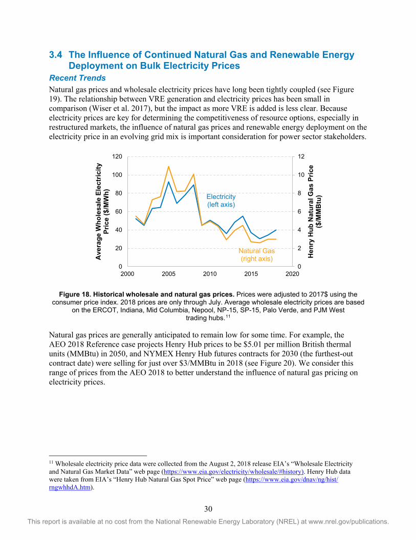
30 This report is available at no cost from the National Renewable Energy Laboratory (NREL) at www.nrel.gov/publications.
3.4 The Influence of Continued Natural Gas and Renewable Energy Deployment on Bulk Electricity Prices
Recent Trends Natural gas prices and wholesale electricity prices have long been tightly coupled (see Figure 19). The relationship between VRE generation and electricity prices has been small in comparison (Wiser et al. 2017), but the impact as more VRE is added is less clear. Because electricity prices are key for determining the competitiveness of resource options, especially in restructured markets, the influence of natural gas prices and renewable energy deployment on the electricity price in an evolving grid mix is important consideration for power sector stakeholders.
Figure 18. Historical wholesale and natural gas prices. Prices were adjusted to 2017$ using the consumer price index. 2018 prices are only through July. Average wholesale electricity prices are based
on the ERCOT, Indiana, Mid Columbia, Nepool, NP-15, SP-15, Palo Verde, and PJM West trading hubs.11
Natural gas prices are generally anticipated to remain low for some time. For example, the AEO 2018 Reference case projects Henry Hub prices to be $5.01 per million British thermal units (MMBtu) in 2050, and NYMEX Henry Hub futures contracts for 2030 (the furthest-out contract date) were selling for just over $3/MMBtu in 2018 (see Figure 20). We consider this range of prices from the AEO 2018 to better understand the influence of natural gas pricing on electricity prices.
11 Wholesale electricity price data were collected from the August 2, 2018 release EIA’s “Wholesale Electricity and Natural Gas Market Data” web page (https://www.eia.gov/electricity/wholesale/#history). Henry Hub data were taken from EIA’s “Henry Hub Natural Gas Spot Price” web page (https://www.eia.gov/dnav/ng/hist/ rngwhhdA.htm).
0
2
4
6
8
10
12
0
20
40
60
80
100
120
2000 2005 2010 2015 2020
Hen
ry H
ub N
atur
al G
as P
rice
($/M
MB
tu)
Ave
rage
Who
lesa
le E
lect
ricity
Pr
ice
($/M
Wh) Electricity
(left axis)
Natural Gas (right axis)
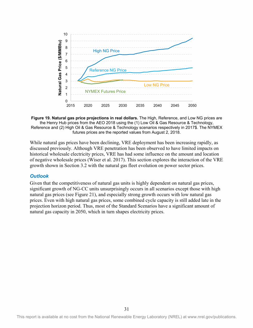
31 This report is available at no cost from the National Renewable Energy Laboratory (NREL) at www.nrel.gov/publications.
Figure 19. Natural gas price projections in real dollars. The High, Reference, and Low NG prices are the Henry Hub prices from the AEO 2018 using the (1) Low Oil & Gas Resource & Technology,
Reference and (2) High Oil & Gas Resource & Technology scenarios respectively in 2017$. The NYMEX futures prices are the reported values from August 2, 2018.
While natural gas prices have been declining, VRE deployment has been increasing rapidly, as discussed previously. Although VRE penetration has been observed to have limited impacts on historical wholesale electricity prices, VRE has had some influence on the amount and location of negative wholesale prices (Wiser et al. 2017). This section explores the interaction of the VRE growth shown in Section 3.2 with the natural gas fleet evolution on power sector prices.
Outlook Given that the competitiveness of natural gas units is highly dependent on natural gas prices, significant growth of NG-CC units unsurprisingly occurs in all scenarios except those with high natural gas prices (see Figure 21), and especially strong growth occurs with low natural gas prices. Even with high natural gas prices, some combined cycle capacity is still added late in the projection horizon period. Thus, most of the Standard Scenarios have a significant amount of natural gas capacity in 2050, which in turn shapes electricity prices.
0
1
2
3
4
5
6
7
8
9
10
2015 2020 2025 2030 2035 2040 2045 2050
Nat
ural
Gas
Pric
e ($
/MM
Btu
)
High NG Price
Reference NG Price
Low NG PriceNYMEX Futures Price

32 This report is available at no cost from the National Renewable Energy Laboratory (NREL) at www.nrel.gov/publications.
Figure 20. Natural gas combined cycle capacity in the non-policy scenarios. Core natural gas price and renewable energy cost sensitivity scenarios are also highlighted.
Figure 22 shows the evolution of marginal energy prices over time. The marginal energy price is a modeled electricity price—specifically the annual load-weighted average of the shadow price of the load-balancing constraint.12 These prices are, in concept, similar to locational marginal prices in current electricity markets, but they do not capture all hourly fluctuations driven by events such as extreme weather events, plant or transmission outages, or behavior from the competitive bidding process in real markets. Unsurprisingly, scenarios with high natural gas price assumptions tend to have the highest marginal energy prices while those with low natural gas price assumptions have the lowest. However, the interaction with the assumed renewable energy costs becomes quite important. For example, in the High NG Price + Low RE Cost scenario, the lower renewable energy costs mitigate the impact on the marginal energy price from the higher natural gas prices. Similarly, in the Low NG Price + High RE Cost, the higher renewable energy costs lead to marginal energy prices equivalent to the Mid-case despite the low natural gas price assumption. Some of this effect in prices is do a shifting of the merit order. An increase of the zero marginal cost generators pushes the supply curve to the right, potentially resulting in a more efficient or lower cost unit setting the marginal price.
12 This modeled electricity price is the marginal cost in the model of providing one more unit of energy. It does not include other electricity cost components such as ancillary service provision or firm capacity requirements.
Mid-case
Low RE Cost
High RE Cost
Low NG Price
High NG Price
High NG + Low RE
Low NG + High RE
0
100
200
300
400
500
600
700
800
2020 2030 2040 2050
NG
-CC
Cap
acity
(GW
)

33 This report is available at no cost from the National Renewable Energy Laboratory (NREL) at www.nrel.gov/publications.
Figure 21. National average marginal electricity prices for the non-policy scenarios. The combination scenarios with high and low natural gas prices and high and low renewable energy
costs are highlighted more than once.
This interaction between natural gas prices and renewable energy costs is further explained by Figure 23. The relationship between the marginal energy price and natural gas prices is linear, with higher gas prices leading to higher marginal energy prices (see also Figure 24, which shows the same relationship but with higher spatial and temporal resolution). The low and high renewable energy cost scenarios generally follow this linear relationship. However, one can see that the low renewable energy cost scenarios generally have lower natural gas prices and the high renewable energy cost scenarios generally have higher natural gas prices. Section 3.2 showed that renewable energy penetration is higher in scenarios with lower cost, and because of the higher penetration, less natural gas is used to meet system needs. The lower natural gas demand leads to lower natural gas prices, but because natural gas generators are still largely on the margin, they are still setting the marginal price. The opposite effect is true of the high renewable energy cost scenarios; specifically, high renewable energy costs lead to a greater demand for natural gas, which in turn leads to higher prices. Thus, one of renewable energy’s effects on the annual average marginal energy price is its impacts on the demand for natural gas. In turn that implies that how one treats the elasticity of natural gas can have a significant impact on the absolute level of electricity prices anticipated.
0
10
20
30
40
50
60
70
2020 2030 2040 2050
Mar
gina
l Ene
rgy
Pric
e ($
/MW
h) High NG Price Scenarios
Low NG Price Scenarios
2020 2030 2040 2050
Low RE Cost Scenarios
2020 2030 2040 2050
High RE Cost Scenarios

34 This report is available at no cost from the National Renewable Energy Laboratory (NREL) at www.nrel.gov/publications.
Figure 22. National average natural gas price in 2050 versus the national average marginal energy price in 2050 for the non-policy scenarios.
Figure 23. Marginal energy price versus natural gas price for each ReEDS balancing area in each year for the Mid-case, Low NG Price, and High NG Price scenarios
The interaction of generally lower electricity prices (associated high VRE penetration) with the generally reduced utilization of some dispatchable plants in order to provide flexibility (e.g., Figure 7 shows the NG-CC capacity factor declines over time) leads to a system where the value of dispatchable capacity tends to increase over time. For example, Figure 25 shows that for a new NG-CC unit in the Mid-case scenario, the fraction of fixed costs (annualized capital costs plus fixed operations and maintenance costs) recovered by the capacity value increases over time. By the 2040s, over 80% of the fixed costs of NG-CC units are recovered in the model through capacity.
0
10
20
30
40
50
60
70
0 2 4 6 8 10 12
Mar
gina
l Ene
rgy
Pric
e in
205
0 ($
/MW
h)
Natural Gas Price in 2050 ($/MMBtu)
Low RE CostMid RE CostHigh RE Cost
0
10
20
30
40
50
60
70
0 2 4 6 8 10Mar
gina
l Ene
rgy
Pric
e ($
/MW
h)
Natural Gas Price ($/MMBtu)
High NG Price
Low NG Price Mid-case

35 This report is available at no cost from the National Renewable Energy Laboratory (NREL) at www.nrel.gov/publications.
Figure 24. Relative fraction of the fixed costs that are recovered from capacity versus energy and ancillary services for a new NG-CC plant in the Mid-case.
Another effect of renewable energy on the marginal energy prices is seen in Figure 26, which shows the marginal energy price in the summer for the Mid-case and Low RE Cost scenarios. The average marginal energy price at the start of the evaluation period is highest in the afternoon and lowest overnight. However, as VRE resources grow, that relationship changes. In the Mid-case scenario, the evening becomes the most expensive time of day because of the increase in PV deployment, and the lowest-cost period shifts to mornings. The Low RE Cost scenarios considers the effects of even higher VRE deployment. In this scenario, the afternoon becomes the lowest-cost period, but as in the Mid-case, the evening is the most expensive period for most of the model horizon.
Figure 25. National average marginal energy price by time of day for the summer in the Mid-case (left) and Low RE Cost (right) scenarios
0%10%20%30%40%50%60%70%80%90%
100%
2020
2022
2024
2026
2028
2030
2032
2034
2036
2038
2040
2042
2044
2046
2048
2050Fr
actio
n of
Fix
ed C
osts
Rec
over
ed
by N
G-C
C U
nits
Capacity Value Energy & Ancillary Service Value
0
5
10
15
20
25
30
35
40
45
50
2018 2028 2038 2048
Mar
gina
l Ene
rgy
Pric
e ($
/MW
h)
2018 2028 2038 2048
NightMorningAfternoonEvening
Mid-case Low RE Cost

36 This report is available at no cost from the National Renewable Energy Laboratory (NREL) at www.nrel.gov/publications.
Because the Mid-case was also run in an hourly production cost model, additional granularity is available in modeled electricity prices for that scenario. Figure 27 shows the number of hours in every ReEDS balancing area where the marginal energy price is at or below $1/MWh. All balancing areas have prices at less than $1/MWh for at least 100 hours of the year, and more than half see fewer than 1,000 of these low-price hours. A few have more than 4,000 hours below this price threshold. These regions are typically remote (and low-load) regions near the edge of an interconnection with much high-quality wind resource. The hours with less than $1/MWh marginal energy price comprise 10% of the total annual load and represent 14% of all hours in the year. For reference, in 2016 less than 2% of hours in real-time markets had negative prices, and outside of California there were virtually no negative price hours in the day-ahead markets (California had negative prices in ~0.5% of hours in the day-ahead market) (Wiser et al. 2017).
Figure 26. Number of hours where the marginal energy prices are at or below $1/MWh in each ReEDS region in 2050 for the Mid-case. The 134 ReEDS regions have been sorted from those with the
highest number of hours at or below $1/MWh to those with the least.
Key Insights • Natural gas combined cycle capacity grows considerably across nearly all scenarios.
Growing demand, retirements, and increased flexibility needs lead to higher levels of NG-CC capacity in all scenarios. NG-CC builds are particularly sensitive to natural gas prices and renewable energy costs.
• Marginal electricity prices continue to be impacted primarily by natural gas prices. The modeled scenarios showed a linear relationship between natural gas prices and marginal electricity prices across most scenarios. Scenarios with higher or lower renewable energy deployment tended to impact the electricity prices by changing the demand for natural gas, which in turn impacts the price.
• Increased VRE levels lead to changes in time-of-day price patterns and to a significant number of low-price hours. Currently, afternoon periods typically have the highest prices, but the most expensive period tends to shift to the evening, with the daytime hours becoming lower-cost time periods in scenarios with extensive PV
0
1,000
2,000
3,000
4,000
5,000
6,000
0 20 40 60 80 100 120 140
Num
ber o
f Hou
rs w
ith P
rice
Bel
ow $
1/M
Wh
Number of ReEDS Balancing Areas

37 This report is available at no cost from the National Renewable Energy Laboratory (NREL) at www.nrel.gov/publications.
deployment. The number of low-price (less than $1/MWh) hours is significant in 2050, with all regions experiencing at least hundreds of low-price hours in the Mid-case.
3.5 What Happens to Renewable Energy Deployment After the Tax
Credits Phase Out? Recent Trends Much of the recent growth in renewable energy in the electric power sector can be attributed to policy support and declining capital costs that have made renewable energy technologies, particularly wind and PV, cost competitive with other traditional generating resources (Mundaca and Luth Richter 2015; Jensen and Dowlatabadi 2017; Stokes and Breetz 2018). Specifically, the federal production tax credit (PTC) and the federal investment tax credit (ITC) have contributed significantly to the growth of wind and PV respectively. Recently, these tax credits were extended but with a gradual step-down in value over multiple years with the intention of phasing them out.
The PTC offers a 10-year credit of 2.3 cents per kilowatt-hour for wind and other qualifying technologies. It was originally enacted in 1992 and it was extended 10 times between 1999 and 2015, and over that time, it lapsed and was extended retroactively five times (Sherlock 2015). The policy uncertainty during this period created a volatile market with a boom-and-bust cycle that followed the lapses and extensions of the tax credit as shown in Figure 28 (Wiser and Bolinger 2017). The ITC offers a payment of 30% of capital expenditures for the construction of a PV system or other qualifying technology. It was originally enacted in 2005, later extended through 2008, and then extended for eight more years as part of the Emergency Economic Stabilization Act of 2008 (Stokes and Breetz 2018). PV has experienced fewer lapses, but the same boom-and-bust response can be seen in the record deployment in 2016 following the extension of the PTC and ITC in December 2015 (see Figure 28).
Figure 27. Annual wind capacity additions with PTC history and annual PV capacity additions with
ITC history. PTC figure adapted from Mai et al. (2016).
Outlook Following the expiration of the PTC, most scenarios show little to no growth in wind capacity for several years (see Figure 29). Some scenarios show wind capacity stagnant or even declining for many years. Drivers of this slow wind growth are as expected, with low natural gas prices,

38 This report is available at no cost from the National Renewable Energy Laboratory (NREL) at www.nrel.gov/publications.
high wind costs, and low demand, which all push demand for new wind downward. Conversely, scenarios with high natural gas prices and low wind cost projections have the largest upside potential for wind deployment. These high wind growth scenarios still experience a slow-down in wind deployments following the expiration of the PTC, but it is limited both in duration and magnitude. The PTC & ITC Extension scenario (which extends both tax credits at their full value through 2030 after stepping down as scheduled) results in rapid expansion of the wind fleet while the PTC is in effect. However, after the PTC expires in 2030, total deployment already exceeds the 2050 deployment in the Mid-case, and no new net capacity is added through 2050.13
Figure 28. Wind generation across the non-policy scenarios and including the PTC & ITC Extension scenario (in green). Several scenarios with wind generation exceeding the Mid-case are
highlighted.
In contrast to wind, PV continues to grow in all scenarios after the step-down of the ITC. As with wind, this growth is greatest in scenarios with high natural gas prices or low PV costs and is least with low natural gas prices or high PV costs. The PTC & ITC Extension scenario has a lesser impact on PV than wind does, partly because of the structure of the PTC versus the ITC. Because the PTC is constant in absolute terms ($23/MWh), its relative value grows as capital costs decline and/or as capacity factors improve. On the other hand, the ITC is constant in relative terms (30% of capital costs), but its absolute value declines as capital costs come down over time. This can be seen in Figure 30, which shows the LCOE of an average wind and PV resource with no tax credit, the phased-down tax credit, and the extended tax credit. In 2016, the PTC reduces the LCOE of wind by 29%, but in 2030, that value grows to 36%. For PV, the absolute value of the ITC decreases from $26/MWh in 2016 to $12/MWh in 2030. Additionally, the ITC for non-residential PV remains at 10% after the step-down, so the relative change of going from 30% to 10% (instead of 0%) somewhat reduces the impact on PV deployment.
13 Rebuilds still occur as older wind plants reach the end of their lives.
Mid-case
Low RE Cost
Low Wind Cost
High NG Price
PTC & ITC Extension
High NG + Low RE
0
500
1,000
1,500
2,000
2,500
2020 2030 2040 2050
Win
d G
ener
atio
n (T
Wh)

39 This report is available at no cost from the National Renewable Energy Laboratory (NREL) at www.nrel.gov/publications.
Figure 29. Total PV generation across the non-policy scenarios and including the PTC & ITC Extension scenario (in green). Several scenarios with PV generation exceeding the Mid-case are
highlighted. PV capacity includes both utility-scale and rooftop PV.
Figure 30. LCOE of wind (left) and PV (right) assuming average resource availability.
LCOE assumptions for average wind and PV resources (Techno-Resource Group 4 for wind and Kansas City for PV) from the 2018 Annual Technology Baseline (ATB) (NREL 2018). Total height shows real LCOE without any tax credits, sub-heights show LCOE with the current sunset timeline and with an
extension through 2030. Financing inputs were held constant across all years and tax credit settings, and a 20-year evaluation period was used.
Utility-scale PV in the PTC & ITC Extension scenario is 43 GW (20%) higher than it is in the Mid-case. Rooftop PV, on the other hand, is 20 GW (50%) higher in the PTC & ITC Extension scenario than it is in the Mid-case. The impact of the ITC extension or decline is felt more strongly in the residential sector, where the credit decreases from 30% to 0% than in the commercial and industrial sectors, where it declines to 10%.
Mid-case
Low RE Cost
Low PV Cost
High NG Price
PTC & ITC Extension
High NG + Low RE
0
200
400
600
800
1,000
1,200
1,400
1,600
1,800
2020 2030 2040 2050
PV G
ener
atio
n (T
Wh)

40 This report is available at no cost from the National Renewable Energy Laboratory (NREL) at www.nrel.gov/publications.
Though these scenarios show deployment trajectories after the step-down of the tax credits in an optimization model, they do not capture other effects of market actors. For example, corporate purchasers, new business models, and research and development activities in the wind industry might counteract the stagnant demand for wind observed in many of the scenarios. Conversely, supply chain bottlenecks or similar challenges might limit wind growth in some of the most aggressive wind and solar deployment scenarios.
The impacts resulting from the deployment levels shown above on CO2 emissions are shown in Figure 32. Natural gas prices have the largest impact on emissions in the near term, but over the long-term, emissions vary widely across the scenarios. Scenarios with higher levels of VRE deployment often, but not always lead to lower long-term CO2 emissions than the Mid-case. For example, the High NG Price scenario has more wind and PV deployment than the Mid-case scenario (see Figure 29 and Figure 30), but its emissions are higher than the Mid-case in most years. The PTC & ITC Extension scenario, with its higher near-term deployment of VRE, leads to lower CO2 emissions through the tax credit extension period, and then emissions slowly rise as new demand is met at least in part by new NG-CC generation.
Figure 31. CO2 emissions in the relevant scenarios. Core natural gas price and renewable energy cost
sensitivity scenarios, along with the tax credit extension scenario, are also highlighted.
Key Insights • Wind deployment slows after the expiration of the PTC. The magnitude and duration
of the slowdown varies widely across scenarios. In general, scenarios with higher natural gas prices and lower wind costs mitigate the slowdown.
• PV has steady deployment during and after the ITC step-down across the range of scenarios. Both rooftop PV and utility PV are impacted. The magnitude of PV deployment follows similar drivers as wind.
• Long-term CO2 emissions vary widely. Near-term emissions are most sensitive to natural gas prices. Long-term emissions are typically, but not always, lower in scenarios with high levels of renewable energy.
Mid-case
Low RE Cost
Low PV CostLow Wind Cost
High NG Price
PTC & ITC Extension
High NG + Low RE0
0.2
0.4
0.6
0.8
1
1.2
1.4
1.6
1.8
2
2020 2030 2040 2050
CO
2Em
issi
ons
(Bill
ion
Met
ric
Tons
)

41 This report is available at no cost from the National Renewable Energy Laboratory (NREL) at www.nrel.gov/publications.
4 Summary The Standard Scenarios provide a wide range of scenarios for the electricity power sector using complex electricity-sector models. The scenarios provide a benchmark for assessing trends and a data set to help advance thinking of how the power sector might evolve over time. We have highlighted several interesting story lines that we have observed from this suite of scenarios. Obviously, many others could also be considered. The purpose of this work is not to provide exhaustive analysis, but to provide a set of data and observations that can help advance critical thinking and decision-making in the power sector. Within NREL, we have found significant value in using the Standard Scenario to accelerate analysis and provide a baseline for related work. We share them with the hope that they can be of similar value to other power-sector stakeholders as they make decisions that will influence this constantly changing electricity sector.

42 This report is available at no cost from the National Renewable Energy Laboratory (NREL) at www.nrel.gov/publications.
5 References ABB. 2018. “ABB Velocity Suite.” http://new.abb.com/enterprise-software/energy-portfolio-management/market-intelligence-services/velocity-suite.
AMP. 2018. “Meldahl Hydro Project.” https://www.amppartners.org/generation/hydro/meldahl-hydro-project.
Bade, Gavin. 2018. “Massachusetts Utilities File US-Record Offshore Wind Contracts at $65/MWh | Utility Dive.” Utility Dive. August 2, 2018. https://www.utilitydive.com/news/massachusetts-utilities-file-us-record-offshore-wind-contracts-at-65mwh/529208/.
Beiter, Philipp C., Nina M. Vincent, and Ookie Ma. 2018. “2016 Renewable Energy Grid Integration Data Book.” NREL/BK-6A20-71151. Golden, CO: National Renewable Energy Laboratory. https://www.nrel.gov/docs/fy18osti/70231.pdf.
Bolinger, Mark, Joachim Seel, and Kristina LaCommare. 2017. “Utility-Scale Solar 2016: An Empirical Analysis of Project Cost, Performance, and Pricing Trends in the United States.” LBNL-2001055. Berkeley, CA: Lawrence Berkeley National Laboratory. https://emp.lbl.gov/sites/default/files/utility-scale_solar_2016_report.pdf.
CAISO (California Independent System Operator). 2018, July 24. Memorandum (from ISO Board of Governors To Steve Berberich, President and Chief Executive Officer). http://www.caiso.com/Documents/CEOReport-Jul2018.pdf.
Cole, Wesley J., Kelly P. Eurek, Nina M. Vincent, Trieu T. Mai, Gregory L. Brinkman, and Matthew Mowers. 2018. “Operating Reserves in Long-Term Planning Models.” NREL/PR-6A20-71148. Golden, CO: National Renewable Energy Laboratory. https://doi.org/10.2172/1455165.
Cole, Wesley, Trieu Mai, Paul Donohoo-Vallett, James Richards, and Paritosh Das. 2017. “2017 Standard Scenarios Report: A U.S. Electricity Sector Outlook.” NREL/TP-6A20-68548. Golden, CO: National Renewable Energy Laboratory. https://www.nrel.gov/docs/fy18osti/68548.pdf.
Cole, Wesley, Kenneth B. Medlock III, and Aditya Jani. 2016. “A View to the Future of Natural Gas and Electricity: An Integrated Modeling Approach.” Energy Economics 60 (November): 486–96. https://doi.org/10.1016/j.eneco.2016.03.005.
Collins, W. J., N. Bellouin, M. Doutriaux-Boucher, N. Gedney, P. Halloran, T. Hinton, J. Hughes, et al. 2011. “Development and Evaluation of an Earth-System Model: HadGEM2.” Geosci. Model Dev. 4 (4): 1051–75. https://doi.org/10.5194/gmd-4-1051-2011.
DOE (U.S. Department of Energy). 2012. “SunShot Vision Study.” DOE/GO-102012-3037. Washington, D.C.: U.S. Department of Energy. http://www.nrel.gov/docs/fy12osti/47927.pdfDOE/GO-102012-3037.

43 This report is available at no cost from the National Renewable Energy Laboratory (NREL) at www.nrel.gov/publications.
———. 2015. “Wind Vision: A New Era for Wind Power in the United States.” DOE/GO-102015-4557. Washington, D.C.: U.S. Department of Energy. http://www.energy.gov/sites/prod/files/WindVision_Report_final.pdf.
———. 2016. “Hydropower Vision: A New Chapter for America’s 1st Renewable Electricity Source.” DOE/GO-102016-4869. Washington, D.C.: U. S. Department of Energy. http://energy.gov/eere/water/articles/hydropower-vision-new-chapter-america-s-1st-renewable-electricity-source.
EIA (U.S. Energy Information Administration). 2018a. “Annual Energy Outlook 2018.” DOE/EIA-0383(2017). Washington, D.C.: U.S. DOE Energy Information Administration. https://www.eia.gov/outlooks/aeo/pdf/AEO2018.pdf.
———. 2018b. “Monthly Electric Generator Data - EIA-860M Data File (April 2018).” 2018. https://www.eia.gov/electricity/data/eia860M/.
———. 2018c. “Nearly Half of Utility-Scale Capacity Installed in 2017 Came from Renewables.” January 10, 2018. https://www.eia.gov/todayinenergy/detail.php?id=34472.
———. 2018d. “Monthly Generation Data by State, Producer Sector and Energy Source; Months Through April 2018.” 2018. https://www.eia.gov/electricity/data/state/.
EIPC (Eastern Interconnect Planning Collaborative). 2012. “Phase 2 Report: DOE Draft - Parts 2-7 Interregional Transmission Development and Analysis for Three Stakeholder Selected Scenarios.” Eastern Interconnect Planning Collaborative. http://nebula.wsimg.com/2964d965b867c8786028b950057c7e52?AccessKeyId=E28DFA42F06A3AC21303&disposition=0&alloworigin=1.
EPA (U.S. Environmental Protection Agency). 2017. “Avoiding and Reducing Long‐term Risks of Climate Change: A Technical Report for the Fourth National Climate Assessment.” EPA 430‐R‐17‐001. Washington, D.C.: U.S. Environmental Protection Agency.
Eurek, Kelly, Wesley Cole, David Bielen, Stuart Cohen, Bethany Frew, Jonathan Ho, Venkat Krishnan, Trieu Mai, and Daniel Steinberg. 2016. “Regional Energy Deployment System (ReEDS) Model Documentation: Version 2016.” NREL/TP-6A20-67067. Golden, CO: National Renewable Energy Laboratory. http://www.nrel.gov/docs/fy17osti/67067.pdf.
ERCOT (Electric Reliability Council of Texas). 2018, July. Quick Facts. http://www.ercot.com/content/wcm/lists/144926/ERCOT_Quick_Facts_72418.pdf.
Fout, Tim, Alexander Zoelle, Dale Keairns, Marc Turner, Mark Woods, Norma Kuehn, Vasant Shah, Vincent Chou, and Lora Pinkerton. 2015. “Cost and Performance Baseline for Fossil Energy Plants Volume 1a: Bituminous Coal (PC) and Natural Gas to Electricity Revision 3.” DOE/NETL-2015/1723. National Energy Technology Laboratory. https://www.netl.doe.gov/File%20Library/Research/Energy%20Analysis/Publications/Rev3Vol1aPC_NGCC_final.pdf.

44 This report is available at no cost from the National Renewable Energy Laboratory (NREL) at www.nrel.gov/publications.
Frew, Bethany A. 2018. “Impact of Dynamic Storage Capacity Valuation in Capacity Expansion Models.” NREL/PR-6A20-71858. Golden, CO: National Renewable Energy Laboratory. https://www.nrel.gov/docs/fy18osti/71858.pdf.
Gagnon, Pieter, Robert Margolis, Jennifer Melius, Caleb Phillips, and Ryan Elmore. 2016. “Rooftop Solar Photovoltaic Technical Potential in the United States: A Detailed Assessment.” NREL/TP-6A20-65298. Golden, CO: National Renewable Energy Laboratory. https://www.nrel.gov/docs/fy16osti/65298.pdf.
Grant PUD. 2018. “Wanapum Dam Turbine and Generator Replacement Project.” Grant County PUD. 2018. https://www.grantpud.org/your-pud/projects/wanapum-dam-turbine-and-generator-replacement-project.
Haratyk, Geoffrey. 2017. “Early Nuclear Retirements in Deregulated US Markets: Causes, Implications and Policy Options.” https://assets.documentcloud.org/documents/3723775/MIT-Early-Nuclear-Retirement-3-2017.pdf.
Holt, Ed. 2016. “Potential RPS Markets for Renewable Energy Generators.” Ed Holt & Associates, Inc. http://www.cesa.org/assets/2016-Files/Potential-RPS-Markets-Report-Holt.pdf.
Hostick, D., D.B. Belzer, S.W. Hadley, T. Markel, C. Marnay, and M. Kintner-Meyer. 2012. “Renewable Electricity Futures Study Volume 3: End-Use Electricity Demand.” NREL/TP-6A20-52409-3. Golden, CO: National Renewable Energy Laboratory.
HydroWorld. 2010. “Alcoa Begins Cheoah Hydro Plant Modernization Project.” https://www.hydroworld.com/articles/2010/08/alcoa-begins-cheoah.html.
———. 2013. “Expansions of Holtwood Hydropower Project Complete.” December 3, 2013. https://www.hydroworld.com/articles/2013/12/expansions-of-holtwood-hydropower-project-complete.html.
ISO New England. n.d. “Markets and Operations.” https://www.iso-ne.com/markets-operations.
ISO Newswire. 2018, May 3. “A Regional First: New Englanders Used Less Grid Electricity Midday than While They Were Sleeping on April 21.: ISO Newswire. http://isonewswire.com/updates/2018/5/3/a-regional-first-new-englanders-used-less-grid-electricity-m.html.
Jensen, Thor, and Hadi Dowlatabadi. 2017. “Federal Tax Credits and Residential Investment in Renewable Energy.” Resources for the Future. http://www.rff.org/files/document/file/RFF-Rpt-ITCRenewables.pdf.
Kleckner, Tom. 2018, April 5. “Another Wind Penetration Record for SPP.” RTO Insider. https://www.rtoinsider.com/spp-wind-penetration-record-89917/.
Mai, Trieu, Wesley Cole, Venkat Krishnana, and Mark Bolinger. 2015. “Impact of Federal Tax Policy on Utility-Scale Solar Deployment Given Financing Interactions.” NREL/PR-6A20-65014. Golden, CO: National Renewable Energy Laboratory.

45 This report is available at no cost from the National Renewable Energy Laboratory (NREL) at www.nrel.gov/publications.
Mai, Trieu, Wesley Cole, Eric Lantz, Cara Marcy, and Benjamin Sigrin. 2016. “Impacts of Federal Tax Credit Extensions on Renewable Deployment and Power Sector Emissions.” NREL/TP-6A20-65571. Golden, CO: National Renewable Energy Laboratory. http://www.nrel.gov/docs/fy16osti/65571.pdf.
Mai, Trieu, Jeffrey Logan, Nate Blair, Patrick Sullivan, and Morgan Bazilian. 2013. “RE-ASSUME: A Decision Maker’s Guide to Evaluating Energy Scenarios, Modeling, and Assumptions.” http://iea-retd.org/wp-content/uploads/2013/07/RE-ASSUME_IEA-RETD_2013.pdf.
Matek, Benjamin. 2016. “2016 Annual U.S. & Global Geothermal Power Production Report.” Geothermal Energy Association. http://geo-energy.org/reports/2016/2016%20Annual%20US%20Global%20Geothermal%20Power%20Production.pdf.
Mundaca, Luis, and Jessika Luth Richter. 2015. “Assessing ‘Green Energy Economy’ Stimulus Packages: Evidence from the U.S. Programs Targeting Renewable Energy.” Renewable and Sustainable Energy Reviews 42 (February): 1174–86. https://doi.org/10.1016/j.rser.2014.10.060.
Musial, Walter, Philipp Beiter, Paul Schwabe, Tian Tian, Tyler Stehly, Paul Spitsen, Amy Robertson, and Vahan Gevorgian. 2017. “2016 Offshore Wind Technologies Market Report.” DOE/GO-102017-5031. Washington, D.C.: U. S. Department of Energy. https://doi.org/10.2172/1375395.
NREL (National Renewable Energy Laboratory). 2012. “Renewable Electricity Futures Study.” NREL/TP-6A20-52409. Golden, CO: National Renewable Energy Laboratory.
———. 2018. “2018 Annual Technology Baseline.” Golden, CO: National Renewable Energy Laboratory. https://atb.nrel.gov/.
NYISO (New York Independent System Operator). 2017. 2016 Annual Report: The Changing Energy Landscape. Rensselaer, NY: NYISO. http://www.nyiso.com/public/webdocs/media_room/publications_presentations/Annual_Reports/Annual_Reports/Annual_Report_2016_FINAL.pdf.
Open Mountain Energy. 2017. “OME Acquires Wabuska Geothermal.” Open Mountain Energy (blog). August 24, 2017. http://openmountainenergy.com/2017/08/24/open-mountain-energy-acquires-wabuska-geothermal-project/.
Ormat Technologies. 2017. “24 MW Tungsten Mountain Geothermal Power Plant in Nevada Begins Commercial Operation.” December 21, 2017. https://globenewswire.com/news-release/2017/12/21/1268956/0/en/24-MW-Tungsten-Mountain-Geothermal-Power-Plant-in-Nevada-Begins-Commercial-Operation.html.
PJM. n.d. “Data Miner 2.” https://www.pjm.com/markets-and-operations/etools/data-miner-2.aspx

46 This report is available at no cost from the National Renewable Energy Laboratory (NREL) at www.nrel.gov/publications.
San Diego County Water Authority. 2018. “Lake Hodges Pumped Storage Facilities.” San Diego, CA: San Diego County Water Authority. https://www.sdcwa.org/sites/default/files/lake_hodges_fs.pdf.
Segerstrom, Carl. 2018. “A Revolution in Hydropower Makes Waves in Rural Colorado.” May 11, 2018. https://www.hcn.org/articles/hydropower-a-revolution-in-hydropower-takes-root-in-rural-colorado.
Sherlock, Molly F. 2015. “The Renewable Electricity Production Tax Credit: In Brief.” Congressional Research Service. https://www.lankford.senate.gov/imo/media/doc/The%20Renewable%20Electricity%20Production%20Tax%20Credit%20In%20Brief.pdf.
Sigrin, Benjamin, Michael Gleason, Robert Preus, Ian Baring-Gould, and Robert Margolis. 2016. “The Distributed Generation Market Demand Model (DGen): Documentation.” NREL/TP-6A20-65231. Golden, CO: National Renewable Energy Laboratory. http://www.nrel.gov/docs/fy16osti/65231.pdf.
Sigrin, Benjamin, and Meghan Mooney. 2018. “Rooftop Solar Technical Potential for Low-to-Moderate Income Households in the United States.” NREL/TP-6A20-70901. Golden, CO: National Renewable Energy Laboratory. https://www.nrel.gov/docs/fy18osti/70901.pdf.
Steckler, Nicholas. 2017. “Half of U.S. Nuclear Power Plants Are Underwater.” Bloomberg New Energy Finance.
Stokes, Leah C., and Hanna L. Breetz. 2018. “Politics in the U.S. Energy Transition: Case Studies of Solar, Wind, Biofuels and Electric Vehicles Policy.” Energy Policy 113 (February): 76–86. https://doi.org/10.1016/j.enpol.2017.10.057.
Uría-Martínez, Rocío, Megan M Johnson, and Patrick O’Connor. 2018. “2017 Hydropower Market Report.” Washington, D.C.: Department of Energy. https://www.energy.gov/sites/prod/files/2018/04/f51/Hydropower%20Market%20Report.pdf.
Vajjhala, Shalini P., and Paul S. Fischbeck. 2007. “Quantifying Siting Difficulty: A Case Study of U.S. Transmission Line Siting.” Energy Policy 35 (1): 650–71.
Wiser, Ryan, and Mark Bolinger. 2017. “2016 Wind Technologies Market Report.” Department of Energy. https://energy.gov/sites/prod/files/2017/08/f35/2016_Wind_Technologies _Market_Report_0.pdf.
Wiser, Ryan, Andrew Mills, Joachim See, Todd Levin, and Audun Botterud. 2017. “Impacts of Variable Renewable Energy on Bulk Power System Assets, Pricing, and Costs.” LBNL-2001082. Berkeley, CA: Lawrence Berkeley National Laboratory. https://emp.lbl.gov/sites/default/files/lbnl_anl_impacts_of_variable_renewable_energy_final.pdf.
Zhou, Jeff. 2018, April 2. “Midcontinent Independent System Operator Set a Wind Record.” S&P Global Platts. “https://www.spglobal.com/platts/en/market-insights/latest-news/electric-power/040218-midcontinent-independent-system-operator-set-a-wind-record.

47 This report is available at no cost from the National Renewable Energy Laboratory (NREL) at www.nrel.gov/publications.
Appendix A.1 Standard Scenarios Input Assumptions This section describes the input assumptions used in the scenarios listed in Table 1. For details about model assumptions, see the documentation for ReEDS (Eurek et al. 2016) and dGen (Sigrin et al. 2016).
A.1.1 Fossil Fuel Prices The natural gas input price points are based on the trajectories from the AEO 2018 (EIA 2018a). The prices are shown in Figure A-1 (left) and are from the AEO 2018 Reference scenario, the Low Oil and Gas Resource and Technology scenario, and the High Oil and Gas Resource and Technology scenarios (EIA 2018a). Actual natural gas prices in ReEDS are based on the AEO scenarios, but they are not exactly the same; instead, they are price-responsive to ReEDS natural gas demand. Each census region includes a natural gas supply curve that adjusts the natural gas input price based on both regional and national demand (Cole, Medlock III, and Jani 2016). The reference coal and uranium price trajectories are from the AEO 2018 Reference scenario and are shown in Figure A-1(right). Both coal and uranium prices are assumed to be fully inelastic. Figure A-1 shows the national prices for the resources, but input prices for ReEDS are taken from the AEO 2018 census region projections.
Figure A-1. Fuel price trajectories used in the Standard Scenarios
A.1.2 Demand Growth The Mid-case scenario is based on the AEO 2018 Reference scenario load growth (EIA 2018a). The high- and low-load growth scenarios are also from AEO 2018, based on the Low and High Economic Growth scenarios, which use lower/higher rates of population growth, productivity, and lower/higher inflation than the Reference scenario (see Figure A-2). We assume inelastic electricity demand in all scenarios presented.
0
2
4
6
8
10
12
2018 2028 2038 2048
Nat
ural
Gas
Fue
l Pric
e (2
017$
/MM
Btu
)
Low ResourceReferenceHigh Resource
0.0
0.5
1.0
1.5
2.0
2.5
3.0
2018 2028 2038 2048
Fuel
Pric
es (2
017$
/MM
Btu
)
Coal
Uranium

48 This report is available at no cost from the National Renewable Energy Laboratory (NREL) at www.nrel.gov/publications.
Figure A-2. Demand growth trajectories used in the Standard Scenarios
A.1.3 Technology Cost and Performance Technology cost and performance assumptions are taken from the 2018 ATB (NREL 2018). The ATB includes low, mid, and high (constant) cost and performance projections through 2050 for the generating and storage technologies used in the ReEDS and dGen models. The Low RE Cost scenario uses the low-cost projections for all renewable energy technologies, and the High RE Cost scenario uses the high case projection. The high cost projection uses constant costs at or near the 2018 cost for the full projection period. The Low PV Cost scenario uses the low-cost projections for utility and distributed PV technologies, and the Low Wind Cost scenario uses the low-cost projections for land-based and offshore wind technologies. The Low Geo Cost, Low Hydro Cost, Low CSP cost, and Low Offshore Wind Cost scenarios use the low-cost projection for the technology defined in the scenario name. The Low and High Battery Cost scenarios use the low and high battery cost projections. Batteries are assumed to be 4-hour batteries with 85% round-trip efficiency and a 15-year lifetime.
A.1.4 Existing Fleet Retirements Retirements for conventional power plants are taken from the ABB Velocity Suite database (ABB 2018), which uses technology-specific age-based retirements unless an official retirement date has been announced. For coal plants, we also apply a utilization-based retirement, as a proxy for economic considerations, for aggregate coal capacity in each of the model balancing areas (see Eurek et al. [2016] for details). All other generator types use strictly age-based retirement schedules (Eurek et al. 2016).
The four nuclear retirement scenarios were defined by dividing the currently operating reactors into one of two bins. Any plants participating in a restructured market and all single-reactor plants were assigned to Bin 1. The remaining plants, which were all multi-reactor plants in a traditional regulated environment, were assigned to Bin 2. The only exception to this categorization was that the two plants that have announced their intent to seek a second operating license renewal from the Nuclear Regulatory Commission are included in Bin 2. Table A-1 breaks down the bins and shows total capacity in each case. These bins are not meant to be predictions of which plants are more “at-risk” or more likely to retire. Rather, they represent a simple categorization that reflects the current discussion, which points to more economic
0
0.2
0.4
0.6
0.8
1
1.2
1.4
1.6
2018 2028 2038 2048
Dem
and
Gro
wth
High Economic GrowthReferenceLow Economic Growth

49 This report is available at no cost from the National Renewable Energy Laboratory (NREL) at www.nrel.gov/publications.
pressure for restructured and single-reactor units (Haratyk 2017; Steckler 2017). Current under-construction nuclear power plants are assumed to come online according to the online dates in the May 2018 version of the Velocity Suite database (ABB 2018).
Table A-1. Amount of Nuclear Power Plant Capacity (in GW) in Each Bin
Reactor Type Bin 1 Bin 2
Restructured, single reactor 8.7 —
Restructured, multi reactor 27.5 2.0a
Regulated, single reactor 15.7 —
Regulated, multi reactor — 42.1
Total 51.9 44.1
a Because the Peach Bottom plant (2.0 GW) has announced its intent to seek a second license renewal, it is assigned to Bin 2 even though it is in a restructured market.
The four nuclear retirement scenarios in the Standard Scenarios are Early Retirement, 60-year Lifetime, Mid-case (mix of 60 and 80-year lifetimes), and 80-year Lifetime (see Table A-2). The Early Retirement scenario retires nuclear capacity in Bin 1 when its lifetime reaches 50 years, and capacity in Bin 2 at 60 years. The 50-year lifetime emulates the retirements of recent plants that did have a renewed operating license but retired before they reached the end of their license. The 60-year Lifetime scenario retires all plants at 60 years, which would be at the end of their first operating license renewal. The 80-year Lifetime scenario retires all plants at 80 years, simulating a successful completion of a second operating license renewal from the Nuclear Regulatory Commission. The Mid-case scenario serves as the baseline scenario in which ReEDS retires capacity in Bin 1 at 60 years and capacity in Bin 2 at 80 years.
Table A-2. Nuclear Power Plant Lifetime (in Years) for Each Scenario by Bin
Scenario Name Bin 1 Bin 2
Early retirement 50 60
60-year lifetime 60 60
Mid-case 60 80
80-year Lifetime 80 80
The Accelerated Retirements scenario reduces coal plant age-based retirements by 10 years and uses the Early Retirement settings for the nuclear lifetimes, thereby accelerating retirement of both coal and nuclear plants. The Extended Lifetimes scenario increases coal plant age-based retirements by 10 years and uses the 80-year Lifetime settings for nuclear plant lifetimes. Additionally, the Extended Lifetimes scenario does not allow underutilization retirements of coal plants (i.e., coal plants will not retire even if they operate below the required utilization threshold specified in the model).

50 This report is available at no cost from the National Renewable Energy Laboratory (NREL) at www.nrel.gov/publications.
A.1.5 Vehicle Electrification The Vehicle Electrification scenario assumes 40% of passenger vehicle sales are electric vehicles in 2050. The charging profile defined for this scenario assumes that 55% (energy-basis) was owner-controlled (static, evening-weighted) and the utility/model could control timing of the remaining 45%. The dynamic-charging portion is a model decision, and ReEDS can choose how to distribute the charging across the day. For details about how the charging demand and profiles were developed, see Appendix K of the Renewable Electricity Futures Study, Volume 3 (Hostick et al. 2012).14
A.1.6 Extended Incentives for Renewable Energy Generation The Extended Incentives scenario assumes the PTC and ITC are extended through 2030 for utility-scale projects after the ramp-down periods occur (i.e., the PTC and ITC return to their full amounts after the ramp-downs). The extensions used in this scenario are $23/MWh PTC for wind, geothermal, and biopower; $11/MWh PTC for new hydropower; and 30% ITC for solar, both to 2030—after which, the ITC declines to 10% as planned. The PTC applies to the first 10 years of operation for new construction. In years where a tax credit is present, the equity fraction for that technology is increased (Mai et al. 2015).
A.1.7 National Renewable Portfolio Standard The 80% National RPS (renewable portfolio standard) scenario presents a future with a nationwide RPS on electricity production. The assumed standard ramps from 1% in 2010 to 80% in 2050, with growth leveling off at that level. Eligible technologies include hydropower, wind, solar, geothermal, biopower (including any biomass cofired with coal), and landfill gas. The 80% RPS echoes scenarios in the Renewable Electricity Futures Study (NREL 2012).
A.1.8 Power Sector CO2 Cap The Carbon Cap scenario implements a national electric-sector cap on direct CO2 emissions based on a power-sector CO2 reduction target of 30% below 2005 levels by 2020 and 83% below 2005 levels by 2050 (Figure A-3). We assume the cap to be implemented via freely allocated credits rather than auction, so there is no direct cost associated with emitting CO2. However, complying with the cap does require the model to adjust its investment and operation decisions.
14 The National Economic Value Assessment of Plug-In Electric Vehicles (Melaina et al. 2016), uses ReEDS and other models to provide another assessment of electric vehicles and their impacts to the electricity system under different charging regimes.

51 This report is available at no cost from the National Renewable Energy Laboratory (NREL) at www.nrel.gov/publications.
Figure A-3. Comparison of prescribed electric sector CO2 cap to the CO2 emissions path in the
Mid-case scenario
A.1.9 Impacts of Climate Change This impacts scenario, in contrast to the Carbon Cap scenario, applies no carbon signal; it instead adjusts electricity demand, power system performance, cooling water availability, and hydropower energy availability in response to the shifting ambient temperature and precipitation distributions with a changing climate. Climate influences demand for electricity services directly through adjusted space-conditioning needs, and ambient temperature can affect both power plant operation and transmission line carrying capacities. Transmission capacity is reduced by 0.55% per 1°C increase in summer afternoons, while thermal power plants experience a 0.5%%–0.75% capacity reduction and a 0.1%–0.2% heat rate increase per 1°C increase in summer time slices. Precipitation data were processed by external collaborators at Industrial Economics, Inc. to determine changes to hydropower energy availability and surface water availability for thermal cooling. This scenario applies estimates for those effects based on a representative climate change scenario. This scenario uses temperature and precipitation data from the HadGEM2-ES general circulation model (Collins et al. 2011) under a representative concentration pathway assuming radiative forcing of +4.5 watts per square meter (W/m2) in the year 2100 relative to pre-industrial levels (EPA 2017). Total load increases by about 145 terawatt-hours (TWh) by 2050 compared to the Mid-case scenario (primarily during the summer afternoon hours), power plant heat rates and transmission line carrying capacities are slightly derated to account for the higher ambient temperatures, and water availability for hydropower and thermal cooling have varying region- and season-specific changes.
A.1.10 Reduced Renewable Energy Resource This scenario reduces the amount of renewable energy resource available in the model for building new renewable energy generators. Specifically, the scenario reduces modeled wind, CSP, geothermal, hydropower,15 and biopower technical potential by 25%. The reduction is applied uniformly across geography and resource classes (i.e., all regions and classes experience
15 This reduction does not apply to PSH.
0
0.5
1
1.5
2
2.5
3
2005 2015 2025 2035 2045
CO
2Em
issi
ons
(bill
ion
met
ric to
ns)
HistoricalMid-caseCarbon Cap

52 This report is available at no cost from the National Renewable Energy Laboratory (NREL) at www.nrel.gov/publications.
the same 25% reduction). This scenario provides a sensitivity to estimates of technical potential for renewable energy resources.
A.1.11 Barriers to Transmission System Expansion The ReEDS model assumes new transmission lines can be constructed as needed, at costs taken from EIPC (2012) on regional transmission development and extrapolated to the contiguous United States (DOE 2015). Those cost assumptions do include regional multipliers that imply higher siting and construction costs in certain areas, notably California and the Northeast. This scenario takes the EIPC-sourced siting difficulties a step further, reflecting a concern that transmission-line siting is and will continue to be difficult and expensive (Vajjhala and Fischbeck 2007). As a proxy for explicit barriers to transmission expansion, this scenario bars any new interconnection interties, triples the capital cost of any new inter-balancing authority transmission capacity, and doubles the transmission loss rate from 1% to 2% per hundred miles. Renewable generator spur line costs are unaffected. The higher rate of transmission losses generally discourages relying on the transmission system to transmit power long distances.
A.1.12 Restrictions on Thermoelectric Water Use In the Mid-case scenario, power plants can obtain cooling water from freshwater resources made available when other power plants retire or from unappropriated fresh surface water, potable groundwater, appropriated freshwater, wastewater, or brackish groundwater. The restricted cooling water scenario does not allow new power plants to use any type of freshwater as cooling water, leaving only wastewater and brackish groundwater as options. This scenario highlights the challenges of the water-energy nexus and provides insights into water availability challenges.
A.1.13 Nuclear Technology Breakthrough This scenario explores a future in which nuclear fission-generating technologies have growing public support and see increased technological advancement. The Nuclear Breakthrough scenario implements a 50% reduction in the overnight capital costs for new nuclear power plants. Other cost and performance assumptions for nuclear power plants remain unchanged.
A.1.13 Financing Costs The Mid-case scenario uses the financing assumptions from the 2018 ATB (NREL 2018) market factors, except that the Mid-case uses a 20-year cost recovery period rather than a 30-year one. The interest and equity rates in the ATB are based on the AEO 2018 Reference scenario and change over time. Other financial assumptions, such as debt fractions and Modified Accelerated Cost Recovery System schedules are technology specific and vary over time. The Extended Cost Recovery scenario uses these same technology-specific financing assumptions, but it uses a 30-year cost recovery period for all technologies in place of the 20-year recovery period.
A.2 Changes from the 2017 Edition Since last year’s Standard Scenarios report (Cole et al. 2017), a variety of key modeling changes have been made in the ReEDS and dGen models. Many of these changes are summarized in Tables A-3 and A-4 (following pages). New scenarios in this year’s report include the Low Geo Cost scenario, the Low CSP Cost scenario, the Low Hydro Cost scenario, the Low Offshore Wind Cost scenario, the Accelerated Retirements scenario, the Extended Lifetimes Scenario and

53 This report is available at no cost from the National Renewable Energy Laboratory (NREL) at www.nrel.gov/publications.
the combination scenarios. The Clean Power Plan scenario is no longer included, and the Accelerated Coal Retirements scenario was replaced by the Accelerated Retirements scenario.
Additionally, in 2017, there was a unique rooftop PV projection for each scenario. However, because many of the projections were nearly identical to the Mid-case, this year’s edition only includes dGen runs for the scenarios that were at least somewhat different from the Mid-case. Electricity prices from ReEDS were used as inputs to dGen for calculating the bill savings from the adoption a rooftop PV system. The full suite of rooftop PV projections used in the scenarios is shown in Figure A-4.
Table A-3. Key Differences in Model Inputs and Treatments for ReEDS Model Versions. The 2017 version was used in the 2017 Standard Scenarios report (Cole et al. 2017), and the 2018 version is used
for this report.
Inputs and Treatments 2017 Version (June 2017) 2018 Version (June 2018)
Fuel prices AEO 2017 AEO 2018
Demand growth AEO 2017 AEO 2018
Generator technology cost and performance
ATB 2017 ATB 2018, including import tariff on PV
California carbon policy
Electricity sector carbon cap of 30 million metric tons
Electricity sector carbon cap of 42 million metric tons
Retirements and prescribed builds ABB Velocity Suite from May 2017;
wind lifetime 24 years for all wind plants
ABB Velocity Suite from May 2018; Wind lifetime 24 years for plants built before 2009 and 30 year for plants built 2009 or later
45Q tax policy Not represented Included for carbon capture technologies
Renewable energy capacity value
Calculated using hourly capacity factors during the top 100 net-load hours over the course of the year
Calculated using hourly capacity factors during the top 10 net-load hours in each season
Storage capacity value
Fixed value over time Varies based on storage and PV penetration (Frew 2018)
Planning reserve margins
Enforced annually; North American Electric Reliability Corporation (NERC)-recommended levels for all years
Enforced seasonally; near-term reserve margins ramped down to NERC recommended levels by 2025.
Trading of firm power Trades restricted to actual power flows; firm power trades not allowed across DC lines
Trades restricted to line capacity; firm power can be traded on DC lines
Carbon capture sequestration and storage costs
Not represented Included based on Fout et al. (2015)
State storage mandates
Not represented Included for California, Massachusetts, and Oregon

54 This report is available at no cost from the National Renewable Energy Laboratory (NREL) at www.nrel.gov/publications.
Inputs and Treatments 2017 Version (June 2017) 2018 Version (June 2018)
Financing Static financing uses long-term average financing values
Technology and year-specific financing values from the 2018 ATB
Operating reserves Represented quick-start and spinning reserves
Represent regulation, spinning, and flexibility reserves (Cole et al. 2018)
Tax rates and depreciation schedules
Based on tax laws from May 2017 Based on tax laws from May 2018
CSP supply curves Five-class supply curves based on SunShot Vision Study (DOE 2012)
12-class supply curves based on the National Solar Radiation Database (NSRDB) Physical Solar Model (PSM) v3
Renewable energy certificate trading
Based on Holt (2014) Based on Holt (2016)
Regional Greenhouse Gas Initiative
Cap excludes New Jersey Cap includes New Jersey
DC interties DC interties between interconnects allowed to be expanded if economically optimal
DC intertie expansion not allowed beyond any announced projects
Load and renewable energy profiles
Load and PV based on 2006 profiles, CSP based on typical direct normal irradiance year, and wind based on typical meteorological year
Load, PV, CSP, and wind profiles based on 2012 weather year
Inverter loading ratio Distributed and utility PV use 1.1 Distributed PV uses 1.1, utility PV uses 1.3

55 This report is available at no cost from the National Renewable Energy Laboratory (NREL) at www.nrel.gov/publications.
Table A-4. Key Differences in dGen Model Versions. The 2017 version was used in the 2017 Standard Scenarios report, and the 2018 version is used for this report.
Inputs and Treatments
2017 Version 2018 Version
Demand growth AEO 2017 AEO 2018
Technology cost ATB 2017 ATB 2018
Tariff set Curated in January 2017 Curated in January 2018
Tariff selection Agents select the tariff with the lower cost of electricity from those available to their class
Residential agents are assigned a curated default (most applicable) tariff from among those available in their class.
Agent rooftop area Set to equal observed state values and estimated residential/non-residential breakdown
Set to equal observed county values and estimated residential/non-residential breakdown (Gagnon et al. 2016; Sigrin and Mooney 2018)
Solar economics metric
Time to net positive cashflow Simple payback period
System sizing Systems were sized according to 50% of load (no net metering) or 95% (net metering)
Systems are optimally sized based on the tariff, roof size, and consumption
Sampling rate One statistically representative consumer per sector per county was sampled
Ten statistically representative consumers per sector per county were sampled
State net energy metering, policies
Updated in March 2017 Updated in March 2018
Figure A-4. Distributed PV capacity in the Standard Scenarios
0
20
40
60
80
100
120
140
160
180
DPV
Cap
acity
(GW
)
Sensitivity Range

56 This report is available at no cost from the National Renewable Energy Laboratory (NREL) at www.nrel.gov/publications.
Figure A-5 shows how the Mid-case projection has changed over the course of the four editions of the Standard Scenarios. This year’s renewable and natural gas generation projection are higher than last year’s, while coal generation is lower. Nuclear energy generation is nearly the same as it was in the 2017 edition.
Figure A-5. Mid-case projections from the 2015, 2016, 2017, and 2018 editions of the Standard Scenarios. Historical values are shown as the black dotted line.
0
500
1,000
1,500
2,000
2,500
2010 2020 2030 2040 2050
Ren
ewab
le E
nerg
y G
ener
atio
n (T
Wh)
2015201620172018
0
500
1,000
1,500
2,000
2,500
2010 2020 2030 2040 2050
Nat
ural
Gas
Gen
erat
ion
(TW
h) 2015201620172018
0
500
1,000
1,500
2,000
2,500
2010 2020 2030 2040 2050
Coa
l Gen
erat
ion
(TW
h)
2015201620172018
0
500
1,000
1,500
2,000
2,500
2010 2020 2030 2040 2050
Nuc
lear
Gen
erat
ion
(TW
h)2015201620172018

57 This report is available at no cost from the National Renewable Energy Laboratory (NREL) at www.nrel.gov/publications.
A.3 ReEDS to PLEXOS Conversion Tool The ReEDS-to-PLEXOS conversion tool takes a ReEDS model solution and creates an input database for the PLEXOS production cost model. Where reasonable, the values or settings from the ReEDS model are maintained in PLEXOS. These settings include:
• Regions: The 134 ReEDS regions are converted to 134 PLEXOS nodes.
• Transmission flow limits: transmission flow limits between regions (nodes) are the same between models, and both models use a DC power flow.
• Fuel prices: Each of the 134 regions has the same fuel price in PLEXOS and ReEDS.
• Generator emission rates
• Load and renewable energy generation profiles: ReEDS uses the hourly load and renewable energy profiles for estimating renewable energy curtailment and capacity value. These hourly profiles are passed to PLEXOS. Each of the 134 regions has a unique load profile. For renewable energy, there is a unique generation profile for each technology and resource class in each region.
Other values were slightly adjusted as they were converted to PLEXOS. These values include:
• Generator capacities: ReEDS lumps similar plants with the same cooling technology in a region into a single model plant.16 For example, a 300-MW NG-CC unit with recirculated cooling and a 200-MW NG-CC unit with recirculated cooling are seen as a single 500-MW plant in ReEDS. In any region where such a model plant exceeds the size of the largest plant for a given generator type in the Western Electricity Coordinating Council (WECC) Transmission Expansion Planning Policy Committee (TEPPC) database, the model plant is subdivided into multiple plants, with the new plants assuming the average plant size for that generator type in the WECC TEPPC database. Throughout this subdividing process, the total generation capacity is maintained between ReEDS and PLEXOS.
• Small generators: Any generators less than 10 MW in size are aggregated with any other small generators of the same technology type in the state. If, after this aggregation, any units with less than 5 MW of capacity remain, they are removed. These small units dramatically increase the runtime of the production cost model, which is why they are removed via aggregation or deleted.
• Heat rates: Many of the new conventional technologies in ReEDS have the same heat rate (e.g., all NG-CC units built after 2030 have identical heat rates in ReEDS). These repeated heat rates can cause issues with degeneracy in PLEXOS. To avoid these issues, we randomly adjusted the heat rates of new conventional generators by ±5%.
• Transmission losses: PLEXOS does not represent transmission losses, so the transmission losses in ReEDS were included as additional load in the regions sending the power.
16 Renewable energy plants are further distinguished by classes, such that there is a single model plant for each class in each region. Coal technologies are also subdivided into as many as four heat rate bins.

58 This report is available at no cost from the National Renewable Energy Laboratory (NREL) at www.nrel.gov/publications.
Finally, other values are required for PLEXOS, but these values do not exist in ReEDS or were superseded by values typically used in PLEXOS. These values were taken from the WECC TEPPC database and include:
• Minimum up time
• Minimum down time
• Forced outage rate
• Maintenance rate
• Mean time to repair
• Startup cost
• Minimum generation level
• Maximum ramp rate. Due to run-time issues, the Mid-case scenario in this work was run using a linear relaxation of the day-ahead unit commitment and real-time operation in PLEXOS using a 24-hour look-ahead. To further improve runtime, each month of the year was run in parallel, and the 12 monthly runs were then combined to provide annual results.