· 2018-09-09 · first edition january 2010 magha 1931 reprinted march 2015 phalguna 1936...
TRANSCRIPT

ACCOUNTANCY
COMPUTERISED ACCOUNTING SYSTEM
Textbook for Class XII
2018-19

Blank
2018-19

1ACCOUNTANCY
COMPUTERISED ACCOUNTING SYSTEM
Textbook for Class XII
2018-19

First EditionJanuary 2010 Magha 1931
ReprintedMarch 2015 Phalguna 1936
December 2015 Pausa 1937
February 2017 Magha 1938
December 2017 Agrahayana 1939
PD 15T HK
© National Council of EducationalResearch and Training, 2010
Rs 180.00
ISBN 978-93-5007-026-0
ALL RIGHTS RESERVED
q No part of this publication may be reproduced, stored in a retrieval
system or transmitted, in any form or by any means, electronic,
mechanical, photocopying, recording or otherwise without the prior
permission of the publisher.
q This book is sold subject to the condition that it shall not, by way of
trade, be lent, re-sold, hired out or otherwise disposed of without the
publisher’s consent, in any form of binding or cover other than that in
which it is published.
q The correct price of this publication is the price printed on this page,
Any revised price indicated by a rubber stamp or by a sticker or by any
other means is incorrect and should be unacceptable.
OFFICES OF THE PUBLICATION
DIVISION, NCERT
NCERT Campus
Sri Aurobindo Marg
New Delhi 110 016 Phone : 011-26562708
108, 100 Feet Road
Hosdakere Halli Extension
Banashankari III Stage
Bangluru 560 085 Phone : 080-26725740
Navjivan Trust Building
P.O.Navjivan
Ahmedabad 380 014 Phone : 079-27541446
CWC Campus
Opp. Dhankal Bus Stop
Panihati
Kolkata 700 114 Phone : 033-25530454
CWC Complex
Maligaon
Guwahati 781 021 Phone : 0361-2674869
Publication Team
Head, Publication : M. Siraj Anwar
Division
Chief Editor : Shveta Uppal
Chief Business : Gautam Ganguly
Manager
Chief Production : Arun Chitkara
Officer (Incharge)
Production Assistant : Sunil Kumar
CoverKaran Chadha
Printed on 80 GSM paper with NCERT
watermark
Published at the PublicationDivision by the Secretary, NationalCouncil of Educational Researchand Training, Sri Aurobindo Marg,New Delhi 110 016 and printed atBox Corugators and Offset Printers,Plot No. 14A & B, Sector -1,Industrial Area, Govindpura,Bhopal- 462 023
2018-19

FOREWORD
The National Curriculum Framework (NCF), 2005, recommends thatchildren’s life at school must be linked to their life outside the school.This principle marks a departure from the legacy of bookish learningwhich continues to shape our system and causes a gap between theschool, home and community. The syllabi and textbooks developed onthe basis of NCF signify an attempt to implement this basic idea. Theyalso attempt to discourage rote learning and the maintenance of sharpboundaries between different subject areas. We hope these measureswill take us significantly further in the direction of a child-centredsystem of education outlined in the National Policy on Education (1986).
The success of this effort depends on the steps that school princi-pals and teachers will take to encourage children to reflect on theirown learning and to pursue imaginative activities and questions. Wemust recognise that, given space, time and freedom, children generatenew knowledge by engaging with the information passed on to them byadults. Treating the prescribed textbook as the sole basis of examina-tion is one of the key reasons why other resources and sites of learningare ignored. Inculcating creativity and initiative is possible if we per-ceive and treat children as participants in learning, not as receivers ofa fixed body of knowledge.
These aims imply considerable change in school routines and modeof functioning. Flexibility in the daily time-table is as necessary asrigour in implementing the annual calendar so that the required num-ber of teaching days are actually devoted to teaching. The methodsused for teaching and evaluation will also determine how effective thistextbook proves for making children’s life at school a happy experi-ence, rather than a source of stress of boredom. Syllabus designershave tried to address the problem of curricular burden by restructur-ing and reorienting knowledge at different stages with greater consid-eration for child psychology and the time available for teaching. Thetextbook attempts to enhance this endeavour by giving higher priorityand space to opportunities for contemplation and wondering, discus-sion in small groups, and activities requiring hands-on experience.
The National Council of Educational Research and Training (NCERT)appreciates the hard work done by the textbook development commit-tee responsible for this book. We wish to thank the Chairperson of theadvisory group in Social Sciences Professor Hari Vasudevan and theChief Advisor for this book, Professor G.C. Maheshwari, Dean, Instituteof Management Studies, M.S. University Baroda for guiding the work ofthis committee. Several teachers contributed to the development of thistextbook; we are grateful to their principals for making this possible.
2018-19

vi
We are indebted to the institutions and organisations which have gen-erously permitted us to draw upon their resources, material and per-sonnel. We are especially grateful to the members of the National Moni-toring Committee, appointed by the Department of Secondary and HigherEducation, Ministry of Human Resource Development under theChairpersonship of Professor Mrinal Miri and Professor G.P. Deshpande,for their valuable time and contribution. As an organisation is com-mitted to the systemic reform and continuous improvement in the qual-ity of its products, NCERT welcomes comments and suggestions whichwill enable us to undertake further revision and refinement.
Director
New Delhi National Council of EducationalDecember 2009 Research and Training
2018-19

TEXTBOOK DEVELOPMENT COMMITTEE
CHAIRPERSON, ADVISORY COMMITTEE FOR TEXTBOOKS IN SOCIAL SCIENCES AT
SENIOR SECONDARY LEVEL
Hari Vasudevan, Professor, Department of History, University ofCalcutta, Kolkata
CHIEF ADVISOR
G.C. Maheshwari, Professor and Dean, Faculty of Management Stud-ies, M.S. University, Baroda, Vadodara, Gujarat
MEMBERS
B.R.K. Pillai, Director, Central Water Commission, R.K. Puram, NewDelhi
Sameer Kaushik, Lecturer in Commerce, C-320, Lohia Nagar,Ghaziabad, U.P.
Sanjay Vij, Professor and Director (CE/IT/MCA), Sardar VallabhbhaiPatel Institute of Technology, Vasad, Gujarat
R.S. Pandya, General Manager (HR), Vadodara Manufacturing Division,Reliance Industries Limited, Vadodara, Gujarat
MEMBER-COORDINATOR
Shipra Vaidya, Professor of Commerce, Department of Education inSocial Sciences, NCERT, New Delhi
2018-19

ACKNOWLEDGEMENT
The National Council of Educational Research and Training acknowledges the
valuable contributions of the Textbook Development Committee which took
considerable pains in the development and review of the manuscript as well.
We are thankful to Dr. G.P. Singh, Director, Beri Institute of Information
Technology, Ghaziabad and Dr. Surrender Kumar, Reader, PGDAV College, Delhi
University for their academic support in developing this textbook.
Special thanks are due to Savita Sinha, Professor and Head, Department of
Education in Social Sciences, NCERT for her support, during the development of
this book.
We are thankful to Microsoft Inc. and Tally Solutions for permitting us to use
the templates of MS Excel and MS Access-2007 as a sample included in the text.
The Council acknowledges the efforts of Computer Incharge, Dinesh Kumar;
DTP Operators, Anil Sharma and Basudev Tripathy; and Copy Editor, Mrs. Mamta
Gaur.
The contribution of APC-Office, administration of DESS, Publication
Division are also duly acknowledged.
2018-19

CONTENTS
Foreword v
CHAPTER 1 OVERVIEW OF COMPUTERISED ACCOUNTING SYSTEM 1
1.1 Computerised Accounting System 2
1.2 Components of CAS 3
1.3 Salient Features of CAS 4
1.4 Grouping of Accounts 4
1.5 Using Software of CAS 10
1.6 Advantages of CAS 10
1.7 Limitations of CAS 11
1.8 Accounting Information System (AIS) 11
CHAPTER 2 SPREADSHEET 17
2.1 Basic Concepts of Spreadsheet 18
2.2 Data Entry Text Management and Cell Formatting 47
2.3 Data Formatting 56
2.4 Output Reports 67
2.5 Preparation of Reports Using Pivot Table 69
2.6 Common Errors (Messages) in Spreadsheet 73
CHAPTER 3 USE OF SPREADSHEET IN BUSINESS APPLICATION 87
3.1 Payroll Accounting 87
3.2 Asset Acounting 93
3.3 Loan Repayment Schedule 99
CHAPTER 4 GRAPHS AND CHARTS FOR BUSINESS 105
4.1 Data Graphs and Charts 105
4.2 Basics Steps for Graphs/Charts/Diagrams Using Excel 107
4.3 Advantages in Using Graph/Chart 117
CHAPTER 5 ACCOUNTING SOFTWARE PACKAGE: TALLY 125
5.1 Steps in Installation of CAS 126
5.2 Use of Accounting Software 126
5.3 Need and Security Feature of the System 143
CHAPTER 6 DATA BASE MANAGEMENT SYSTEM FOR ACCOUNTING 153
6.1 Understanding and Debining the Database Requirement 154
6.2 Identification of Data to be Stored in Tables 156
6.3 Logical Structuring of Data in Tables 158
6.4 Creating Database Tables in Microsoft Access 162
6.5 Creation of Query in Microsoft Access 170
6.6 Creation of Farms in Microsoft Access 175
6.7 Creation of Reports in Microsoft Access 178
2018-19

Blank
2018-19

OVERVIEW OF
COMPUTERISED
ACCOUNTING SYSTEM
IntroductionAfter studying this chapter you will be
able to:
• Understand the need of
Computerised Accounting
System.
• Appreciate the impact of
Information Technology on
Financial Accounting System.
• Describe the major
functions of Accounting
Information System (AIS).
1
In modern business accounting transactions areprocessed through computers. Usage of computersand Information Technology (IT) enables a businessto quickly, accurately and timely access theinformation that helps in decision-making. Thissharpens the competitive edge and enhancesprofitability. The computer systems (Figure 1.1)works with the data which is processed by thehardware commanded by the user throughsoftware. The Computerised Accounting System(CAS) has the following components:
Procedure : A logical sequence of actions toperform a task.
Data : The raw fact (as input) for anybusiness application.
People : Users.
Hardware : Computer, associated peripherals,and their network.
Software : System software and Applicationsoftware.
These are the five pillars on which ComputerisedAccounting System rests. This chapter discussesthe concept and components of CAS alongwith itsadvantages and disadvantages. It is followed bythe discussion of software packages on CAS. Inthis chapter we will also discuss the concept aboutgrouping of accounts and codification methods tobe used for CAS.
2018-19

2
Computerised Accounting System
1.1 COMPUTERISED ACCOUNTING SYSTEM
Computerised Accounting System refers to the processing of accountingtransaction through the use of hardware and software in order toproduce accounting records and reports. CAS takes accounting
transactions as inputs that are processed through Accounting Softwareto generate the following reports:
• Day books/Journals
• Ledger
• Trial Balance
• Position Statement (Balance Sheet)
• Statement of Profit and Loss (Profit and Loss Account)
Basic flow of Accounting Transaction
Figure 1.2 ::::: Data to Information by Business Application Software
Figure 1.1 : Components of Computer
2018-19

Overview of Computerised Accounting System
3
The transaction transaction transaction transaction transaction is a record of inflow and outflow of resources.
Data and Information
Various elements (items) of accounting transactions are essentiallythe data items, which are processed through an accounting softwareto generate different sets of information in the form of accounting reportssuch as journals, ledger, etc.
A data-item (data element) is the smallest named unit of data inthe information system. In accounting, a transaction consists of fourdata elements, such as name of account, accounting code, date oftransaction and amount.
We may observe (Figure 1.3) how data (days worked and rate per day)is being (multiplied together) converted into information (amount topay). The information may be viewed as data at one level; and when itis processed keeping in view the requirements of decision maker, itbecomes the information at another level.
1.2 COMPONENTS OF CAS
The manual system of accounting istraditionally most popular method of keepingrecords of financial transactions of anorganisation. Financial statements are the endproducts of the accounting process, which areprepared in accordance with Genera l lyGenera l lyGenera l lyGenera l lyGenera l ly
Accepted Accounting PrinciplesAccepted Accounting PrinciplesAccepted Accounting PrinciplesAccepted Accounting PrinciplesAccepted Accounting Principles (GAAP)(GAAP)(GAAP)(GAAP)(GAAP). Theaccounting cycle means the processes involvedin identifying, measuring and communicatingthe information. The basic phases of the cycleare as follows:
• Business transactions are analysed.
• The transactions are recorded in the journal.
• Journal entries are posted to the ledger accounts.
• A trial balance is prepared from balances of accounts.
• Accounts are reviewed and the necessary adjustments made.
• Adjustments are posted in the ledger to prepare adjusted trialbalance.
• Adjusted trial balance is used to prepare the balance sheet andprofit and loss account.
• Financial Statements are prepared from the finally adjusted ledgerand balancing the accounts.
The above accounting cycle can be processed through the use ofcomputers.
Figure 1.3
2018-19

4
Computerised Accounting System
1.3 SALIENT FEATURES OF CAS
Following are the salient features required for CAS software:
1.3.1 SIMPLE AND INTEGRATED
CAS is designed to automate and integrate all the business operations,such as sales, finance, purchase, inventory and manufacturing. CASis integrated to provide accurate, up-to-date business informationrapidly. The CAS may be integrated with enhanced MIS (ManagementInformation System), Multi-lingual and Data Organisation capabilitiesto simplify all the business processes of the organisation easily andcost-effectively.
1.3.2 TRANSPARENCY AND CONTROL
CAS provides sufficient time to plan, increases data accessibility andenhances user satisfaction. With computerised accounting, theorganisation will have greater transparency for day-to-day businessoperations and access to the vital information.
1.3.3 ACCURACY AND SPEED
CAS provides user-definable templates (data entry screens or forms)for fast, accurate data entry of the transactions. It also helps ingeneralising desired documents and reports.
1.3.4 SCALABILITY
CAS enables in changing the volume of data processing in tune withthe change in the size of the business. The software can be used forany size of the business and type of the organisation.
1.3.5 RELIABILITY
CAS makes sure that the generalised critical financial information isaccurate, controlled and secured.
1.4 GROUPING OF ACCOUNTS
The increase in the number of transaction changes the volume andsize of the business. Therefore it becomes necessary to have properclassification of data. The basic classifications of different accountsembodied in a transaction are resorted through accounting equation.
Accounting Equation
The modern accounting is based on double-entry system, which impliesequality of assets and equities (liabilities and capital), i.e.
A = E
Where E = L + C
Now A = L + C
Where A = Assets
2018-19
Overview of Computerised Accounting System
5
E = Equities
C = Capital
L = Liabilities
Thus, Assets = Liabilities + Capital
In this equation the Liabilities means claims on the firm by creditors
and the Capital means claims of owners. The claims of owners keep onchanging due to success (profit) or failure (loss) of the firm. This isreflected by the income statement, which provides the summary ofincome and expenses of business for a given accounting period. Keepingthis in view, the above equation can be re-written as:
Assets = Liabilities + Capital + (Revenues – Expenses)
Each component of the above equation can be divided into groups ofaccounts as follows:
• EQUITY AND LIABILITIES
Shareholder’s Funds
Share Capital
Reserves and Surplus
Money Received against Share Warrents
Share Application Money Pending Allotment
Non-Current Liabilities
Long Term Borrowings
Deferred Tax Liabilities (net)
Other Long Term Liabilities
Long Term Provisions
Current Liabilities
Short Term Borrowings
Trade Payables
Other Current Liabilities
Short Term Provisions
RevenueRevenueRevenueRevenueRevenue means inflow of resources, which results from the sale of goods or
services in the normal course of business and increase in capital. Expenses
imply consumption of resources in generating revenues.
2018-19

6
Computerised Accounting System
• ASSETS
1. Non-Current Assets
Fixed Assets
Tangible Assets
Intangible Assets
Capital Work-in-Progress
Intangible Assets Under Development
Fixed Assets held for Sales
Non Current Investments
Deferred Tax Assets (net)
Long Term Loans and Advances
Other Non-Current Assets
2. Current Assets
Current Investments
Inventories
Trade Receivables
Cash and Cash Equivalents
Short Term Loans and Advances
Other Current Assets
• REVENUES
Sales
Other Income
• EXPENSES
Material Consumed
Salary and Wages
Manufacturing Expenses
Depreciation
Administrative Expenses
Interest
Selling and Distribution Expenses
There is a hierarchical relationship between the groups and itscomponents. In order to maintain the hierarchical relationships betweena group and its sub-groups, proper codification is required to ensureneatness of classification.
1.4.1 CODIFICATION OF ACCOUNTS
According to Concise Oxford Dictionary, the term code means “a systemof letter or figure with arbitrary meaning for brevity and for machineprocessing of information”. Thus, code is an identification mark.
2018-19

Overview of Computerised Accounting System
7
Method of Codification
The coding scheme of Account-heads should be such that it leads togrouping of accounts at various levels so as to generate Position Statement(Balance Sheet) and Statement of Profit and Loss (Profit-Loss Account).For example, we may allot the codes for top-level grouping of accounts(forming the 1st digit of the Account Code) as follows:
1 Equity and Liabilities
2 Assets
3 Revenues
4 Expenses
Under Equity and : 11 Shareholder’s funds
Liabilities 13 Non-Current Liabilities
14 Current Liabilities
Under Assets : 21 Non-Current Assets
23 Current Assets
Note: The gap in code in the 2nd digit2nd digit2nd digit2nd digit2nd digit (e.g. after 1, 3 instead of 2) is used to provide
flexibility.
The above codification scheme utilizes the hierarchy present (used)in grouping of accounts. Major advantage of such coding is that if theaccount codes are listed in ascending (i.e. increasing) order, these willbe automatically listed as per the desired hierarchy.
1.4.1.1 Sequential Codes
In Sequential Code, numbers and/or letters are assigned in consecutiveorder. These codes are applied primarily to source documents such ascheques, invoices, etc. A sequential code can facilitate documentsearches. This process enables in either identification of missing codes(numbers) relating to a particular document or a relevant documentcan be traced on the basis of code.
For examples:
CODES ACCOUNTS
CL001 GCERT LTD
CL002 XYZ LTD
CL003 ARIL CORPORATION OF INDIA
1.4.1.2 Block Codes
In a block code, a range of numbers is partitioned into a desired numberof sub-ranges and each sub-range is allotted to a specific group. Inmost of the uses of block codes, numbers within a sub-range follow
2018-19

8
Computerised Accounting System
sequential coding scheme, i.e. the numbers increase consecutively.As an example, dealer codes for a trading firm could be as follows:
CODES DEALER-TYPE
100 - 199 Small Pumps
200 - 299 Medium Pumps
300 - 399 Pipes
400 - 499 Motors
1.4.1.3 Mnemonic Codes
A mnemonic code consists of alphabets or abbreviations as symbols tocodify a piece of information. SJ for “Sales Journals”, HQ for “HeadQuarters” are examples of mnemonic codes. Another common exampleis the use of alphabetic codes in Railways in identifying railway stationssuch as DLH for Delhi, NDLS for New Delhi, BRC for Baroda, etc.
1.4.2 METHODOLOGY TO DEVELOP CODING STRUCTURE AND CODING
Let us assume that we have to do coding for students in one of sevenschools run by a trust. The first step is to develop a coding structure(scheme), which will be used to develop individual codes for eachstudent. Development of coding structure requires identification(finalisation) of hierarchy of schooling system and that of variousattributes (parameters) associated with a student. A hierarchy in sucha situation could be as follows:
Trust →→→→→ School →→→→→ Entry-year →→→→→ Stream →→→→→ Class →→→→→ Section →→→→→ Student
The “Stream” could be science stream, commerce stream or generalStream. A class may be divided into more than one section when thenumber of admitted students increases the class capacity. We candecide the coding structure after the following considerations:
• As there is only one Trust, no provision is required in the codingstructure to accommodate for Trust. Had there been multiple trustsunder one organisation running a number of schools, the provisionof Trust code would have been necessary in the coding structure.
• Assuming that the maximum number of Schools is not likely toexceed 99, we can allocate 2 digits for School.
• Two digits can be allocated for the Entry-year. Entry-year isnecessary to maintain records of old students.
• For Stream, 1 digit is sufficient. If Stream is not relevant(applicable) as is the case for primary and secondary classes, thevalue 0 will be considered for Stream.
• To accommodate Classes, 2 digits are sufficient.
2018-19

Overview of Computerised Accounting System
9
• Number of Sections in a class will not exceed 9. Hence, 1 digit issufficient for Section.
• Two digits will be sufficient for number of Students within a sectionof a class, assuming that not more than 99 Students will ever beput in a section of a class.
The coding structure for Students will be as follows based on theabove considerations:
School 2 Digits
Entry-year 2 Digits
Stream 1 Digit
Class 2 Digits
Section 1 Digit
Student 2 Digits
Thus, if we allocate 10 digits codes to a student, we shall be able toget the following details of a student right from the code itself :
• Which stream in which school the student is studying (had studied)?
• What were the class and its section and in which year the studenthad entered this class?
• List of all students who has entered a school in a given year, etc.
Once the coding structure is decided as described above, allottingof code becomes easy. For example, if a student with a Roll No. 54 hadentered Section-B of Class XII in Year 2008 opting for Science Stream(Non-Biology Group) (Stream Code: 1) in the 6th School run by theTrust. Its code would be as follows:
06 08 1 12 2 54
Roll No of the Student in the Section of Class XII
Section Code (2 for Section-B)
Current Class (XII)
Stream (i.e. Science – Non-Bio)
Entry-year to Current Class (i.e. XII)
School Code
2018-19

10
Computerised Accounting System
1.5 USING SOFTWARE OF CAS
There are two basic activities in using software of CAS – One time activitiesand recurring activites. One time activities include creation ofOrganisation details, accounting year, type of ledger (also called “creationof master files” ), etc. While reccuring activities include entry oftransactions and generation of reports. The transactions are recorded onthe basis of Cash Vouchers, Bank Vouchers, Purchase Vouchers, SalesVouchers, Journal Vouchers, etc. Reports include generation of Day books,Ledgers, Trial Balance, Statement of Profit and Loss, Position Statementand Cash Flow Statement. (Please refer to Chapter 5 for details)
SECURITY FEATURES OF CAS SOFTWARE
Every accounting software ensures data security, safety andconfidentiality. Therefore every, software provides the following:
• Password Security
• Data Audit
• Data Vault
Password Security: Password is a mechanism, which enables a userto access a system including data. The system facilitates defining theuser rights according to organisation policy. Consequently, a personin an organisation may be given access to a particular set of a datawhile he may be denied access to another set of data.
Data Audit: This feature enables one to know as to who and whatchanges have been made in the original data thereby helping and fixingthe responsibility of the person who has manipulated the data and alsoensures data integrity. Basically, this feature is similar to Audit Trail.
Data Vault: Software provides additional security through dataencryption.
1.6 ADVANTAGES OF CAS
Following are the advantages of Computerised Accounting System (CAS):
1. Timely generation of reports and information in desired format.
2. Efficient record keeping.
3. Ensures effective control over the system.
EncryptiEncryptiEncryptiEncryptiEncryptio no no no no n essentially scrambles the information so as to make
its interpretation extremely difficult (almost impossible). Thus,
Encryption ensures security of data even if it lands in wrong
hands, because the receiver of data will not be able to decode
and interpret it.
PasswordPasswordPasswordPasswordPassword is the key (code) to allow the access to the system.
2018-19

Overview of Computerised Accounting System
11
4. Economy in the processing of accounting data.
5. Confidentiality of data is maintained.
1.7 LIMITATIONS OF CAS
Following are the limitation of CAS software:
1. Faster obsolescence of technology necessitates investment inshorter period of time.
2. Data may be lost or corrupted due to power interruptions.
3. Data are prone to hacking.
4. Un-programmed and un-specified reports cannot be generated.
1.8 ACCOUNTING INFORMATION SYSTEM (AIS)
Accounting Information System (AIS) and its various sub-systems maybe implemented through Computerised Accounting System. Thesubsystems of AIS are briefly described below (Fig. 1.4)
1.8.1 CASH AND BANK SUB-SYSTEM
It deals with the receipt and payment of cash both physical cash andelectronic fund transfer. Electronic fund transfer takes place withouthaving the physical entry or exit of cash by using the credit cards orelectronic banking.
1.8.2 SALES AND ACCOUNTS RECEIVABLE SUB-SYSTEM
It deals with recording of sales, maintaining of sales ledger andreceivables. It generates periodic reports about sales, collections made,
Figure 1.4 : The sub-systems of Accounting Information System
2018-19

12
Computerised Accounting System
overdue accounts and receivables position as also ageing schedule ofreceivables/debtors.
1.8.3 INVENTORY SUB-SYSTEM
It deals with the recording of different items purchased and issued
specifying the price, quantity and date. It generates the inventory
position and valuation report.
1.8.4 PURCHASE AND ACCOUNTS PAYABLE SUB-SYSTEM
It deals with the purchase and payments to creditors. It provides for
ordering of goods, sorting of purchase expenses and payment to the
creditors. It also generates periodic reports about the performance of
suppliers, payment schedule and position of the creditors.
1.8.5 PAYROLL ACCOUNTING SUB-SYSTEM
It deals with payment of wages and salary to employees. A typical wage
report details information about basic pay, dearness allowance, and
other allowances and deductions from salary and wages on account of
provident fund, taxes, loans, advances and other charges. The system
generates reports about wage bill, overtime payment and payment on
account of leave encashment, etc.
1.8.6 FIXED ASSETS ACCOUNTING SUB-SYSTEM
It deals with the recording of purchases, additions, deletions, usage of
fixed assets such as land and buildings, machinery and equipments,
etc. it also generates reports about the cost, depreciation, and book
value of different assets.
1.8.7 EXPENSE ACCOUNTING SUB-SYSTEM
This sub-system records expenses under broad groups such as
manufacturing administrative, financial, selling and distributions and
others.
1.8.8 TAX ACCOUNTING SUB-SYSTEM
This sub-system deals with compliance requirement value-added tax
(VAT), excise, customs and income tax. This sub-system used in large
size organisation.
1.8.9 FINAL ACCOUNTS SUB-SYSTEM
This subsystem deals with the preparation of Profit and Loss accounts,
Balance Sheet and cash flow statements for reporting purposes.
1.8.10 COSTING SUB-SYSTEM
It deals with the ascertainment of cost of goods produced. It has linkages
with other accounting sub-systems for obtaining the necessary
information about cost of material, labour, and other expenses. This
system generates information about changes in the cost that takes
place during the period under review.
2018-19

Overview of Computerised Accounting System
13
1.8.11 BUDGET SUB-SYSTEM
It deals with the preparation of budget for the coming financial year aswell as comparison with the current budget of the actual performances.
1.8.12 MANAGEMENT INFORMATION SYSTEM
Management Information System (MIS) deals with generation andprocessing of reports that are vital for management decision-making.The Information system should be so flexible as to provide customisedreports to support various managerial functions such as planning,organising, staffing, oversight, control and decision-making includingoperational, functional and strategic nature.
SummarySummarySummarySummarySummary
• In Computerised Accounting System, accounting transactions are processedusing computer system. A computer system includes hardware and software.Hardware includes Central Processing Unit (CPU), Random Access Memory(RAM), Monitor (Screen), Keyboard, Mouse, Hard Disk and CD/DVD for massstorage of data and Printer, etc. Software consists of set of instructions.Software can either be a System Software (a part of Computer System) or anApplication Software. CAS uses Accounting Software. Accounting Software(such as Tally) is an example of Application Software.
• Coding (for Account Head, Budget Head, Cost Centres, etc) is required inCAS. Coding first requires development of its structure. Coding Structureshould be compatible with inherent structure of the element to be coded.For example, Account Head coding requires a hierarchical structure toprogressively summarise the accounting information as per the requirementsof Balance Sheet and Profit and Loss Account.
• Advantages of CAS include speed, efficiency, arithmetic accuracy, cost saving,confidentiality of data.
• Limitations of CAS include provision for (a) fast obsolescence of technology,(b) data loss due to either power interruptions or damage to hard disk,(c) virus and other security hazards.
• Accounting Information System is an integration of various sub-systemssuch as: (i) cash sub-system, (ii) sales and accounts receivable sub-system,(iii) inventory sub-system, (iv) purchase and accounts payable sub-system,(v) payroll accounting sub-system, (vi) fixed asset accounting sub-system,(vii) expense accounting sub-system, (viii) tax accounting sub-system,(ix) final accounts sub-system, (x) costing sub-system, (xi) budget sub-system,(xii) management information sub-system.
2018-19

14
Computerised Accounting System
EXERCISES
Q1. MULTIPLE CHOICE QUESTIONS
1. The components of Computerised Accounting System are :
(a) Data, Report, Ledger, Hardware, Software;
(b) Data, People, Procedure, Hardware, Software;
(c) People, Procedure, Ledger, Data, Chart of Accounts;
(d) Data, Coding, Procedure, Rules, Output.
2. The Computerised Accounting System refers to :
(a) Printing of Balance Sheet and Profit and Loss Accounts using computer;
(b) Processing of accounting transaction through computer and producerecords and reports;
(c) Processing of accounting related data and printing reports;
(d) None of the above.
3. The components of Computerised Accounting System refers to :
(a) Business transactions are analysed, transactions recorded, prepare trialbalance, preparation of balance sheet and profit and loss account;
(b) From data entry to preparation of final statements;
(c) Transformation of manual accounting system to CAS;
(d) None of the above.
4. The CAS should be
(a) Simple and integrated, transparent, accurate, scalability, reliability;
(b) Complex, Accurate, Transparent, Faster to work;
(c) Able to transform the manual accounting system to computerisedaccounting system;
(d) None of the above.
5. The Grouping of Accounts means the classification of data from :
(a) Asset, liabilities and capital
(b) Asset, capital, liabilities, revenue and expenses
(c) Asset, owners equity, revenue and expenses
(d) None of the above.
6. Codification of Accounts required for the purpose of :
(a) Hierarchical relationship between groups and components
(b) Data processing faster and preparing of final accounts
(c) Keeping data and information secured
(d) None of the above.
2018-19

Overview of Computerised Accounting System
15
7. Method of Codification should be :
(a) Such that it leads to grouping of accounts
(b) An identification mark.
(c) Easy to understand, cryptic, and leads to grouping of accounts
(d) None of the above
8. The need of Codification is :
(a) The Encryption of data
(b) The Generation of mnemonic code
(c) To secure the accounts, reports, etc.
(d) Easy to process data, keeping proper records
9. What is the activity sequence of the basic information processing model?
(a) Organise data, process data, and collect data
(b) Collect data, organise and process data, and communicate information
(c) Process data, organise data, and collect data
(d) Organise data, collect data, and communicate information
10. What are internal controls designed to do?
(a) safeguard assets and optimise the use of resource
(b) only achieve maximum revenue
(c) only safeguard assets
(d) only ensure accurate accounting records
11. What is a firm’s payment to a supplier for merchandise inventory recorded in?
(a) Cash payment journal
(b) Purchases journal
(c) Sales journal
(d) Cash receipts journal
12. Where are amounts owed by customers for credit purchases found?
(a) accounts receivable journal
(b) general ledger
(c) sales journal
(d) accounts receivable subsidiary ledger
Q2. ANSWER THE FOLLOWING QUESTIONS
1. Why the computerisation of Financial Accounting is required and why is ituseful?
2. What is coding? Why codification is required for an Accounting System?
3. What are the salient features of Computerised Accounting Software?
2018-19

16
Computerised Accounting System
4. What are the phases in an accounting cycle?
5. Write differences between data and information with examples?
6. Explain various types of coding methods and the situations where each coding
method is best suited?
7. Define the term transaction and elaborate with the help of examples how thetransaction will be shown in chart of accounts by hierarchical grouping?
8. What is a chart of accounts? How is it arranged?
9. What is meant by Revenue and Expenses?
10. What are the limitations of CAS?
11. What are the advantages of CAS?
12. What is encryption and how is it helpful in CAS?
Q3. SKILL REVIEW
1. Topic of debate: “Intentional manipulation of accounting records is mucheasier in computerised accounting system than in manual accounting system”.
Do this exercise in the class forming group of 4 students to form a team anddo the presentation in the class?
2. Develop a coding structure for inventory items based on the followinginformation: There are around 7000 items, which are grouped under 37 majorcategories. Each major category is further sub-divided into 15-40sub-categories. Within a sub-category, the number of items will neverexceed 1000.
ANSWERS
1. b 2. b 3. a 4. a 5. b 6. a
7. a 8. a 9. b 10. a 11. a 12. d
2018-19
SPREADSHEET
IntroductionAfter studying this chapter you will beable to understand:
• Concept of Spreadsheet and itsfeatures.
• How to use a Spreadsheet.
2
A spreadsheet is a configuration of rows andcolumns. Rows are horizontal vectors whilecolumns are vertical vectors. A spreadsheet is alsoknown as a worksheet. It is used to record,calculate and compare numerical or financial data.Each value can either be an independent (i.e. basic)value or it may be derived on the basis of values ofother variables. The derived value is the outcomeof an arithmetic expression and/or a function(i.e. a formula).
Spreadsheet application (sometimes referred tosimply as spreadsheet) is a computer program thatallows us to add (i.e. enter) and process data. Weshall understand spreadsheet with the help ofMS-Excel (or simply, Excel), which is one of theMicrosoft Office Suite of software.
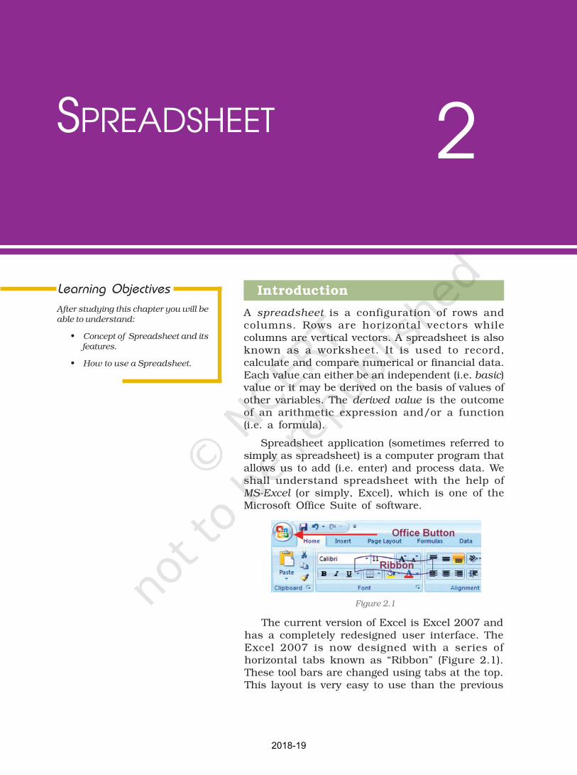
The current version of Excel is Excel 2007 andhas a completely redesigned user interface. TheExcel 2007 is now designed with a series ofhorizontal tabs known as “Ribbon” (Figure 2.1).These tool bars are changed using tabs at the top.This layout is very easy to use than the previous
Figure 2.1
2018-19

18
Computerised Accounting System
versions of Excel. On clicking with left button of mouse at
“Office Button” ; we will be able to open an old workbook or create
a new one or can save the workbook or can print which were earlieravailable in previous version of Excel in File menu.
2.1 BASIC CONCEPTS OF SPREADSHEET
A file in Excel is known as a “Workbook”. A workbook is a collection ofa number of “Worksheets” (Figure 2.2). By default, three sheets, namelySheet 1, Sheet 2, and Sheet 3 are available to users. At a time, onlyone worksheet can be made as “Active Worksheet” and that worksheetis available to a user for carrying out operations. An active worksheet’sname will be shown in bold letters in the “Sheet Tab” at the bottom leftof the screen. Additional sheets can be added, if required, by clicking
on the icon (which works as Insert ! W ! W ! W ! W ! Worksheetorksheetorksheetorksheetorksheet).
The Sheet names can bechanged, if required, by right-clicking the mouse over the Sheet1or Sheet 2 or Sheet 3 after selectingand pointing it on the sheet name(which is to be changed) and selec-ting “Rename” option.
Box 2.1Box 2.1Box 2.1Box 2.1Box 2.1
Basic and Derived VBasic and Derived VBasic and Derived VBasic and Derived VBasic and Derived Valuesaluesaluesaluesalues
If quantity (Q) of an item is
purchased at a price (P), the value
of that item (V) is derived as
follows:
V = Q × P
Here, the values P and Q are
Basic Values. While V is the
Derived Value as it is obtained
by multiplying Q with P. The
expression (Q×P) is called as
arithmetic expression. Addi-
tional examples of arithmeticexpressions are given later in this
chapter.
Note: In general, an arithmeticexpression may contain one or
more functions.Figure 2.2
2018-19

Spreadsheet
19
Figure 2.3
RowsRowsRowsRowsRows are numbered numericallyfrom top to bottom while ColumnsColumnsColumnsColumnsColumnsare referred by alpha charactersfrom left to right. In Excel 2007,there are 65536 RowsRowsRowsRowsRows which arenumbered as 1, 2, 3, … 65,536. Thesenumbers are shown on the left mostportion of the worksheet. ColumnsColumnsColumnsColumnsColumns(total 256 in Excel) are identifiedby letters, such as A, B, C,.. AA…IV, and are shown on the horizontalbox just above Row 1. Thus, thereare 65,536 256 = 1,65,00,000,approximately cells, which is indeed a huge work area, sufficient forall application requirements (Figure 2.3) in one sheet.
In a spreadsheet, a value or function or an arithmetic expression isrecorded in a cellcellcellcellcell. The intersection of a rowrowrowrowrow and a columncolumncolumncolumncolumn is called acell. cell. cell. cell. cell. A cellcel lcel lcel lcel l is identified by a combination of a letter and a numbercorresponding to a particular location within the spreadsheet. Forexample, the first cell of a worksheet is identified as A1 as it shown inFigure 2.2 at row 1 and column (A). When we start Excel, the pointer(cursor) points to the first cell, i.e. A1, and this cell is called the ActiveActiveActiveActiveActiveCellCellCellCellCell. We can move around a worksheet through four arrow keys (i.e.left, right, up, down as shown in Figure 2.4). For example, the cellhaving address as G8 correspond to 8th row under G column. Eachcell thus has a unique identification called as cell addresscell addresscell addresscell addresscell address.
Cell Reference — — — — — A cell reference identifies the location of a cell orgroup of cells in the spreadsheet also referred as a cell address. Cellreferences are used in formulas, functions, charts, other Excelcommands and also refer to a group or range of cells. RangesRangesRangesRangesRanges areidentified by the cell references of the cells in the upper left (cell A1)and lower right (cell E2) corners in Figure 2.3. The ranges are identifiedusing colon (:) e.g. A1: E2 which tells Excel to include all the cellsbetween these start and end points. By default cell reference isrelative; which means that as a formula or function is copied andpasted to other cells, the cell references in the formula or functionchange to reflect the new location. The other cell reference is absolutecell reference which consists of the column letter and row numbersurrounded by dollar ($) signs e.g. $C$4. An absolute cell reference isused when we want a cell reference to stay fixed on specific cell,which means that when a formula or function is copied and pasted toother cells, the cell references in the formula or function do not change.A mixed reference is also a cell reference that holds either row orcolumn constant when the formula or function is copied to anotherlocation e.g., $C4 or C$4.
2018-19

20
Computerised Accounting System
The mouse is used for all the operations requiredand for navigation in worksheet (or workbook) exceptdata entry; but some of the important operations andcommon navigations can be performed by using keystrokes (as given below). It is better to understandand know all the keys of keyboard and key strokes.Pressing a key is called key stroke but to fulfill onecommand for operation in the worksheet some timewe require pressing two keys together to get one keystroke (Figure 2.4)
MovementMovementMovementMovementMovement Key Stroke (Press key)Key Stroke (Press key)Key Stroke (Press key)Key Stroke (Press key)Key Stroke (Press key)
One cell down Down arrow key ( ) or EnterEnterEnterEnterEnter key
One cell up Up arrow key ( )
One cell left Left arrow key ( )
One cell right Right arrow key ( ) or TabTabTabTabTab key
The other navigational and operational strokes are used for fastercursor movement than one cell at a time with cluster of filled cells.Cluster of filled cells implies a set of consecutive cells in a row or in acolumn having some data.
Figure 2.4
The data that is entered in a cell may be either numeric or alpha-numeric or a date. As a data is typed in a cell, Excel is able to makeout its type (i.e. numeric or alpha-numeric or date) depending on thenature of value typed in a cell.
MovementMovementMovementMovementMovement Key Stroke (Press key)Key Stroke (Press key)Key Stroke (Press key)Key Stroke (Press key)Key Stroke (Press key)
Top of Worksheet (cell A1) CTRLCTRLCTRLCTRLCTRL + HOMEHOMEHOMEHOMEHOME (i.e. Keep CTRLCTRLCTRLCTRLCTRL keypressed and then press HOMEHOMEHOMEHOMEHOME key
The cell at the intersection of the CTRLCTRLCTRLCTRLCTRL + ENDENDENDENDEND keyslast row and last column containing data
Moving consecutively to the first and the last CTRLCTRLCTRLCTRLCTRL + Right arrow key ( ) orfilled cells of clusters of filled cells in a row by else ENDENDENDENDEND + Right arrow key ( )successive pressing of CTRLCTRLCTRLCTRLCTRL + Right arrowkey ( ) or else ENDENDENDENDEND + Right arrow key ( )
Moving consecutively to the first and the last CTRLCTRLCTRLCTRLCTRL + Down arrow key ( ) orfilled cells of a cluster of filled cells in a column else ENDENDENDENDEND + Down arrow key ( )by successive pressing of CTRLCTRLCTRLCTRLCTRL + Down arrowkey ( ) or else ENDENDENDENDEND + Down arrow key ( )
Beginning of the Row HOMEHOMEHOMEHOMEHOME key
Beginning of the Column
Navigating In (i.e. Moving arNavigating In (i.e. Moving arNavigating In (i.e. Moving arNavigating In (i.e. Moving arNavigating In (i.e. Moving around) The Wound) The Wound) The Wound) The Wound) The Worksheetorksheetorksheetorksheetorksheet
2018-19
Spreadsheet
21
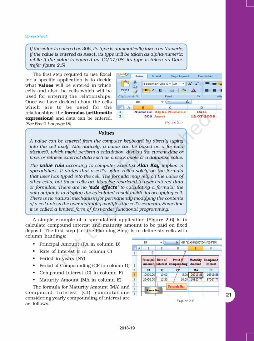
If the value is entered as 306, its type is automatically taken as Numeric;if the value is entered as Asset, its type will be taken as alpha-numeric;while if the value is entered as 12/07/08, its type is taken as Date.(refer figure 2.5)
The first step required to use Excelfor a specific application is to decidewhat values will be entered in whichcells and also the cells which will beused for entering the relationships.Once we have decided about the cellswhich are to be used for therelationships; the formulas (arithmeticexpressions) and data can be entered.(See Box 2.1 at page18)
VVVVValuesaluesaluesaluesalues
A value can be entered from the computer keyboard by directly typinginto the cell itself. Alternatively, a value can be based on a formula(derived), which might perform a calculation, display the current date ortime, or retrieve external data such as a stock quote or a database value.
The value rulevalue rulevalue rulevalue rulevalue rule according to computer scientist Alan KayAlan KayAlan KayAlan KayAlan Kay implies inspreadsheet. It states that a cell’s value relies solely on the formulathat user has typed into the cell. The formula may rely on the value ofother cells, but those cells are likewise restricted to user-entered dataor formulas. There are no ‘side ef‘side ef‘side ef‘side ef‘side effects’fects’fects’fects’fects’ to calculating a formula: theonly output is to display the calculated result inside its occupying cell.There is no natural mechanism for permanently modifying the contentsof a cell unless the user manually modifies the cell’s contents. Sometimeit is called a limited form of first-order functional programming.
A simple example of a spreadsheet application (Figure 2.6) is tocalculate compound interest and maturity amount to be paid on fixeddeposit. The first step (i.e. the Planning Step) is to define six cells withcolumn headings:
• Principal Amount (PA in column B)
• Rate of Interest (r in column C)
• Period in years (NY)
• Period of Compounding (CP in column D)
• Compound Interest (CI in column F)
• Maturity Amount (MA in column E)
The formula for Maturity Amount (MA) andCompound Interest (CI) computationsconsidering yearly compounding of interest areas follows:
Figure 2.5
Figure 2.6
2018-19
22
Computerised Accounting System
MA = PA * (1 + R / (100 * CP)) ^ (R * CP)CI= MA – PA
Now, we can decide the layout of the worksheet for (compound)interest calculation as shown in Figure 2.6.
It may be observed that the basic values are entered in cells (as infigure 2.6 the cells are B4, C4 and D4); the derived values (as in Figure2.6 the cells are E4 and F4) are automatically computed (using aboveformula) and shown in forforforforformula barmula barmula barmula barmula bar. In case any basic values aremodified, the derived values as a result are revised accordingly. Thisfeature of Spreadsheets enables us to study various what-if scenarioswhat-if scenarioswhat-if scenarioswhat-if scenarioswhat-if scenarios.
A what-if scenariowhat-if scenariowhat-if scenariowhat-if scenariowhat-if scenario is used to generate a number of alternatives toexamine the cause (if) and effect (what). Thus, it helps in analysing theimpact of changes due to variations in one or more input values. Takingthe above example, if all the other values are kept same, one can seehow different rates of interest and different periods of compoundingwould affect the Compound Interest and the Maturity Amount to bereceived.
Before proceeding further for the above example we have tounderstand some of the basic terminologies and features of thespreadsheet such as:
2.1.1 LABELS
A text or especial character will be treated as labels for rows or columnsor descriptive information. Labels cannot be treated mathematically-multiplied, subtracted, etc. Labels include any cell contents beginningwith A-Z e.g., in the above Figure 2.6 Principal Amount, Rate ofInterest, Maturity amount, etc. will be taken as labels.
2.1.2 FORMULAS
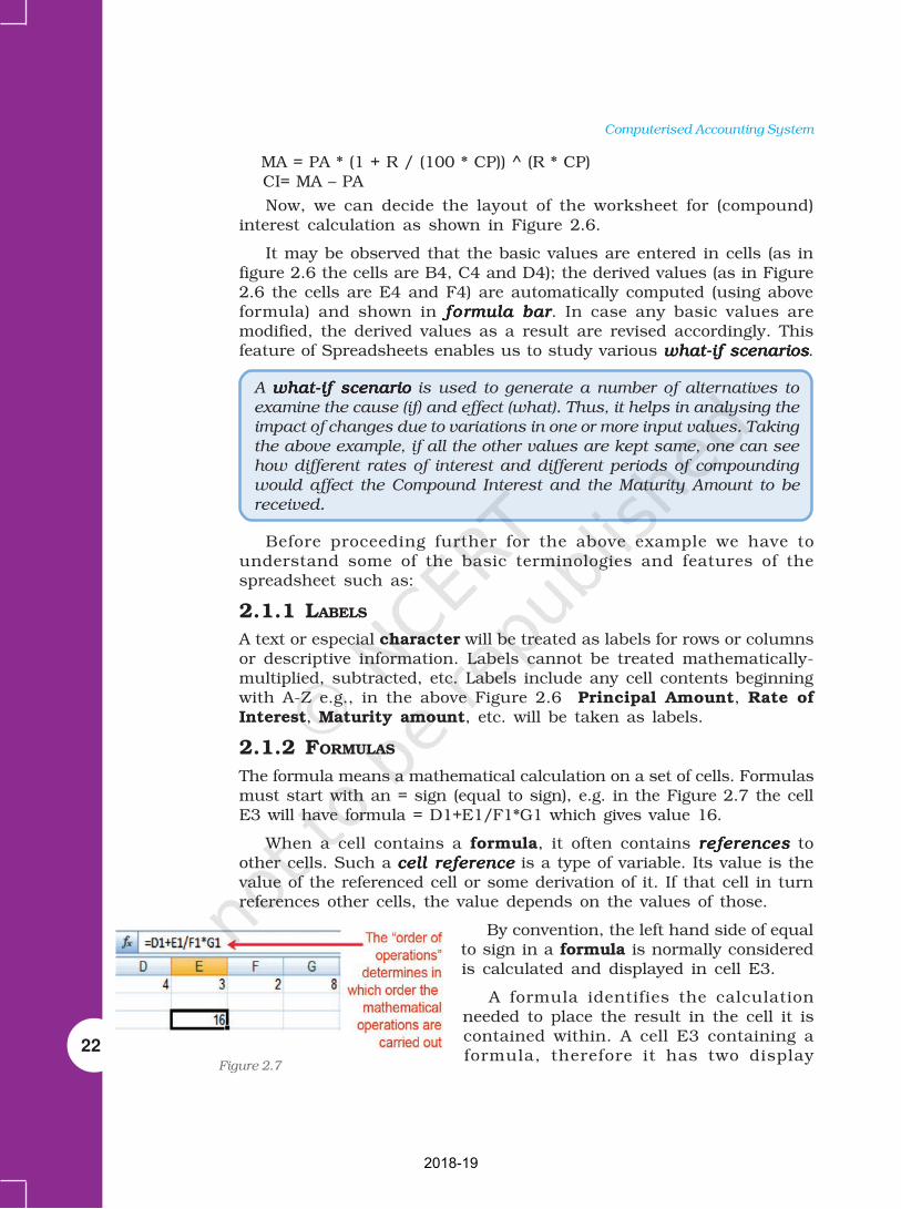
The formula means a mathematical calculation on a set of cells. Formulasmust start with an = sign (equal to sign), e.g. in the Figure 2.7 the cellE3 will have formula = D1+E1/F1*G1 which gives value 16.
When a cell contains a formula, it often contains referencesreferencesreferencesreferencesreferences toother cells. Such a cell referencecell referencecell referencecell referencecell reference is a type of variable. Its value is thevalue of the referenced cell or some derivation of it. If that cell in turnreferences other cells, the value depends on the values of those.
By convention, the left hand side of equalto sign in a formula is normally consideredis calculated and displayed in cell E3.
A formula identifies the calculationneeded to place the result in the cell it iscontained within. A cell E3 containing aformula, therefore it has two display
Figure 2.7
2018-19

Spreadsheet
23
components; the formula itself and the resulting value. The formula isshown only when the cell is selected by “clicking” the mouse over aparticular cell; otherwise it contains the result of the calculation (inthis case 16).
The arithmetic operations and complex nested conditional (what-(what-(what-(what-(what-if scenario)if scenario)if scenario)if scenario)if scenario) operations can be performed by spreadsheets which followorder oforder oforder oforder oforder of mathematical (expression) operations rulesmathematical (expression) operations rulesmathematical (expression) operations rulesmathematical (expression) operations rulesmathematical (expression) operations rules.
A spreadsheet without any formulas is a collection of data whichare arranged in rows and columns (a database) like a calendar, timetableor simple list, etc. There is a Formula tab on Excel ribbon (Figure2.8(a) which contains four sections, functions library, defined names,formula auditing and calculation.
2.1.3 FUNCTIONS
A function is a special key word which can be entered into a cell inorder to perform and process the data which is appended withinbrackets.
Figure 2.8(a)
Order of mathematical operations (expressions)
Computer math uses the rules of Algebra..... Any operation(s) contained in bracketswill be carried out first followed by any exponents.
After that, Excel considers division or multiplication operations to be of equalimportance, and carries out these operations in the order they occur left to rightin the equation.
The same goes for the next two operations – addition and subtraction. They areconsidered equal in the order of operations. Whichever one appears first in anequation, either addition or subtraction is the operation carried out first.
Three easy ways to remember the order of operations is to use the acronym:
GEMS PEMDAS BEMDAS
( ) Grouping Please - ( )parenthesis ( ) Brackets
^ Exponents Excuse - ^ exponents ^ Exponents
* Multiplication : My - * multiply * Multiplication/ or Division : Dear - / divide / Division
- Subtraction : Aunt - + add + Addition+ or Addition : Sally - - subtract - Subtraction
2018-19

24
Computerised Accounting System
There is a function button on the formula toolbar (fffffx) (figure 2.8(b);when we click with the mouse on it; a function offers assistance anduseful prompts into a spreadsheet cell. Alternatively we can enter thefunction directly into the formula bar. A function involves four mainissues:
• Name of the function
• The purpose of the function
• The function needs whatargument(s) in order tocarry its assignment.
• The result of the function.
A function is a built in set of formulas which starts with an =“equal to sign” such as = FunctionName(Data). The data (or argumentin proper terminology) includes a range of cells.
SUM (), AVERAGE () and COUNT () are common functions andrelatively easy to understand. They each apply to a range of cellscontaining numbers (or blank but not text) and return either thearithmetic total of the numbers, the average mean value or the quantityof values in the range.
For Example: The SUM or AutoSum () function is the most basicand one of the common user functions. It is used to get the addition of
various numbers or the contents of various cells. On the ribbon (Figure2.9(a)) the AutoSum () button can be use directly for summation ofvalues from cells. Once we click the AutoSum () at cell H1, the functionadds the contents of cell range D1 to G1 and displays the answer thatwe want to get the sum of. If we want answer in the cell G5 (Figure2.9(b) use the mouse to click in the cell G5 and click AutoSum buttonthen from keyboard type range of the cells D1:G1; the answer 17 willappear in cell G5; or we can write directly the complete function =SUM (D1: G1) appears in the formula bar above the worksheet. TheAutoSum function also includes other series based functions such asAVERAGE, MIN, MAX and COUNT.
Figure 2.8(b)
Figure 2.9(a) Figure 2.9(b)
2018-19

Spreadsheet
25
There are twelve different categories of functions available in Excel2007 displayed on the ribbon (Figure 2.8) which are classified as perthe usage e.g. The Financial, Date and Time, Lookup and References,Database, Text and Logical functions are useful in ComputerisedAccountancy and will be explained later subsequently.
Naming Ranges – IF Functions – Nested IF Functions
As mentioned earlier, we will now learn the arithmetic operations andcomplex nested conditional (what-if scenario)(what-if scenario)(what-if scenario)(what-if scenario)(what-if scenario) using name ranges,absolute cell references and mixed references in following sections.
Naming Cells and Ranges
Naming ranges in Excel will save time forwriting complex formulas. The name can beused in place of cell range whenever referenceit e.g. in D3 we have = SUM (B1:F1)(Figure 2.10)
The cell referenced in the function B1:F1can be replaced with a descriptive namesay NumbersNumbersNumbersNumbersNumbers (name range) which iseasier to remember and in D3 it will be= SUM (Numbers)
Behind the Numbers Numbers Numbers Numbers Numbers Excel is hiding cell references, we will see howit works now.
The steps are for defining Name Ranges are asfollows:
1. Select the cell(s) which are to be named(such as B1:F1 in Figure 2.10(a)).
2. Click on the ribbon on formula tab.
3. Select Define Name (Figure 2.10(b) optionon the ribbon and click it.
4. This will provide a dialogue box will beopened as shown in Figure 2.10(c) to clickDefine Name (another option Apply Names is for previously createdRange Names to select) (Figure 2.10(d)).
Figure 2.10
Figure 2.10(a)
Figure 2.10(b) Figure 2.10(c)
2018-19

26
Computerised Accounting System
5. This will display a dialogue box as NewName shown in Figure 2.10(d). It willprovide a window “Name” in which type“Numbers” which will represent cellranges $B$1:$F$1 as shown in be“Refers to” window.
6. Click OK on the New Name dialogue boxwhich returns to the spreadsheet. Noticethat the Name Box having our heading“Numbers”.
7. To apply this name in cell D3 for summation fromB1:F1 click on Apply Name and a dialogue box willbe opened then click on a Name Range – Numbers(Figure 10(e)). The D3 will be having =SUM (Numbers)And will display the result (Figure 10(f)). The namedrange can be used with other Functions such asAVERAGE (), SUMIF () etc.
Now we will use a summation of numbers using conditionin the cell D3. Type the formula = SUMIF (Numbers,”<6)and the answer will be 9 (for the Numbers less than 6 inthe named range B1:F1) (Figure 2.10(f)).
Let us understand with the help of anotherexample in which we will be using two Named Ranges(Figure 2.11) namely Monthly_Totals for cells B2:B5
Figure 2.10(d)
Figure 2.10(f)
Figure 2.10(e)
Figure 2.10(g)
Figure 2.11
and Monthly_Tax for cells C2:C5respectively created as described above.
The cell B6 will have value 1158by using function as =SUM(Monthly_Totals).
Similarly in Figure 2.11(a) if weuse Autosum Function () from theformula tab of the ribbon at the cellC6; the function will include theNamed Ranges as an argument andgives the result 238.
2018-19

Spreadsheet
27
We will now use these two NamedRanges to calculate the Balance (in cellB7) after using the formula tax frommonthly totals. Let us giveTotal_of_Month is the Named Range forcell B6 and similarly, the Total_of_Taxis the Named Range for cell C6. With thesetwo Named Ranges; the cell B7 will havethe difference of these two amounts andwill be written (Figure 2.11(b)) as= Total_of_Month – Total_of_Tax .
To prevent its recalculation andmaintain the present calculated value asshown in the cells B6, C6 and B7respectively (Figure 2.11(b) we can freezethe formula using Paste Specialcommand. The following steps arerequired:
1. Select the cell (s) that contains theformula e.g. B6:C6, B7 (Figure 2.11(b)
2. Click on Home Tab and select Copysymbol (Figure 2.11(c)) to click, thiswill copy the values and formulas ofthe cells (Figure 2.11(d)).
3. Click on Paste tab and select PasteSpecial.
4. In the Paste Special box (Figure 2.11(d)), under paste select the radiobutton next to Values and click OK.This will permanently remove theformula from the workbook.
In continuation to our need of what-if-scenario now we will learn about animportant logical function IF Function.This function can be evoked from formulatab on the ribbon. This function returnsone value if a specified condition evaluatedto TRUE and another value if it evaluatesto FALSE. We will learn more about theusage of functions in the businessapplications subsequently; there are alarge selection of if functions available.An IF function has the following format:
IF (logical_test, value_if_ture,value_if_false) where
Figure 2.11(a)
Figure 2.11(b)
Figure 2.11(c)
Figure 2.11(d)
2018-19

28
Computerised Accounting System
logical_test : the value or expression that is determined to be true orfalse; this requires the usage of a logical operator. A logical operator isone used to perform a comparison between two values and produce aresult of true or false (there is no middle result: something is not halftrue or half false or “Don’t Know”; either it is true or it is false). Forexample, A1 < 20 could be used as a logical test, where symbol “<“ is alogical operator “less than”. (There are many more logical operatorssuch as =, <=, <>, >, >= etc.)
value_if_true : The value returned if the test is determined to be true.This value can be a value, text, or expression, formula, etc. or it can bereturn the value of another cell.
value_if_false : The value returned, if the test is determined to befalse. This value can be a value, text, or expression, formula, etc. or itcan return the value of another cell.
e.g. i. = IF( A1 < 20, “Yes”, “No”) this function will return Yes if cellA1 < 20 and o for anything else.
ii. = IF (C2 > B2, (C2+D2)/2, (B2+D2)/2) this function will compareboth cell C2 > B2 and will calculate and return (C2+D2)/2 if itis true else it will calculate and return (B2+D2)/2.
Example : Let us calculate the amount of saving (Cell address ”value”) onthe basis of percentage value (Cell address “saving”) shown in figure 2.12(a)
Creating IF function using the Formula Tab and dialogue box.
1. Select the cell F4 (Figure 2.12(a) where the function is to be introduce
2. Click at the Formula tab on the ribbon and click logical option.
3. Select IF function which will provideFunction Arguments dialogue box(Figure 2.12(b).
4. Type an appropriate condition in thelogical_test box ( e.g. E4 > 10000 )
5. In the value_if_true box type therequire value (e.g. 10%) if the logicaltest condition is met.
6. In the value_if_false box type thevalue (e.g. 5%) if the logical testcondition is NOT met.
7. Click OK, the answer for thecondition will be displayed (in cellF4 it will be 5%). Copy the functionfrom F4 to all other cells F5:F11.
In the Formula Box the function will be displayed as
=IF (F4>10000, 10%, 5%)
This is simple use of IF function. The nested IFs can be used tolook for several conditions and to look at different types of functions.
Figure 2.12(a)
2018-19

Spreadsheet
29
e.g. = IF (AVERAGE (A2:A6) > 10, SUM(B2:B6), 0)
This function will be able to look atthe average of cells A2 to A6 and if theaverage is higher than 10 it will sumthe value of the cells B2 to B6, if theaverage is equal to or less than 10 itwill return to 0.
In some cases, we need to checkmore than one condition. In otherwords, check the first condition; if thatcondition is false, check anothercondition. If a nested function is used as an argument it must returnthe same type of value that the argument uses. For example, if theargument returns a TRUE or FALSE value, then the nested functionmust return a TRUE or FALSE otherwise MS Excel will display anerror message #Value! in the cell.
This way we can check as many conditions as we need to. Thetruthfulness of each condition would lead to its own statement. If noneof the conditions is true, then it executes the last statement. Toimplement this scenario include an IF() function inside of another.Such as :
= IF (logical_test, value_if_true, value_if_false) simple if statement.
Let us substitute other IFs
IF (logical_test, IF (logical_test, IF (logical_test, value_if_true,value_if_false), value_if_false), value_if_false)
e.g. Suppose E2 cell contains marks of a test and cell F2 will haveresult based on following nested IF () condition.
= IF (E2<96, IF (E2<91, IF (E2<55,”Fail”,”C Grade”), “B Grade”),“A Grade”)
2.1.4 OTHER USEFUL FUNCTIONS
In business applications the inputof data usually contains dates (dateof invoice preparation, date ofpayment, payment received date, ordue date etc.), rate of interest, taxpercentage and output informationmay require age calculation,duration, delays in payment,accumulated interest, depreciation,future value, net present value, etc.
The MS Excel provides library ofsuch functions in which input data
Figure 2.12(b)
Figure 2.13
2018-19

30
Computerised Accounting System
can be worked as arguments and result available from the functionwill be output information. On the ribbon of MS Excel, the formula tabcontains categorised function libraries (Figure 2.13).
a. Date and Time Function.
b. Mathematical Function.
c. Text Manipulation function.
d. Logical Function (other than IF).
e. Lookup and Reference Function.
f. Financial Function.
The complete details of each function from arange of above categories including examples areavailable through Help (?) on the Ribbon. Thequickest way to get help on a function whose name(e.g. SUMIF) when we entered on formula barfollowed by equal to sign then double-click the
function’s name that appears in the strip (as shown in the figure 2.14).We will learn some of the useful function with the help of examples.
2.1.4.1 Date and Time Function
1. TODAY () is the function for today’s date in the blank worksheet.
TODAY – Returns the serial number of the current date. The serialnumber is the date-time code used by Excel for date and timecalculations. Times are represented as fractions of a day. By defaultJanuary 1, 1900 is serial number 1. Thus, January 1, 2009 is serialnumber 39814 (because it is 39814 days after January 1, 1900).
2. NOW () is similar function but it includes the current time also(Figure 2.15).
3. DAY(serial_number) function returns the day of a date as an integerranging from1 to 31. For example, if A5 = 16-Apr-2009 then = DAY (A2)will be 16. Similarly, two other functions MONTH(serial_number)returns month of a date as an integer ranging from 1 (January) to 12(December) (Figure 2.16) and YEAR(serial_number) returns the yearcorresponding to a date as an integer ranging from 1900 – 9999.
4. DATEVALUE (date_text) converts a date in the form of text to aserial number e.g. =DATEVALUE(“16-04-2009”) will return a value39919.
Figure 2.14
Figure 2.15 Figure 2.16
2018-19

Spreadsheet
31
Example: To find out the age of an employeeas on today is a very simple mathematicalcalculation in the spreadsheet, e.g. the ageof a person on 16-Apr-2009 whose Date ofBirth is 16-Apr-1980 can be calculated asper Figure 2.17. The difference of two dates(in D3) is divided by 365.25 to convert daysinto years (considered the fractional valuefor leap years).
2.1.4.2 Mathematical Function
In business applications some of theMathematical Functions are very useful,such as:
1. SUMIF is the function which adds the cells as per given specifiedcriteria the syntax of this is as follows:
SUMIF (range, criteria, sum_range) where
Range it is the range of cells to evaluate.
Criteria it is the criteria in the form of anumber, expression, or text that defines whichcells will be added, e.g. criteria can beexpressed 1500, “1500”, “>1500” or “Books”.
Sum_range are the actual cells to sum.
e.g. There are sum Asset Values (D2:D5)and related to each asset values thereare deprecation values (E2:E5). UsingSUMIF function we have to calculate thesum of depreciation for those Asset Values which are more than 1,70,000/-.The function is written in the cell E7 like =SUMIF (D2:E5,”>150000,E2:E5) which gives result 63,000/- (Figure 2.18)
2. ROUND is the function to rounds a number to specified number ofdigits. The syntax of this function is as follows:
ROUND (number, num_digits) where
Number Is the number to round (preferablyfractional number)
Num_digits specifies the number of digits toround the Number. There may be somedifferent situations for Num_digits as follows:
a. If Num_digits is greater than 0 (zero),then number is rounded to the specifiednumber of decimal places.
b. If Num_digits is 0, then number isrounded to the nearest integer.
Figure 2.17
Figure 2.18
Figure 2.19
2018-19

32
Computerised Accounting System
c. If Num_digits is less than 0, then number is rounded to the left ofthe decimal point.
ExaExaExaExaExamplemplemplemplemple - refer Figure 2.19
i. to round the number 21.5 by 1 digit ( result is 2.2)
ii. to round the number 2.149 by 1 digit ( result is 2.1)
iii. to round the number -1.475 by 2 digits ( result is -1.48)
vi. to round the number 21.5 by -1 digit ( result is 20.0)
To round a number to the nearest whole number because decimalvalues are not significant or round a number to multiples of 10 tosimplify an approximation of amounts. There are several ways to rounda number other than ROUND are:
ROUNDUP (number, num_digits) which rounds a number up, awayfrom 0 (zero) e.g.
= ROUNDUP (3.2, 0) Rounds 3.2 up to zero decimalplaces and the value is 4.
= ROUNDUP (76.9, 0) Rounds 76.9 up to zero decimalplaces and value is 77.
= ROUNDUP (3.14159, 3) Rounds 3.14159 up to threedecimal places; value 3.142.
= ROUNDUP (-3.14159, 1) Rounds -3.14159 up to onedecimal place; value -3.2.
= ROUNDUP (31415.92654,-2) Rounds 31415.92654 up to 2decimal places to the left of thedecimal; value 31500.
ROUNDDOWN (number, num_digits) which rounds a number down,toward zero.
= ROUNDDOWN (3.2, 0) Rounds 3.2 down to zero decimalplaces; value 3.
= ROUNDDOWN (76.9, 0) Rounds 76.9 down to zerodecimal places; value 76.
= ROUNDDOWN (3.14159, 3) Rounds 3.14159 down to threedecimal places; value 3.141.
= ROUNDDOWN (-3.14159, 1) Rounds -3.14159 down to onedecimal place; value -3.1.
= ROUNDDOWN (31415.92654, -2) Rounds 31415.92654 down to 2decimal places to the left of thedecimal; value 31400.
3. COUNT
This function counts the number of cells that contain numbers andcounts numbers within the list of arguments. COUNT is use to get thenumber of the entries in a number field (including date also) i.e. in arange or array of numbers.
2018-19

Spreadsheet
33
In Excel other than counting function COUNT; other functions areCOUNTA, COUNTBLANK, and COUNTIF —which enable us to count the number ofcells that contain values, are nonblank (andthus contain entries of any kind), or countonly the cells in a given range that meetthe user defined criteria.
The syntax for COUNT is COUNT (value1,value2…..,) where value1, value2, ... are1 to 255 arguments that can be a varietyof different types of data(logical valuesrepresented in numbers, numbers, dates,or text representation of numbers), but onlynumbers are counted.
Arguments that are error values or textthat cannot be translated into numbers are ignored.
If an argument is an array or reference, only numbers in that array orreference are counted. Empty cells, logical values, text, or error valuesin the array or reference are ignored.
COUNTA function will be count logical values, text, or error values.The Figure 2.20 contains a named range for cells A1:B9 as Count_Data
There are other functions also such as ROWS and COLUMNS are used.The syntax is as follows:
ROWS (array)
The function returns the number of rows in a reference or array; wherean Array is an array, an array formula or a reference to a range ofcells for which we want the number of rows.
COLUMNS (array)
This function returns the number of columns in an array or namedrange reference; where an Array is an array or array formula or areference to a range of cells for which we want the number of columns.
Figure 2.20
ArrayArrayArrayArrayArray: Used to build single formulas that produce multiple results or that operate ona group of arguments that are arranged in rows and columns. An array range sharesa common formula; an array constant is a group of constants used as an argument.
Array forArray forArray forArray forArray formulamulamulamulamula: A formula that performs multiple calculations on one or more sets ofvalues, and then returns either a single result or multiple results. Array formulas areenclosed between braces { } and are entered by pressing CTRL+SHIFT+ENTER.CTRL+SHIFT+ENTER.CTRL+SHIFT+ENTER.CTRL+SHIFT+ENTER.CTRL+SHIFT+ENTER.
COUNTIF (range, criteria) (Figure 2.21)
This function counts the number of cells within a range that meet thegiven criteria; in this function the Range is one or more cells to count,including numbers or names, arrays, or references that containnumbers. The blank cells and text values are ignored. (e.g. A2:B5)
2018-19

34
Computerised Accounting System
Criteria are the form of a number, expression,cell reference, or text that defines which cellswill be counted. For example, criteria can beexpressed as 32, “32”, “>32”, “apples”, or B4.
2.1.4.3 Text Manipulation Function
1. TEXT
This function converts a numeric value to textin a specific number format; and the syntax is :
TEXT (value, format_text) where,
Value is a numeric value, a formula that evaluates to anumeric value, or a reference to a cell containing a numeric value.
Format_text is a numeric format as a text string enclosed in quotationmarks. We can see various numeric formats by clicking the Number,Date, Time, Currency, or Custom in the Category box of the Numbertab in the Format Cells dialog box, and then viewing the formatsdisplayed.
This function is useful in situations where we want to displaynumbers in a more readable format, or want to combine numbers withtext or symbols. For example, suppose cell L1 contains the number23.5. Suppose we want to format this number by adding with “Rs.”and convert into amount using this function:
=TEXT L1,”Rs. 0.00") which will be displayed as Rs. 23.50 (Figure2.22).
We can also format numbers by using thecommands in the Number group on the Hometab of the Ribbon. However, these commands workonly if the entire cell is numeric. Refer Figure2.22(a); you will find in cell A5(A6) usingfunction combined with ‘$’ sign which can be
used with other functions (such as logical).
2. CONCATENATE
This function joins two or more text strings into one text string and its syntax is:
CONCATENATE (text1,text2,...) where
text1, text2, …. are 2 to 255text items to be joined into asingle text item. The text itemscan be text strings, numbers, orsingle-cell references.
Example combining First Name,
Figure 2.21
Figure 2.22
Figure 2.22(a)
2018-19
Spreadsheet
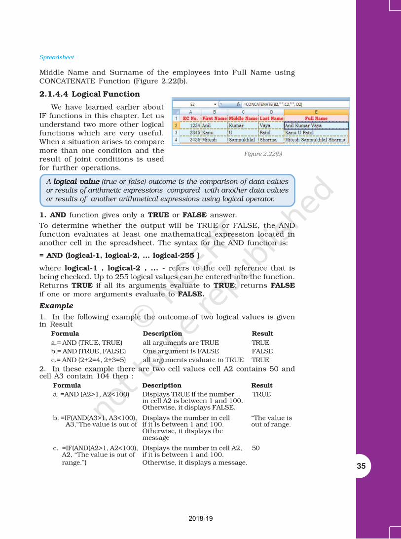
35
Middle Name and Surname of the employees into Full Name usingCONCATENATE Function (Figure 2.22(b).
2.1.4.4 Logical Function
We have learned earlier aboutIF functions in this chapter. Let usunderstand two more other logicalfunctions which are very useful.When a situation arises to comparemore than one condition and theresult of joint conditions is usedfor further operations.
Figure 2.22(b)
1. AND function gives only a TRUE or FALSE answer.
To determine whether the output will be TRUE or FALSE, the ANDfunction evaluates at least one mathematical expression located inanother cell in the spreadsheet. The syntax for the AND function is:
= AND (logical-1, logical-2, ... logical-255 )
where logical-1 , logical-2 , ... - refers to the cell reference that isbeing checked. Up to 255 logical values can be entered into the function.Returns TRUE if all its arguments evaluate to TRUE; returns FALSEif one or more arguments evaluate to FALSE.
ExampleExampleExampleExampleExample
1. In the following example the outcome of two logical values is givenin Result
Formula Description Result
a.= AND (TRUE, TRUE) all arguments are TRUE TRUE
b.= AND (TRUE, FALSE) One argument is FALSE FALSE
c.= AND (2+2=4, 2+3=5) all arguments evaluate to TRUE TRUE
2. In these example there are two cell values cell A2 contains 50 andcell A3 contain 104 then :
Formula Description Result
a. =AND (A2>1, A2<100) Displays TRUE if the number TRUEin cell A2 is between 1 and 100.Otherwise, it displays FALSE.
b. =IF(AND(A3>1, A3<100), Displays the number in cell “The value is A3,“The value is out of if it is between 1 and 100. out of range.
Otherwise, it displays themessage
c. =IF(AND(A2>1, A2<100), Displays the number in cell A2, 50A2, “The value is out of if it is between 1 and 100.range.”) Otherwise, it displays a message.
A logical valuelogical valuelogical valuelogical valuelogical value (true or false) outcome is the comparison of data valuesor results of arithmetic expressions compared with another data valuesor results of another arithmetical expressions using logical operator.
2018-19

36
Computerised Accounting System
One common use for the AND function is to expand the usefulness ofother functions that perform logical tests.
In the above example, the IF function performs a logical test and thenreturns one value if the test evaluates to TRUE and another value if thetest evaluates to FALSE. By using the AND function as the logical_test logical_test logical_test logical_test logical_testargument of the IF function, we can test many different conditions.
2. OR function is like other logical functions, the OR function givesonly a TRUE or FALSE answer. To determine whether the output willbe TRUE or FALSE, the OR functions evaluates at least onemathematical expression located in another cell in the spreadsheet.This function returns TRUE if any argument is TRUE; returns FALSEif all arguments are FALSE.
The syntax for the OR function is:
= OR (logical-1, logical-2, ... logical-255 )
Logical-1, logical-2 … - refers to the cell references that are beingchecked. Up to 255 logical values can be entered into the function.
ExampleExampleExampleExampleExample
Formula Description Result
a.= OR (TRUE, FALSE) One argument is TRUE TRUE
b.=OR ((1+1)=1,(2+2)=5) All arguments evaluate to FALSE FALSE
c.=OR (TRUE,FALSE,TRUE) At least one argument is TRUE TRUE
2.1.4.5 Lookup and References Function
The LOOKUP function returns a value either from a one-row or one-column range or from an array. The LOOKUP function has two syntaxforms: vector and array.
The Look Up function can be used as an alternative to the IF functionfor elaborate tests or tests that exceeds the limit for nesting of IFfunctions.
The vector forvector forvector forvector forvector formmmmm of LOOKUPLOOKUPLOOKUPLOOKUPLOOKUP looks in a one-row or one-column range (known as avector) for a value, and then returns a value from the same position in a second one-row or one-column range.
The array forarray forarray forarray forarray formmmmm of LOOKUPLOOKUPLOOKUPLOOKUPLOOKUP looks in the first row or column of an array for thespecified value, and then returns a value from the same position in the last row orcolumn of the array.
1. LOOKUP 1. LOOKUP 1. LOOKUP 1. LOOKUP 1. LOOKUP (Vector Form)
The syntax is LOOKUP (lookup_valuelookup_valuelookup_valuelookup_valuelookup_value, lookup_vectorlookup_vectorlookup_vectorlookup_vectorlookup_vector, rrrrresult_vectoresult_vectoresult_vectoresult_vectoresult_vector)
• Lookup_value is a value that LOOKUP searches for in the firstvector. Lookup_value can be a number, text, a logical value, or aname or reference that refers to a value.
2018-19
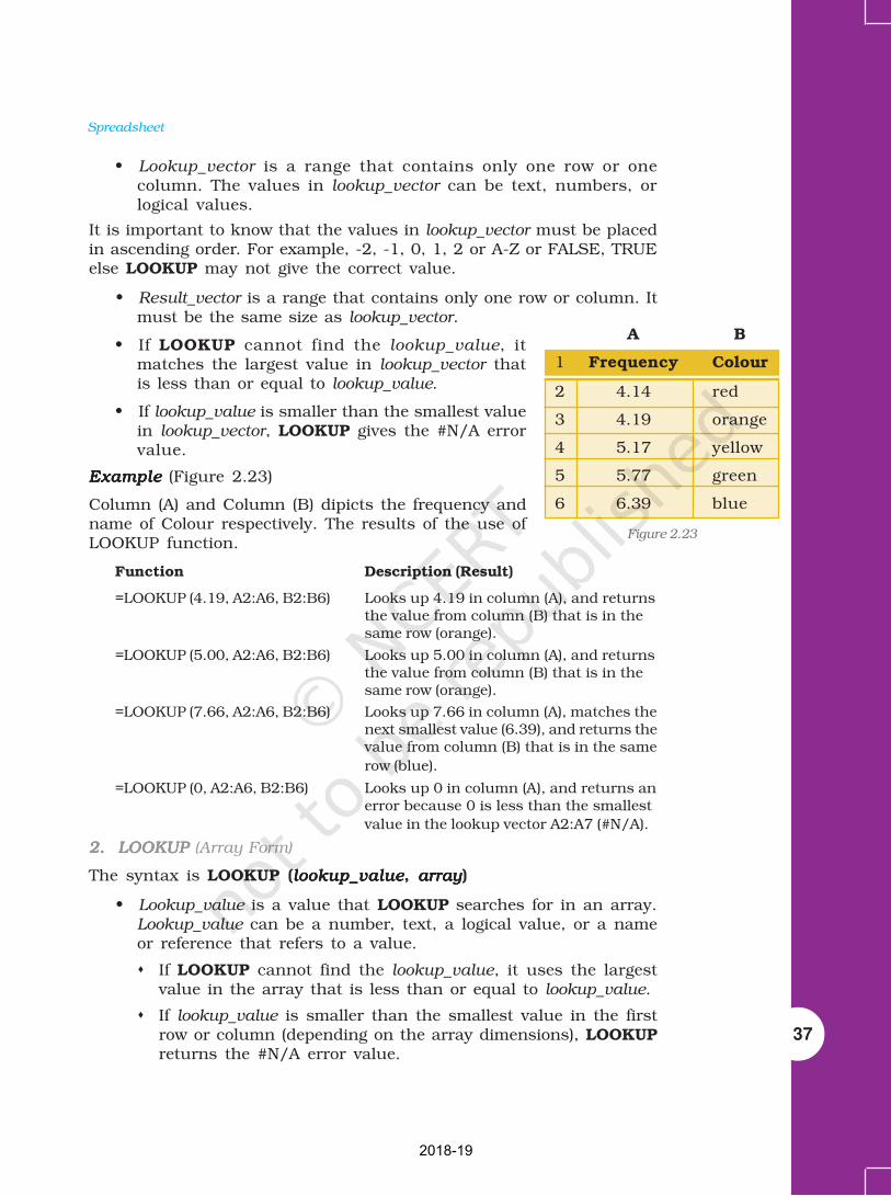
Spreadsheet
37
• Lookup_vector is a range that contains only one row or onecolumn. The values in lookup_vector can be text, numbers, orlogical values.
It is important to know that the values in lookup_vector must be placedin ascending order. For example, -2, -1, 0, 1, 2 or A-Z or FALSE, TRUEelse LOOKUP may not give the correct value.
• Result_vector is a range that contains only one row or column. Itmust be the same size as lookup_vector.
• If LOOKUP cannot find the lookup_value, itmatches the largest value in lookup_vector thatis less than or equal to lookup_value.
• If lookup_value is smaller than the smallest valuein lookup_vector, LOOKUP gives the #N/A errorvalue.
ExampleExampleExampleExampleExample (Figure 2.23)
Column (A) and Column (B) dipicts the frequency andname of Colour respectively. The results of the use ofLOOKUP function.
Function Description (Result)
=LOOKUP (4.19, A2:A6, B2:B6) Looks up 4.19 in column (A), and returnsthe value from column (B) that is in thesame row (orange).
=LOOKUP (5.00, A2:A6, B2:B6) Looks up 5.00 in column (A), and returnsthe value from column (B) that is in thesame row (orange).
=LOOKUP (7.66, A2:A6, B2:B6) Looks up 7.66 in column (A), matches thenext smallest value (6.39), and returns thevalue from column (B) that is in the same
row (blue).
=LOOKUP (0, A2:A6, B2:B6) Looks up 0 in column (A), and returns anerror because 0 is less than the smallestvalue in the lookup vector A2:A7 (#N/A).
2. LOOKUP2. LOOKUP2. LOOKUP2. LOOKUP2. LOOKUP (Array Form)
The syntax is LOOKUP (lookup_valuelookup_valuelookup_valuelookup_valuelookup_value, arrayarrayarrayarrayarray)
• Lookup_value is a value that LOOKUP searches for in an array.Lookup_value can be a number, text, a logical value, or a nameor reference that refers to a value.
If LOOKUP cannot find the lookup_value, it uses the largestvalue in the array that is less than or equal to lookup_value.
If lookup_value is smaller than the smallest value in the firstrow or column (depending on the array dimensions), LOOKUPreturns the #N/A error value.
A B
1 Frequency Colour
2 4.14 red
3 4.19 orange
4 5.17 yellow
5 5.77 green
6 6.39 blue
Figure 2.23
2018-19

38
Computerised Accounting System
• Array is a range of cells that contains text, numbers, or logicalvalues that we want to compare with lookup_value.
If array covers an area that is wider thanit is tall (more columns than rows),LOOKUP searches for lookup_value in thefirst row.
If array is square or is taller than it is thewide (more rows than columns), LOOKUPsearches in the first column.
Example Example Example Example Example (Figure 2.23(a))
Column (A) contains a, b, c, d some text values and Column (B)contain 10, 20, 30, and 40 some numbers. The Array is A1:B4.
The LOOKUP function used for different alpha character as follows:
Function Description (Result)
=LOOKUP (“c”, A1:B4) Looks up “C” in first row of the arrayand returns the value in the lastrow that is in the same column (30).
=LOOKUP (“b”, A1:B4) Looks up “b” in first row of the arrayand returns the value in the last column
that is in the same row (20).
3. VLOOKUP3. VLOOKUP3. VLOOKUP3. VLOOKUP3. VLOOKUP
The VLOOKUP function, which stands for vertical lookup, helps us tofind specific information in large data tables such as an inventory listof parts or a large employee contact list. The VLOOKUP functionsearches and matches first the required value from the column of arange of cells, and then returns a value from any cell on the same rowof the range. The syntax is
VLOOKUP (lookup_value, table_array, col_index_num, range_lookup)where
Lookup_value - The value to search in the first column of the table.Lookup_value can be a value or a reference. If lookup_value is smallerthan the smallest value in the first column of table_array, VLOOKUPreturns the #N/A error value.
Table_array - Two or more columns of data. Use a reference to arange or a range name. The values in the first column of table_arrayare the values searched by lookup_value. These values can be text,numbers, or logical values. Uppercase and lowercase texts areequivalent.
Col_index_num – The column number in table_array from which thematching value must be returned. A col_index_num of 1 returns thevalue in the first column in table_array; a col_index_num of 2 returns
A B
1 a 10
2 b 20
3 c 30
4 d 40
Figure 2.23(a)
2018-19

Spreadsheet
39
the value in the second column in table_array, and so on. Ifcol_index_num is:
• Less than 1, VLOOKUP returns the #VALUE! error value.
• Greater than the number of columns in table_array, VLOOKUPreturns the #REF! Error value.
Range_lookup – A logical value that specifies whether we wantVLOOKUP to find an exact match or an approximate match:
• If TRUE or omitted, an exact or approximate match is returned.If an exact match is not found, the next largest value that is lessthan lookup_value is returned. The values in the first column oftable_array must be placed in ascending sort order; otherwise,VLOOKUP may not give the correct value.
• If FALSE, VLOOKUP will only find an exact match. In this case,the values in the first column of table_array do not need to besorted. If there are two or more valuesin the first column of table_array thatmatch the lookup_value, the firstvalue found is used. If an exact matchis not found, the error value #N/A isreturned.
In the following examples we will explainthe steps how the VLOOKUP function tofind the specific information from thespreadsheet table.
Example -1Example -1Example -1Example -1Example -1 (Refer Figure 2.24) to find outemployee’s Basic Pay
=VLOOKUP (A3, A1:D7, 4, FALSE)
Lookup the Basic Pay for Employee Code3456 (A3) in the first column and returnthe matching value in the same row of thefourth column i.e. 3453.00(d3).
Example - 2Example - 2Example - 2Example - 2Example - 2 (Refer Figure 2.25)
In this example we search the column Item-ID of baby products from the table A2 :D6and match the values in the Cost (columnnumber 3) and Markup (column number 4) columns to calculate pricesand with different test conditions. The final result of the function isalso given after description.
Function Description
= VLOOKUP (“DI-328”, A2:D6, 3, Calculates the retail price of diapers byFALSE) * (1 + VLOOKUP (“DI-328”, adding the markup percentage to theA2:D6, 4, FALSE)). cost. Result Rs. 28.96
Figure 2.24
Figure 2.25
2018-19

40
Computerised Accounting System
= (VLOOKUP (“WI-989”, A2:D6, 3, Calculates the sale price of wipes byFALSE) * (1 + VLOOKUP (“WI-989”, subtracting a specified discount 4,A2:D6, FALSE))) * (1 - 20%). from the retail price Result .Rs. 5.73
= IF(VLOOKUP(A2, A2:D6, 3, If the cost of an item is greater thanFALSE) >= 20, “Markup is” and or equal to Rs. 20.00, displays the100 * VLOOKUP (A2, A2:D6, 4, string “Markup is nn%”; otherwise,FALSE) and ”%”, “Cost is under displays the string “Cost is underRs.20.00”). Rs. 20.00”.
Result: Markup is 30%
= IF (VLOOKUP (A3, A2:D6, 3, If the cost of an item is greater thanFALSE) >= 20, “Markup is:” and or equal toRs.20.00, displays the string100 * VLOOKUP (A3, A2:D6, 4, Markup is nn%”; otherwise, displaysFALSE) and”%”, “Cost is Rs.” and the string “Cost is Rs.n.nn”.VLOOKUP (A3, A2:D6, 3, FALSE)) Result: Cost is Rs. 3.56
4. HLOOKUP4. HLOOKUP4. HLOOKUP4. HLOOKUP4. HLOOKUP
The HLOOKUP function (short name of Horizontal Lookup), searchesfor a value in the first row of a table array and returns the correspondingvalue in the same column from another row of the same table array.The syntax for HLOOKUP is as follows:
HLOOKUP(lookup_value, table_array, row_index_num,range_lookup) where
• Lookup_value – The value to search for in the first row of thetable array.
• Table_array – Two or more rows of data. The values in thefirst row of the table_array are the values searched for thelookup_value. These values can be text, numbers, or logicalvalues. Uppercase and lowercase texts are equivalent.
• Row_index_num – The row number in table_array from whichthe corresponding value must be returned. A row_index_numof 2 returns the value in the second column in table_array; arow_index_num of 3 returns the value in the third column intable_array, and so on.
• Range_lookup – A logical value that specifies whether wewant HLOOKUP to find an exact match or an approximatematch. If set to “FALSE”, a corresponding value will be returnedonly if an exact match is found. If set to “TRUE”, the nearestmatch will be considered if an exact one is not found.
Let us take a simple example to understand the HLOOKUP function:In the following two different worksheets:
Example Example Example Example Example (Figure 2.26 and 2.27)
Worksheet 1 - The values for Budget are in Row 2 corresponding toeach Quarter in Row 1.
2018-19

Spreadsheet
41
Worksheet 2 - Corresponding to each Quarter(column (C)); some part of budget is Spent(column (E)) – which is listed vertically. Wewant to pick the budget for each quarter fromthe Worksheet 1 and put it in column (D) ofWorksheet 2 and then calculate the amountPending (column (F)) correspondingly. In cellD2:D5 we will enter the HLOOKUP functionas follows: (as shown for D4 cell) = HLOOKUP(C4; Budget! $A$1:$E$2; 2; FALSE) where inthis function.
C4 lookup value, for thequarter
budget!$B$1:$E$2 Table array, found in worksheet 1: namedbudget.
2 Row_index_num, is the row 2 in worksheet1: named Budget
FALSE We want to find an exact match
Pending = D4-E4 Copy both the functions fromD4 to the Cells D2, D3 and D5 and fromF4 to Cells F2, F3 and F5 can be copied.
It is important to note that whenever any table array (or array) isreferred in lookup functions the cell address referred (normally it isrelative) must be converted in to absolute cell addresses.
2.1.2.6 Financial Functions
1. ACCRINT1. ACCRINT1. ACCRINT1. ACCRINT1. ACCRINT
This function returns the accrued interest for a security that paysperiodic interest. The syntax of this is as follows:
ACCRINT (issue, first_interest, settlement, rate, par, frequency, basis,calc_method)
Dates should be entered by using the DATE function, or as resultsof other formulas or functions. For example, use DATE (2008, 5, 23) forthe 23rd day of May, 2008. Problems can be occur if dates are enteredas text.
Issue is the security’s issue date.
first_interest is the security’s first interest date.
Settlement is the security’s settlement date. The securitysettlement date is the date after the issue date whenthe security is traded to the buyer.
Rate is the security’s annual coupon rate.Par is the security’s par value. By default Par is 1000
Figures 2.26 and 2.27
2018-19

42
Computerised Accounting System
Frequency is the number of coupon payments per year.For annual payments, frequency = 1; for Semi-annual, frequency = 2; for quarterly, frequency = 4.
Basis is the type of day count basis to use.
Excel stores dates as sequential serial numbers so they can beused in calculations. By default, January 1, 1900 is serial number 1,and January 1, 2008 is serial number 39448 because it is 39,448 daysafter January 1, 1900; in Excel for the ACCRINT is calculated as follows:
1
1
NC
1
rate AACCRINT par
frequency NLλ
= × ×
2. CUMIPMT2. CUMIPMT2. CUMIPMT2. CUMIPMT2. CUMIPMT
This function returns the cumulative interest paid between two periods(Refer Figure 2.28). The syntax of the function is:
CUMIPMT (rate, nper, pv, start_period, end_period, type)
Rate is the interest rate.
Nper is the total number ofpayment periods.
Pv is the present value.
Start_period is the first period in thecalculation. Paymentperiods are numberedbeginning with 1.
End_period is the last period in thecalculation.
Type is the timing of the payment (which may be either 0 or 1)
0 (zero) means Payment at the end of the period
1 means Payment at the beginning of the period.
3. PV3. PV3. PV3. PV3. PV
This function returns the present valueof an investment. The present value isthe total amount that a series of futurepayments is worth now. For example,when we borrow money, the loan amountis the present value (Figure 2.29). Thesyntax of the function is :
PV (rate, nper, pmt, fv, type) where
Rate is the interest rate per period.For example, for an automobile loan at a
Figure 2.28
Figure 2.29
2018-19

Spreadsheet
43
10% annual interest rate and installments are made the monthlypayments, then the interest rate per month is 10%/12, or 0.83%. Thevalue for rate into the function will be 10%/12, or 0.83%, or 0.0083.
Nper is the total number of payment periods in an annuity. Forexample, if this loan is a four-year car loan and makes monthlypayments, then loan has 4*12 (or 48) periods. The value for nper willbe 48.
Pmt is the payment made each period and cannot be change overthe life of the annuity. Typically, pmt includes principal and interestbut no other fees or taxes. For example, the monthly payments on anRs.10, 000, for four-year car loan at 12 per cent are Rs. 263.33. Wehave to enter -263.33 into the function as the pmt. If pmt is omitted,then fv must be included in the argument.
Fv is the future value, or a cash balance to attain after the lastpayment is made. If fv is omitted, it is assumed to be 0 (the futurevalue of a loan, for example, is 0). For example, if we want to saveRs. 50,000 to pay for a special project in 18 years, then Rs. 50,000 isthe future value. Then it is necessary to guess an interest rate anddetermine how much to save each month. If fv is omitted, then pmt
must be included as the argument.
Type is the number 0 or 1 and indicates when payments are due.The fv and type arguments are optional. The fv argument is the futurevalue or cash balance that we want to have after making last payment.If we omit the fv argument, Excel assumes a future value of zero. Thetype argument indicates whether the payment is made at the beginningor end of the period: (0 or omit the type argument when the payment ismade at the end of the period and use 1 when it is made at the beginningof the period).
When using financial functions, keep in mind that the fv, pv, andpmt arguments can be positive or negative, depending on whether weare receiving the money or paying out the money. It may be noted thatif we want to express the rate argument in the same units as the nper
argument, so that if we make monthly payments on a loan and weexpress the nper as the total number of monthly payments, as in 360(30×12) for a 30-year mortgage, we need to express the annual interestrate in monthly terms as well. Excel solves for one financial argumentin terms of the others. If rate is not 0, then:
If rate is 0, then:
(pmt * nper) + pv + fv = 0
nper
nper
pv * (1 rate ) pmt(1 rate * type) *
(1 rate ) 1 fv C
rate
+ + +
+ −+ =
2018-19

44
Computerised Accounting System
An annuityannuityannuityannuityannuity is a series of constant cash payments made over acontinuous period. For example, a car loan or a mortgage is an annuity.
4. FV4. FV4. FV4. FV4. FV
This function returns the future value of an investment based onperiodic, constant payment and a constant interest rate (Figure 2.30).The syntax of the function is :
FV (rate, nper, pmt, pv, type) where
Rate is the interest rate per period.
Nper is the total number of payment periods in an annuity.
Pmt is the payment made each period; it cannot change overthe life of the annuity. Typically, pmt contains principaland interest but no other fees or taxes. If pmt is omitted,then include the pv value in the argument.
Pv is the present value, or the lump-sum amount that aseries of future payments is worth right now. If pv isomitted, it is assumed to be 0 (zero), and then includethe pmt value in the argument.
Type is the number 0 or 1 and indicates when payments aredue. If type is omitted, it is assumed to be 0.
ExampleExampleExampleExampleExample
Figure 2.30
In the function FV (rate, nper, pmt, pv, type); the values aresubstituted as given in different cells of the worksheets and the resultcell A8 is having Rs. 2581.40 first worksheet for type is 1 while insecond worksheet shows the value of result Rs. 2571.18 for type is 0.
2018-19

Spreadsheet
45
5. PMT5. PMT5. PMT5. PMT5. PMT
The PMT function calculates the periodic payment for an annuity,assuming equal payments and a constant rate of interest (Figure2.26(d)). The syntax of PMT function is as follows:
= PMT(rate, nper, pv, [fv], [type]) where
rate is the interest rate per period,
nper is the number of periods,
pv is the present value or the amount the future paymentsare worth presently,
fv is the future value or cash balance that after the lastpayment is made (a future value of zero when we omit thisoptional argument)
type is the value 0 for payments made at the end of the periodor the value 1 for payments made at the beginning of theperiod.
The PMT function is often used to calculate the payment for mortgageloans that have a fixed rate of interest.
ExampleExampleExampleExampleExample (Figure 2.31)
In the sample worksheet that contains atable using the PMT function to calculateloan payments for interest rate 8% perannum and principal amount Rs. 1000/-
Here we have used both values of type= 0 and 1
6. RATE6. RATE6. RATE6. RATE6. RATE
This function returns the interest rate per period of an annuity. RATEis calculated by iteration and can have zero or more solutions. If thesuccessive results of RATE do not converge to within 0.0000001 after20 iterations, RATE returns the #NUM! error value (2.32). The syntaxof the function is as follows:
RATE (nper, pmt, pv, fv, type, guess) where.
Nper is the total number of paymentperiods in an annuity.
Pmt is the payment made each periodand cannot change over the lifeof the annuity. Typically, pmtincludes principal and interestbut no other fees or taxes. If pmtis omitted, then include the fvas argument.
Figure 2.31
Figure 2.32
2018-19

46
Computerised Accounting System
Pv is the present value — the total amount that a series offuture payments is worth now.
Fv is the future value, or a cash balance attain after the lastpayment is made.
If fv is omitted, it is assumed to be 0 (the future value of aloan, for example, is 0).
Type is the number 0 or 1 and indicates when payments are due.
0 or omitted means payment is due at the end of the period 1means payment is due at the beginning of the period.
Guess is the guess for what the rate will be. If omitted, it is assumedto be 10 per-cent.
7. NPV7. NPV7. NPV7. NPV7. NPV
This function calculates the net present value of an investment byusing a discount rate and a series of future payments (negative values)and income (positive values). The syntax for the function is:
NPV (rate, value1, value2,…. ) where
Rate is the rate of discount over the length of oneperiod.
Value1, value2, ... are 1 to 254 arguments representing thepayments and income. Value1, value2, ... mustbe equally spaced in time and occur at the endof each period. NPV uses the order of value1,value2 …., to interpret the order of cash flows.It is essential that entry for payment and incomevalues are in the correct sequence.
The NPV investment begins one period before the date of the value1cash flow and ends with the last cash flow in the list. The NPVcalculation is based on future cash flows.
If n is the number of cash flows in the list ofvalues, the formula for NPV is:
NPV (Figure 2.33) is similar to the PVfunction (present value). The primarydifference between PV and NPV is thatPV allows cash flows to begin either atthe end or at the beginning of the period.Unlike the variable NPV cash flow values,PV cash flows must be constantthroughout the investment.
NPV is also related to the IRR function(internal rate of return). IRR is the rate forwhich NPV equals zero: NPV (IRR (...),) = 0.
ni
ii 1
values
(1 rate )−
=+
NPV
Figure 2.33
2018-19

Spreadsheet
47
2.2 DATA ENTRY, TEXT MANAGEMENT AND CELLFORMATTING
In any computerised business application, the basic requirement is toinput data; which may be either for processing parameters e.g. input ofdata parameters such as month number and name of the month or numberof working days, DA%, etc. for the processing of payroll of the companyor to update various data elements. In both the cases data should becorrect, accurate and should be in proper format. This means that datashould be validated, corrected and can be display in proper format.
By default in spreadsheet the numbers are right aligned and textsare left aligned. The spreadsheet can distinguish different types ofnumbers; recognise a date, a currency, or a percentage value or textetc. For example, if we type 16/04/1980 in a cell, spreadsheet willrecognise it as a date and act accordingly. The software processes thedata and generates the output; which should be in specific format.For example 1.5 might represent a value for one and half teaspoon inone spreadsheet while the same 1.5 would represent constant multiplierfor age in another spreadsheet etc.
2.2.1 DATA ENTRY
Excel also facilitates fast data entry; and automatically repeats dataor can fill data in different cells (column wise or row wise.) For example,if we repeatedly type the days of the week in different cells instead ofthat we could use the built-in data fill options to fill the differentcells with the days automatically. Some of the methods for data entryare mentioned below:
2.2.1.1 The data fill options
The Fill command can be used to fill data intoworksheet cells (Figure 2.36 & 2.37. The Excelprovides for entering data automatically tocontinue a series of numbers, number and textcombinations, dates, or time periods, based ona pattern that we require. However, to fillquickly in several types of data series, we selectcells and drag the fill handle ( A Fillhandle is the small black square in the lower-right corner of the selection. When we point tothe fill handle, the pointer changes to a blackcross (Refer Figure 2.34 and 2.35).
The fill handle is displayed by default, Click the MicrosoftOffice Button , and then click Excel Options.
1. Click Advanced, and then under Editing options, clear or selectthe Enable Fill handle and cell drag-and-drop check box to hide ordisplay the fill handle.
Figure 2.34
Figure 2.35
2018-19

48
Computerised Accounting System
2. To avoid replacing existing data when we drag the fill handle, tomake sure that the Alert before overwriting cells check box isselected. If we don’t want to receive a message about overwritingnon-blank cells, we can clear this check box.
After we drag the fill handle, the Auto Fill Options button appears
so that we can choose how the selection is filled. For example, we canchoose to fill just cell formats by clicking Fill Formatting Only, or wecan choose to fill just the contents of a cell by clicking Fill WithoutFormatting.
Option -1 Drag the fil l handle to fil l data into adjacent cellsOption -1 Drag the fil l handle to fil l data into adjacent cellsOption -1 Drag the fil l handle to fil l data into adjacent cellsOption -1 Drag the fil l handle to fil l data into adjacent cellsOption -1 Drag the fil l handle to fil l data into adjacent cells(Figure 2.38)
For example, we want to enterdata in A1:A10 starting valuefrom 10 and in step of 10 wewill get 10, 20, … 100 by usingdrag option as shown in theFigure 2.34 and Figure 2.35respectively.
1. Select the cells that contain the data that we want tofill (A1:A2) into adjacent cells (A3:A10).
2. Drag the fill handle across the cells that we want tofill.
3. To choose how we want to fill the selection, click Auto FillOptions, and then click the option that we want.
Figure 2.36
Option - 2 fill the active cell with the contents of an adjacent cellOption - 2 fill the active cell with the contents of an adjacent cellOption - 2 fill the active cell with the contents of an adjacent cellOption - 2 fill the active cell with the contents of an adjacent cellOption - 2 fill the active cell with the contents of an adjacent cell
1. Select an empty cell (A1) enter the value 10.
2. On the Home tab, in the Editing group, click Fill, and then clickon Series option.
Figure 2.38
Figure 2.37
2018-19

Spreadsheet
49
3. The option window provides direction (row wise i.e., B1:J1 or columnwise i.e., A2:A10) selection. The main option is Step Value (i.e.increment to the previous cell values in linear form) it is 10 in thisexample with respect to cell A1 and while another option is StopValue ( i.e. last value of the data when it is achieved the data fillstops) is 100 which may be in cell A10.
4. Once we enter the all the options and click OK, we get data filled inthe series A1:A0 as 10:100 in step of 10.
Observe the another example for Date data we can use fill handle(it is important to note that all the cells of the columns or rows shouldbe defined in (required) date data format using Format Cells). In thisexample we will enter date 24-11-1952 (or 24-Nov-1952) in cell A1 and24-12-1952 (or 24-Dec-1952) in cell A2 and then use Auto Fill Optionsbutton between cells A3:A10; find the changes?
2.2.1.2 Import/Copy Data from other sources
One more method for data entry for any application we can use thefollowing easiest method which will transfer data into required cellsby copying or importing to Excel worksheet. These data files may beeither in text files or non-text files format.
Text files can be directly read using a text editor such as Note padin MS Windows. These files often have extension .txt but can haveother extensions (such as .csv known as Comma Separated Valuestext file), easily read into Excel.
To import the data from a text file following steps are important forFigure 2.39.
1. Create data file using Notepad program of MS Windows (to getNotepad screen on desktop; click on Start button -> All Programs -> Accessories -> Notepad).
2. A comma-separated data values in one line of this text file is a rowin a spreadsheet and each entry, separated by a comma, is a columnentry for that row.
3. In the first line provides names forthe columns of the spreadsheet.
4. In the next line onward startentering the data separate bycomma as per the names given infirst line.
5. It may possible that every datamay not be of similar length buteach data (even a blank data)should be separated by comma asper the names of the column.
6. Open a new Excel worksheet from the Office Button.
Figure 2.39
2018-19

50
Computerised Accounting System
7. Select Data Tab on the Ribbon.
8. On Data tab; an option Get External Data having From Text option.
9. Click on “From Text” which will allow selecting a Notepad file (Figure2.40 & 2.41) saved as .cvm into Excel format directly and data willbe copied into respective columns and rows.
10. Each and every data from Notepad file can be saved as an Exceldata file This provides a lead that Excel worksheet consists of fourtypes of data in cells: labels, values, date and formulas and datavalidation.
Figure 2.41Figure 2.40
• Labels (text) are descriptive data such as names, months andusually include alphabetic characters. Excel aligns text to theleft side of the cell.
• Values (numbers) are generally raw numbers or dates.
Whole value: If the data is a whole value, such as 34 or 5763,Excel aligns the data to the right side of the cell.
Vale with a decimal: If the data is a decimal value, Excelaligns the data to the right side of the cell, including thedecimal point, with the exception of a trailing 0. For example,if we enter 246.75, then 246.75 displays; such as 246.70, willdisplay as 246.7. We can change the display appearance,column width, and alignment of data.
• Formulas are instructions for Excel to perform calculations.
• Date: If we enter a date, such 16/12, Dec 16, or 16 Dec, Excelautomatically returns 16-Dec in the cell, but the Formula bardisplays 16/12/2008. (The Date format is dependent to CountrySpecific Format selection).
2.2.2 DATA VALIDATION
Data validation is a feature to define restrictions on type of data enteredinto a cell. We can configure data validation rules for cells data thatwill not allow users to enter invalid data, There may be warningmessages when users tries to type wrong data in the cell. The messagesalso guide users to what input is expected for the cell, and instructionsto correct any errors.
2018-19

Spreadsheet
51
Data validation is invaluable because it is necessary that data mustbe accurate and consistent. The different methods for data validationare as follows:
• Create a Drop down List – By this option pre-defined items nameslist is referred and restrict the users to select accordingly – e.g. Inthe organisation for a business application we want to restrict the
Figure 2.42
users not to enter the names of departments other than Sales,Finance, R&D, Operation, HR and IT, etc.; for qualification of eachemployee not to enter other than MBA, PHD, CA, MCA, ARCHITECTand MBBS, etc., and the Sex Code should be either “Male” or“Female” for the employees. Following are the steps described howto use drop down list: A drop-down list can be prepared in threedifferent ways which can be used for data validation (Figure 2.42).
• Type a list of values separated by commas, i.e. using delimitedlist e.g. Male, Female
• Select the cells on the worksheetwhose values can be used directlytyped in a single row or singlecolumn
• Select the data in cells and createa Named Range to refer
Open a blank worksheet
Enter the column titles e.gEmployee Name (cell A1),Department (cell B1), Quali-fication (cell C1) and Sex Code(cell D1) in the first row and fourdifferent columns respectively(Figure 2.42). Figure 2.43
2018-19

52
Computerised Accounting System
Enter the Names of Employees in thecolumn (a) (cells A2:A10).
Prepare a list of department namessome where in the worksheet (sayG3:G9).
Define the Named range ( usingFormula Tab ->Define Name on theribbon) say DEPT .
Select the column (b) e.g. Department(data to be validated in whole column).Figure 2.44
In the Data Tab of the ribbon click Data Validation on DataTools opens three Data Validation Tabs (Figure 2.43). The firsttab is Setting Tab select List for drop down list option.
This option will display Validation Criteria and to provide validdata List in the Source where we have to type Name of theRange as =DEPT (Figure 2.44). The two more options also
required clicking here one Ignore Blank box then empty orblank values won’t be allowed and other is In-cell drop down.
To display an input message when a cell (e.g. B2 later B3:B10) isselected, click the second tab on data validation option, i.e. InputMessage Tab (Figure 2.45) and enter the desired text in the Title(e.g. DEPT_T) and provide an input short message for the user(e.g. SELECT/ENTER DEPARTMENT). Also tick the option todisplay this message when the cell is selected (Figure 2.46).
To set the response settings when invalid data is entered intothe cell click on the third tab of data validation option (Figure2.46) i.e. Error Alert Tab. This tab enables :
(a) To display the error alert after invalid data is entered inthe box.
(b) Enter message allows to type the desired message foruser and title for reference purpose.
Figure 2.46Figure 2.45
2018-19
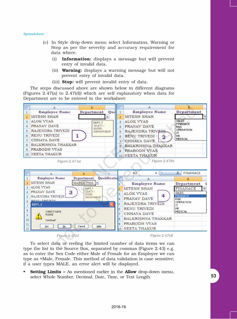
Spreadsheet
53
(c) In Style drop-down menu select Information, Warning orStop as per the severity and accuracy requirement fordata where.
(i) Information: displays a message but will prevententry of invalid data.
(ii) Warning: displays a warning message but will notprevent entry of invalid data.
(iii) Stop: will prevent invalid entry of data.
The steps discussed above are shown below in different diagrams(Figures 2.47(a) to 2.47(d)) which are self explanatory when data forDepartment are to be entered in the worksheet:
Figure 2.47 (a) Figure 2.47(b)
Figure 2.47(c) Figure 2.47(d)
To select data or reefing the limited number of data items we cantype the list in the Source Box, separated by commas (Figure 2.43) e.g.as to enter the Sex Code either Male of Female for an Employee we cantype as =Male, Female. This method of data validation is case sensitive;if a user types MALE, an error alert will be displayed.
• Setting Limits – As mentioned earlier in the Allow drop-down menu,select Whole Number, Decimal, Date, Time, or Text Length.
2018-19
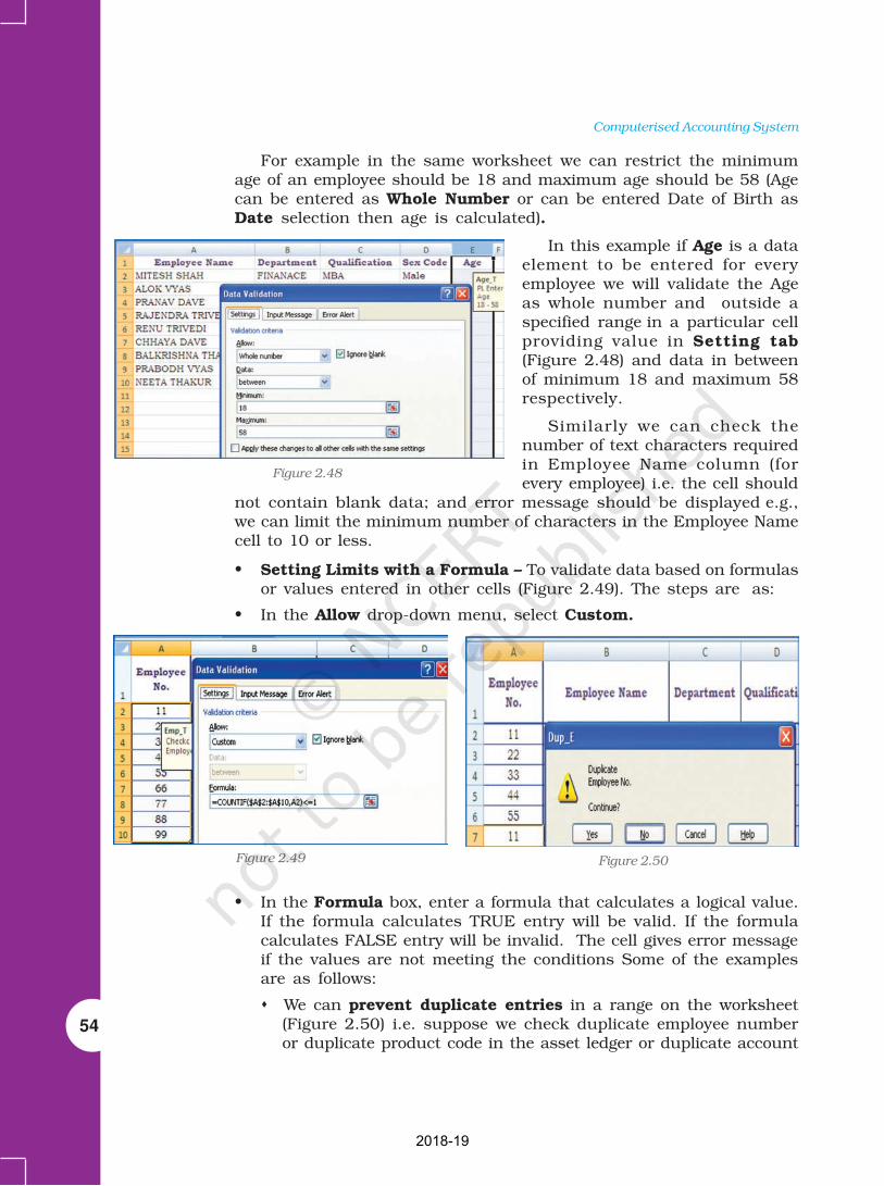
54
Computerised Accounting System
For example in the same worksheet we can restrict the minimumage of an employee should be 18 and maximum age should be 58 (Agecan be entered as Whole Number or can be entered Date of Birth asDate selection then age is calculated).
In this example if Age is a dataelement to be entered for everyemployee we will validate the Ageas whole number and outside aspecified range in a particular cellproviding value in Setting tab(Figure 2.48) and data in betweenof minimum 18 and maximum 58respectively.
Similarly we can check thenumber of text characters requiredin Employee Name column (forevery employee) i.e. the cell should
not contain blank data; and error message should be displayed e.g.,we can limit the minimum number of characters in the Employee Namecell to 10 or less.
• Setting Limits with a Formula – To validate data based on formulasor values entered in other cells (Figure 2.49). The steps are as:
• In the Allow drop-down menu, select Custom.
Figure 2.48
Figure 2.49 Figure 2.50
• In the Formula box, enter a formula that calculates a logical value.If the formula calculates TRUE entry will be valid. If the formulacalculates FALSE entry will be invalid. The cell gives error messageif the values are not meeting the conditions Some of the examplesare as follows:
We can prevent duplicate entries in a range on the worksheet(Figure 2.50) i.e. suppose we check duplicate employee numberor duplicate product code in the asset ledger or duplicate account
2018-19

Spreadsheet
55
code for the same item entered by userit shows the error.
We can limit the sum value for a rangewhich will cause error if sum of thevalues exceeds the given total, i.e.suppose the total amount of budget isfixed and sum of the distribution ofthe amount for different items in therange exceeds then it shows the error(Figure 2.50(a)
We can prevent user from addingspaces before or after the text in entry. The TRIM functionremoves spaces before and after the text. This formula checksthat the entry is equal to trimmed entry (Figure 2.50(b).
Figure 2.50(a)
We can prevent entry of dates that falls on (weekends orholidays) Saturday or Sunday (or any other day). The WEEKDAYfunction returns the number for the date entered in the cell. Ifthe value is 1(it is Sunday) and 7 (it is Saturday) then data entryis not allowed (Figure 2.50(c) and error message will be displayed.
2.2.3 DATA VALIDATION FORM
To input data into a spreadsheet, often we type the data into cellsdirectly. That’s where data validation comes in handy. Instead of typingthe same thing again and again, we can enter data into cells using
Figure 2.50(c)Figure 2.50(b)
A form, whether printed or online, is a document designed with astandard structure and format that makes it easier to capture, organise,and edit information. A data form is a dialog box that displays onecomplete record at a time. Data forms can be used to add, change,locate, and delete records.
2018-19

56
Computerised Accounting System
drop-down lists or using data input form. Using a data form can makedata entry easier than moving from column to column when we havemore columns of data than can be viewed on the screen. To createinput data form it is necessary that all the data names must be enteredin the first row of the worksheet, because the input form refers these
data names. To create input data form we have to select the tool
as Form button to the Quick Access Toolbar .
The Form button has not been included on the user interface Ribbon,but we can still use it in Excel 2007 by adding at Quick Access Toolbarusing following commands:
1. Click the arrow next to the QuickAccess Toolbar, and then click MoreCommands.
2. In the Choose commands from box,click All Commands.
3. In the list box, select the Formbutton, and then click Add.
The data form is useful, when data areof in a simple form of text boxes thatlist the column headings as labels issufficient and don’t requiredsophisticated or custom form features,such as a list box or spin button.
Excel automatically generates a built-in data form (Figure 2.51).The data form displays all column headers as labels in a single dialogbox. Each label has an adjacent blank text box in which we can enterdata for each column, up to a maximum of 32 columns. In a data form,we can enter new rows, find rows by navigating or (based on cellcontents) update rows and delete rows. If a cell contains a formula,the formula result is displayed in the data form, but we cannot changethe formula by using the data form.
2.3 DATA FORMATTING
Formatting of spreadsheets makes easier to read and understand heimportant information (e.g. conditional formatting, number formatting,text and general spreadsheet formatting etc.). On the Ribbon there areseveral tools and shortcuts to format spreadsheets effectively. Some ofthem are described as follows:
2.3.1 FORMATTING TOOLS
The formatting tools for:
• Number formatting – Number formatting includes adding per centsymbols (%), commas (,), decimal places, and currency signs ($,
Figure 2.51
2018-19

Spreadsheet
57
Rs. etc), date, time, scientific values and as well as some specialformats to a spreadsheet. The type of number format can bedetermined once the data is entered into the cell. Here are someexamples:
Currency: If we enter a financialvalue complete with the dollar/currency sign and two decimalplaces, Excel assigns a Currencyformat to the cell alongwith theentry.
Percentages: If we enter a valuerepresenting a percentage as a wholenumber followed by the per cent signwithout any decimal places, Excelassigns to the cell the percentageformat that follows this pattern along with the entry.
Dates: If we enter a date (dates are values, too) that follows oneof the built-in Excel number formats, such as 16-04-2009 or 16-Apr-2009 the program assigns a Date format that follows thepattern of the date.
Example – Explaining below the steps to format range B4:E7 ascurrency with zero decimal places using negative preset format.The sample unformatted worksheet is shown in the Figure 2.52(a)
Select the range to format, i.e.B4:E7
From the Ribbon select, HomeTab with Number option, clickon (Figure 2.52(b) to displayFormat Cells dialog box andchoose Number tab.
The Category list shows allthe preset formats availablein Excel, grouped intocategories. A samplecorresponding to the currentselection is shown at the topof the box.
Select the Category requiredi.e. Currency. The right handside of the box shows thedifferent symbols ofcurrencies. It also shows thepreset for negative valueseither minus sign (-) or red
Figure 2.52(a)
Figure 2.52(b)
2018-19

58
Computerised Accounting System
coloured number (if we do not want to display negative signdata).
Change the number of decimal places to Zero (0).
Click OK accept this format.
The output of these steps is shown in the Figure 2.52(c).
Similarly if we select the Category for the range H4:H8 asPercentage with Decimal Places to 2 digits. The Figure 2.52(d)will show the effect of this change.
Figure 2.52(c) Figure 2.52(d)
• Special Format Category
Special category data (special numbers)such as phone numbers, zip codes, andSocial Security numbers which requiredifferent format in a certain way (Figure2.52(e). From the Category option we selectSpecial and from corresponding drop-downbox under the Locale we select format specialnumbers appropriate to specific countries.
Figure 2.52(e)• Changing cell colours -
Select the range to format (e.g. B4:E7 –Figure 2.52(c).
From the Ribbon select Home Tab withNumber option, click on (Figure 2.42(b)to display Format Cells dialog box andchoose Fill tab.
Fill tab provide Background Colour,Pattern Colour and Pattern Style optionsfor the cell (or cell range to fill).
Select the colour required with desiredpattern style and pattern colour from theColour pallets (Figure 2.52(f).
Click OK and we see the result as givenin Figure 2.52(g).
Figure 2.52(f)
2018-19

Spreadsheet
59
There is other number a format tool onthe Ribbon for which allows number s toformat aesthetically such as :
In the Number section, click the CommaStyle button. Then the thousand digitnumbers or one hundred digit numbers will
be display with a commasign which makes iteasier to read. Excel alsoallows more precise with these numbers, that’s whyit added two decimal values.
To remove the decimal values, in the Numbersection of the Ribbon, click the Decrease Decimalbutton. That removes one decimal value. Click theDecrease Decimal button again to remove another
decimal value. Similarly we can use to Increase Decimal button twice.
To create own custom format, from theFormat Cell dialog box, click the Customcategory (Figure 2.52(h), select one of theexisting formats, and then proceed to createby adding appropriate or subtractingundesired characters.
We can find out the format used in a cellor some cells of unknown worksheet and canbe changed by using the Format Cells dialog.In this case Right-click the mouse buttonfor appropriate cell (s) or column (s) andchoose Format Cells. In the Category list,select one of the formats as percharacteristics from the right list or selectthe custom format.
Adding text formatting – The text formatting is mostly requiredfor presentation of final output and aesthetically reading of theinformation. There may be display of the text or numbers in differentFonts; Aligning in Cells,Changing Colour of Fonts,Merging of cell ranges toaccommodate data etc.(Figure 2.52(i & j)) When weinsert a Text box, it looksquite plain. We can formattext boxes to make themstand out on the worksheet;using the options from theRibbon; on Insert Tab with
Figure 2.52(g)
Figure 2.52 (i)
Figure 2.52 (j)
Figure 2.52(h)
2018-19

60
Computerised Accounting System
the Text dialog box. We can use these drawing tools in dressing themup with special formatting commands (Figure 2.52(j)). These tools allowus to add decorative and explanatory material to worksheet and chart.How the Illustrations Tools or Text Tools can be used; let usunderstand from the example using both the tools bars together.
• Change the font or font size in a worksheet (Figure 2.52(j)) andFigure 2.52(j)
1. Select the cell, range of cells, text, or characters that we want toformat.
2. On the Home tab, in the Font group, we will do the following:
To change the font, click the fontthat we want in the Font box.
To change the font size, click thefont size that we want in the FontSize box , or click Increase Font
Size or Decrease Font Size
until the size we want is displayed in the Font Size box.
• Change the cell border (Figure 2.52(k))
1. On a worksheet, select the cell or range of cells that we want to adda border to, change the border style on, or remove a border from.
2. On the Home tab, in the Font group, we will do one of thefollowing:
To apply a new or different border style, click the arrow next
to Borders , and then click a border style.
To remove cell borders, click the arrow next to Borders, and
then click No Border.
The Borders button displays the most recently used border style. We
can click the Borders button (not the arrow) to apply that style.
• Create a custom cell border (Figure 2.52(j) Figure 2.52(i)
We can create a cell style that includes a
custom border, and can apply to that cell style
when we want to display the custom border
around selected cells.
1. On the Home tab, in the Styles group,click Cell Styles.
2. Click New Cell Style.
3. In the Style name box, type an appropriate name for the newcell style.
4. Click Format.
Figure 2.52(k)
Figure 2.52(l)
2018-19

Spreadsheet
61
5. On the Border tab, under Line, in the Style box, click the linestyle that we want to use for the border.
6. In the Colour box, select the colour that we want to use.
7. Under Border, click the border buttons to create the borderthat we want to use.
8. Click OK.
9. In the Style dialog box, under Style Includes, clear the checkboxes for any formatting that we do not want to include in thecell style.
10. Click OK.
11. To apply the cell style, do the following:
12. Select the cells that we want to format with the custom cellborder.
13. On the Home tab, in the Styles group, click Cell Styles.
14. Click the cell style that we want to apply.
• Conditional Formatting
Conditional formatting helps us for specific questions about data. Wecan apply conditional formatting to a cell range, a table, or a PivotTablereport. There are important differences to understand when we useconditional formatting on a PivotTable report (Figure 2.52(k).
• The benefits of conditional formatting (Figure 2.52m)
To analyse data, we often ask ourselves some questions,such as:
Where are the exceptions in a summary of dataover the past five years?
What is the trend in data over the past two years?
Who is responsible for such results during thismonth?
What is the overall age distribution of employees?
Which products have greater than 10% revenueincreases from year to year?
Who are the highest performing and lowestperforming students in the class?
Conditional formatting helps to answer these questions by making iteasy to highlight interesting cells or ranges of cells, emphasise unusualvalues, and visualise data by using data bars, colour scales, and iconsets. A conditional format changes the appearance of a cell range basedon a condition (or criteria). If the condition is true, the cell range isformatted based on that condition; if the conditional is false, the cellrange is not formatted based on that condition.
Figure 2.52(m)
2018-19

62
Computerised Accounting System
• Format all cells by using a colour scale
Colour scales are visual guides that help us to understand datadistribution and their variation. A colour scale helps us to compare arange of cells by using a gradation of different colours. The shade ofthe colour represents higher or lower values. For example, in a greencolour are higher value cells and red colour for lower value cells.
If one or more cells in the range contain a formula that returns anerror, the conditional formatting is not applied to the entire range. Toensure that the conditional formatting is applied to the entire range, usean IS or IFERROR function to return a value other than an error value.
1. Select one or more cells in a range, table, orPivotTable report.
2. On the Home tab, in the Styles group, click thearrow next to Conditional Formatting, and thenclick Colour Scales. (Figure 2.52(n).
3. Select a two-colour scale.
• More than the two colours (Figure 2.52(o)
1. Select one or more cells in a range, table, orPivotTable report.
2. On the Home tab, in the Styles group, click thearrow next to Conditional Formatting, and thenclick Manage Rules. The Conditional FormattingRules Manager dialog box is displayed. Do one ofthe following:
To add a conditional format, click New Rule. The NewFormatting Rule dialog box is displayed.
To change a conditional format, do the following:
Figure 2.52(n)
Figure 2.52(o)
2018-19

Spreadsheet
63
1. Make sure that the appropriate worksheet, table, or PivotTablereport is selected in the Show formatting rules for list box.
2. Optionally, change the range of cells by clicking Collapse Dialogin the Applies to box to temporarily hide the dialog box, byselecting the new range of cells on the worksheet, and then byselecting Expand Dialog.
3. Select the rule, and then click Edit rule. The Edit FormattingRule dialog box is displayed.
4. Under Select a Rule Type, click Format all cells based ontheir values.
5. Under Edit the Rule Description, in the Format Style list box,select 3-Colour Scale.
6. To select a Minimum and Maximum Type do one of the following:
Format lowest and highest values Select Lowest Value andHighest Value. In this case, we do not enter a Minimum andMaximum Value.
Format a number, date, or time value Select Number, andthen enter a Minimum and Maximum Value.
Format a percentage Select Per cent, and then enter aMinimum and Maximum Value. Valid values are from 0 (zero)to 100. Do not enter a per cent sign. Use a percentage whenwe want to visualise all values proportionally because thedistribution of values is proportional.
Format a percentile Select Percentile and then enter aMinimum and Maximum Value. Valid percentiles are from 0(zero) to 100.
Percentile is usually used we want to visualise a group of highvalues (such as the 20th percentile) in one colour grade proportionbecause they represent extreme values that might skew the visualisationof the data.
Format a formula result Select Formula, and then enter aMinimum and Maximum Value.
The formula must return a number, date, or time value. Start theformula with an equal sign (=). It’s a good idea to test the formula in theworksheet to make sure that the formula doesn’t return an error value.
• Changing the alignment of data in cells (Figure 4.52(p)
There are several options to change the alignment of text (data) in cells
Text layoutText layoutText layoutText layoutText layout
Vertical alignment – To specify the vertical position of the text in ashape, select an option from the list (or from the tool box).
Text direction – To specify the orientation of the text in a shape, selectan option from the list.
2018-19

64
Computerised Accounting System
2. Autofit2. Autofit2. Autofit2. Autofit2. Autofit
Resize shape to fit text - To increase the size of the shape verticallyso that the text fits inside of it, click this button.
3. Inter3. Inter3. Inter3. Inter3. Internal marnal marnal marnal marnal margingingingingin
The internal margin is the distance between the text and the outerborder of a chart element. We can increase or decrease the amount ofthis space by using the following options.
Left – To specify the distance between the left border of the selectedchart element and the text, enter the margin number that we want inthe Left box.
Right – To specify the distance between the right border of the selectedchart element and the text, enter the margin number that we want inthe Right box.
Top – To specify the distance between the top border of the selectedchart element and the text, enter the margin number that we want inthe Top box.
Bottom – To specify the distance between the bottom border of theselected chart element and the text, enter the margin number that wewant in the Bottom box.
Columns – To specify the number of columns of text in a chart elementand the spacing between the columns, click this button.
The commands for this
Select the range.
Click on Home tab for Alignment optionswhich displays the dialog box and selectthe alignment tab (Figure 2.38(n)(1).
Select horizontal and vertical as alignmentrequired.
There are other options to display text atangular orientation or text to be controlwithin cell or to spread within the cell.
Click OK.
• Merging a range of Cells
Merged cells are a single cell that is created by combining two or moreselected cells. The cell reference for a merged cell is the upper-left cellin the original selected range. When two or more adjacent horizontalor vertical cells are merged, the cells become one large cell anddisplayed across multiple columns or rows. The contents of one appearin the centre of the merged cell.
Figure 2.52(p)
2018-19

Spreadsheet
65
1. Select two or more adjacent cells that we want to merge.
2. On the Home tab, in the Alignment group, click Merge andCentre. (Or button).
3. The cells will be merged in a row or column, and the cell contentswill be centered in the merged cell. To merge cells withoutcentering, click the arrow next to Merge and Centre, and thenclick Merge Across or Merge Cells. The cell address of mergecells will be the address of lower active cell.
4. To change the text alignment in the merged cell,select the cell; click any of the alignment buttonsin the Alignment group on the Home tab.
• Split a merged cell (Figure 2.52(q)
1. Select the merged cell.
2. When we select a merged cell, the Merge and Centre buttonalso appears selected in the Alignment group on the Home tab.
3. To split the merged cell, click Merge and Centre. The contentsof the merged cell will appear in the upper-left cell of the rangeof split cells.
• Formatting a Table
There are predefined table styles (or quick styles) that we can use toquickly format a table. If the pre-defined table styles don’t meet ourneeds, we can create and apply a custom table style.
The table formatting by choosing Quick Styles options for tableelements, such as header and total rows, first and last columns, andbanded rows and columns.
• To choose a table style to create a table (Figure 2.52(r))
1. On the worksheet, select a range of cells that we want to quicklyformat as a table.
Figure 2.52(r)
Figure 2.52(q)
2018-19

66
Computerised Accounting System
2. On the Home tab, in the Styles group, click Format as Table.
3. Under Light, Medium, or Dark, click the table style that wewant to use.
Apply a table style to an existing table
1. On the worksheet, select the table to which we want to apply atable style.
2. On the Design tab, in the Table Styles group, do one of thefollowing:
Click the More button, from the dropdown menu, click thetable style (Light, Medium or Dark) that we want to use.
• Using the NOW function to add the current date to thespreadsheet
NOW ( ) is the function returns the serial number of the current dateand time. If the cell format was General before the function was entered,the result is formatted as a date.
Excel stores dates as sequential serial numbers so they can be usedin calculations. By default, January 1, 1900 is serial number 1, andJanuary 1, 2008 is serial number 39448 because it is 39,448 days afterJanuary 1, 1900. Numbers to the right of the decimal point in the serialnumber represent the time; numbers to the left represent the date. Forexample, the serial number 0.5 represents the time 12:00 noon.
• Adding Headers and Footers to Excel Spreadsheet
In spreadsheet, headers and footers are lines of textthat are printed at the top (header) and bottom (footer)of each page in the spreadsheet. They containdescriptive text such as titles, dates, and/or pagenumbers and are used to add information to a printedspreadsheet.
The headers and footers options are available inPage Layout view (Figure 2.53(a). For other sheettypes, such as chart sheets or for embedded chartswe can work with headers and footers in the PageSetup dialog box.
Add or change the header or footer text for aworksheet in Page Layout view
1. Click the worksheet to which we want to add/change headers orfooters.
2. On the Insert tab, in the Text group, click Header and Footer.(refer Figure 2.53(b)) Or Do one of the following:
To add a header or footer, click the left, centre, or right header orfooter text box at the top or at the bottom of the worksheet page.
Figure 2.53(a)
2018-19

Spreadsheet
67
To change a header or footer, clickthe header or footer text box at thetop or at the bottom of the worksheetpage that contains header or footertext, and then select the text that wewant to change.
3. Type the text that we want.
• Use Format Painter
To copy quickly formatting from one cell or group of cells to anotherpart of the spreadsheet uses the format painter. This feature isvery useful when extending a spreadsheet and we need to formatthe newly added cells to match the original ones.
• Use of AutoFormat Option
To quickly apply a number of formatting features to a spreadsheetwe can use one of the 17 AutoFormat styles available (in Excel2007). These styles combine a number of formatting options thatwill instantly give our spreadsheet a professional look.
2.4 OUTPUT REPORTS
We can print entire or partial worksheets and workbooks,one at a time, or several at once. The MS Excel canprint just the Excel table or also it provides to:
(a) Print a partial or entire worksheet orworkbook.
(b) Print several worksheets at once.
(c) Print several workbooks at once.
(d) Print an Excel table.
(e) Print a workbook to a file.
(f) Print a graphic Charts and Pivot Tables.
We can also print a workbook to a file instead of toa printer. This is useful when we need to print theworkbook on a different type of printer from the one toanother printer. The printing option is available to printquickly or to preview the printout before printing, clickMicrosoft Office Button, click the arrow next to Print, and then clickQuick Print or Print Preview (Figure 2.54). To print worksheet ortable; basic preparation for printing is required and describe below:
2.4.1 DEFINING THE PRINT AREA
By default, Excel prints all data on the current worksheet but forspecific and formatted print we have to define print area from the PageSetup dialog box or the Print Area command from the Page Layoutoption of the Ribbon (Figure 2.55).
Figure 2.54
Figure 2.53(b)
2018-19

68
Computerised Accounting System
• The Print Area using Dialog Box Option
1. Select the Page Layout command tabon the Ribbon.
2. In the Page SetupPage SetupPage SetupPage SetupPage Setup group, click PageSetup. The Page SetupPage SetupPage SetupPage SetupPage Setup dialog boxappears.
3. Select the Sheet tab.
4. In the Print Area text box, type therange of cells you want to print or toselect the area –
a. Click Collapse Dialog
b. Select the desired range of cells
c. Click Restore Dialog
5. Click OK and the print area is defined.
• The Print Area using Print Area Option
Excel keeps the print area defined until itis cleared or replaced. To set the print area:
1. Select the range of cells to print (e.g. A1:H10 of Figure 2.55)
2. Select the Page Layout command tab
3. In the Page Setup Page Setup Page Setup Page Setup Page Setup group, click Print Area» select Set PrintArea. The print area is set.
4. OPTIONAL: To add more data to the print area
a. select a range of cells
b. In the Page Setup group, click Print Area» select Add to PrintArea; the selected cells are added to any previously selecteddata.
c. Repeat steps a and b as necessary.
• To clear the print area
1. In the Page Setup Page Setup Page Setup Page Setup Page Setup group, click Print Area» select Clear PrintArea
Printing Ranges of CellsPrinting Ranges of CellsPrinting Ranges of CellsPrinting Ranges of CellsPrinting Ranges of Cells
We can manually select ranges of cells for printing and also have theoption of selecting multiple non-contiguous ranges for printing.
• To select Print Range manually (using key board only)
1. Select the range of cells to be printedor
From the Name Box pull-down list, select the range name to beprinted.
Figure 2.55
2018-19

Spreadsheet
69
2. In the top left corner of the Excel window, click the Office Button»select PrintPrintPrintPrintPrint or Press [Ctrl] + [P] the Print dialog box appears.
3. In the Print what section, select Selection.Selection.Selection.Selection.Selection.
4. Click OK. The specified range of cells is printed.
• To select Print Multiple Ranges
Excel facilitates to print non-contiguous ranges. Selected rangeswill print on separate pages.
1. Select the first range to be printed.
2. Press [Ctrl] + select the second range to be printed .
3. For each additional range to be printed, repeat step 2.
4. In the top left corner of the Excel window, click the Office Button– select PrintPrintPrintPrintPrint OR Press [Ctrl] + [P]. The Print dialog box appears.
5. In the Print what section, select Selection.Selection.Selection.Selection.Selection.
6. Click Print. The specified range of cells is printed.
2.5 PREPARATION OF REPORTS USING PIVOT TABLE
A Pivot Table is way to present information in a report format. APivotTable report often provides enhanced layout, attractive andformatted report with improved readability. This report is preparedfrom the spreadsheet once we add the fields with appropriate level ofdetails, calculations and group the data as per required information.The Pivot Table uses a List Data Table (Database).
2.5.1 ONE-VARIABLE DATA TABLE
• C1 cell is an input cell. We will create one-variable data tablewhich calculates the increase in the budget corresponding toeach of the possible increase in costs.
• If the data table is column-oriented, type the formula (=A2*C1) inthe row (row number 4) above the first value (in cell B5) and onecell to the right (in cell C4) of the column of values (Figure 2.56).
A data tabledata tabledata tabledata tabledata table is a range of cells that shows the results of substituting different valuesin one or more formulas. There are two types of data table: One-variable and two-variable.
One-variable data tableOne-variable data tableOne-variable data tableOne-variable data tableOne-variable data table (Figure 2.56(a) Formula used in a one-variable data tablemust refer to an input cell. The input cell is a cell used by Excel in which each inputvalue from a data table is substituted (column-oriented, i.e. input cell down onecolumn or row-oriented, i.e. across one-row).
TTTTTwo-variable data tablewo-variable data tablewo-variable data tablewo-variable data tablewo-variable data table (Figure 2.56(b) use only one formula with two lists of inputvalues. The formula must refer two different input cells.
2018-19

70
Computerised Accounting System
• Enter a column of values from B5:B10.
• Select all cells in the range B4:C10(Fig 2.56(a).
• On the Data tab on the Ribbon, in the DataTools group, click What-if-Analysis, andthen click Data Table (Figure 2.56(b).
• In the Row input cell box no entry.
• In the Column input cell box, enter $C$1
• Click OK to generate table.
2.5.2 TWO-VARIABLE DATA TABLE (Figure 2.57)
This we will learn by one simplest examplegenerating a mathematical table in which twoinput cells uses B1 and C1 to generate a 15×15multiplication table by multiplying each other.
• In a cell B2 on the worksheet, enter the formula(= B1 *C1) that refers to the two input cells.
Figure 2.56 Figure 2.56(b)
Figure 2.56(a)
Figure 2.57 Figure 2.57 (a)
2018-19

Spreadsheet
71
• Type one list of input values in thesame column below the (or fill theseries from 1 to 15 in B3:B17).
• Type the second list in the same row( or fill the series from 1 to 15 inC3:Q3), to the right of the formula.
• Select the range of cells thatcontains the formula and both therow and column of values i.e.B2:Q17.
• On the Data tab on the Ribbon, inthe Data Tools group, click What-if-Analysis, and then click Data Table.
• In the Row input cell box enter $B$1.
• In the Column input cell box, enter$C$1.
• Click OK to generate table (Figure 2.57(a))
2.5.3 PIVOT TABLES
The Pivot Table feature allows us to create across tabulation summary of data in whichheading can subsequently moved to givedifferent views of the data. We will understandwith the help of following example.
Example: A spreadsheet (Figure 2.58)provides the data for consumption from D2:D37(in Metric Tons) of three different vegetablesnamely Carrot, Onions and Potatoes during thethree days of the week in four different metrocities. The quota of consumption is fixed byFood Department to supply of these vegetablesin the city. The spread sheet shows the ActualConsumption and Surplus (i.e. = actual –quota).
• Click the data from A1: E37
• On the Insert tab on the Ribbon, in theTables group, click Pivot Table, andthen click Pivot Table to start Pivot TableReport interactive options (Figure 2.58(a)as Create Pivot Report (Figure 2.58(b).
• Enter the data location
• Choose to place the Pivot table on an Existing worksheet (sayG19).
Figure 2.58(a)
Figure 2.58
Figure 2.58(b)
2018-19

72
Computerised Accounting System
• Click OK to display a blank Pivot table and filed list (Figure2.58(c) and Excel displays the Pivot Table Toolbar
1. Drag the Field Names (Fromlocation number 1) to therequire positions in the pivottable (location Number 6).
2. Report Filter “Day”
3. Column Label “Vegetable”
4. Row Label “City”
5. Values “Sum of Actual” andthe final result will bedisplayed (Figure 2.58(d).
6. In the above selections at RowLabel we give “City” and then“Vegetable”; while in columnLabel if we do not enter anyselection. The Pivot Report willbe as shown in Figure 2.58(e).
The Pivot Table tool bar (Figure 2.58(f) provides various flexibility towork on data.
Figure 2.58(c)
Figure 2.58(d) Figure 2.58(e)
Figure 2.58(f) : Pivot Table Toolbar
2018-19

Spreadsheet
73
Advantages of Pivot Table (Report)
A PivotTable report is an interactive way to quickly summarise largeamounts of data. Use a PivotTable report to analyse numerical data indepth and to answer unanticipated questions about data. A PivotTablereport designed for:
Querying large amounts of data in user-friendly ways. Sub totalingand aggregating numeric data, summarising data by categories andsubcategories, and creating custom calculations and formulas.
Expanding and collapsing levels of data to focus on results, andproviding from details to the summary of data for areas of interest.
Moving rows to column or columns to rows (or “pivoting”) to seedifferent summaries of the source data.
Filtering, sorting, grouping, and conditionally formatting the mostuseful and the interesting subset of data to enable us to focus onthe information that we want.
Presenting concise, attractive, and annotated online or printedreports.
The use of a PivotTable report is to analyse related totals, when wehave a long list of figures to sum and to compare several factsabout each figure.
2.6. COMMON ERRORS (MESSAGES) IN SPREADSHEET
4.1.1 MARK COMMON FORMULA ERRORS
1. Click the Microsoft Office Button, click Excel Options, and thenclick the Formulas category.
2. In the Error Checking section, select the Enable background errorchecking check box.
3. To change the colour of the triangle that marks where an erroroccurs, in the Indicate errors using the colour box, select a newcolour.
4. Select a cell with a triangle in the top-left corner of a cell.
5. Next to the cell, click the Error Checking button that appears, andthen click the option that we want. The commands are different foreach type of error, and the first entry describes the error. If we clickIgnore Error, the error is marked to be ignored for each consecutivecheck.
6. Repeat the two previous steps.
• Correct an error value
If a formula cannot properly evaluate a result, e Excel will display an errorvalue. Each error type has different causes, and different solutions. Someare discussed here to understand them properly before redo the operation
Figure 2.59
2018-19

74
Computerised Accounting System
• Correct a ##### error
This error occur when a column is not wide enough, or a negative dateor time is used.
Reason: The column is not wide enough to display the content
1. Select the column by clicking the column header.
2. On the Home tab, in the Cells group, click Format, and thenclick AutoFit Column Width. Alternatively also we can double-click the boundary to the right of the column heading.
3. Select the column.
4. On the Home tab, in the Cells group, click Format, click FormatCells, and then click the Alignment tab.
5. Select the Shrink to fit check box.
Apply a different number format
In some cases, we can change the cell’s number format tomake the number fit within the existing cell width. Forexample, we can decrease the number of decimal placesafter the decimal point.
• Correct a #DIV/0! Error
This error occurs when a number is divided by zero (0).
1. Optionally, click the cell that displays the error, click the buttonthat appears, and then click Show Calculation Steps if it is appears.
Reasons
a. Entering a formula that contains explicit division by zero (0) —for example, =5/0.
Dates and times are negative numbersDates and times are negative numbersDates and times are negative numbersDates and times are negative numbersDates and times are negative numbers
When a date or time is typed in a cell, it appears in a default date and time format.The default date and time format is based on the Regional date and time settings thatare specified in Windows Control Panel, and changes when changes are made tothose settings. We can display numbers in several other dates and time formats, mostof which are not affected by Control Panel settings.
If we are using the 1900 date system, dates and times in Excel must be positivevalues.
When we subtract dates and times, make sure that we build the formula correctly.
If the formula is correct but the result is still a negative value, we can display thevalue by formatting the cell with a format that is not a date or time format.
1. On the HomeHomeHomeHomeHome tab, in the CellsCellsCellsCellsCells group, click ForForForForFormatmatmatmatmat, click ForForForForFormat Cellsmat Cellsmat Cellsmat Cellsmat Cells, andthen click the NumberNumberNumberNumberNumber tab.
2. Select a format that is not a date or time format.
Figure 2.60
2018-19

Spreadsheet
75
b. Using the cell reference to a blank cell or to a cell that containszero as a divisor.
Solutions
Change the cell reference to another cell.
Enter a value other than zero in the cell used as a divisor.
Enter the value #N/A into the cell referenced as the divisor,which changes the result of the formula to #N/A from #DIV/0!To denote that the divisor value is not available.
Prevent the error value from displaying by using the IF worksheetfunction. For example, if the formula that creates the error is=A5/B5, use =IF (B5=0,””, A5/B5) instead. The two quotationmarks represent an empty text string.
• Correct a #N/A error
This error occurs when a value is not available to a function or formula.
1. Optionally, click the cell that displays the error, click the button
that appears, and then click Show Calculation Steps if it appears.
Reasons and Solutions
a. Missing data, and #N/A or NA() has been entered in its place.
b. Giving an inappropriate value for lookup function as an argumentsuch functions may be HLOOKUP, VLOOKUP, MATCH or LOOKUP.
c. Using these lookup functions to locate the value in an unsortedtable.
d. Using an argument in the array formula that is not in the samenumber of rows or columns as the range that contains the arrayformula.
• Correct a #NAME? Error
This error occurs when Excel doesn’t recognize text in a formula.
Reasons:
a. The EUROCONVERT function without the Euro Currency Toolsadd-in being loaded.
Solutions1. Click the Microsoft Office Button , click Excel Options, and
then click the Add-ins category.
2. Select Excel Add-ins in the Manage list box, and then click Go.
3. In the Add-Ins available list, select the Euro Currency Toolscheck box, and then click OK.
• Correct #NULL! Error
This error occurs when we specify an intersection of two areas that donot intersect. The intersection operator is a space between references.
2018-19

76
Computerised Accounting System
1. Optionally, click the cell that displays the error, click the buttonthat appears, and then click Show Calculation Steps if it appears.
2. Possible causes and solutions.
Incorrect range operator
To refer to a contiguous range of cells, use a colon (:) to separatethe reference to the first cell in the range from the reference tothe last cell in the range. For example, SUM (A1:A10) refers tothe range from cell A1 to cell A10 inclusive.
To refer to two areas that don’t intersect, use the union operator,the comma (,). For example, if the formula sums two rangesmake sure that a comma separates the two ranges (SUM (A1:A10,C1:C10)).
Ranges do not intersect
If there are no squares at each corner of the colour-coded border,then the reference is to a named range.
If there are squares at each corner of the colour-coded border,then the reference is not to a named range.
5. Double-click the cell that contains the formula we want to change.Excel highlights each cell or range of cells with a different colour.
6. Do one of the following:
To move a cell or range reference to a different cell or range,drag the colour-coded border of the cell or range to the new cellor range.
To include more or fewer cells in a reference, drag a corner ofthe border.
In the formula, select the reference, and type a new one.
7. Press ENTER.
8. Do one of the following:
Select the range of cells that contains formulas in which wewant to replace references with names.
Select a single cell to change the references to names in allformulas on the worksheet.
9. On the Formulas tab, in the Defined Names group, click thearrow next to Define Name, and then click Apply Names.
10.In the Apply Names box, click one or more names.
• Correct#NUM! Error
This error occurs with invalid numeric values in a formula or function.
1. Optionally, click the cell that displays the error, click the buttonthat appears, and then click Show Calculation Steps if it appears.
2. Review the following possible causes and solutions:
2018-19

Spreadsheet
77
Using an unacceptable argument in a function that requires anumeric argument.
Make sure that the arguments (argument: The values that afunction uses to perform operations or calculations. The type ofargument a function uses is specific to the function. Commonarguments that are used within functions include numbers, text,cell references, and names.) used in the function are numbers.For example, even if the value we want to enter is $1,000, enter1000 in the formula.
Using a worksheet function that iterates, such as IRR or RATE,and the function cannot find a result.
Use a different starting value for the worksheet function.
Change the number of times Microsoft Office Excel iteratesformulas.
1. Click the Microsoft Office Button , click Excel Options, and
then click the Formulas category.
2. In the Calculation options section, select the Enable iterativecalculations check box.
3. To set the maximum number of times that Excel will recalculate,type the number of iterations in the Maximum Iterations box.The higher the number of iterations, the more time that Excelneeds to calculate a worksheet.
4. To set the maximum amount of change that we will accept betweencalculation results, type the amount in the Maximum Changebox. The smaller the number, the more accurate the result andthe more time that Excel needs to calculate a worksheet. Enteringa formula that produces a number that is too large or too smallto be represented in Excel.
• Correct a #REF! Error
This error occurs when a cell reference (cell reference: The set ofcoordinates that a cell occupies on a worksheet. For example, thereference of the cell that appears at the intersection of column B androw 3 is B3.) is not valid.
1. Optionally, click the cell that displays the error, click the buttonthat appears, and then click Show Calculation Steps if it appears.
2. Review the following possible causes and solutions:
Deleting cells referred to by other formulas, or pasting movedcells over cells referred to by other formulas.
Change the formulas, or restore the cells on the worksheet byclicking Undo immediately after we delete or paste the cells.
Using an Object Linking and Embedding (OLE) link to a programthat is not running.
Start the program.
2018-19

78
Computerised Accounting System
Linking to a Dynamic Data Exchange (DDE) topic such as “system”that is not available.
Make sure that we’re using the correct DDE topic.
Running a macro that enters a function that returns #REF!
• Correct a #VALUE! Error
This error occurs when the wrong type of argument (argument: Thevalues that a function uses to perform operations or calculations. Thetype of argument a function uses is specific to the function. Commonarguments that are used within functions include numbers, text, cellreferences, and names.) or operand (operand: Items on either side ofan operator in a formula. In Excel, operands can be values, cellreferences, names, labels, and functions.) is used.
1. Optionally, click the cell that displays the error, click the buttonthat appears, and then click Show Calculation Steps if it appears.
2. Review the following possible causes and solutions.
Entering text when the formula requires a number or a logicalvalue, such as TRUE or FALSE.
Microsoft Office Excel cannot translate the text into the correctdata type. Make sure that the formula or function is correct forthe required operand or argument, and that the cells that arereferenced by the formula contain valid values. For example, ifcell A5 contains a number and cell A6 contains the text “Notavailable”, the formula =A5+A6 will return the error #VALUE!.
Entering or editing an array formula, and then pressing ENTER.
Select the cell or range of cells that contains the arrayformula (array formula: A formula that performs multiplecalculations on one or more sets of values, and then returnseither a single result or multiple results. Array formulas areenclosed between braces { } and are entered by pressingCTRL+SHIFT+ENTER.), press F2 to edit the formula, and thenpress CTRL+SHIFT+ENTER.
Entering a cell reference, a formula, or a function as an arrayconstant.
Make sure that the array constant (constant: A value that is notcalculated and, therefore, does not change. For example, thenumber 210, and the text “Quarterly Earnings” are constants.An expression, or a value resulting from an expression, is not aconstant.) is not a cell reference, formula, or function.
Supplying a range to an operator or a function that requires asingle value, not a range.
Change the range to a single value.
Change the range to include either the same row or the samecolumn that contains the formula.
2018-19

Spreadsheet
79
SummarySummarySummarySummarySummary
• Setting up a spreadsheet can be fairly time consuming, although templates,or sample spreadsheets, are available with most of software packages. Thecomputeried spreadsheet can be formatted with different print layouts. Itallows working with rows and columns of numbers and use formula to do“what if” calculations. The spreadsheet gives considerable power andflexibility in entering and editing information, setting up calculations withformula and functions, and printing the results. It has rows that arehorizontal lines of information that are numbered on the left-hand side ofthe Excel workbook. Columns are vertical lines of information and areidentified by letters along the top of the spreadsheet. Rows and columnsintersect to form cells. A cell is addressed by the column and row position,for example B4 is the intersection of column b and row 4.
• In the earliest spreadsheets, cells were a simple two-dimensional grid.Over time, the model has been expanded to include a third dimension, andin some cases a series of named grids, called sheets.
• In any worksheet or spreadsheet a cell is the smallest element which maycontain a value or a formula or a function or it may simply be left empty. Touse formula or function in the cell; usually begin with = sign by convention.
• A cell reference is the name cell in the spreadsheet. Most cell referencesindicate another cell in the same spreadsheet, but a cell reference can alsorefer to a cell in a different sheet within the same spreadsheet or to a valuefrom a remote application. A typical cell reference consists the columnfollowed by a row number is called relative cell reference. Both columnand row number; either part can be relative changes when the cell orformula in it is moved or copied from other cell or absolute (indicated with$ in front of the part concerned of the cell reference). The older “R1C1”reference style consists of the letter R, the row number, the letter C, andthe column number; relative row or column numbers are indicated byenclosing the number in square brackets. Most current spreadsheets usethe A1 style, some providing the R1C1 style as a compatibility option. Whenthe computer calculates a formula in one cell to update the displayed valueof that cell, cell reference(s) in that cell, naming some other cell(s), causethe computer to fetch the value of the named cell(s).
• A reference to a range of cells is typically of the form (A1:A6) which specifiesall the cells in the range A1 through to A6. A formula such as “=SUM(A1:A6)” would add all the cells specified and put the result in the cellcontaining the formula itself.
• A function is a special key word which can be entered into a cell in order toperform and process the data which is appended within brackets. There isa function button on the formula toolbar (fffffx); which function offers assistance
2018-19

80
Computerised Accounting System
and useful prompts into a spreadsheet cell. Alternatively we can enter thefunction directly into the formula bar. A function involves four main issues:
• Name of the function.
• The purpose of the function.
• The function needs what argument(s) in order to carry its assignment.
• The result of the function.
• Formatting of spreadsheets makes easier to read and understand theimportant information (e.g. conditional formatting, number formatting, textand general spreadsheet formatting etc.). A cell or range can optionally bedefined to specify how the value is displayed. The default display format isusually set by its initial content if not specifically previously set, so that forexample “24/11/1952” or “24 Nov 1952” would default to the cell format of“date”. Similarly adding a % sign after a numeric value would tag the cellas a percentage cell format. The cell contents are not changed by thisformat, only the displayed value.
• To print an entire spreadsheet choose Page Setup from the File Menu,Choose the appropriate options in terms of horizontal (landscape) or vertical(portrait) printing, Excel prints entire spreadsheet document, if the documentis too wide to fit on a page, Excel will print the remaining columns onsubsequent pages before continuing to print the remaining rows.
• We can save our document every 5 minutes. The first time we save, go tothe File Menu and pull to Save, make sure the document is in the correctfolder and on the correct drive, type the name for what we want to save itas, and click in the save box.
2018-19

Spreadsheet
81
EXERCISE
Q1. MULTIPLE CHOICE QUESTIONS
1. The best way to get started in Excel 2007 is to click the _____.
a. View toolbar.
b. Home tab.
c. Microsoft Office Button.
d. None of the above.
2. Which key combination collapses the ribbon?
a. [Ctrl]+[F1]
b. [Ctrl]+[F3]
c. [Ctrl]+[F5]
d. [Ctrl]+[F7]
3. Which view shows margins and the rulers?
a. Normal
b. Page Layout
c. Page Setup
d. Review
4. As you type a number in a cell, what mode appears in the status bar?
a. Enter mode
b. Ready mode
c. Edit mode
d. Record mode
5. Where is the address of the active cell displayed?
a. Row heading
b. Status bar
c. Name Box
d. Formula bar
6. Which command reverses the last action performed in the worksheet?
a. Cut
b. Undo
2018-19

82
Computerised Accounting System
c. Redo
d. Paste
7. When navigating in a workbook, which command is used to move to thebeginning of the current row?
a. [Ctrl]+[Home]
b. [Page Up]
c. [Home]
d. [Ctrl]+[Backspace]
8. Which key when pressed displays the access keys?
a. [Alt]
b. [Ctrl]
c. [Shift]
d. [Esc]
9. Which command allows you to reverse an Undo command?
a. Redo
b. Repeat
c. Reset
d. Reverse
10. Which function results can be displayed in AutoCalculate?
a. SUM and AVERAGE
b. MAX and LOOK
c. LABEL and AVERAGE
d. MIN and BLANK
11. Which cell alignment is assigned to most values by default?
a. Right
b. Left
c. Centre
d. Decimal
12. Which function automatically totals a column or row of values?
a. TOTAL
b. ADD
c. SUM
d. AVG
2018-19

Spreadsheet
83
13. Which mathematical operator is represented by an asterisk (*)?
a. Exponentiation
b. Addition
c. Subtraction
d. Multiplication
14. Which step completes an entry and moves the pointer to the cell to the right?
a. Pressing [Enter]
b. Pressing [Tab]
c. Pressing [Shift]+[Tab]
d. Pressing [Shift]+[Enter]
15. How many blank worksheets are shown when a new workbook is created?
a. One
b. Two
c. Three
d. Four
Q2. ANSWER THE FOLLOWINGS QUESTIONS
1. Define spreadsheet and its salient features?
2. Write any five advantages using electronic spreadsheet in place of manualspreadsheet.
3. Define workbook and worksheet. What is the difference between them?
4. Explain active worksheet?
5. Using Fill: Series command in Excel write down the steps to fill data from120,320…..2300 in Column A.
6. Define Data Range, Name Range and How these are created and selected?
7. Write down the steps for the use of Custom Lists.
8. Explain the purpose of Format, Conditional Formatting and Auto Format.
9. What is Wrap Text feature of Excel, Merging of Cells and what will be the celladdress of merged cells?
10. Explain the purpose of using Print Preview?
11. Explain difference between relative reference and absolute reference?
12. Discuss IF function and nested IF functions giving example?
13. Write down examples for any two financial functions you know with their propersyntax.
2018-19
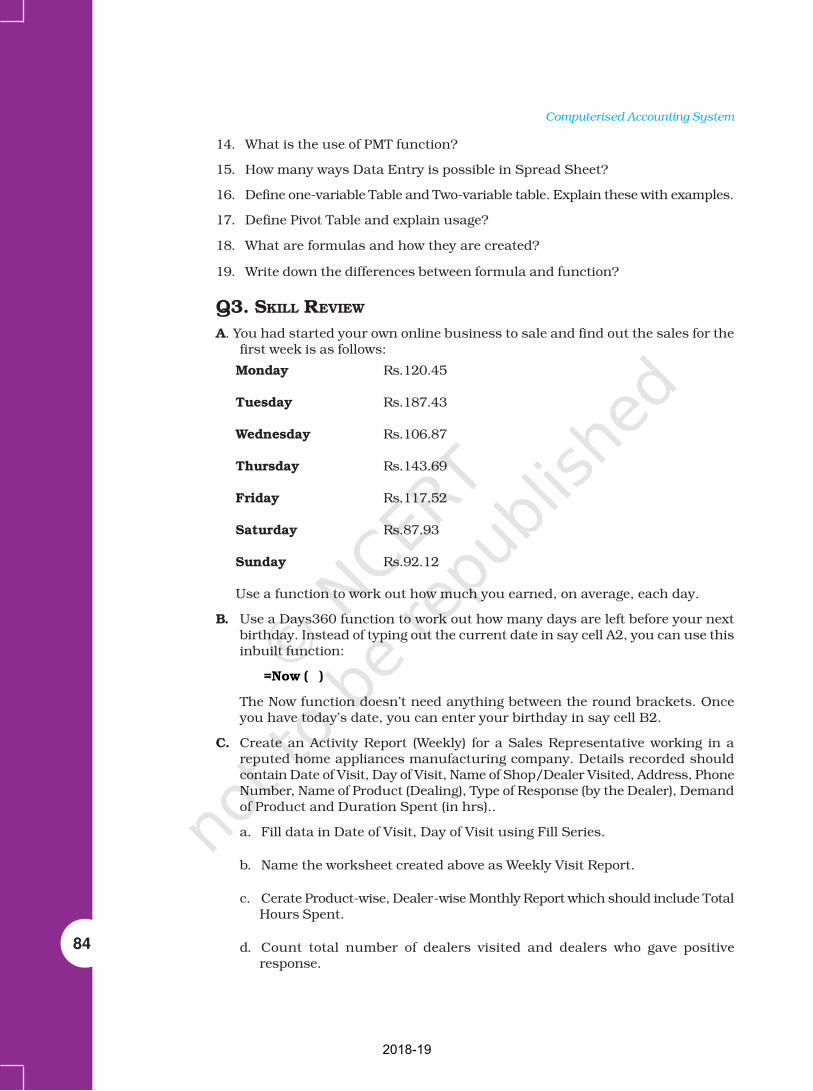
84
Computerised Accounting System
14. What is the use of PMT function?
15. How many ways Data Entry is possible in Spread Sheet?
16. Define one-variable Table and Two-variable table. Explain these with examples.
17. Define Pivot Table and explain usage?
18. What are formulas and how they are created?
19. Write down the differences between formula and function?
Q3. SKILL REVIEW
A. You had started your own online business to sale and find out the sales for thefirst week is as follows:
Monday Rs.120.45
Tuesday Rs.187.43
Wednesday Rs.106.87
Thursday Rs.143.69
Friday Rs.117.52
Saturday Rs.87.93
Sunday Rs.92.12
Use a function to work out how much you earned, on average, each day.
B. Use a Days360 function to work out how many days are left before your nextbirthday. Instead of typing out the current date in say cell A2, you can use thisinbuilt function:
=Now ( )
The Now function doesn’t need anything between the round brackets. Onceyou have today’s date, you can enter your birthday in say cell B2.
C. Create an Activity Report (Weekly) for a Sales Representative working in areputed home appliances manufacturing company. Details recorded shouldcontain Date of Visit, Day of Visit, Name of Shop/Dealer Visited, Address, PhoneNumber, Name of Product (Dealing), Type of Response (by the Dealer), Demandof Product and Duration Spent (in hrs)..
a. Fill data in Date of Visit, Day of Visit using Fill Series.
b. Name the worksheet created above as Weekly Visit Report.
c. Cerate Product-wise, Dealer-wise Monthly Report which should include TotalHours Spent.
d. Count total number of dealers visited and dealers who gave positiveresponse.
2018-19

Spreadsheet
85
Create a worksheet to record sales of home appliances sold by M/s Home MakerLtd. In the following format:
Date of Name of Name of Make Quantity SalesSales Customers Products Amount
The product lists includes Television sets, Refrigerators, Micro wave ovens,Water Coolers, Air Coolers, Geezers and Air conditioners of different Makes(and models). The cost of price of television is ranging from Rs. 10,000 toRs. 56,000; refrigerator is Rs. 13,000 to Rs. 45,000, micro wave ovens, watercoolers, geezers and air coolers are from Rs. 8,000 to Rs. 25,000 and AirConditioners are from Rs. 18,000 to Rs. 55,000. The shopkeeper sales theseproducts adding 17.25% more on cost price. He provides a discount of 4.35%on total amount if any customer purchases two products on the same date.Enter 30 records of different dates (for a month) and different customersaccordingly. Calculate the following:
a. Product wise weekly sales and discount.
b. Calculate the profit of shopkeeper.
c. Product wise total sales of the month and discount offered.
D. Create a worksheet to keep track of revenue collected and expenses done inconducting tour programs at different tourist places during 2004 to 2008.Format the numeric data in currency format, prepare year wise columns forrevenue and expenses for each tourist place and calculate the difference. Thecalculated difference may be negative, the format of negative balance may bered coloured. Use conditional formatting for higher and lower values of revenueand expenses. Align entire text in centre. The font of tourist place is Arial with14 point while the font of year is Times Roman with 14 points.
(Amount in lacs)
Tourist 2004 2005 2006 2007 2008 Place
Rev Exp Rev Exp Rev Exp Rev Exp Rev Exp
Manali 123 55 234 123 345 333 333 365 365 453
Kashmir 234 123 123 55 365 453 345 333 333 365
Shilong 345 333 333 365 123 55 234 123 456 233
Kerala 333 365 365 453 234 123 123 55 345 333
2018-19

86
Computerised Accounting System
ANSWERS
1. c 2. a 3. b 4. a 5. c 6. b
7. c 8. a 9. a 10. a 11. b 12. c
13. d 14. b 15. c
2018-19

Use of Spreadsheet in Business Application
87
USE OF SPREADSHEET
IN BUSINESS
APPLICATIONS
IntroductionAfter studying this chapter you will beable to use spreadsheet for:
• Computing employee’s grosssalary. Making necessarydeductions to calculate netsalary, payroll accounting.
• Calculation of deprecation byvarious methods.
• Loan repayment, interestcalculation.
3
In the previous chapter, we have learned aboutthe spreadsheet and its several features that canbe used in business applications. In this chapter,we shall discuss the applications of spreadsheet(using Excel) to Payroll Accounting and some otherselect applications (Asset Management, and LoanRepayment).
3.1 PAYROLL ACCOUNTINGEvery employee is paid salary on a pre-determineddate within the framework of employee contractand related personnel policy in force from time totime in an organisation.
The computation of salary payment is basedon the number of days an employee has worked,rate per grade of pay, rate of applied allowancesand deductions to be made therefrom.
The preparation of salary bill should providefor the following :
• Maintaining payroll related data such asEmployee No., Name, Attendance, Basic Pay,applicable Dearness and other Allowances,deductions to be made.
• Periodic payroll computations: the payrollcomputation includes the calculation of variousearning and deduction heads, which are to bederived from basic values (such as basic salary,number of days under leave without pay (LWP)and unauthorised absence, etc) as per theformulae.
2018-19

88
Computerised Accounting System
• Preparation of salary statement and employees salary slips
• Generation of advice to bank: It contains the net salary to betransferred to individual bank account of employees and other salaryrelated statutory payments such as provident fund, tax, etc.
3.1.1 PAYROLL COMPONENTS
Every employee is under contractual relationship of service with anorganisation, and is paid salary accordingly. The following elementsare important for salary computation and its payment:
• CURRENT PAYROLL PERIOD (MONTH AND YEAR)
• EARNINGS
Basic Pay (BP) : It is the pay in the pay scale plus Grade Pay,but does not include Special Pay.
Grade Pay (GP) : It is the pay to be added to the Basic Payaccording to the Designation of the employee and applicable payband or scale of pay.
Dearness Pay (DP) : It is that portion of Dearness Allowance,which has been declared and deemed to have been merged withthe Basic Pay.
Dearness Allowance (DA) : It is a compensation for erosion inthe purchasing power of wage earner due to price rise. It is grantedby the Government periodically as a percentage of (Basic Pay +Dearness Pay, if applicable).
House Rent Allowance (HRA) : It is an amount paid to facilitateemployee in acquiring on lease of residential accommodation.
Transport Allowance (TRA) : It is an amount to facilitate commutingto the the place of work, i.e. Delhi, Bhopal, Haridwar, etc.
Any Other Earning : It may include any other allowance notincluded above but declared from time to time, such as EducationAllowance, Medical Allowance, Washing Allowance, etc.
• DEDUCTIONS
Professional Tax (Applicable in some states) (PT) : It is astatutory deduction according to the legislature of the StateGovernment.
Provident Fund (PF) : It is a statutory deduction, as part ofsocial security. It is decided by the Government under theProvident Fund Act and is computed as a percentage of (BasicPay + Dearness Pay, if applicable).
Tax Deduction at Source (TDS) : It is a statutory deduction,which is deducted monthly towards Income Tax liability of anemployee. It is essentially an apportionment of yearly IncomeTax liability over 12 months.
2018-19

Use of Spreadsheet in Business Application
89
Recovery of Loan Instalment (LOAN) : Any amount signified bythe employee for deduction on account of any loan taken up byhim/her.
Any Other Deduction : It may include any other deduction notincluded above such as Recovery of “Advance against Salary”,deductions on account of “Food Grain Advance”, “FestivalAdvance”, etc.
3.1.2 ELEMENTS USED IN PAYROLL CALCULATION
Basic Pay Earned (BPE) – Basic Pay Earned of an employee is theBasic Pay calculated with reference to Number of Effective Days present(NOEDP) during the month.
BPE = BP * NOEDP/NODM
Dearness Allowance (DA) –
DA = BPE * (Applicable Rate of DA for the Month)
House Rent Allowance (HRA) –
HRA = BPE * (Applicable Rate of HRA for the Month)
Transport Allowance (TRA) –
TRA = (Fixed Amount) or (On Percentage Basis)
Total Earnings (TE) – It is the aggregate of all the above earningelements. Thus,
TE = BPE + DA + HRA + TRA
Provident Fund (PF) : This can be calculated as PF = BPE * PF RatePF = BPE * PF RatePF = BPE * PF RatePF = BPE * PF RatePF = BPE * PF Rate
Tax Deduction at Source (TDS) : It is usually a fixed amount deductedevery month on account of TDS. In the last quarter of a year, theinvestment details, which are permissible for tax deduction, arereceived from employees to compute the quarterly and yearly incometax liability more accurately.
Recovery of Loan Instalments (LOAN) : It is a fixed amount to bededucted on account of Loan Installment as part of loan recovery.
Total Deductions (TD) : It is the total of all the above deductions.Thus,
TD = PF + TDS + LOAN
Number of Effective Days Present (NOEDP)Number of Effective Days Present (NOEDP)Number of Effective Days Present (NOEDP)Number of Effective Days Present (NOEDP)Number of Effective Days Present (NOEDP) – is the Number of Daysin a Month Minus Leave without Pay minus Unauthorised Absence, i.e.
NOEDP = (Number of Days in a Month)NOEDP = (Number of Days in a Month)NOEDP = (Number of Days in a Month)NOEDP = (Number of Days in a Month)NOEDP = (Number of Days in a Month) – (Leave without Pay) –(Unauthorised Absence) ; where (Number of Days in a Month) may bedenoted by NODM.
2018-19

90
Computerised Accounting System
The Net Salary (NS) is the amount payable to an employee. It is obtainedby deducting Total Deductions (TD) from Total Earnings (TE) as givenbelow :
Net Salary (NS) = Total Earnings (TE) – Total Deductions (TD)Net Salary (NS) = Total Earnings (TE) – Total Deductions (TD)Net Salary (NS) = Total Earnings (TE) – Total Deductions (TD)Net Salary (NS) = Total Earnings (TE) – Total Deductions (TD)Net Salary (NS) = Total Earnings (TE) – Total Deductions (TD)
3.1.2.1 Template Design
Whenever we have to use a spreadsheet for any computations, the firststep is to plan its layout and the template specifying the sequence ofvarious columns, etc. The template also includes identification of cells,which will contain formulae. The advantage of preparing the template
is that as a user puts in the values in the spreadsheet, the calculatedresults are shown correspondingly. A table giving the contents of variouscolumns is a helpful tool to represent the template of a spreadsheet.The following example will explain this process.
ExampleExampleExampleExampleExample
There are 14 employees in M/s XYZ Enterprise. The payroll calculations
of these employees are given in the spreadsheet shown in Figure 3.3 (a)and Figure 3.3 (b). These figures show the layout of the spreadsheet. In
a column, either a value is entered directly or else it is computed usinga formula. Such data are given in Figure 3.1. The rules for computing
some of the payroll elements used above are given in Figure 3.2.
Different data elements are arranged in the spreadsheet as follows:
• No. of Days in a Month (NODM) is entered in the cell G3
• DA Rate (in %) is entered in the cell G4
• HRA Rates (in %) for Supervisory (Emp Type = “Sup”) and Non-supervisory (Emp Type = “Nsup”) are entered in the cells G5 andG6, respectively.
• Transport Allowance for Supervisory (Emp Type = “Sup”) and Non-supervisory (Emp Type = “Nsup”) are entered in the cells G7 andG8, respectively.
• PF Rate (in %) is entered in the cell G9.
NotesNotesNotesNotesNotes
• In columns I and J, nested-if function (i.e. an “IF” function withinanother “IF” function) has been used. If function has been introducedin Chapter 2.
• The formulae in column-F and column-G use absolute address ($G$3)for cell G3 rather than using the relative address (G3). The absoluteaddress is used for those cells whose reference should not changewhile the formula is to be copied into other cells. The concept ofrelative and absolute addressing of cells has been explained inChapter 2 earlier. Absolute addresses are also used in the formulaeused in columns H, I, and J.
2018-19
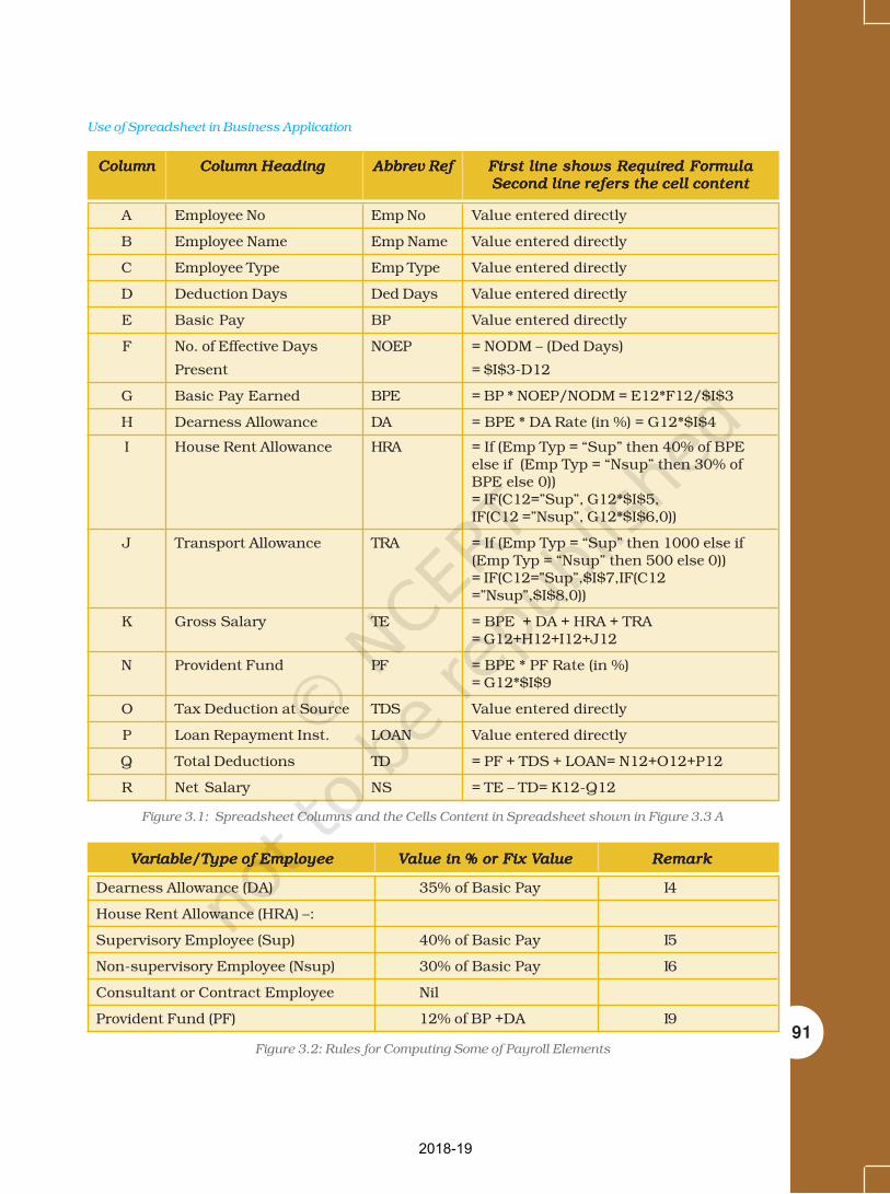
Use of Spreadsheet in Business Application
91
ColumnColumnColumnColumnColumn Column HeadingColumn HeadingColumn HeadingColumn HeadingColumn Heading Abbrev RefAbbrev RefAbbrev RefAbbrev RefAbbrev Ref First line shows RequirFirst line shows RequirFirst line shows RequirFirst line shows RequirFirst line shows Required Fored Fored Fored Fored FormulamulamulamulamulaSecond line refers the cell contentSecond line refers the cell contentSecond line refers the cell contentSecond line refers the cell contentSecond line refers the cell content
A Employee No Emp No Value entered directly
B Employee Name Emp Name Value entered directly
C Employee Type Emp Type Value entered directly
D Deduction Days Ded Days Value entered directly
E Basic Pay BP Value entered directly
F No. of Effective Days NOEP = NODM – (Ded Days)
Present = $I$3-D12
G Basic Pay Earned BPE = BP * NOEP/NODM = E12*F12/$I$3
H Dearness Allowance DA = BPE * DA Rate (in %) = G12*$I$4
I House Rent Allowance HRA = If (Emp Typ = “Sup” then 40% of BPEelse if (Emp Typ = “Nsup” then 30% ofBPE else 0))= IF(C12=”Sup”, G12*$I$5,IF(C12 =”Nsup”, G12*$I$6,0))
J Transport Allowance TRA = If (Emp Typ = “Sup” then 1000 else if(Emp Typ = “Nsup” then 500 else 0))= IF(C12=”Sup”,$I$7,IF(C12=”Nsup”,$I$8,0))
K Gross Salary TE = BPE + DA + HRA + TRA= G12+H12+I12+J12
N Provident Fund PF = BPE * PF Rate (in %)= G12*$I$9
O Tax Deduction at Source TDS Value entered directly
P Loan Repayment Inst. LOAN Value entered directly
Q Total Deductions TD = PF + TDS + LOAN= N12+O12+P12
R Net Salary NS = TE – TD= K12-Q12
Figure 3.1: Spreadsheet Columns and the Cells Content in Spreadsheet shown in Figure 3.3 A
VVVVVariable/Tariable/Tariable/Tariable/Tariable/Type of Employeeype of Employeeype of Employeeype of Employeeype of Employee VVVVValue in % or Fix Value in % or Fix Value in % or Fix Value in % or Fix Value in % or Fix Valuealuealuealuealue RemarkRemarkRemarkRemarkRemark
Dearness Allowance (DA) 35% of Basic Pay I4
House Rent Allowance (HRA) –:
Supervisory Employee (Sup) 40% of Basic Pay I5
Non-supervisory Employee (Nsup) 30% of Basic Pay I6
Consultant or Contract Employee Nil
Provident Fund (PF) 12% of BP +DA I9
Figure 3.2: Rules for Computing Some of Payroll Elements
2018-19

92
Computerised Accounting System
The following spreadsheet shows columns A to K in Figure 3.3 a; whilecolumns L to P are shown in Figure 3.3 b. For reference, columns Aand B are repeated in columns L and M in Figure 3.3 b for referenceonly.
Figure 3.3 a : Partial Spreadsheet Showing Payroll List upto Gross Salary
Figure 3.3 (b) : Partial Spreadsheet for calculation of Deductions & Net Salary
2018-19

Use of Spreadsheet in Business Application
93
3.2 ASSET ACCOUNTING
In this section, we shall be discussing the computation of amount ofdepreciation to be charged on assets.
3.2.1 INTRODUCTION
Assets are resources of the organisation, which can be classified intofixed and current assets. Fixed assets are long-term assets and provideproductive capability to the firm. The examples of fixed assets areland, building, plant & machinery, etc. It includes both tangible andintangible assets. Tangible assets are physical in nature, which haveform, shape and size. Intangible assets are resources capable of addingvalue but do not have a physical dimension such as patents, copyrights,trade mark, etc.
The depreciation on fixed assets is provided to recognise the cost ofthe asset consumed during an accounting period since the life of suchassets extends beyond single accounting year. Usually, depreciation isnot provided on free hold land.
Total Amount of Depreciation = Acquisition Cost – Salvage Value(Over Life of the Asset)
Year-to-date depreciation is the accumulated depreciation from thedate to which the asset is put to use till the current accounting year.
Depreciation is calculated according to the policy of the organisation.There are basically two methods, namely the Straight Line Method(SLM) and the Written Down Value Method (WDV). We had studieddepreciation in our previous standard (XIth Standard) in AccountancyBook Part I.
We will recall that asset accounting requires maintenance of assetregister, computation of depreciation and preparation of schedule offixed assets for reporting in the balance sheet as part of the annualaccounts. In order to prepare this report the depreciation calculationsheet is also to be prepared.
3.2.2 COMPUTERISED ASSET ACCOUNTING
Assets are classified into the following categories:
• Goodwill
• Land: Free-hold land and Lease-hold land
• Building: Factory building, Office building, and Residential building
Year-to-date depreciation is the accumulated depreciation from thedate to which the asset is put to use till the current accounting year.
2018-19

94
Computerised Accounting System
• Plant and Machinery
• Furniture and Fixtures
• Vehicles
• Capital work in progress
• Others
The Companies Act, 1956 in Schedule-14 lists the rate of depreciation
to be used for different class of assets under Straight Line Method
(SLM) and Written Down Value Method (WDV). The prescribed rates
are different under two methods. For reporting purposes, corporate
enterprises may use either of the method and applicable rates. Let us
now understand the computation of depreciation using the two methods.
3.2.2.1 Straight Line Method (SLM)
The following is the formula for computation of depreciation:
• Acquisition Cost = Purchase Value + Other expenses, such asTransportation Expenses, Installation Expenses and Pre-operatingExpenses
• Total Depreciable Amount = Acquisition Cost - Salvage Value
•Total Depreciable Amount
Straight Line Depreciaion = Expected Useful Life
•Straight Line Depreciation
Rate of Depreciaion = × 100Total Depreciable Amount
ExampleExampleExampleExampleExample
The depreciation calculation (using SLM) is done using the Excel
spreadsheet, which is shown in Fig. 3.5 a and Fig. 3.5 b in two parts
due to the limitation of the page width. In each of the spreadsheet
column, either a value is entered directly or else it is computed using
a formula. Such data are given in Figure 3.4.
Different data elements are arranged in the spreadsheet as follows:
• Year Beginning Date is entered in cell-C3
• Year End Date is entered in cell-F3
• First-Half Year End Date is entered in cell-E3
The salvage value of an asset is the value, which is realisable at theend of its useful life.
2018-19

Use of Spreadsheet in Business Application
95
Figure 3.5(a) : Partial Spreadsheet Columns for Calculation of Depreiation by SL Method
The depreciation is computed by straightline method using the built-in spreadsheet function SLN in column-K. The spreadsheets are shownin Figure 3.5(a) and Figure 3.5(b).
The above-mentioned computations and spreadsheets (shown in twoparts due to the constraint in the page width) give an idea of theprocess of depreciation calculation using SLM function. The spreadsheet
Figure 3.4: Column Items and their contents referred to in the Spreadsheet
ColumnColumnColumnColumnColumn Column HeadingColumn HeadingColumn HeadingColumn HeadingColumn Heading Abbrev RefAbbrev RefAbbrev RefAbbrev RefAbbrev Ref First line shows RequirFirst line shows RequirFirst line shows RequirFirst line shows RequirFirst line shows Required Fored Fored Fored Fored FormulamulamulamulamulaSecond line refers the cell contentSecond line refers the cell contentSecond line refers the cell contentSecond line refers the cell contentSecond line refers the cell content
A Asset Name Asset Name Value entered directly
B Date of Purchase Pur. Date Value entered directly
C Date of Installation Inst. Date Value entered directly
D Cost of Purchase Pur. Cost Value entered directly
E Installation Expenses Inst. Exp. Value entered directly
F Pre-operating Pre-op Exp Value entered directlyExpenses
G Cost to Use Cost to Use = (Cost of Purchase) + (Installation Expenses)+ (Pre-operating Expenses) = D5+E5+F5
H Salvage Value Salvage Val Value entered directly
I Life of Asset in Years Life in Yrs Value entered directly
K Depreciation Amount Depr. =SLN(G5,H11,I11)
Figure 3.5(b) : Partial Spreadsheet Columns for Calculation of Depreciation by SL Method
H I J K
2018-19
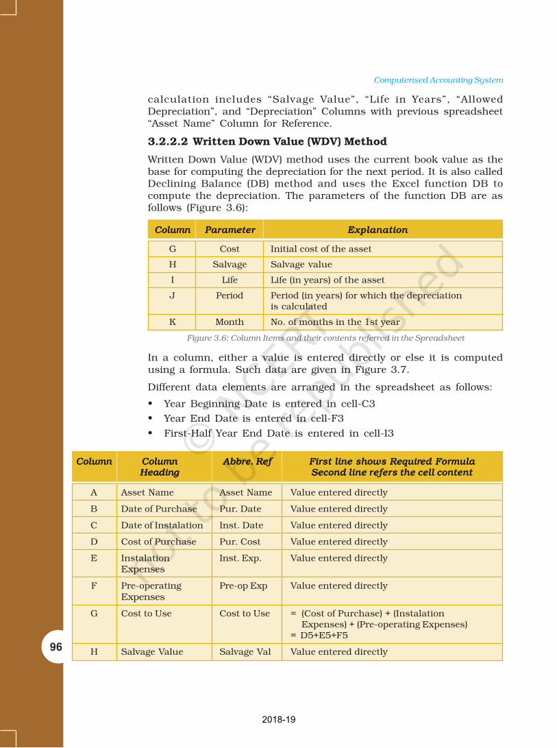
96
Computerised Accounting System
calculation includes “Salvage Value”, “Life in Years”, “AllowedDepreciation”, and “Depreciation” Columns with previous spreadsheet“Asset Name” Column for Reference.
3.2.2.2 Written Down Value (WDV) Method
Written Down Value (WDV) method uses the current book value as thebase for computing the depreciation for the next period. It is also calledDeclining Balance (DB) method and uses the Excel function DB tocompute the depreciation. The parameters of the function DB are asfollows (Figure 3.6):
In a column, either a value is entered directly or else it is computedusing a formula. Such data are given in Figure 3.7.
Different data elements are arranged in the spreadsheet as follows:
• Year Beginning Date is entered in cell-C3
• Year End Date is entered in cell-F3
• First-Half Year End Date is entered in cell-I3
ColumnColumnColumnColumnColumn ParameterParameterParameterParameterParameter ExplanationExplanationExplanationExplanationExplanation
G Cost Initial cost of the asset
H Salvage Salvage value
I Life Life (in years) of the asset
J Period Period (in years) for which the depreciationis calculated
K Month No. of months in the 1st year
Figure 3.6: Column Items and their contents referred in the Spreadsheet
ColumnColumnColumnColumnColumn ColumnColumnColumnColumnColumn Abbre. RefAbbre. RefAbbre. RefAbbre. RefAbbre. Ref First line shows RequirFirst line shows RequirFirst line shows RequirFirst line shows RequirFirst line shows Required Fored Fored Fored Fored FormulamulamulamulamulaHeadingHeadingHeadingHeadingHeading Second line refers the cell contentSecond line refers the cell contentSecond line refers the cell contentSecond line refers the cell contentSecond line refers the cell content
A Asset Name Asset Name Value entered directly
B Date of Purchase Pur. Date Value entered directly
C Date of Instalation Inst. Date Value entered directly
D Cost of Purchase Pur. Cost Value entered directly
E Instalation Inst. Exp. Value entered directlyExpenses
F Pre-operating Pre-op Exp Value entered directlyExpenses
G Cost to Use Cost to Use = (Cost of Purchase) + (InstalationExpenses) + (Pre-operating Expenses)
= D5+E5+F5
H Salvage Value Salvage Val Value entered directly
2018-19

Use of Spreadsheet in Business Application
97
ColumnColumnColumnColumnColumn ColumnColumnColumnColumnColumn Abbre. RefAbbre. RefAbbre. RefAbbre. RefAbbre. Ref First line shows RequirFirst line shows RequirFirst line shows RequirFirst line shows RequirFirst line shows Required Fored Fored Fored Fored FormulamulamulamulamulaHeadingHeadingHeadingHeadingHeading Second line refers the cell contentSecond line refers the cell contentSecond line refers the cell contentSecond line refers the cell contentSecond line refers the cell content
I Life of Asset in Life in Yrs Value entered directlyYears
J Period (in Years) Period If (Instalation of asset was done afterfor which Depr. March) then take (Current Year) – (Year ofis to be computed Instalation) else take one addl. Year.
= IF (MONTH(C5) > 3,(YEAR($F$3)-YEAR(C5)),(YEAR($F$3)-YEAR(C5))+1)
K Months in 1st Year Months in No. of months between (Yr-End-Dt in 1st Yr)(i.e. the year of 1st Yr & (Inst.Date)installation) = ROUND((L5-C5)/30,0)
L Year-end Date in Yr-End-Dt If (Inst. Date) was Between Jan and Mar,1st Year (Reqd. in 1st Yr Take it as 31st Mar of (Year of Inst. Date)to compute Else Take it as Next Year.column-K) = IF(AND(MONTH(C5)>0,MONTH(C5) <4),
DATE(YEAR(C5),3,31),DATE(YEAR(C5)+1,3,31))
M Depreciation Depr. Parameters of DB function as explainedabove= DB(G5,H5,I5,J5,K5)
Figure 3.7: Column Items and their Contents used in Spreadsheet (in Figure 3.8 a and b)
The spreadsheet is divided in two parts; first part shows columns A toG in Figure 3.8 a; while second part shows columns H to M are shownin Figure 3.8 b. The “Asset Name” is repeated in both the figures:
Figure 3.8 b : Partial Spreadsheet Columns for Calculation of Depreciation by WDV Method
Figure 3.8 a : Partial Spreadsheet Columns for Calculation of Depreciation by WDV Method
2018-19

98
Computerised Accounting System
The above-mentioned computations and spreadsheets (shown in twoparts due to the constraint in the page width) give an idea of theprocess of depreciation calculation using WDV function. Thespreadsheet calculation includes “Salvage Value”, “Life in Years”,“Allowed Depreciation”, and “Depreciation” Columns with previousspreadsheet “Asset Name” Column for Reference.
3.2.2.3 Schedule Forming Part of the Balance Sheet
The details of various columns are given in the following table:
The spreadsheet is divided in two parts; first part shows columns A toE in Figure 3.10 a; while second part shows columns F to K are shownin Figure 3.10 b. The “Asset Name” is repeated in both the figures:
ColumnColumnColumnColumnColumn ColumnColumnColumnColumnColumn UnderUnderUnderUnderUnder First line shows RequirFirst line shows RequirFirst line shows RequirFirst line shows RequirFirst line shows Required Fored Fored Fored Fored FormulamulamulamulamulaHeadingHeadingHeadingHeadingHeading Second line refers the cell contentSecond line refers the cell contentSecond line refers the cell contentSecond line refers the cell contentSecond line refers the cell content
A Description Value entered directly
B As at Apr 1, 2008 Gross Block Value entered directly
C Additions/Adjustments Gross Block Value entered directly
D Deductions/Adjustments Gross Block Value entered directly
E As at Mar 31, 2009 Gross Block = Op. Bal + Additions/Adjustments= B8+C8-D8
F As at Apr 1, 2008 Depreciation Value entered directly
G Additions Depreciation Value Transferred from DepreciationComputation Spreadsheet
H Deductions Depreciation Value entered directly
I As at Mar 31, 2009 Depreciation = Op. Bal + Additions – Deductions= F8+G8-H8
J As at Apr 1, 2008 Net Block = Gross Block – Depreciation as onApr 1, 2008
= B7–F7
K As at Mar 31, 2009 Net Block = Gross Block – Depreciation as onMar 31, 2009
= E7-I7
Figure 3.9: Column Items and their Contents used in Spreadsheet (in Figure 3.10 a and b)
Figure 3.10 a: Spreadsheet Containing Fixed Asset Schedule Showing Gross Block
2018-19

Use of Spreadsheet in Business Application
99
Figure 3.10 b: Spreadsheet Containing Fixed Asset Schedule Showing Depreciation and Net Block
The above-mentioned computations and spreadsheets (shown in twoparts due to the constraint in the page width) give an idea of theprocess of Schedule Forming Part of the balance sheet.
3.3 LOAN REPAYMENT SCHEDULE
3.3.1 LOAN
Loan is a sum of borrowed money (termed as principal amount) for aspecified period at a pre-specified rate of interest. The loan is repaidthrough a number of periodic (usually monthly) repayment instalmentsover the loan repayment period.
3.3.1.1 Calculating Interest and Repayments of Loan
Computation of repayment installments is an iterative process. TheExcel’s built-in function, PMT can be used to compute monthlyinstalments of repayment of loan. The parameters of the function PMTare as follows:
The layout of the spreadsheet for loan repayment calculation is givenin Figure 3.13. In each column of the spreadsheet, either a value isentered directly or else it is computed using a formula. Such data aregiven in Figure 3.12.
ParameterParameterParameterParameterParameter ExplanationExplanationExplanationExplanationExplanation
Rate Interest rate per period for the loan
Nper Total number of payments for the loan. Its unit (e.g. year)should match with the unit of the interest rate.
Pv Present value, i.e. the loan amount
Fv Future value, which is taken as 0, is the balance at theend of the loan period
Type Whether payment is made at the beginning (value=1) orat the end (value=0) of the period
Figure 3.11 Explanation of Parameters of Excel’s PMT Function
2018-19

100
Computerised Accounting System
The following two examples are considered for computation of repaymentschedule in the spreadsheet shown in Figure 3.13.
Example 1Example 1Example 1Example 1Example 1
A bank has given loan of Rs. 1, 00,000 to a customer for the purchaseof a Plasma TV on April 1, 2007 @ 10% interest rate for a period of twoyears. The loan is to be repaid in 24 monthly instalments.
Example 2Example 2Example 2Example 2Example 2
Ajay has been sanctioned the bank loan of Rs. 2, 50,000 for the purchaseof a car on May 15, 2008. The loan carries the rate of interest @ 11%and it is to be repaid in 36 monthly instalments.
Figure 3.12: Column Items and their Contents in Spreadsheet
ColumnColumnColumnColumnColumn Column HeadingColumn HeadingColumn HeadingColumn HeadingColumn Heading First line shows RequirFirst line shows RequirFirst line shows RequirFirst line shows RequirFirst line shows Required Fored Fored Fored Fored FormulamulamulamulamulaSecond line refers the cell contentSecond line refers the cell contentSecond line refers the cell contentSecond line refers the cell contentSecond line refers the cell content
A Loan Amt. Value entered directly
B Loan Disbursement Date. Value entered directly
C Period of Loan (in Yrs). Value entered directly
D Rate of Interest. Value entered directly
E Future Value. Value entered directly
F Yearly Installment Amt. = PMT(D6,C6,-A6,0,1)
G Monthly Installment Amt. =F6/12
Figure 3.13: Spreadsheet Containing Loan Repayment Schedule
Why is FV taken as zero (0) in the above calculations?
At the end of the loan period, the (balance) amount payable will bezero assuming that the repayments are made on regular basis.Therefore, the future value (FV) is taken as zero.
2018-19

Use of Spreadsheet in Business Application
101
SummarySummarySummarySummarySummary
• MS-Excel is an easy and useful tool for various calculations carried out on spreadsheets.In this chapter, three examples have been taken to illustrate the ease and utility ofspreadsheets. These examples are Payroll Calculation, Fixed Asset Accounting, and LoanRepayment Schedule.
• The first step in using spreadsheet is to list out the elements of the application. For eachelement, it is determined whether a direct value is to be entered or else it is to be computedusing a formula.
• Excel has a rich library of various built-in functions including financial functions, whichcan be directly used to carry out various (otherwise complex) calculations. A formula mayuse one or more such functions.
• In these applications, some of the formulae use absolute address. The absolute address isused for those cells whose content should not change while the formula containing suchcells is copied to other cells.
• If-function is also used in these applications. If-function is used to implement differentaction corresponding to different conditions.
• The Excel functions SLN and DB are used for computation of depreciation using StraightLine Method (SLM) and Written Down Value Method (WDVM), respectively. WDV Method isalso termed as declining balance (DB) method.
• The function PMT is used to compute the loan repayment schedule.
EXERCISE
Q1. MULTIPLE CHOICE QUESTIONS
1. Which of the following options in a financial function indicates the interest fora period?
a. FV.
b. PV.
c. Nper.
d. Rate.
2. Which of the following arguments in a financial function represents the totalnumber of payments?
a. FV.
b. PV.
c. Nper.
d. Rate.
2018-19

102
Computerised Accounting System
3. What category of functions is used in this formula:=PMT(C10/12,C8,C9,1)
a. Logical.
b. Financial.
c. Payment.
d. Statistical.
4. When Extend Selection is active, what is the keyboard shortcut for selectingall data up to and including the last row?
a. [Ctrl]+[Down Arrow].
b. [Ctrl]+[Home].
c. [Ctrl]+[Shift].
d. [Ctrl]+[Up Arrow].
5. Which formula would result in TRUE if C4 is less than 10 and D4 is less than100?
a. =AND(C4>10, D4>10).
b. =AND(C4>10, C4<100).
c. =AND(C4>10, D4<10).
d. =AND(C4<10, D4<100).
6. Which of these is not an argument of the IF function?
a. Logical_test.
b. Value_if_false.
c. Value_when_false.
d. Value_if_true.
7. In what cell is the Rate for PMT function where = PMT (C8, C9, C10, C11,C12)?
a. C8.
b. C9.
c. C10.
d. C12.
Q2. ANSWER THE FOLLOWING QUESTIONS
1. What is the meaning of PV?
2. State the usage of FV?
3. What is the purpose of DB function?
2018-19

Use of Spreadsheet in Business Application
103
4. If an investment of Rs. 1,000 is made today, ascertain its Future Value (FV)after 2 years if the rate of interest is taken as 10%?
5. If a sum of Rs. 1000 is likely to be earned after 3 years, calculate its presentvalue (PV).
6. What is the difference between WDV method and SLM method of depreciation?
7. Describe the two basic methods of depreciation. What functions of Excel areused for computation of depreciation?
8. Explain the importance of absolute and relative addresses. What is the basisof using relative address and absolute address?
SKILL REVIEW1. In columns F, G, H, I, J, and N of the Payroll spreadsheet shown in Figure
3.3 (a) and Figure 3.3 (b) the absolute addresses are used. What will happenif relative addresses are used instead of absolute addresses?
2. In columns g of the spreadsheet shown in Figure 3.8 b for the depreciationcalculation using WDV method (i.e. using DB function), the absolute addressesof cell F3 is used. Taking relative address of F3 instead of its absolute addresswill lead to wrong result when the formula is copied. Explain the reason andwrite down the values copied along with the correct values, which shouldhave been copied.
3. Prepare attendance record in a spreadsheet for a class of 25 student’s monthwise for 10 months. Calculate the percentage of presence for each studentevery month. Prepare a month wise summary of every student and calculatethe overall percentage of presence.
4. Use spreadsheet to prepare class timetable. It should compute and check thetotal number of lectures, tutorials and lab practical sessions allocated foreach subject. It should also compute and check the total number of hours ofengagement for each teacher.
5. Prepare the worksheets yourself for examples used in sections 3.1, 3.2, 3.3and 3.4 respectively. Add two new more records in each worksheet (with yourown assumed values) and verify whether the computations are correct.
6. Create a worksheet to keep a record of employees of M/s OpportunitiesCompany. Employee details should include Name of Employee, Designationand Basic Salary. Enter 50 records. Calculate Dearness Allowance (DA) as37.5% of Basic Salary, House Rent Allowance (HRA) 22.5% of Basic Salary,Provident Fund (PF) as 12% of Basic Salary, Gross Salary as Basic Salary +DA+HRA. The Income Tax (IT) as 20% of Gross Salary and Net Salary is GrossSalary – (PF+IT) for each employee. Calculate also Total Salary, Average Salary,Maximum Salary and Minimum Salary paid by the company.
7. In Section-3.3, the loan instalment is computed for a given amount of loanrepayable over a specified period at a specified rate of interest. Modify thisexercise by fixing the loan instalment amount and compute the loan periodusing the PMT function.
2018-19

104
Computerised Accounting System
ANSWERS
1. b 2. c 3. b 4. c 5. d 6. c 7. a
2018-19

GRAPHS AND CHARTS
FOR BUSINESS DATA
Introduction
4
In the previous chapter, you were introduced to
the basic features of spreadsheet and use of
spreadsheet in accounting. Quite often, we have
to present the data for communication of the
accounting information. If mass of data is presented
in the raw form, it may not be easily
understandable. It is rightly said, “A picture is
worth more than thousand words”. This chapter
seeks to explain the method of preparing graphs,
charts and diagrams showing the data through
the use of Excel as a tool.
4.1 GRAPHS AND CHARTS
A graph is a pictorial representation of data, which
has at least 2 dimensional relationship. Therefore,
a graph has at least two axes, X and Y. X-axis is
usually horizontal while Y-axis is vertical. A graph
may either be a singleline graph or a multiple-
line graph. For ease and enhancing of clarity,
different types of lines and different shades of
Colours can be used for preparing a multiple-line
graph.
A pie chart represents multiple sub-groups of
single variable. A bar diagram depicts two or more
variables.
After studying this chapter, you will be
able to:
• represent data in graphical form
in charts & diagrams through
Excel.
• use accounting data for graphical
representation.
2018-19

106
Computerised Accounting System
Figure 4.1 shows different types of graphs and charts which can be
prepared with the help of the commands or standard tools given in
toolbar.
Figure 4.1: Various types of graph and charts
Using the MS Excel 2007 we can create a basic chart by clickingthe chart type that we want on the Microsoft Office Fluent user interfaceRibbon, as shown in Figure 4.2. Remember these following steps whichare already explained in previous chapter.
Figure 4.2: Tools for various types of graphs
2018-19
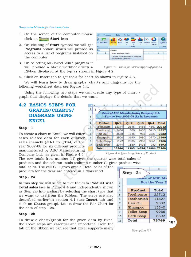
Graphs and Charts for Business Data
107
1. On the screen of the computer mouse
click on Start Icon
2. On clicking of Start symbol we will getPrograms option; which will provide usaccess to a list of programs installed onthe computer.
3. On selecting MS Excel 2007 program itwill provide a blank workbook with aRibbon displayed at the top as shown in Figure 4.2.
4. Click on Insert tab to get tools for chart as shown in Figure 4.3.
We will learn how to draw graphs, charts and diagrams for thefollowing worksheet data see Figure 4.4.
Using the following two steps we can create any type of chart /graph that displays the details that we want.
4.2 BASICS STEPS FORGRAPHS/CHARTS/DIAGRAMS USINGEXCEL
Step - 1
To create a chart in Excel; we will entersales related data for each quartersales (namely QTR1 to QTR4) of theyear 2007-08 for six different productsmanufactured by ABC ManufacturingCompany Ltd. (as given in Figure 4.4)The row totals (row number 11) gives the quarter wise total sales ofproducts and the column totals (column number G) gives product wisetotal sales. The cell G11 gives over all total sales of theproducts for the year are entered in a worksheet.
Step - 2a
In this step we will select to plot the data Product wiseTotal sales (see in Figure 4.4 and independently shownas Step 2a) into a chart by selecting the chart type thatwe want to use from the Ribbon. The steps are alsodescribed earlier in section 4.1 (use Insert tab andclick on Charts group). Let us draw the Bar Chart forthe data of step - 2a.
Step - 2b
To draw a chart/graph for the given data by Excelthe above steps are essential and important. From thetab on the ribbon we can see that Excel supports many
Figure 4.3 Tools for various types of graphs
Figure 4.4 Quarterly Sales of Product
1
No caption ???
2018-19

108
Computerised Accounting System
types of charts to display data inmeaningful ways.
Let us prepare a new chart from thesame worksheet to display total sales foreach quarter. The data in the worksheet isto be reorganised for the purpose of chartpreparation and as mentioned above,graph/chart will be prepared in similar twosteps as described above (Figure 4.5).
Period Total Sales
Qtr1 25844
Qtr2 11295
Qtr3 14744
Qtr4 21886
Total 73769
To create a chartor to change anexisting chart, weselect variety ofchart types (such as
a column chart or pie chart) and their sub-types (such as a stackedcolumn chart or a pie in 3-D chart) from the ribbon. We can also createa combination of chart by using more than one chart type in any chart.This could be possible once we understand the elements of the chartand the formatting of the chart.
4.2.1 ELEMENTS OF A CHART/GRAPH
Figure 4.5
A chart/graph are a pictorialpresentation of data. To understandand explain the chart/graph we willlearn all basic elements of thechart. These chart/graph elementsare given in Figures 4.6 and 4.7.
1. The chart area: The entire chartincluding all elements.
2. The plot area: In a 2-D chart,the area is bounded by the X and Yaxes. In a 3-D chart, the area isbounded by the three (X, Y and Z)axes.
Figure 4.6
2018-19

Graphs and Charts for Business Data
109
3. The data points: Individual values plotted in a chart and representedby bars, columns, lines, pie or various other shapes are called datamarkers. Data markers of the same colour constitute a data series.The data series are related data points that are plotted in the chart/graph. Each data series in a chart is shown in a unique colour orpattern or both. Its identification is given by the legend. There may bemore than one data series in a chart/graph.
4. The horizontal (category) and vertical (value) axis: The x-axis isusually the horizontal line which contains categories (independentvalues or categories) and y-axis is usually the verticals which containsdata (dependent values).
5. The legend: It is an identifier of a piece of information shown in thechart/graph. The legends are assigned to the data series or differentcategories in a chart (Figure 4.7).
6. A chart and axes titles: Descriptive text for chart title (6-A) andaxis title (6-B) as shown in Figure 4.6.
7. A data label: This provides additional information about a datamarker to identify the details of data point in a data series.
Some of the elements are displayed by default when we prepare thechart/graph; others can be added as needed. It is also possible tochange the format or display of the chart/graph as desired.
Figure 4.7
4.2.2 FORMATTING OF CHART
4.2.2.1 Formatting the Chart (using design option)
As referred in earlier section 4.2.1 above; in this section we will learnhow the elements of a chart such as plot area, X-axis, Y-axis, data,
2018-19

110
Computerised Accounting System
titles, labels, legends and gridline as shown in Figure 4.7 can beformatted and edited as per the requirement. Click anywhere in thechart. This will display the Chart Tools, adding the Design, Layout,and Format tabs (Figure 4.8a).
Using Design option we can change the look of a chart. In theDesign dialog box, we can click to change chart type, chart layoutsand chart styles. One of the options provide for 2-d chart to swap thecolumn data to row data and row data to column data. The steps areas follows:
In a chart (Figure 4.7) click the chart element to change, or do thefollowing to select the chart element from a list of chart elements:
Figure 4.8 (a)
1. Click anywhere in the chart(Figure 4.7). This will displaythe Chart Tools, adding theDesign, Layout, and Formattabs.
2. On the Design tab, in theData group, click the arrowat the Switch Row/Columnbox.
3. This will swap the chart/graph from X-axis (Product)to X-axis (Quarterly)(Figure4.8(b).
4.2.2.2 Changing the format of a selected chart element
In the same chart, click the chart element to change, or do the followingto select the chart element from a list of chart elements:
Figure 4.8 (b)
Figure 4.8 (c)
1. Click anywhere in the chart. This will display the Chart Tools,adding the Design, Layout, and Format tabs (Figure 4.8(c).
2018-19

Graphs and Charts for Business Data
111
2. On the Format tab, in the Current Selection group,click the arrow next to the Chart Elements box, andthen select the chart element which requires toformat.
3. On the Format tab, in the Current Selection group,click the Format Selection (Figure 4.8(d)).
4. In the Format <Chart Element> dialog box, click acategory, and then select the formatting options.
Changing the shape styleChanging the shape styleChanging the shape styleChanging the shape styleChanging the shape style
1. On the Format tab, in the Shape Styles group, do one of thefollowing:
• To see all available shape styles,click the More button.
• To apply a pre- defined shapestyle, in the shape style box, clickthe style that we want.
• To apply a different shape fill, click Shape Fill, and then do oneof the following: (Figure 4.8(e))
To use a different fill Colour, under Theme Colours or StandardColours, left click the select Colour.
To remove the Colour from the selected chart element, clickNo Fill.
To use a fill Colour that is not available under Theme Coloursor Standard Colours click More Fill Colours. In the Coloursdialog box, specify the Colour that we want to use on theStandard or Custom tab, and then click OK. Custom fillColours are added under Recent Colours can also be used.
To fill the shape with a picture, click Picture. In the InsertPicture dialog box, click the picture to use, and then clickInsert.
To use a gradient effect for the selected fill Colour, clickGradient, and then under Variations, click the gradient styleto be used. For additional gradient styles, click MoreGradients, and then in the Fill category, click the gradientoptions that to use.
To use a texture fill, click Texture, and then click the textureto use.
Changing the Shape OutlineChanging the Shape OutlineChanging the Shape OutlineChanging the Shape OutlineChanging the Shape Outline
• To apply a different shape outline, click Shape Outline, and thendo one of the following:
To use a different outline Colour, under Theme Colours orStandard Colours, click the Colour to use.
Figure 4.8 (d)
Figure 4.8 (e)
2018-19

112
Computerised Accounting System
To remove the outline Colour from the selected chart element,click No Outline. If the selected element is a line, the line will nolonger be visible on the chart.
To use an outline Colour that is not available under ThemeColours or Standard Colours click More Outline Colours. Inthe Colours dialog box, specify the Colour that to use on theStandard or Custom tab, and then click OK. Custom outlineColours are added under Recent Colours can be used again.
To change the weight (thickness) of a line or border, click Weightoption, and then select the line that we wish to use. For additionalline style or border style options, click on More Lines, and thenclick the line style or border style options.
To use broken line (dash–dash) or border, click Dashes, andthen click the dash type to use. For additional dash-type options,click on More Lines, and then click the selected dash.
To add arrows to lines, click Arrows, and then click the arrowstyle for borders cannot be used. For additional arrow style orborder style options, click More Arrows, and then click the arrowsetting.
To apply a different shape effect, click Shape Effects, click anchosen effect, and then select the type of effect.
The shape effects depend on the chart element that we select suchas Pre-set, reflection, and bevel. The shape effects are not availablefor all chart elements.
Changing the text forChanging the text forChanging the text forChanging the text forChanging the text formatmatmatmatmat
To format the text in chart elements, we can use regular text formattingoptions, or we can apply a WordArt format.
1. Click the chart element that contains the text to format.
2. Right-click the text or select the text to format, and then do one ofthe following:
Click the formatting options that we want on the Mini toolbar.
On the Home tab, in the Font group, click the formatting buttonsthat we want to use.
To use WordArt styles to format text use chart elements in thefollowing steps: (Figure 4.8(f)
1. In a chart, click the chart element thatcontains the text to be changed, or do thefollowing to select the chart element from alist of chart elements:
2. Click anywhere in the chart.
3. This displays the Chart Tools, adding theDesign, Layout, and Format tabs.
Figure 4.8 (f)
2018-19

Graphs and Charts for Business Data
113
4. On the Format tab, in the Current Selection group, click the arrownext to the Chart Elements box, and then select the chart elementthat to format.
5. On the Format tab, in the WordArt Styles group, doone of the following: (Figure 4.8(g))
• To see all available WordArt styles, click the Morebutton.
We get options for Text related formatting
Text Fill
Text Outline
Shadow
3-D Format
3-D Rotation
Text Box
4.2.2.3 Changing the layout of the chart element
In the same chart, click the chart element to change, or do the followingto select the chart element from a list of chart elements:
1. On the Layout tab, we can insert different Clip Arts, Picture, datalabels, grids etc.
2. In the Format <Chart Element> dialog box, click a category, andthen select the formatting options.
4.2.3 CHANGE THE CHART TYPE
A chart can be changed to another type ofchart to get different look and purpose. Forexample, the chart shown in Figure 4.5 canbe changed to Pie a chart (Figure 4.9) byusing the chart tool as given on the Ribboninterface and in Figure 4.2. The every Pie ofthe chart represents the size of total sales ineach quarter proportionately and whole Piechart displays sum of all the Pies equals to100%.
This is the easiest method to change fromcolumn chart or bar chart to Pie chart because
Figure 4.8 (h)
Figure 4.9
Figure 4.8 (g)
2018-19

114
Computerised Accounting System
• Only one data series isused to plot.
• The plotted data valuesare positive.
• The data values are notequal to zero also.
Note that in Excel software Pie chart cannot plotmore than seven catgories. The categories representthe parts of whole Pie.
Steps for creating a Pie ChartSteps for creating a Pie ChartSteps for creating a Pie ChartSteps for creating a Pie ChartSteps for creating a Pie Chart
1. Enter the data in a worksheet.
2. Select the data from two (consecutive) columnsonly.
3. Select the chart type Pie from the ribbon.
4. Under Pie types select 3-D Pie option
5. Click the plot are of Pie chart this displays theChart Tools, adding the Design, Layout, andFormat tabs.
6. On the Design tab, in the Chart Layouts group,select the layout to use.
7. On the Design tab, in the Chart Styles group,click the chart style.
8. On the Format tab, in the Shape Styles group,click Shape Effects, and then click Bevel.
9. Click 3-D Options, and then under Bevel, clickthe Top and Bottom bevel options.
10.In the Width and Height boxes for Top andBottom bevel options, type the point size.
11.Under Surface, click Material, and then clickthe material option.
12.Click Close.
13.On the Format tab, in the Shape Styles group,click Shape Effects, and then click Shadow.
14.Under Outer, Inner, or Perspective, click theshadow option.
15.To rotate the chart for a better perspective, selectthe plot area, and then on the Format tab in theCurrent Selection group, click FormatSelection.
Figure 4.9 (a)
Figure 4.9 (b)
Figure 4.9 (c)
Figure 4.9 (d)
Figure 4.9 (e)
Figure 4.9 (f)
Figure 4.9 (g)
2018-19

Graphs and Charts for Business Data
115
16.Under Angle of first slice, drag the slider to the degree of rotationthat you want, or type a value between 0 (zero) and 360 to specifythe angle of the first slice to appear, and then click Close.
17.Click the chart area of the chart.
18.On the Format tab, in the Shape Styles group, click Shape Effects,and then click Bevel.
19.Under Bevel, select the bevel option.
20.To use theme colors that are different from the default theme thatis applied the workbook, do the following:
a. On the Page Layout tab, in the Themes group, click Themes.
b. Under Built-in, click the theme to use.
4.2.4 RESIZING OF CHART/GRAPH
Resizing of the chart means changing size of the chart as desired. Thisoption can be used independently for the fonts, title, legends easily.The first step is to select the chart by clicking the left button of themouse. Move the cursor on the corners or middle of the borders of thechart/graph which will provide the figure (the cursor will take theshape of a two headed arrow). By pressing the left button and drag/pull as desired to resize the chart as shown by the red circle in theFigure 4.9a.
4.2.5 2D - 3D CHARTS/GRAPHS
To create graphs we use data which are plotted in twodimensional (2D) format ( X- axis and Y-axis) as shownin the Figure 4.7. Where as
• Horizontal dimension is X-axis(contains categories)
• Vertical dimension is Y-axis(contains data)
When we plot the data on 2-D type of graph; theknown value goes on the X-axis (independent) andderived (dependent variable) value on Y-axis. Forexample monthly demand of products (in Rs.); then onX-axis we will put Month and on Y-axis we will put thedata values for demand.
In the graph sometimes we have to present negativevalues also, which can be put on the opposite side of theaxes from origin (Figure 4.10). The intersection of boththe axes (X-axis and Y-axis) is called the origin (O) of thegraph. We can put on the right side of the origin positivevalues and on left side of the origin negative values ofdata on X-axis. Similarly upper ward side of origin showspositive values and down ward side of the origin showsnegative values of data Y-axis. For example, if we havedata about monthly profit and loss to be plotted on graph;
Figure 4.10
Figure 4.11(a)
2018-19

116
Computerised Accounting System
here profit will be positive datavalues and loss will have negativedata values.
2-D types of graphs/charts areline graphs, bar, area, surfacecolumn (horizontal or vertical),multiple line charts, radar chart,XY (scatter) or bubble chart.
The 2-D Charts typically havetwo axes (axis: A line bordering thechart plot area used as a frame ofreference for measurement. The Yaxis is usually the vertical axis andcontains data. The X-axis is usuallythe horizontal axis and contains
categories.) that are used to measure and categorise data: a verticalaxis (also known as derived value axis or Y axis), and a horizontal axis(also known as category axis or X axis).
Sometimes graphs/charts can be prepared with three dimensional(3-D) effects. 3-D charts have a third axis, the depth axis (also knownas series axis or Z axis), so that data can be plotted along the depth ofa chart. In this type the third dimension is represented by Z-axis (Figure4.11(a) & (b)).
For example to represent the volume we require three parametersheight (Y-axis), length (X-axis) and breadth (Z-axis).
Figure 4.11(b)
Product Lowest Highest
Toothpaste 2345 12344
Toothbrush 500 5415
Hair Oil 988 3678
Shampoo 2900 3770
Toilet Soap 1122 3861
Bath Soap 952 2344
Total 8807 31412
1. Vertical (derived value) axis –(Y-axis).
2. Horizontal (category) axis –(X-axis).
3. Depth (series) axis – (Z-axis).
Sometime we would like to drawthe charts for comparison ofvalues. Data that is arranged incolumns or rows on a worksheetcan be plotted in a radar chart.Radar charts do not have
horizontal (category) axes, and similarly pie and doughnut charts donot have any axes. In Figure 4.12 radar chart is drawn for thecomparison of highest and lowest values of sales of different products.Radar charts compare the aggregate values of a number of dataseries (data series: Related data points that are plotted in a chart.Each data series in a chart has a unique color or pattern and isrepresented in the chart legend. You can plot one or more data seriesin a chart. Pie charts have only one data series.).
2018-19

Graphs and Charts for Business Data
117
Similarly data can be arranged in columnsor rows only on a worksheet and can be plottedin a doughnut chart. Like a pie chart, a doughnutchart shows the relationship of parts to a whole,but it can contain more than one.
Doughnut charts (Figure 4.13) are not easyto read. We may use a stacked column or stackedbar chart instead.
Doughnut charts have the following chartDoughnut charts have the following chartDoughnut charts have the following chartDoughnut charts have the following chartDoughnut charts have the following chart
subtypessubtypessubtypessubtypessubtypes
Doughnut Doughnut charts display data inrings, where each ring represents a data series.For example, in the previous chart, the innerring represents gas tax revenues, and the outerring represents property tax revenues.
Doughnut ChartDoughnut ChartDoughnut ChartDoughnut ChartDoughnut Chart
Exploded Doughnut Much like exploded piecharts, exploded doughnut charts display thecontribution of each value to a total whileemphasising individual values, but they cancontain more than one data series.
4.3 ADVANTAGES IN USINGGRAPH/CHART
Help to Explore: Many times we would like to see if there is arelationship between variables. Suppose, that we wanted to determineif there is a relationship between: a country’s GNP and the infantmortality rate, between age and between genders. It may be quickerand easier to create a chart immediately to see the possible relationshipof variables to one another, rather than paging through raw data.
Help to Present: We want to provide information in as little timeas possible. Graphing plays a key role. It seems that there is no longerany time to sit and read a newspaper in order to find out what is goingon. However, newspapers, such as The Economics Times and IndiaToday magazines (which were early users of charting techniques), seemto understand this phenomena and provide graphs to convey and sumup ideas that they are making in their articles.
Help to Convince: The same way that a graph can be used topresent and explore different characteristics of data, it can also beused to convince. Graphs have the ability to take large amounts ofinformation and make them into exhibitions that are easily used topersuade.
Figure 4.13
Figure 4.12
2018-19

118
Computerised Accounting System
SummarySummarySummarySummarySummary
• A graph is a pictorial representation of data. Graphs are usually2-dimensional. Sometimes 3-dimensional graphs are also used.
• A graph may be either a singleline graph or a multi-line graph. Multi-linein a graph are distinguished either by using different shapes of line ordifferent shapes and colors.
• Other popular pictorial representations include Pie Chart and Bar Chart.Pie charts depict relative share of different elements. Bar charts are usedto depict the comparison of absolute values of data (e.g. sales, production,etc.) at discrete points (e.g. time intervals, products, etc.).
• MS-Excel 2007 (or simply Excel) provides a convenient facility to draw graphsand charts. The nomenclature used in Excel for charts (charts includegraphs) is as follows:
a. The Chart Area,
b. The Plot Area covering the plot of values in the selected type of chart,
c. The Data Points,
d. The Horizontal (Base Values, e.g. category) and Vertical (Derived Values)Axes,
e. The Legend to specify distinguishing criteria in case of multiple lines,pies, bars, etc.
f. Chart and Axes Titles
g. Data Labels
• Every elements of a chart – such as plot area, X-axis, Y-axis, data, titles,labels, legends, and gridlines – can be formatted using the Design, Layoutand Format dialog box in Excel.
• Chart’s size can also be changed as per requirements.
• For multiple visualisations of the same data through different typs of charts,we can change the chart type (say, from line graph to barchart, or barchart to pie chart, etc) wherever required for better presentation as per thenature of data.
• Graphs and charts help in easy visualisation of any trends present in data.In highly random data such as stock prices, textual description may not beeasily possible to explain the price or other fluctuations, but graphs andcharts overcome this constraint as they can be comprehended more easilyby human beings.
2018-19

Graphs and Charts for Business Data
119
Following are the steps prepare a chart :
Step – 1: Enter data in a worksheet with proper column and row titles.
Step – 2: Create a basic chart using the pattern from the panel available ontop of worksheet in Chart groups’ option.
Step – 3: Change the layout or style of chart.
Apply a predefined chart layout.
Apply a predefined chart style.
Change the layout of chart elements.
Change the format of chart elements.
Step – 4: Add or remove titles or data labels.
Add (Remove) a chart title.
Add (Remove) axis titles.
Link a title to a worksheet cell.
Add (Remove) data labels.
Step – 5: Show or hide a legend.
Step – 6: Display or hide chart axes or gridlines.
Display (hide) primary axes
Display (hide) secondary axes
Display (hide) gridlines
Step – 7: Move (resize) a chart
Step – 8: Save a chart
2018-19

120
Computerised Accounting System
EXERCISE
Q1. MULTIPLE CHOICE QUESTIONS
1. To change the location of a chart, right-click the chart and select:
a. Chart Type.
b. Source Data.
c. Chart Options.
d. Move here.
2. The Ribbon allows us to:
a. Create either an embedded chart or a chart sheet chart:
b. Create only an embedded chart.
c. Create only a chart sheet chart.
d. Change the data values used to create the chart.
3. Once we have created a chart we may change _____:
a. the formatting for text like titles and data labels.
b. only by going back through the ribbon.
c. everything about the chart.
d. the data series patterns only.
4. In Excel the chart tools provides three different options ______, ________ and_______ for formatting:
a. Layout, Format, Data Marker.
b. Design, Layout, Format.
c. Chart Layouts, Chart Style, Label.
d. Format, Layout, Label.
5. Pie chart don’t have more than ________ categories:
a. Ten.
b. Twenty Five.
c. Seven.
d. Three.
6. Column charts are useful for ____________________:
a. Showing data changes over a period of time.
b. Illustrating comparisons among items.
c. Both a and b.
d. None of the above.
2018-19

Graphs and Charts for Business Data
121
7. Doughnut charts:
a. Contains more than one data series.
b. Comparable with Pie chart.
c. Both a and b.
d. None of the above.
8. The 2D graph using _______ , _________ axes and in 3D graph ______ axis is
also used.
a. Category, value, vertical.
b. Horizontal, vertical, depth.
c. Category, value, series.
d. b and c both.
9. Excel automatically redraws the chart ___________:
a. If any change is made in data.
b. If any change is made in the range data.
c. a and b both.
d. None of the above.
10. Legend can be repositioned on the chart:
a. anywhere.
b. on right side only.
c. on the bottom of X-axis.
d. on the corner only.
11. Which chart element details the data values and categories below the chart?
a. Data point.
b. Data labels.
c. Data marker.
d. Data table.
12. From what command tab is the font size for an axis in a chart changed?
a. Home.
b. Insert.
c. Format.
d. Design.
2018-19

122
Computerised Accounting System
13. Which of these purposes does not pertain to charts?
a. Identifying trends.
b. Selecting values.
c. Recognising patterns.
d. Making comparisons.
14. What do you see if you move over the mouse over a chart object?
a. KeyTip.
b. ScreenTip.
c. ChartTip.
d. ChartKey.
15. Which group on the Chart Tools Format tab shows the name of the selected
element?
a. Arrange Objects.
b. Chart Objects.
c. Choose Selection.
d. Current Selection.
Q2. ANSWER THE FOLLOWING QUESTIONS
1. Define charts, graphs and how they are useful in business decisions?
2. Write down the usage and purpose of column chart, pie chart and line chart.
3. Describe about data series, legend, and data labels??
4. Describe use of Excel for preparation of chart.
5. Differentiate between pie charts, line charts and column charts respectively?
6. Described the steps to move, resizing and reposition a chart.
7. What does percentage in chart represent and how it being calculated by the
software?
8. What are the differences between
a. Area, XY chart and doughnut
b. 2-D Charts and 3-D Charts
9. What is pie chart and what are percentage values means in pie chart?
10. Different types of charts which can be prepared using Excel?
2018-19

Graphs and Charts for Business Data
123
Q3. SKILL REVIEW
A. Create a trend chart after filling data in to the worksheet.
(Population of India/State in Millions to be enter)
Year Male(1) Female (2) Total(3)
Literate Illiterate Literate Illiterate Literate Illiterate
2001
2002
2003
2004
2005
2006
2007
2008
Note: Total Literate = Values of Male Literate + Values of Female Literate
Total Illiterate = Values of Male Illiterate + Values of Female Illiterate
B. Create a Pie chart to compare data from above table for Total (column number3).
C. Draw a Trend charts for each male, female and totals separately.
D. Draw a Column Chart for the above data for each (male, female and total)separately for Literate and Illiterate.
E. Prepare a Pie chart and Column chart for the 10 different plots areas 5, 7, 8, 9,8, 10, 4, 6, 7 and 3 hectares respectively.
F. Draw a Pie chart for the following data on vehicles registered in the RTOdepartment during 2007-08 in your city.
Vehicle Bus Trucks Auto Rixa Cars Two HeavyType Wheelers Vehicles
Number of 575 5889 12345 9765 23456 65Vehicles
G. Draw a Column chart for the following data.
Marks 0-20 21-40 41-60 61-80 81-100 Total
Numberof 113 180 350 232 125 1000
Students
2018-19

124
Computerised Accounting System
ANSWERS
1. d 2. d 3. a 4. b 5. c 6. c
7. c 8. c 9. c 10. a 11. b 12. a
13. b 14. c 15. d
2018-19

ACCOUNTING
SOFTWARE PACKAGE :
TALLY
Introduction
5
After studying this chapter you will be
able to use Tally Accounting Software
for:
• Creating Book of Accounts.
• Print Profit and Loss Account
• Print Balance Sheet as on date
• Prepare Bank Reconcilation
statement as on date
• Print MIS Reports on Accounting
We have discussed various aspects ofcomputerisation of Accounting in earlier previouschapters. Here, we will discuss one of the generaltwo accounting software packages, which are oftenused in the business applications. They are Tally9.0 by Tally Solution Pvt. Ltd. and EX NextGeneration by Tata Consultancy Services. The aimof this chapter is not to teach an accountingpackage, but to focus on how the features ofaccounting software are implemented in each ofthese packages.
The Tally Accounting package has differentmodules related to Accounting Systems in thepackage. It also describe as to how various phasesof accounting cycle can be incorporated in the flow.It also co-relates the manual phases of accountingcycle with each of these modules and describeshow different reports can be generated at the endof each of these modules.
Features of accounting software
Tally is an accounts and inventory managementsoftware which has many other features too. Withthe latest version of this software Tally 9 you can-
1. do all basic accounting functions,
2. manage your stores,
3. do the job costing,
4. manage payroll,
2018-19

126
Computerised Accounting System
5. get many MIS (Management information reports which are usefulfor day-today functions,
6. file your tax returns like prepare balance sheet, profit and lossstatement, VAT forms, TDS returns, Service tax returns, e-TDS filing,Excise forms, FBT reports and forms,
7. maintain budgets, scenarios,
8. calculate interest on pending amount,
9. manage data over different locations and synchronize it and manymore other features.
5.1 STEPS IN INSTALLATION OF C.A.S
For installation of computerised accounting system the following stepsare required:
1. Insert CD in the system ;
2. After inserting CD select the option in following steps ;
a. Select any (C: or E: or D: ) from My Computer icon on the desktop.Double click on install.exe
OR
b. Select start > run > type the file name E:\install.exe
3. After the above process the default directories of application , dataand Configuration opens in a window. In case, the user wants tochange the default directories then it can be changed by providingthe desired drive and file name/directory name for example :D:\software name, instead of C :\accounting software (default name)
4. Click on install and installation process begins, accounting softwaredisplays the Message of successful installation, then this CD canbe removed.
5.2 USE OF ACCOUNTING SOFTWARE
Tally is a widely used accounting software which can be used for bookkeeping purposes by any size of organisation. In the accounting softwareTally user can create any independent set of accounts to be maintained
Figure 5.1 : Tally Software
2018-19

Accounting Software Package : Tally
127
by a company, partnership firm, individual or even a Branch account.To work with Tally first you will start with Gateway of Tally as it is thecontrol centre of the software. Here under, now we explain variouscomponents of Gateway of Tally.
5.2.1 GATEWAY OF TALLY
Gateway of Tally is the control centre of Tally. Following are thecomponents of gateway (Figure 5.2).
• Product Info: Software name & version (eg: Tally 9.0)
• Horizontal Button Bar: It contain two sets of Button with hot key.
Report management: Print, e-mail etc.
Language: To set up language for display.
• Current status: It means current date, current period, selectedcompany etc.
• Tally Menu: At right part of the Gateway screen of Tally menushows the list of options. We can select an item to initiate a task.
• Vertical Button Bar: The button bar shows several buttons withfunction key/hot key to provide quick and direct access to variousoptions and tasks.
Figure 5.2 : Gateway of Tally
2018-19

128
Computerised Accounting System
• Tally Calculator/Command Line: While working with Tally, if wepress Ctrl+N Calculator is activated to make arithmeticalcalculations. The same can also be pasted in any numerical field.
• Current Screen Bar: At the bottom, you get the Current Screen barshowing the following details about the current screen being display.
Starting dateof the period
Ending dateof the period
Current date
Figure 5.3: Periods and date Entries
• Current Period: In the current period user enters the starting dateof the financial year and closing date of the financial year. TheFigure 5.3 shows how user enters starting opening and closingdate of accounting period.
• Current Date: Current date is date of your last working. It is alsoknown as voucher date. In the Figure 5.3, on the left side of Gatewayyou can get the following information about Current Period, Date,Active Company and Selected Company (Figure 5.4).
• Active Company: When you have selected multiple companies, thelast selected company becomes the active company.
• Selected Companies: In selected companies Tally displays the listof all selected companies along with the date of last voucher entered.
Figure 5.4 : Active and Selected Companies
2018-19

Accounting Software Package : Tally
129
5.2.2 COMPANY CREATION
In order to create a Company by using Gateway of Tally, initiate thefollowing steps:
• Click on the <Select Cmp>
• You get Company info and click on <Select company>
• If you click on <Shut Cmp> option, then you click on <CreateCompany>
To create a Company profile in Tally, click Create Company atCompany info menu (Figure 5.5) to get Company Creation screen(Figure 5.6).
In the Company Creation screen (Figure 5.6) the user should fillthe necessary information:
• COMPANY NAME: Enter the Name of the Company at Name field.This name is displayed at all company selection lists and internaldocuments.
• COMPANY MAILING ADDRESS: Enter the Name of the Companyat Name field (same as Company Name) which is printed in allExternal documents.
Figure 5.5: Company Creation
2018-19

130
Computerised Accounting System
• COMPANY ADDRESS: Enter the Complete mailing address line byline which is mentioned in internal and external document of thecompany.
• I.T. NUMBER: Enter the Income Tax number allotted by Income TaxDepartment.
• ACCOUNTING MODULE: To maintain Financial Accounts only, atMaintain field, Select Accounts Only.
• FINANCIAL YEAR: At the Financial year field; entered the Beginningand closing date of the financial year.
• SAVING THE COMPANY PROFILE: Finally, Tally ask for yourconfirmation to save the Company Profile. Tally Save the CompanyProfile in data bank.
SELECTION OF ACTIVE COMPANY AND STARTFROM GATEWAY OF TALLY
The last selected company (Figure 5.2) becomes the Active Companyand such company is shown in the bold letter of Gateway screen andwe start creation chart of Accounts. (Figure 5.7)
Figure 5.6: Screens for Company Creation
2018-19
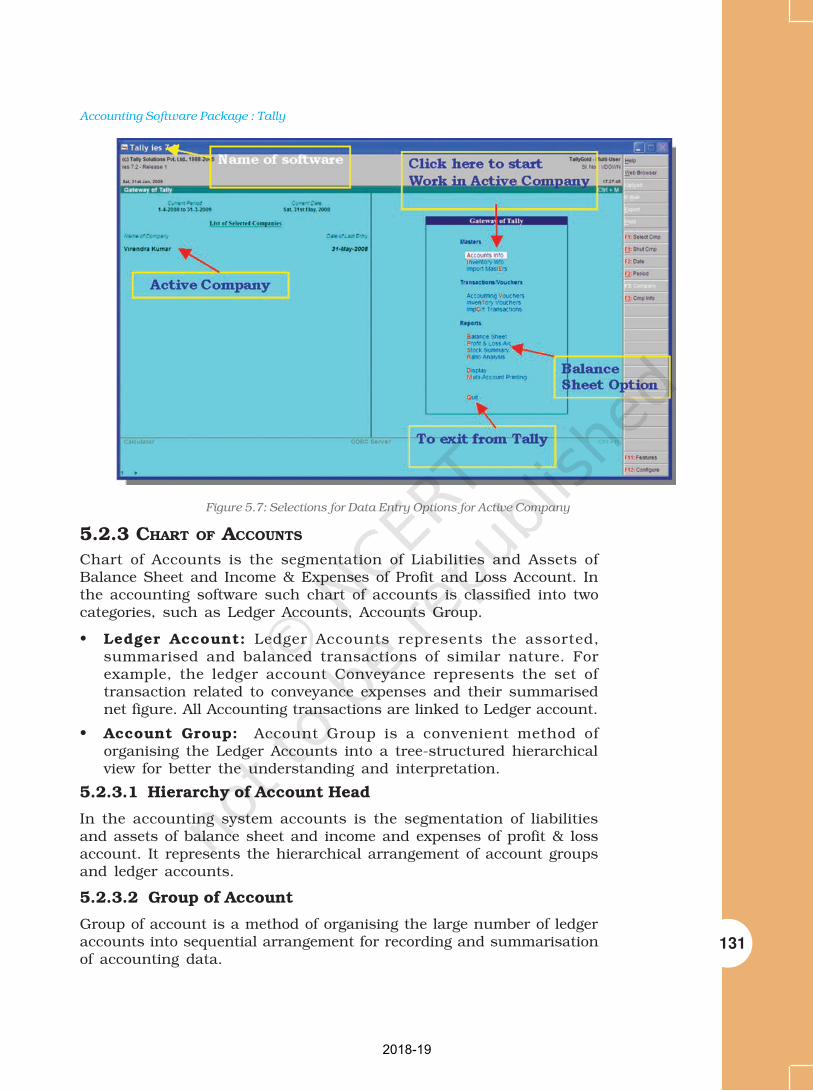
Accounting Software Package : Tally
131
5.2.3 CHART OF ACCOUNTS
Chart of Accounts is the segmentation of Liabilities and Assets ofBalance Sheet and Income & Expenses of Profit and Loss Account. Inthe accounting software such chart of accounts is classified into twocategories, such as Ledger Accounts, Accounts Group.
• Ledger Account: Ledger Accounts represents the assorted,summarised and balanced transactions of similar nature. Forexample, the ledger account Conveyance represents the set oftransaction related to conveyance expenses and their summarisednet figure. All Accounting transactions are linked to Ledger account.
• Account Group: Account Group is a convenient method oforganising the Ledger Accounts into a tree-structured hierarchicalview for better the understanding and interpretation.
5.2.3.1 Hierarchy of Account Head
In the accounting system accounts is the segmentation of liabilitiesand assets of balance sheet and income and expenses of profit & lossaccount. It represents the hierarchical arrangement of account groupsand ledger accounts.
5.2.3.2 Group of Account
Group of account is a method of organising the large number of ledgeraccounts into sequential arrangement for recording and summarisationof accounting data.
Figure 5.7: Selections for Data Entry Options for Active Company
2018-19
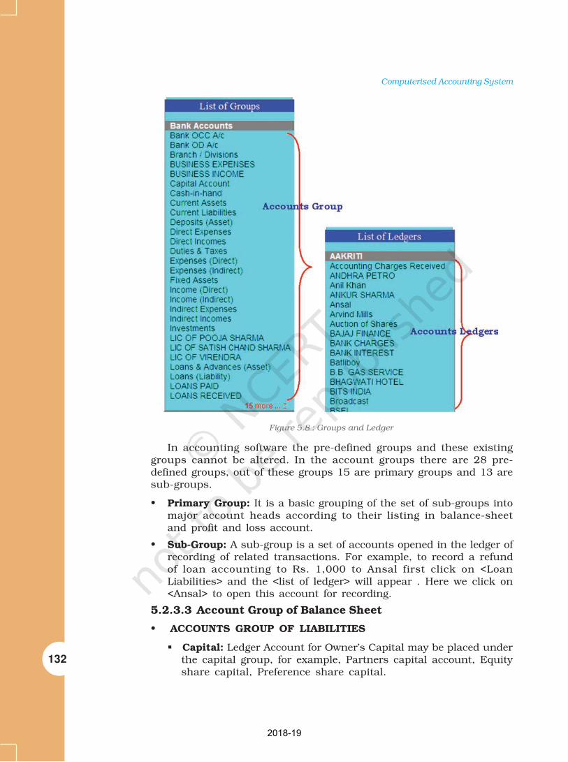
132
Computerised Accounting System
In accounting software the pre-defined groups and these existinggroups cannot be altered. In the account groups there are 28 pre-defined groups, out of these groups 15 are primary groups and 13 aresub-groups.
• Primary Group: It is a basic grouping of the set of sub-groups intomajor account heads according to their listing in balance-sheetand profit and loss account.
• Sub-Group: A sub-group is a set of accounts opened in the ledger ofrecording of related transactions. For example, to record a refundof loan accounting to Rs. 1,000 to Ansal first click on <LoanLiabilities> and the <list of ledger> will appear . Here we click on<Ansal> to open this account for recording.
5.2.3.3 Account Group of Balance Sheet
• ACCOUNTS GROUP OF LIABILITIES
Capital: Ledger Account for Owner’s Capital may be placed underthe capital group, for example, Partners capital account, Equityshare capital, Preference share capital.
Figure 5.8 : Groups and Ledger
2018-19

Accounting Software Package : Tally
133
Reserves and Surplus: It is a sub-group of capital account. Allreserves are placed under Capital group, for example, General.Reserve, Capital Reserve, etc.
• ACCOUNT GROUP – LOANS (LIABILITIES) – It contains followingsub-groups:
Bank Overdraft: In computerized accounting system, CurrentBank Account, Bank Overdraft, and Cash Credit is sub-group ofLoan (Liabilities) because Bank Overdraft and Cash Creditoperation on day-to-day basis should be placed under this group.
Secured Loans: Secured Loan’s are fully secured loan againstsecurity like (mortgage, hypothecation, pledge, etc ) should beplaced under this group .
Unsecured Loans: Such loan’s are without any security: Exampleof such loans are: Loan from outside parties, Directors, Friendsand Relatives, etc.
• ACCOUNTS GROUP – (CURRENT LIABILITIES)
Duties and Taxes: Under this head all duties and taxes thatyou collect or pay through sales service and purchasetransactions.
Provisions: In this head all provisions made for meeting thefuture liabilities such as provision for tax , proposed dividends(like Bad Debts, etc ).
Sundry Creditors: Sundry Creditors are all trade creditors/suppliers and creditors for expenses. For example, if youpurchase, on credit basis then create one ledger account forsundry creditors.
Other Current Liabilities: Place all other current liabilityaccount like employees contribution for Employees StateInsurance/Provident Fund/Tax Deducted at Source (TDS), etc.
• ACCOUNT GROUP OF ASSETS:
ACCOUNTS GROUP (FIXED ASSETS)ACCOUNTS GROUP (FIXED ASSETS)ACCOUNTS GROUP (FIXED ASSETS)ACCOUNTS GROUP (FIXED ASSETS)ACCOUNTS GROUP (FIXED ASSETS)
Fixed assets: Fixed assets directly related with immovableproperties like Patent, Trade Right, W.I.P, Goodwill, Building,Plant, Equipment, Furniture, etc
• ACCOUNTS GROUP (INVESTMENT)
Investment: Investment ledger account relates to the investmentin Share Bonds, Govt. Securities and Investments in other company
• ACCOUNTS GROUP (CURRENT ASSETS): Those assets whichconsumed in operations are known as current assets. Examples ofcurrent assets are Stock on hand, Deposits, Loan and Advances,Sundry Debtors, Bank Account, Cash in hand.
2018-19
134
Computerised Accounting System
Stock on Hand: Such ledger accounts show Raw Material, Work–in-Progress and Finished goods.
Loans and Advances: Such loans and advances are of non-trading nature, for example, Advance against Salary, Loan toemployee, Advance for Fixed Assets.
Sundry Debtors: Sundry Debtors are directly related to the partiesto whom goods has been sold on credit.
Bank Account: It includes bank deposits made by the companysuch as balance of current and saving account, fixed depositssecurity deposits, rental deposits, etc.
Cash in Hand: Cash Ledger account directly relates with cashtransactions, Cash in transit, patty cash, and cash at bank.
Miscellaneous Expenditure: For limited company, preliminary,pre-operative and similar expenses (to the extent not written-offto the profit and loss account placed here. Also the accumulatedloss as of the company and negative balance of profit & lossaccount is also placed in this category.
• PROFIT AND LOSS ACCOUNT
Sales Account: For different sales accounts, the segregation isbased on tax slabs or type of sales. This also becomes a simplemechanism for preparation of tax returns. For example, Salesaccount is classified as following such-groups: domestic sales,export sales, You may even open sales returns account underthe group domestic sales to view net sales after returns (or thereturns may be directly recorded through journal against thespecific sales account).
Purchase Account: This is similar to sales accounts, except forthe purpose of the transaction.
Direct Income [Income Direct] All trade income accounts fallunder sales accounts. You may wish to use this group foraccounts like servicing contract charges that follow after thesales of equipment.
Indirect Income [Income Indirect] These are the miscellaneousnon-sale income accounts, e.g., rent received and interestreceived.
Direct Expenses [Expenses Direct] These accounts determinethe Gross Profit of the company.
Indirect Expenses [Expenses Indirect] - These include all otheradministrative, selling or non-direct expenses.
Tally automatically opens the profit and loss account which is areserved primary account. You may use this account to recordadjustment entries through journal vouchers.e.g., transfer of profitor loss to capital or reserve account.
2018-19

Accounting Software Package : Tally
135
5.2.4 ACCOUNT MASTER
• ACCOUNTS GROUP CREATIONS
Select Accounts info at Tally Main Menu (Figure 5.9) to get <Accountsinfo Menu>, which contains options for all Accounts Masters.
After selecting Create option under Single Group to reach to theAccount Group creation screen. Now enter as shown in Figure 5.10,
Account Group Name: At name field, enter unique AccountGroup Name.
Parent Group Name: At under field, select the Parent Groupfrom list of Group.
Figure 5.9 Account Groups
Figure 5.10 : Account Group
2018-19

136
Computerised Accounting System
• ACCOUNTS LEDGER CREATION: Tally automatically creates twoledgers, one Cash and another Profit and Loss Accounts. You haveto create all other Ledger Accounts (Figure 5.11).
Account Ledger Name: - Enter a unique Name of the ledger
at Under field select the parent Group of the ledger from list ofGroup.
In the Opening Balance field enter the opening balance at theBooks Beginning from Date .
Figure 5.11 : Account Ledger
Figure 5.12 displays the user Account Group and Ledger aftercreation. The next step is the Creation of necessary ledgers. via creationof vouchers.
5.2.5 VOUCHER ENTRY
After creation of accounts the user enters accounting voucher entry inthe books of accounts. In the computerized accounting system, thetransactions are recorded through a voucher entry. Normally, atransaction is supported by a document that may be a supplier’s bill,pay-in-slip, pay register entry of cheque book, etc. Thus, basicallyvoucher contains details of a transaction. In accounting software,Voucher creation displays its own screen which is self-explanatory.The vouchers are three types —:
Memo Voucher: Memo voucher is a non accounting voucher.It does not affect accounts of the user. These entries are stated/recorded in a separate register, but not as a part of ledger.
2018-19

Accounting Software Package : Tally
137
Post Dated voucher: Some accounting software allows the userto enter the voucher for future transactions which are usuallysimilar as the previous once.
User defined Voucher: In accounting software there are 23 pre-defined vouchers. It allows the user to define or create newaccounting or inventory vouchers as per the requirement. In thevoucher entry, entry can be classified into three basic categories.
• Opening Entry: In order to begin the new financial year, balancesof accounts of the previous year are brought forward. For this openingentry in the journal is recorded. It is to record the opening balanceof various accounts that are being transferred from the books of theprevious year to the books of the new financial year. All thoseaccounts which shows the assets of a business are debited and allthe accounts showing amounts owed by the business (liabilities)are credited. If capital amount is not given, it can be easily ascertained by deducting liabilities from assets (capital = assets –other liabilities) and Capital account is also credited. The entrywould be :
• Closing Entry: The closing entries for completing the profit andloss account are :
1. Debit Profit and Loss account.Credit the various Expenses account appearing in the TrailBalance.
2. Debit account showing incomes or gains
Credit the profit and loss account
This will close the profit and loss account. Entries required to makethe trading account and profit and loss account are known as closingentries because their effect is to close the books of account for the yearconcerned.
Cash account Dr
Cash at Bank account Dr
Sundry Debtors account Dr
Stock account Dr
Furniture account Dr
Office Equipment account Dr
To Sundry Creditors account
To Capital account
2018-19

138
Computerised Accounting System
• Adjusting Entry: The Adjusting entry is recorded to relate thefigures to the trading period. Suppose, premises have been subleton March 31, and three months’ rent, has been received in advanceamounting to Rs. 9000. While preparing accounts up to 31st March,one should take into account only one month’s rent for preparingthe profit and loss account (accounting period concept); the resttwo month’s rent, already received is for the next year and will becredited to profit and loss account next year. The adjusting entrywill be :
Rent Account Dr.
To Advance Rent Account
Rent Received in advance Account is a ‘Liability’ and is shown inthe balance sheet.
Method of Voucher Numbering: This is, perhaps, one reason foryour opting for a new voucher type. For this purpose, the followingmedhods are available:,
• Manual
This method will allow you to number vouchers yourself. Howeverit does not check for sequence of the numbers and permits you tospecify anything you wish in the voucher number field. However,you may choose to prevent entry of duplicate numbers. If you do,enable the next field ‘Prevent Duplicates’ — options Prevention ofDuplicates is possible if you enable the option at the time of creation.You may enable it later (by alteration) only if there are notransactions of this voucher type.
• Automatic
This method is both; flexible and exhaustive. Automatic systeminstructs Tally to number the vouchers of this type incrementingautomatically.
Starting number
Give the number for the first voucher. Usually it is 1. You can set it toany number you want. Tally will auto-increment from this number forsubsequent vouchers. However, the numbering of vouchers also dependson other variables supplied by you, which follow hereafter.
In the voucher entry, Tally create certain rules to trap mistakes.These rules are validated during voucher entry and any violation istrapped immediately. Tally divides a voucher in three basic categories,
• Contra Voucher: Contra voucher is used for Fund Transfer betweenCash and Bank account only. For example, Rs 5,000 Cash withdrawnfrom Bank of India .
Cash A/C Dr 5,000.00
To Bank of India 5,000.00
(Cash withdrawn from bank )
2018-19

Accounting Software Package : Tally
139
• Receipts Voucher :- All Inflow of money is recorded through ReceiptVoucher. Such receipts may be towards any Income such as receiptsfrom debtors, loan/advance taken or refund of loan/advance forexample: Rama and Co. to whom goods were sold earlier on Credit,paid against Bill No 54 for Rs 4,500 Cash Discount is Rs 500.
Cash A/C Dr. 4,500.00
Cash Discount A/C Dr. 500.00
To Rama & Co. Cr. 5,000.00
(Cash Payment Received against Bill no 54)
• Payment Voucher: All Outflow of money is recorded throughPayment Voucher. Such payment may be towards any purchase,Expenses, due to creditors, loan/advances, etc. For example: - Salarypaid to A.K Gupta through Bank.
Salary A/C Dr 15,000.00
To Bank Cr 15,000.00
(Salary Paid to Mr A.K Gupta through Bank)
• Journal Voucher: Journal is an Adjustment voucher, normally usedfor non cash transaction like adjustment between the Ledgers. Forexample :-
Deprecation A/C Dr 5,000.00
To Machinery 5,000.00
(Being Deprecation charged on Machinery)
Display: Some top level reports like Balance Sheet, Profit and LossAccount etc may be available at main menu, while other reports areavailable through Display option at main menu .
Figure 5.12 Voucher Entry
2018-19

140
Computerised Accounting System
5.2.6 TRIAL BALANCE
This report shows the trial balance of a Primary Group.
Select Display > Trial Balance.
In Primary Group trial balance (Figure 5.13), Click F1: obtain detailtrial balance and trial balance shows the closing balance of accountsgroup/Ledger. After all voucher entry have been done, it can be seenhow every amount that is placed on the debit side of an account has acorresponding entry on the credit side of some other account. This isthe technical aspect of the principle of double system. This being thecase, that the total of the debit balances hold agree with the total of allthe credit balances. In fact all businesses periodically tabulate thedebit and credit balances separately in a statement to find out whetherthe total of debit balances agree with the total of credit balances ornot. Such a statement is known as the trial balance.
5.2.7 BALANCE SHEET AND PROFIT AND LOSS ACCOUNT
The Profit and Loss account is constructed by simply posting all itemsof income and expense from the journal entry. The current year’s profitis determined by balancing the accounts and carried forward to theappropriation section of the profit and loss account. All balancesremaining in any ledger account after the profit and loss account isdrawn up are listed in the balance sheet .Generally the assets andliabilities are stated in decreasing order of permanence.
All expenses (direct or indirect) are related to profit and loss accountand revenues and incomes are credited to it. If an expense has beenincurred but not yet paid for, is a liability for the unpaid amount andmust be created before the account can be said to show a true picture.
Figure 5.13 : Trial Balance
2018-19

Accounting Software Package : Tally
141
BALANCE SHEET OF M/S XYZ LTD AS ON 31-03-2009
Figure 5.14 : Balance Sheet
Description Amount Description Amount
Share Capital Fixed assets
Authorised Capital Goodwill
Paid up Capital Land and Building
Reserve and Surplus Plant and Machinery
Capital Reserve Furniture and Fixture
Other Surplus Investment
Secured Loans Govt securities
Debentures Share Bond and Debenture
Loans from Bank Current Assets
Other Loans Loan and Advances
Unsecured Loans Sundry Debtors
Fixed Deposits Cash and Bank
Advances from Bank Stock in Trade
Other Loans Accrued Interest
Current Liabilities Loan and Advances
Sundry Creditors Bill of Exchange
Advances from Bank Miscellaneous Expenditure
2018-19

142
Computerised Accounting System
Provision for Tax Commission on Underwriting
Provision for P. dividend Discount on Share
Other Provision Development Expenditure
Profit and Loss Account (loss)
Total Liabilities Total Assets
5.2.8 DISPLAY OF REPORT
Once all the transactions are entered, you can generate differentstatements like trial balance, balance sheet and profit and loss account.There are no intermediate steps of entering subsidiary books andledgers. Thus the process of accounting becomes quite easy and simple.At the same time speed also improves and consistency is maintained.Also no redundant data is stored at multiple places. Also the respectiveregister such as purchase register, sales register, journal proper areautomatically maintained on the basis of data entered in the form ofvouchers. These registered can be viewed by
• Selecting Gateway of Tally > Report >Display>Accounts Books >Sales
register.
• Selecting Gateway of Tally > Report >Display>Trial Balance.
• Selecting Gateway of Tally > Report >Display>Cash flow.
• Pressing Alt + P or selecting print option for button bar
5.2.9 A SMALL PROJECT WITH BANK RECONCILIATION
STATEMENT (BRS)
The following are the steps to construct BRS in Tally:
• Bring up the monthly summary of any Bank Book. (You can do thisfrom the Balance Sheet, Trial Balance, or Display/Account Books/Bank Books, and selecting a Bank).
• Bring your cursor to the first month (typically April), and pressEnter. This brings up the Vouchers for the month of April. Sincethis is a Bank Account, an ‘additional’ button F5: Reconcile will bevisible on the right, Press F5.
• The display now becomes an ‘Edit’ screen in ‘Reconciliation’ mode.The primary components are: A column for the ‘Bankers Date’.
• The ‘Reconciliation’ at the bottom of the screen,
• Balance as per Company Books
• Amounts not reflected in Banks
• Balance as per Bank
2018-19

Accounting Software Package : Tally
143
Gateway of Tally>Display>Accounts Books>Cash and Bank
Book>Bank Account>Ledger>Press F5
The Balance as per Company Books reflects your Balance as on thelast date (in our example case, April 31).
The amount not reflected in bank is the debit and credit sums of allthose vouchers whose Bank Date in either BLANK, or GREATER thatApril 30 (i.e. these vouchers have not yet been reflected in the bankStatement).
The Balance as per bank is the Net Balance.
You will find, as you mark of the individual vouchers by setting the‘Bank Date’, that the Reconciliation at the bottom of screen keepsreflecting those changes instantly.
Upon completion, press+A (or press Enter as many times as necessaryto skip over the unmarked vouchers), and accepted the screen. Thenext time you reconcile, you will be presented only with those voucherswith remain unrecognised. Thus, the task keeps becoming simpler.
5.3 NEED AND SECURITY FEATURE OF THESYSTEM
Every accounting software provides data security; safety andconfidentially; so every software provides of data security in three ways:
• Password security
• Data Audit
• Data Vault
Figure 4.15 : Bank Reconciliation Statement
Particular of
Payment/receipt
Mention the date
of Cheque cleared
Debit/Credit
amount
2018-19

144
Computerised Accounting System
Password Security Password is widely accepted security control toaccess the data. Only the authorised person can access the data. Anyuser who does not know the password cannot retrive information fromthe system. It ensures data integrity. It uses a binary encoding formatof storage and offers access to the database.
Data Audit: Audit feature of accounting software provides the userwith administrator right in order to keep track of unauthorised access.to the database. It audit for the correctness of entries. Once entriesare audited with alternations, if any the software displays all entriesalong with the name of the auditor user and date and time of alteration.
Data Vault: Software provides additional security for the inputeddata and this feature is referred as data vault. Data vault ensuresthat original information is presented and is not tampered. Data vaultpassword cannot be broken. Some software uses data encryptionmethod.
Function Key CombinationFunction Key CombinationFunction Key CombinationFunction Key CombinationFunction Key Combination
Windows Functionality Availability
F1 To select a company At all masters menu screen
To select the Accounts Button At the Accounting/Inventoryand Inventory buttons Voucher creation and
alteration screen
F2 To change the menu period At almost all screens in TALLY
F3 To select the company At almost all screens in TALLY
F4 To select the Contra voucher At Accounting/InventoryVoucher creation and alterationscreen
F5 To select the Payment voucher At Accounting/InventoryVoucher creation and alterationscreen
F6 To select the Receipt voucher At Accounting/InventoryVoucher creation and alterationscreen
F7 To select the Journal voucher At Accounting/Inventory Voucher creation and alteration screen
F8 To select the Sales voucher At Accounting/Inventory Vouchercreation and alteration screen
F8 To select the Credit Note voucher At Accounting/Inventory Voucher(CTRL+F8) ercreation and alteration screen
F9 To select the Purchase voucher At Accounting/Inventory Vouchercreation and alteration screen
F9 To select the Debit Note voucher At Accounting/Inventory Voucher(CTRL+F9) creation and alteration screen
2018-19

Accounting Software Package : Tally
145
F10 To select the Reversing Journal At Accounting/Inventory Vouchervoucher creation and alteration screen
F10 To select the Memorandum voucher At Accounting/Inventory Vouchercreation and alteration screen
F11 To select the Functions and Features At almost all screens in TALLYscreen
F12 To select the Configure screen At almost all screens in TALLY
Special Key CombinationSpecial Key CombinationSpecial Key CombinationSpecial Key CombinationSpecial Key Combination
Windows Functionality Availability
ALT + 2 To Duplicate a voucher. At List of Vouchers – creates a vouchersimilar to the one where you positionedthe cursor and used this keycombination.
ALT + A To Add a voucher. At List of Vouchers – adds a voucherafter the one where you positionedthe cursor and used this keycombination.
ALT + C To create a master at a voucher At voucher entry and alterationscreen (if it has not been already screens, at a field where you have toassigned a different function, as in select a master from a list. If thereports like Balance Sheet, where it necessary account has not beenadds a new column to the report). created already, use this key
combination to create the masterwithout quitting from the voucherscreen.
ALT + D To delete a voucher. At Voucher and Master (Single)To delete a master. alteration screens. Masters can be(if it has not been already assigned deleted subject to conditions, asa different function, as explained above). explained in the manual.
ALT + E To export the report in ASCII, SDF, At all reports screens in TALLY.HTML OR XML format.
ALT + I To insert a voucher. At List of Vouchers – inserts a voucherbefore the one where you positioned thecursor and used this key combination.
ALT + O To upload the report at your website. At all reports screens in TALLY.
ALT + M To Email the report. At all reports screens in TALLY.
ALT + P To print the report. At all reports screens in TALLY.
ALT + R To remove a line in a report. At all reports screens in TALLY.
ALT + S To bring back a line you removed At all reports screens in TALLY.
using ALT + R.
ALT+ V From Invoice screen to bring At Invoice screen/Quantity Field/
Stock Journal screen. Press Alt + V to select the Stock Journal.
2018-19

146
Computerised Accounting System
Windows Functionality Availability
ALT + W To view the Tally Web browser. At all reports screens in TALLY.
ALT + X To cancel a voucher in Day Book/ At all voucher screens in TALLY.
List of Vouchers.
ALT + R To Register Tally. At Licensing Menu in TALLY.
CTRL + A To accept a form – wherever you use At almost all screens in TALLY, except
this key combination, that screen or where a specific detail has to be given
report gets accepted as it is. before accepting.
CTRL + B To select the Budget. At Groups/Ledgers/Cost Centres/
Budgets/Scenarios/Voucher Types/
Currencies (Accounts Info) creation and
alteration screen.
CTRL + C To select the Cost Centre. At Groups/Ledgers/Cost Centres/
Budgets/Scenarios/Voucher Types/
Currencies (Accounts Info) creation and
alteration screen.
To select the Cost Category. At Stock Groups/ Stock Categories/
Stock Items/ Reorder Levels/ Godowns/
Voucher Types / Units of Measure
(Inventory Info) creation/alteration
screen.
CTRL+ E To select the Currency. At Groups/Ledgers/Cost Centres/
Budgets/Scenarios/Voucher Types/
Currencies (Accounts Info) creation and
alteration screen.
CTRL + G To select the Group. At Groups/Ledgers/Cost Centres/
Budgets/Scenarios/Voucher Types/
Currencies (Accounts Info) creation and
alteration screen.
CTRL + I To select the Stock Items. At Stock Group/ Stock Categories/ Stock
Items/ Reorder Levels/ Godowns/
Voucher Types / Units of Measure
(Inventory Info) creation/alteration
screen.
CTRL + L To select the Ledger. At Groups/Ledgers/Cost Centres/Budgets/Scenarios/Voucher Types/Currencies (Accounts Info) creation andalteration screen.
CTRL + O To select the Godowns. At Stock Group/ Stock Categories/ StockItems/ Reorder Levels/ Godowns/Voucher Types / Units of Measure(Inventory Info) creation/alterationscreen.
2018-19

Accounting Software Package : Tally
147
Windows Functionality Availability
CTRL + Q To abandon a form – wherever you At almost all screens in TALLY.use this key combination, it quits thatscreen without making anychanges to it.
CTRL+Alt+R Rewrite data for a Company. From Gateway of Tally screen.
CTRL + S Allows you to alter Stock Item master. At Stock Voucher Report and GodownVoucher Report.
CTRL + U To select the Units. At Stock Groups/Stock Categories/Stock Items/Reorder Levels/Godowns/Voucher Types/Units of Measure(Inventory Info) creation/alterationscreen.
Ctrl + V To select the Voucher Types. At Groups/Ledgers/Cost Centres/Budgets/Scenarios/Voucher Types/Currencies (Accounts Info) creation andalteration screen. Special Function KeyCombination
Special Key CombinationSpecial Key CombinationSpecial Key CombinationSpecial Key CombinationSpecial Key Combination
Windows Functionality Availability
ALT + F1 To close a company. At all the menu screen.To explode a line into its details. At almost all report screen.To view detailed report. At almost all screens in TALLY.
ALT+ F2 To change the system period. At almost all screens in TALLY.
ALT + F3 To select the company info menu. To create/alter/shut a Company.At Gateway of Tally screen.
ALT + F4 To select the Purchase Order At Accounting/InventoryVoucher Type. Voucher creation and alteration screen.
ALT + F5 To select the Sales Order At Accounting/Inventory VoucherVoucher Type. creation and alteration screen.
To view monthly and quarterly At almost all report screens inreport. TALLY.
ALT + F6 To select the Rejection At Accounting/Inventory Voucher
Out Voucher Type. creation and alteration screen.
To change the Sales Order
Voucher Type.
ALT + F7 To select the Stock Journal At Accounting/Inventory Voucher
Voucher Type creation and alteration screen.
To accept all the Audit lists At TallyAudit Listing screen
ALT+ F8 To select the Delivery Note At Accounting/Inventory Voucher
Voucher Type. creation and alteration screen.
To view the Columnar report. At Ledger Voucher screen.
2018-19
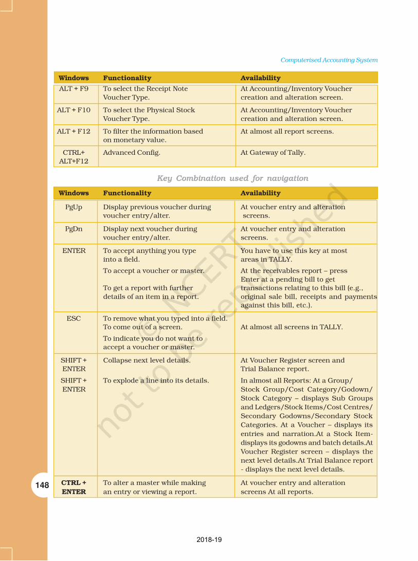
148
Computerised Accounting System
Windows Functionality Availability
ALT + F9 To select the Receipt Note At Accounting/Inventory Voucher
Voucher Type. creation and alteration screen.
ALT + F10 To select the Physical Stock At Accounting/Inventory Voucher
Voucher Type. creation and alteration screen.
ALT + F12 To filter the information based At almost all report screens.
on monetary value.
CTRL+ Advanced Config. At Gateway of Tally.
ALT+F12
Key Combination used for navigationKey Combination used for navigationKey Combination used for navigationKey Combination used for navigationKey Combination used for navigation
Windows Functionality Availability
PgUp Display previous voucher during At voucher entry and alteration
voucher entry/alter. screens.
PgDn Display next voucher during At voucher entry and alteration
voucher entry/alter. screens.
ENTER To accept anything you type You have to use this key at most
into a field. areas in TALLY.
To accept a voucher or master. At the receivables report – press
Enter at a pending bill to get
To get a report with further transactions relating to this bill (e.g.,
details of an item in a report. original sale bill, receipts and payments
against this bill, etc.).
ESC To remove what you typed into a field.
To come out of a screen. At almost all screens in TALLY.
To indicate you do not want to
accept a voucher or master.
SHIFT + Collapse next level details. At Voucher Register screen and
ENTER Trial Balance report.
SHIFT + To explode a line into its details. In almost all Reports: At a Group/
ENTER Stock Group/Cost Category/Godown/
Stock Category – displays Sub Groups
and Ledgers/Stock Items/Cost Centres/
Secondary Godowns/Secondary Stock
Categories. At a Voucher – displays its
entries and narration.At a Stock Item-
displays its godowns and batch details.At
Voucher Register screen – displays the
next level details.At Trial Balance report
- displays the next level details.
CTRL + To alter a master while making At voucher entry and alteration
ENTER an entry or viewing a report. screens At all reports.
2018-19

Accounting Software Package : Tally
149
SummarySummarySummarySummarySummary
• In computerised accounting system, accounting transactions are journalised
by two methods (1) manually (2) computerised. In the present computerized
accounting system are more and more effective in comparison of manual
system of accounting. There are different type of accounting softwares in
market but Tally 9.0 is more effective accounting software. Tally 9.0 software
have a different features these are :
i) Gateway - Gateway is the starting of Tally. In other words we can say
that gateway is the gate to enter in Tally.
ii) Company creation - Before inputing accounting transactions, first we
create a company through company creation.
iii) Chat of accounts - Chart of accounts is the segmentation of Liabilities
and Assets of Balance Sheet and preparation of Profit and Loss account.
iv) Account master - Account master basically used for account group
and ledger .
v) Voucher entry - After creation of account user inputs accounting
voucher entry in the book of accounts. In computerised accounting
system all entries are inputed through a voucher entry.
vi) Trial Balance - Trial balance is the statement of different closing
balances of ledger.
vii) Balance Sheet - The balance sheet is constructed by simply posting all
items of liabilities and assets for the finalisation of journal entry.
• Report printing - Report printing is the last step of accounting process.
• Accounting software can be used to successfully maintain the financial
transactions of any organisation. Besides data maintenance, these prove to
be very efficient when we have to generate accounting reports, which are
crucial for decision making in an organisation. These software packages
have many more features, which can be explored and used depending on
the type of transaction details you require.
2018-19

150
Computerised Accounting System
EXERCISE
Q. 1. MULTIPLE CHOICE QUESTIONS
A. To create group which menu is used?
a. Gateway of Tally > master >accounts info > create
b. Gateway of Tally > master >accounts info > alter
c. Gateway of Tally > master >accounts info > display
d. Gateway of Tally > master >accounts info > edit
B. To create ledger which menu is used ?
a. Gateway of Tally > master >accounts info >ledger > create
b. Gateway of Tally > master >accounts info > ledger >alter
c. Gateway of Tally > master >accounts info > ledger >display
d. Gateway of Tally > master >accounts info > ledger>edit
C. Which short cut is used to shift “company information menu” form gateway ofTally?
a. Alt + F3
b. Alt + Escape
c. Shift + F3
d. Shift + F1
D. In which group will you record the expense of light bill of Factory?
a. Direct income
b. Direct Expense
c. Indirect income
d. Indirect Expense
E. While recording the voucher entry if it is necessary to create a new ledger for
that which commands is used in Tally?
a. Ctrl + C
b. Ctrl + G
c. Alt + C
d. Alt + G
F. While creating ledger if you want to create new group which key is pressed?
a. Ctrl + C
b. Ctrl + G
2018-19

Accounting Software Package : Tally
151
c. Alt + C
d. Alt + G
G. ……………… works as a platform to work with Tally
a. Gateway of Tally
b. Outway of Tally
c. Company information
d. All the above
H. How many characters are used to create company’s short name?
a. 2
b. 4
c. 3
d. 5
Q. 2. ANSWER THE FOLLOWING QUESTIONS
1. How do you begin using Tally accounting software?
2. What menu option is available on the gateway of Tally screen?
3. What is the use of Button bar in Tally accounting package?
4. What are the contents of Balance Sheet in Tally?
5. What do you mean by Account Info?
6. Explain the process of Company Creation?
7. “Report generating is not a easy task” Is this statement true or false Explain?
8. Describe the various contents of Profit and Loss Account?
9. Describe the process of creating a Group company and how would you Displayand Alter a Group account?
10. Describe Tally 9.0 and what are the new features of 9.0, and explain the variousitems of the Tally screen?
Q. 3. SKILL REVIEW
1. From the following transactions of Ashirwad Ltd, post the voucher entries in
the respective ledger accounts, prepare a trial balance and balance sheet.
i. Started a business with cash Rs 40,000
ii. Goods of Rs 10,000/- were purchased at 10% trade discount
iii. Goods of Rs 5,000/- were sold with a profit of 40% to Arjun
iv. Commission received Rs 500
v. Cash deposited Rs 7,000 in a bank
2018-19

152
Computerised Accounting System
vi. Return of goods Rs 1,500
vii. Salary paid Rs 2,500
viii. Wages paid Rs 350
ANSWERS
1. a 2. a 3. a 4. d 5. c 6. b
7. a 8. b
2018-19
DATA BASE
MANAGEMENT SYSTEM
FOR ACCOUNTING
IntroductionAfter studying this unit you will be able
to:
• Understand how to Structure
database as per requirement.
Design and create database
tables.
• Make use of Microsoft Access for
simple database applications
involving creation of back-end
database and the front-end
forms for capturing, processing
and retrieval of data.
6
One of the major factors for realising the need ofComputerised Accounting System is theoverwhelming quantity of data in ourorganisations. The conventionally used paper filingsystem, text documents, and even spread-sheetsmay not suffice for the growing needs of trackingthis voluminous and critical information. A simplesolution to this situation is available in the formof a Database Management System (DBMS) (e.g.‘Access’, ‘Oracle’, ‘SQL Server’, etc.) that providesa variety of software tools for organising,processing and querying data in a flexible manner.
As we now proceed to look into practicalapplications of computers in generating, storing,processing, and retrieving of accountinginformation, we will make an assumption that youare fairly conversant with the accounting frameworkand operating procedure – i.e. you have the requireddomain knowledge. We also assume that you haveadequate exposure to handling of computers andthe concepts of database. However, we do not wishto make knowledge of the database management apre-requisite for understanding of this chapter,and hence, we will restrict ourselves to the simplerand easy to comprehend ‘MS Access’ program fordeveloping some practical accounting applications.In doing so, we will focus on the three majorcomponents of Access, namely, ‘tables’, ‘queries’and ‘forms’. Having done that, we will examinethe methods of generating reports. This basicallybuilds on the concepts of DBMS already learnt byyou in class XI.
2018-19
154
Computerised Accounting System
8.1 UNDERSTANDING AND DEFINING THEDATABASE REQUIREMENT
With the continuous improvements in computer’s processing speed,storage capacity, networking techniques, operating systems, etc, thecapabilities of computer applications have also gone up many folds.Various computer applications that are commercially available todaynot only provide fairly comprehensive tools for all conceivable needsbut also have become extensively user friendly. So, when we lookforward to putting into use database applications such as ‘Access’, wereally do not need much of programming skills. Nevertheless, anyprogramming knowledge may improve our efficiency and effectivenessin handling such applications. On the other hand, before we developany database application, we ought to have a complete understandingof our requirements expected from the application. This is one areawhere application itself may not extend much help. Further, the correctunderstanding of our requirement also has a bearing on the choice ofDatabase Management Systems (DBMS) - i.e. whether to go for a ‘desktopdatabase’ or to choose the ‘server database’.
Box - 6.1Box - 6.1Box - 6.1Box - 6.1Box - 6.1
In most of the cases, database is not directly accessible to users. Any
addition, modification or retrieval of information from database is done
by the user-friendly programs. Database is thus rightly referred to as
‘back-endback-endback-endback-endback-end’ while the interactive program is termed as ‘frfrfrfrfront-endont-endont-endont-endont-end’ of a
database application.
While the desktop databases – residing on standard personal computers– are oriented toward single-user applications, ‘server databases’ aregeared toward multi-user applications. Understandably the ‘serverdatabase’, containing additional provisions for ensuring reliability andconsistency of data in a multi-user environment, are substantially costlierthan the ‘desktop database’. Hence, it is imperative to do a carefulanalysis of our requirements before investing in a database solution.Some of the questions that need to be answered in this regard are:
• What all data is required to be stored in the database?
• Who will capture or modify the data, and how frequently the datawill be modified?
• Who all will be using the database, and what all tasks will theyperform?
• Will the database (backend) be used by any other front-endapplication?
• Will access to database be given over LAN (Local Area Network)/Internet, and for what purposes?
• What level of hardware and operating system is available?
6.1 UNDERSTANDING AND DEFINING THEDATABASE REQUIREMENT
With the continuous improvements in computer’s processing speed,storage capacity, networking techniques, operating systems, etc, thecapabilities of computer applications have also gone up many folds.Various computer applications that are commercially available todaynot only provide fairly comprehensive tools for all conceivable needsbut also have become extensively user friendly. So, when we lookforward to putting into use database applications such as ‘Access’, wereally do not need much of programming skills. Nevertheless, anyprogramming knowledge may improve our efficiency and effectivenessin handling such applications. On the other hand, before we developany database application, we ought to have a complete understandingof our requirements expected from the application. This is one areawhere application itself may not extend much help. Further, the correctunderstanding of our requirement also has a bearing on the choice ofDatabase Management Systems (DBMS) - i.e. whether to go for a ‘desktopdatabase’ or to choose the ‘server database’.
2018-19

Database Management System for Accounting
155
If our requirement entails approach to database by many users, or if itinvolves simultaneous updating of data by different users, then perhapsserver databases such as ‘Microsoft SQL Server’, ‘Oracle’ or ‘IBM DB2’will provide desired solutions.
Although carrying high price tags, a server-based database cangive you several advantages in terms of flexibility for the choice offront-end applications, powerful performance independent of platform,and scalability to handle rapidly expanding number of users as well asamount of data.
Box - 6.2Box - 6.2Box - 6.2Box - 6.2Box - 6.2
Quite often, same database is required to be used by different
applications. For example, an organisation may have automated
attendance recording system which will record the arrival and
departure time of employees. A variety of such systems (e.g. Card-
swipe, Biometric, etc.) are available in the market, and all of them
come with their own (back-end) database and requisite (front-end)
programs. This attendance information may be required for generating
salary bills of the employees. The payroll application of the organisation,
with its own (back-end)(back-end)(back-end)(back-end)(back-end) database and (front-end)(front-end)(front-end)(front-end)(front-end) program, will also
access the database of attendance recording application.
Box - 6.3Box - 6.3Box - 6.3Box - 6.3Box - 6.3
Access 2007 usually comes as part of Microsoft Office 2007. However,
it can also be purchased separately as a standalone program. In order
to run this program, your computer should have a minimum configuration
of 500 MHz Processor, 256 megabyte RAM, 1.5 gigabyte Hard disk,
and Windows XP Operating system.
Comparatively, the desktop databases offer an inexpensive and simplesolution to many of our business data storage and processingrequirements. The ‘Microsoft Access’ is one such database - whichcomes with the licensed copy of Microsoft Office Professional – providingone of the simplest and most flexible DBMS solutions today, besidesgiving the advantages of familiar ‘Windows’ look and integration withother Microsoft Office products such as ‘Excel’.
Before opting for any of the database management system, it will benecessary to ensure that your hardware as well as operating systemmeets the minimum system requirements of the desired DBMS. Asstated earlier, we will be enumerating examples of ‘Access’ applications,and hence it is imperative that your computer lab is equipped with thelicensed copy of ‘MS Access’ with compatible configuration of thehardware. The illustrations contained in this book are based on Access-2007, which may feel a little different from what you are working within case your application is of a different version.
2018-19

156
Computerised Accounting System
Even on same version of the ‘Access’, marginal differences mayappear in the illustrated diagrams and the views on your computerand this may happen on account of variations in the customised settingsof the application. However, these variations are not expected to hamperyour understanding of the contents of this chapter.
6.2 IDENTIFICATION OF DATA TO BE STORED INTABLES
By now we understand that a database is simply an organised collectionof data with ‘tables’ as its fundamental building blocks. Tables allowus to create the framework for storing information in the database.Each column (also called ‘field’) of the table corresponds to a specificcharacteristic (or ‘attribute’ in database terms) of the storedinformation. Each row (also called ‘record’) corresponds to a particularinstance of the information.
Box - 6.4Box - 6.4Box - 6.4Box - 6.4Box - 6.4
In Access 2007, the entire database is encompassed in a file (with
extension .accdb) which can be stored in your hard-drive or CD. There
can be multiple tables (each storing a specific set of data) with in this
file. Then there are multiple fields in each table according to different
categories (types) of data within the table. And at every instance
(occurrence) of a collection of data covering all fields, a row/record
gets created.
Box - 6.5Box - 6.5Box - 6.5Box - 6.5Box - 6.5
Identification of various attributes of a database is generally considered
as part of requirement analysis. requirement analysis. requirement analysis. requirement analysis. requirement analysis. Such a process may entail database
designer to elicit needed information from those with the domain
knowledge.
We may get a better understanding of database design by referringto practical example of an accounting problem. We may take up thecase of payroll accounting, concepts of which have already been examinedwhile studying spreadsheet applications in the earlier chapter(referchapter 3). You have already seen how different employees drawdifferent amounts of pay based on the nature and levels of theiremployment, even while subjected to a definite pattern of ‘pay rules’prevalent in the organisation. Since pay rules vary widely fromorganisations to organisations, the database design for them will also
A set of tables often with well established relationships betweenthem constitutes the database covering total spectrum of storedinformation. The term ‘database design’ can be used to describe thestructure of different parts of the overall database.
2018-19

Database Management System for Accounting
157
differ considerably. For our illustration in this chapter, we will considerthe simplified pay pattern for an assumed organisation XYZ Pvt. Ltd.
Let us begin by identifying various attributes of information thatare required to be stored in our Payroll database. We may have a set ofattributes pertaining to employee’s personal details such as: ‘EmployeeID’, ‘Name’, ‘Designation’, and ‘Location’. On the other hand we mayalso deal with such attributes pertaining to employee’s pay as: ‘BasicPay’, ‘Dearness Allowance (DA)’, ‘House Rent Allowance (HRA)’,‘Transport Allowance (TA)’, ‘Provident Fund (PF) Deduction’, etc. Wemay also want to know the attributes of ‘Gross Salary’ and ‘Net Salary’which is obtained by subtracting ‘PF Deductions’ from ‘Gross Salary’.However, ‘Gross Salary’ and ‘Net Salary’ attributes may not requirebeing stored in the database as they are merely computational outcomesfrom other attributes. We may also require some attributes concerningpay formulations such as ‘% Rate of DA’ which may fluctuate month tomonth, ‘% Rate of HRA’ varying with the location of employee, and ‘TASlabs’ varying with the designation of employee.
Box - 6.6Box - 6.6Box - 6.6Box - 6.6Box - 6.6
At this stage you may like to know the limitations of ‘Excel’ in payroll
accounting. If you look back at payroll example in Excel spreadsheet,
you will notice that you have created pay information of a set of
employees for a particular month. For generating information concerning
next month, you will have to change employee specific data such as
‘Actual Basic Pay’, ‘days of attendance’, etc in respective cells.
However, the moment you do this, the information of previous month
will be lost. Understandably, ‘Excel’ is merely providing a template for
certain calculations concerning salaries, and storing single (monthly)
instance of the derived information. Excel eliminates redundant data
and hence multiple instances of information cannot be stored in a
single Excel sheet. You may avoid this situation by effecting changes
in a different copy of the sheet. In this manner you are creating different
spread sheet for different months. This is a cumbersome task, and
furthermore the information in such a case will not be residing in a
single table, or a set of related tables, from where it may be retrieved
for generation of ‘annual income’ or ‘income tax’ information.
Now the main question is how to store these attributes in ourdatabase tables. Shall we make all of above attributes as part of onetable, or shall we opt for multiple tables. The ‘Access’ as such will notput any constraint on the number of tables we opt for, or the type ofdata we chose to put in any table. It will have to be entirely our decision,based on logical structuring of data that we seek to apply. You mayalso apreciate the fact that the purpose of a database is not so muchfor the storage of information, as for its quick retrieval. Hence, youought to structure your database in such a manner that it can bequeried quickly and efficiently.
2018-19

158
Computerised Accounting System
6.3 LOGICAL STRUCTURING OF DATA IN TABLES
Suppose, we seek the simplest structure of a single table containingall attributes listed above. The rows of this table (see Figure-6.1) willcontain both employee’s personal details as well as employee’s paydetails for every instance of the salary drawn by him or her. Since, theinformation will be generated on monthly basis, multiple records willbe created for each employee in the table. Understandably for anyparticular employee, we may expect variations in the pay attributesrecorded under different rows - i.e. different pay components and theresulting gross/net salary may vary from month to month. However,we do not expect monthly variations in the personal attributes of thesame person under different rows. Evidently thus, the structure ofsingle table may not be an efficient one as it will entail unwarrantedrecording of the same personal data multiple times.
MonthMonthMonthMonthMonth EmpEmpEmpEmpEmp Desig.Desig.Desig.Desig.Desig. Locat.Locat.Locat.Locat.Locat. %DA%DA%DA%DA%DA %HRA%HRA%HRA%HRA%HRA BasicBasicBasicBasicBasic DADADADADA HRAHRAHRAHRAHRA TTTTTAAAAA GrossGrossGrossGrossGross PFPFPFPFPF NetNetNetNetNet
& Y& Y& Y& Y& Yearearearearear NameNameNameNameName RateRateRateRateRate RateRateRateRateRate SalarySalarySalarySalarySalary Ded.Ded.Ded.Ded.Ded. SalarySalarySalarySalarySalary
Nov. Ram Chief Delhi 26 30 25000 6500 7500 7000 46000 5000 410002007 Kishore Manager
Nov. Kishan Manager Faridabad 26 20 22000 5720 4400 5000 37120 3000 341202007 Sharma
Nov. Rupali Senior Meerut 26 15 20000 5200 3000 3500 31700 2000 297002007 Varma Engineer
Nov. Surjeet Engineer Meerut 26 15 16000 4160 2400 3500 26060 2000 240602007 Singh
Dec. Ram Chief Delhi 26 30 25000 6500 7500 7000 46000 7000 390002007 Kishore Manager
Dec. Kishan Manager Faridabad 26 20 22000 5720 4400 5000 37120 3000 341202007 Sharma
Dec. Rupali Senior Meerut 26 15 20000 5200 3000 3500 31700 3000 287002007 Varma Engineer
Dec. Surjeet Engineer Meerut 26 15 16000 4160 2400 3500 26060 3000 230602007 Singh
Jan. Ram Chief Delhi 30 30 25000 7500 7500 7000 47000 6000 410002008 Kishore Manager
Jan. Kishan Manager Faridabad 30 20 22000 6600 4400 5000 38000 2000 360002008 Sharma
Repeating personal data Pay formulation parameters Pay data
Figure 6.1: Single table for all attributes
With the understanding of the limitations of a single table, let usnow examine a better approach involving creation of multiple tables.For example, we may have separate tables for personal attributes (i.e.name, designation, location etc.), pay formulation parameters (i.e. %DA rate, % HRA rate, etc.) and the pay attributes (i.e. basic pay, DA,
2018-19

Database Management System for Accounting
159
HRA, TA, etc.). Personal details table may be used for recording personalattributes of every employee, consuming only one row of data (i.e. record)for each employee. The pay details table may contain records of payattributes for all employees, with a new row of data created for anemployee for every instance of the monthly salary drawn by him orher. Other tables may also be created for recording different parametersused in pay formulations of employees. Thus, we may have separatetables for storing the ‘% DA rate’ for different months, ‘% HRA rate’ fordifferent locations, and the fixed quantum of ‘Transport Allowances’for different designations of employees.
In order to establish relationship between any two tables, we willhave to insert columns with matching values in the two related tables.Thus, we may have ‘employee name’ appearing in both ‘personal table’as well as in ‘pay table’. After establishing a relationship betweenthese two tables, rows with a common value in ‘employee name’ field ofboth the tables get related. The two common fields used in a relationshipbetween tables are called the key fields. In our example, any ‘employeename’ in the personal table appears only once (i.e. unique row); andhence this field of personal table is a primary key of the relationship.On the other hand, an ‘employee name’ in the pay table appears inmultiple rows; and hence this field of pay table is a foreign key of therelationship. The Figure-6.2 below illustrates the relationship of somesuch tables, wherein the lines connecting rows of two tables representrelationships.
MonthMonthMonthMonthMonth % DA% DA% DA% DA% DAand Yand Yand Yand Yand Yearearearearear RateRateRateRateRate
Nov. 2007 26
Dec. 2007 26
Jan. 2008 30
Figure 6.2: Multiple tables for different attributes
Locat.Locat.Locat.Locat.Locat. % HRA Rate% HRA Rate% HRA Rate% HRA Rate% HRA Rate
Delhi 30
Faridabad 20
Meerut 15
Emp NameEmp NameEmp NameEmp NameEmp Name Desig.Desig.Desig.Desig.Desig. Locat.Locat.Locat.Locat.Locat.
Ram Kishore Chief Manager Delhi
Kishan Sharma Manager Faridabad
Rupali Varma Senior Engineer Meerut
Surjeet Singh Engineer Meerut
MonthMonthMonthMonthMonth EmpEmpEmpEmpEmp BasicBasicBasicBasicBasic DADADADADA HRAHRAHRAHRAHRA TTTTTAAAAA GrossGrossGrossGrossGross PFPFPFPFPF NetNetNetNetNet
& Y& Y& Y& Y& Yearearearearear NameNameNameNameName SalarySalarySalarySalarySalary Ded.Ded.Ded.Ded.Ded. SalarySalarySalarySalarySalary
Nov. Ram 25000 6500 7500 7000 46000 5000 410002007 Kishore
Nov. Kishan 22000 5720 4400 5000 37120 3000 341202007 Sharma
Nov. Rupali 20000 5200 3000 3500 31700 2000 297002007 Varma
Nov. Surjeet 16000 4160 2400 3500 26060 2000 240602007 Singh
Dec. Ram 25000 6500 7500 7000 46000 7000 390002007 Kishore
2018-19

160
Computerised Accounting System
For our practical example, let us take the multiple-tables route. Wewill have altogether five tables. Our first table, with the name‘TabEmpDetails’, will store employee’s personal attributes in the fieldsof ‘EmpName’, ‘Designation ID’ and ‘Location ID’. In addition we willalso have a field of ‘EmpID’ for storing unique values of employeenumber. So this field will be identified as Primary Key for the‘TabEmpDetails’ table; and thereby database will not permit storing oftwo similar values in this field. The ‘DesignationID’ field will merelystore the ID of employee’s Designation, further details of which will bestored in a separate table. Understandably, this field will have multiplerepetitions of some of the values. This field will form one of the foreignkeys of ‘TabEmpDetails’ table with the establishment of its relationshipwith the table containing details of Designations. The ‘LocationID’ fieldwill get similar treatment with another table containing details ofLocations.
You may notice that we have used combinations of shortened wordsfor identification of table name and the names of its different fields.This is done so as not to make headings of the table unnecessarilylong, at the same time leaving sufficient scope for easy identificationof intended attributes. You may also mark that no blank (gap) is left inbetween a name. We have also used both upper and lower cases forimproving our readability of these names, though Access program assuch is case insensitive. Read Box-6.9 to know more about the namingconvention.
Our second table will be named ‘TabDesignations’ containing fieldsof ‘DesgID’, ‘Designation’, and ‘TA’. Evidently, the field of ‘DesgID’will form the Primary Key for this table. The third table with the nameof ‘TabLocations’ and containing fields of ‘LocationID’, ‘Location’ and
Box - 6.7Box - 6.7Box - 6.7Box - 6.7Box - 6.7
Avoiding duplication of information is key criteria of database design,
which is achieved by breaking up of information into separate but
related tables; and this process is called nornornornornormalisationmalisationmalisationmalisationmalisation. We will
also have to establish links between different tables so as to reconstruct
the original information; and these links in database terms are called
relationshipsrelationshipsrelationshipsrelationshipsrelationships. The database created on the basis of such relationships
between different data tables is called relational databaserelational databaserelational databaserelational databaserelational database.
Box - 6.8Box - 6.8Box - 6.8Box - 6.8Box - 6.8
The process of matching rows in two tables based on their primary
and foreign keys is called a JoinJoinJoinJoinJoin. Joins along with Structured QueryStructured QueryStructured QueryStructured QueryStructured Query
LanguageLanguageLanguageLanguageLanguage (SQL) serve as valuable tools for manipulating tables. But,
these topics are beyond the scope of this book, and hence not
elaborated further.
2018-19

Database Management System for Accounting
161
‘RateOfHRA’ will have ‘LocationID’ as its Primary Key. Our fourthtable will be used for storing the percentage rate of DA for differentmonths of salary and it will be named as ‘TabDARates’. It will havefields of ‘MonthID’, ‘SalMonth’ and ‘RateOfDA’ with the field of‘MonthID’ forming the Primary Key. Now our last table will be used forstoring the salary information that will be generated for differentemployees in different months. This table, named as ‘TabMonthlySalary’will contain fields of ‘SalaryID’, ‘MonthID’, ‘EmpID’, ‘Basic’, and‘DedForPF’ (Deduction for Provident Fund). The field of ‘SalaryID’ willbe used for making each salary record as unique data and hence it willform the Primary Key of the table. The ‘MonthID’ (forming relationshipwith ‘TabDARates’) and ‘EmpID’ (forming relationship with‘TabEmpDetails’) will be the two foreign keys of this table. In thistable, the field of ‘Basic’ will be entered by the Pay-clerk for everyinstance of salary generation for an employee, depending upon thelevel of employee and his or her attendance record for the month. ThePay-clerk will also record the amount of PF deduction based on thechoice given by individual employee, subject to prevalent rules. Youmay notice that out five tables, only the ‘TabMonthlySal’ table willgrow every month with the addition of as many records as the numberof employees drawing salary for the given month.
By now, you may have noticed that we have not given any fields inany of the table for storing attributes of ‘DA’, ‘HRA’, ‘TA’, ‘GrossSalary’and ‘NetSalary’. These fields are computed fields; and as such thePay-clerk is not required to enter any data for these fields. Then whystore them unnecessarily. Rather we will generate these fields in aQuery, which is another Access object designed to extract data formone or more tables. Queries also allow computational facilities andpresent the outcome in a tabulated manner, as we shall see in a shortwhile.
Box - 6.9Box - 6.9Box - 6.9Box - 6.9Box - 6.9
For writing a field name you can use up to 64 characters including
letters, numbers and blank spaces. However it is advisable to avoid
blanks as it entails irritating and unnecessary use of additional
identifiers while using names in SQL and programming components
(e.g. “Emp ID” will be written as [Emp ID] or Emp_ID, whereas it could
have been easily written as EmpID in both database as well as
programming). A name cannot start with a blank. You can include
punctuation characters except a period (.), an exclamation mark (!), or
brackets ([]). You cannot use a field name twice in the same table. It is
also advisagle to avoid use of standard words that define Access
functions and properties or are part of VB language. Same rules apply
for naming objects like Tables, Queries and Forms; however, no two
objects of the same type can have same name.
2018-19

162
Computerised Accounting System
6.4 CREATING DATABASE TABLES IN MICROSOFTACCESS
Before we take up the task of database design using Access, we willhave to first start up the Microsoft Access Application. For this, clickon the Star tStar tStar tStar tStar t button on the Windows Taskbar. Now point to Al lA l lA l lA l lA l l
ProgramsProgramsProgramsProgramsPrograms; then point to Microsoft OfficeMicrosoft OfficeMicrosoft OfficeMicrosoft OfficeMicrosoft Office; and then click MicrosoftMicrosoftMicrosoftMicrosoftMicrosoft
Office Access 2007Office Access 2007Office Access 2007Office Access 2007Office Access 2007. (Henceforth in this chapter we will notify suchsequential operations in a simplified manner as: Start > All ProgramsStart > All ProgramsStart > All ProgramsStart > All ProgramsStart > All Programs
> Micr> Micr> Micr> Micr> Microsoft Ofosoft Ofosoft Ofosoft Ofosoft Office > Micrfice > Micrfice > Micrfice > Micrfice > Microsoft Access 2007osoft Access 2007osoft Access 2007osoft Access 2007osoft Access 2007). You will be taken to the‘Getting Started with Microsoft Access’ Screen as shown in Figure-6.3.This screen is divided into three sections. The ‘Template Categories’section on the left is for previewing and downloading standard databasetemplates. In the centre you will see the ‘New Blank DatabaseNew Blank DatabaseNew Blank DatabaseNew Blank DatabaseNew Blank Database’ sectionfor starting straightaway with a new database. On the right side is the‘Open Recent DatabaseOpen Recent DatabaseOpen Recent DatabaseOpen Recent DatabaseOpen Recent Database’ section for opening the existing database files.
Click on BlankBlankBlankBlankBlank
DatabaseDatabaseDatabaseDatabaseDatabase undercentral section. Thiswill open up a dialoguebox on the rightsection asking fordatabase file name.This dialogue boxcould have also beenopened by Clicking onthe O f f i c e b u t t o nO f f i c e b u t t o nO f f i c e b u t t o nO f f i c e b u t t o nO f f i c e b u t t o n
located at the upperleft corner of thescreen and thenClicking NewNewNewNewNew at thedrop down menu (seeFigure - 6.3). Enter the
file name ‘PayRollApplication’ and then click on the CreateCreateCreateCreateCreate button asshown in Figure – 6.4.
Box - 6.10Box - 6.10Box - 6.10Box - 6.10Box - 6.10
If you have so far worked only with Microsoft Office 97-2003 or its
earlier versions, then the window style that you may find now may
look little unfamiliar. However, this style is now common in all Microsoft
Office 2007 applications. Herein Microsoft makes use of a new results-
oriented user interface through which commands and features that
were often buried in complex menus and toolbars are now easier to
find. The user interface now includes task-oriented tabstabstabstabstabs that contain
logical groups of commands and features in a standard area called
RibbonRibbonRibbonRibbonRibbon.
Figure 6.3: Getting started with Microsoft Office Access
2018-19

Database Management System for Accounting
163
Instead of the default locationfor your database file, you canalso identify your own locationby clicking on the Browse icongiven on the right side of filename. In New File dialogue box,you can also accept thesuggested name (in defaultfolder My Documents) and lateron rename the file and move itto any other folder of your choice.File name can be of any length,and it can include spaces andeven most of the punctuationmarks. Also note that even if you do not type the default extension“.accdb” with the file name, it will be automatically added by theapplication.
Clicking CreateCreateCreateCreateCreate buttonon the New file dialoguebox takes you directly tothe new database windowwith the TabTabTabTabTab forDataSheetDataSheetDataSheetDataSheetDataSheet opened up.The Figure 5 illustratesdifferent components ofthis active databasewindow of Access. In theleft side Navigation PaneNavigation PaneNavigation PaneNavigation PaneNavigation Pane
you will see that a defaulttable (Table 6.1) hasalready been created andthe same is also opened upin the working area of thewindow.
Figure 6.4: Dialogue Box for Creating New
Database File
Box - 6.11Box - 6.11Box - 6.11Box - 6.11Box - 6.11
‘Access’ as such is a fully complete application development system
that includes Visual Basic (VB) Programming language and several
other tools for setting up sophisticated applications. Even if you do not
know many of the programming concepts, you can still maximise use
of Access with the help of Access WWWWWizarizarizarizarizardsdsdsdsds that will guide you through
several steps for automatic creation of a database of your choice as
well as linked queries and forms. For better understanding of underlying
concepts, we will mostly use the design tools, and in some cases the
route of Wizards as well as.
Figure 6.5: Illustration of the Active Database Window
2018-19
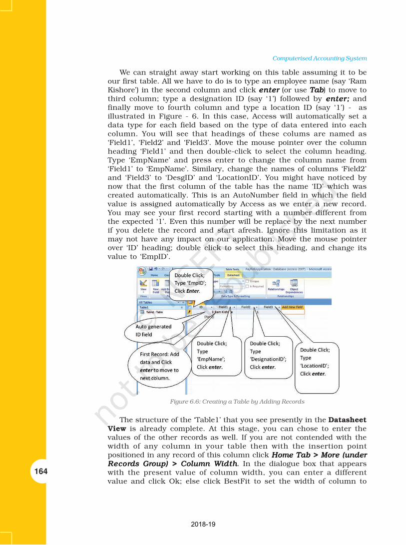
164
Computerised Accounting System
We can straight away start working on this table assuming it to beour first table. All we have to do is to type an employee name (say ‘RamKishore’) in the second column and click enterenterenterenterenter (or use TabTabTabTabTab) to move tothird column; type a designation ID (say ‘1’) followed by enter;enter;enter;enter;enter; andfinally move to fourth column and type a location ID (say ‘1’) - asillustrated in Figure - 6. In this case, Access will automatically set adata type for each field based on the type of data entered into eachcolumn. You will see that headings of these colums are named as‘Field1’, ‘Field2’ and ‘Field3’. Move the mouse pointer over the columnheading ‘Field1’ and then double-click to select the column heading.Type ‘EmpName’ and press enter to change the column name from‘Field1’ to ‘EmpName’. Similary, change the names of columns ‘Field2’and ‘Field3’ to ‘DesgID’ and ‘LocationID’. You might have noticed bynow that the first column of the table has the name ‘ID’ which wascreated automatically. This is an AutoNumber field in which the fieldvalue is assigned automatically by Access as we enter a new record.You may see your first record starting with a number different fromthe expected ‘1’. Even this number will be replace by the next numberif you delete the record and start afresh. Ignore this limitation as itmay not have any impact on our application. Move the mouse pointerover ‘ID’ heading; double click to select this heading, and change itsvalue to ‘EmpID’.
The structure of the ‘Table1’ that you see presently in the DatasheetView is already complete. At this stage, you can chose to enter thevalues of the other records as well. If you are not contended with thewidth of any column in your table then with the insertion pointpositioned in any record of this column click Home Tab > More (underHome Tab > More (underHome Tab > More (underHome Tab > More (underHome Tab > More (under
RecorRecorRecorRecorRecords Grds Grds Grds Grds Group) > Column Woup) > Column Woup) > Column Woup) > Column Woup) > Column Widthidthidthidthidth. In the dialogue box that appearswith the present value of column width, you can enter a differentvalue and click Ok; else click BestFit to set the width of column to
Figure 6.6: Creating a Table by Adding Records
2018-19

Database Management System for Accounting
165
accommodate the longest entry (See Figure 6.7). You can also do thisoperation in a simple manner using mouse while in Datasheet View.Position the pointer on the right column boundary of the selectedcolumn in the header row till the pointer changes to a vertical linewith a left-right-pointing arrow; then double click the left mouse-buttonto get the best fit.
Figure 6.7 : Column width adjustment
Did you notice that our first table is still named ‘Table1’ and it hasnot been saved yet. Click on the SaveSaveSaveSaveSave button on the Quick AccessQuick AccessQuick AccessQuick AccessQuick Access
toolbar on left hand top corner of window. A Save AsSave AsSave AsSave AsSave As dialogue box will
Figure 6.8 : Saving of the Table with intended Name
2018-19
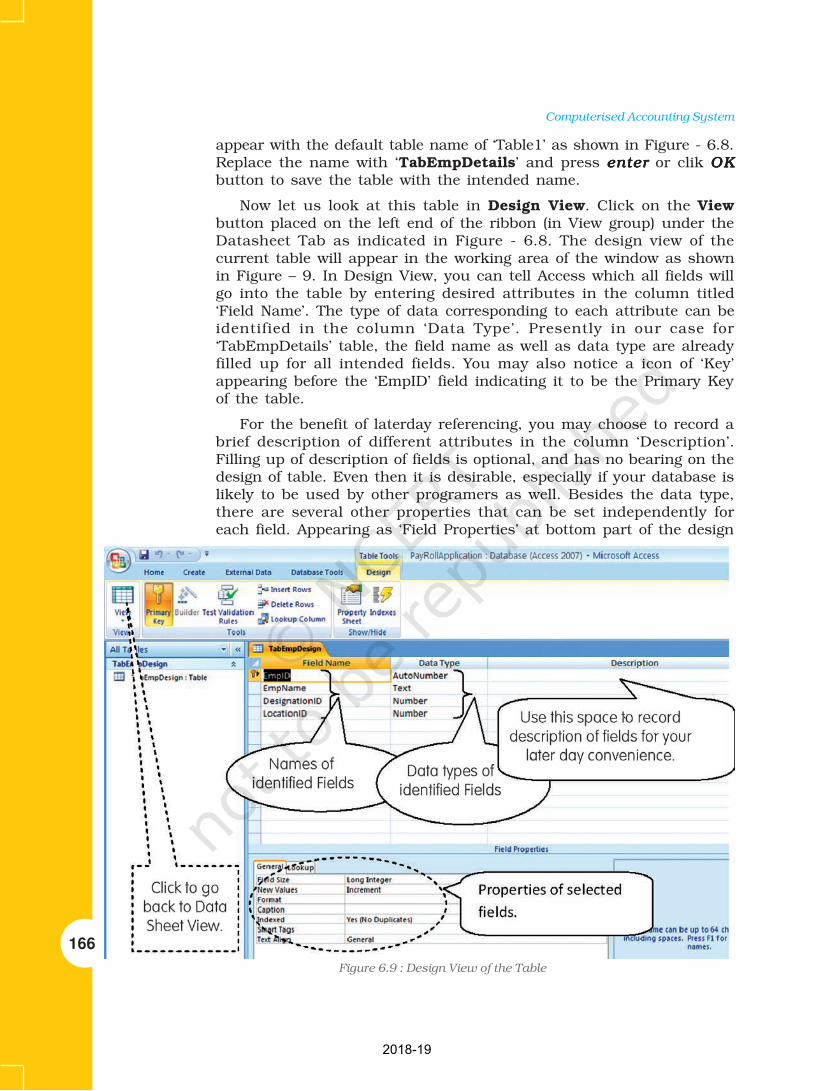
166
Computerised Accounting System
appear with the default table name of ‘Table1’ as shown in Figure - 6.8.Replace the name with ‘TabEmpDetails’ and press enterenterenterenterenter or clik OKOKOKOKOK
button to save the table with the intended name.
Now let us look at this table in Design View. Click on the Viewbutton placed on the left end of the ribbon (in View group) under theDatasheet Tab as indicated in Figure - 6.8. The design view of thecurrent table will appear in the working area of the window as shownin Figure – 9. In Design View, you can tell Access which all fields willgo into the table by entering desired attributes in the column titled‘Field Name’. The type of data corresponding to each attribute can beidentified in the column ‘Data Type’. Presently in our case for‘TabEmpDetails’ table, the field name as well as data type are alreadyfilled up for all intended fields. You may also notice a icon of ‘Key’appearing before the ‘EmpID’ field indicating it to be the Primary Keyof the table.
For the benefit of laterday referencing, you may choose to record abrief description of different attributes in the column ‘Description’.Filling up of description of fields is optional, and has no bearing on thedesign of table. Even then it is desirable, especially if your database islikely to be used by other programers as well. Besides the data type,there are several other properties that can be set independently foreach field. Appearing as ‘Field Properties’ at bottom part of the design
Figure 6.9 : Design View of the Table
2018-19

Database Management System for Accounting
167
view, these parameters of a field will vary with the choice of data type.A narration of each property (when you click the desired property) alsoappears in a hint box on right hand side, which makes understandingof field properties quiet simple. However, we will stick to defaultproperties of all fields, and ignore this area altogether.
Having fully completed the structure and data of our first table andalso having understood the various conccepts related to its design, wecan now move on and create rest of the four tables. Click on CreateTab > Table Button as illustrated in Figure – 10. The Data Sheet viewof the default table (Table1) will appear again. You can choose thisview or the Design View to create the rest of the tables and save themunder intended names. For your conveniene, the field names and datatypes of all five tables are summarised as under:
Sl. Field Name Data Type DescriptionNo.
1. TabEmpID
EmpID AutoNumber Unique employee ID – Primary Key.
EmpName Text
DesgID Number
LocationID Number
2. TabDesignations
DesgID AutoNumber Unique Designation ID – Primary Key.
Figure 6.10 : Creating New Table
2018-19

168
Computerised Accounting System
Designation Text
TA Number Transportation Allowance – fixed as perdesignation.
3. TabLocations
LocationID AutoNumber Unique Location ID – Primary Key.
Location Text
RateOfHRA Number % Rate of House Reent Allowance.
4. TabDARates
MonthID AutoNumber Unique MonthID – Primary Key.
SalMonth Text With values as ‘Jan-2007’, “Feb-2007” etc.
RateOfDA Number % Rate of Deanress Allowance.
5. TabMonthly Salary
SalaryID AutoNumer Unique SalaryID – Primary Key.
MonthID Number
EmpID Number
Basic Number Basic pay based on level & attendance ofemployee.
DedForPF Number Deduction for PF opted by employee & asper rules.
Having completed the designs of all data tables, we will now move onto the task of establishing relationships between different tables. Clickon the Databse ToolsDatabse ToolsDatabse ToolsDatabse ToolsDatabse Tools Tab and then RelationshipsRelationshipsRelationshipsRelationshipsRelationships button under Show/Show/Show/Show/Show/
Figure 6.11 : Creating Relationship between Table
2018-19

Database Management System for Accounting
169
HideHideHideHideHide group as shown in Figure - 6.11. In the working area, a ShowShowShowShowShow
TableTableTableTableTable dialogue box will appear as shown in Figure - 6.12. In case you
do not see this dialogue box click on Design > ShowDesign > ShowDesign > ShowDesign > ShowDesign > Show TableTableTableTableTable. In the
Show TableShow TableShow TableShow TableShow Table dialogue box, select a table and clik AddAddAddAddAdd button to add it
in the relationship window. Add all the five tables in this manner.
Close the Show Table dialogue box by clicking on CloseCloseCloseCloseClose button.
Figure 6.12 : Adding of Tables for Establishing relationships between them
In the working area you will see all five table objects, each detailing
the fields within them. You can reposition these table objects any
where within the relationship window. To do this, point the mouse
pointer in the caption area of the selected table object, hold down the
left mouse button and then drag the mouse to shift table to its new
location as shown in Figure -6.13. Now to create a relationship between
TabMonthlySalary and TabDARates, position the mouse pointer over
MonthID in the TabMonthlySalary table object, hold down the left mouse
button, drag the pointer right to MonthID in the TabDARates, and
then release the mouse button. A Edit RelationshipsEdit RelationshipsEdit RelationshipsEdit RelationshipsEdit Relationships dialogue box
will appear as soon as you release the mouse button. You will notice
that the dialogue box shows relationship type as One-To-Many
(see Figure-6.13).
2018-19

170
Computerised Accounting System
Access has determined the relationship type based on the fieldsselected for joining the two tables. Click on the CreateCreateCreateCreateCreate button. A blackline will appear joining the two tables at the common field. This line,also referred to as Join Line, establishes the relationship betweenTabMonthlySalary and TabDARates using the common field of MonthID.Remember, MonthID forms Primary Key in TabDARates and ForeignKey in TabMonthlySalary and hence is the relationship One-To-Manytype. You may now repeat above steps to establish other relationshipbetween the tables as indicated in Figure - 6.13. The overall relationshipbetween different tables are summarised as under:
Figure 6.13 : Relationship between different Tables
Table Related Table Common Field Relationship Type
TabDARates TabMonthlySalary MonthID One-To-Many
TabEmpDetails TabMonthlySalary EmpID One-To-Many
TabDesignations TabEmpDetails DesgnID One-To-Many
TabLocations TabEmpDetails LocationID One-To-Many
6.5 CREATION OF QUERY IN MICROSOFT ACCESS
As discussed in Section 4.0, we will now get on to the task of handlingcomputational fields of ‘DA’, ‘HRA’, ‘TA’, ‘GrossSalary’ and ‘NetSalary’using Queries. The Queries provide the real power to a database interms of its capabilities to answer more complex requests (orqueries). In case of Access, Queries provide the capability of combiningdata from multiple tables and placing specific conditions for the
2018-19

Database Management System for Accounting
171
retrieval of data. In its simplest form, you may consider a Query to beanother tabular view of your data showing information from one ormore tables.
Click on Create > Query Design. A Show TableShow TableShow TableShow TableShow Table dialogue box willappear with a Query Table in the background as shown in Figure – 6.14.In case you do not see this dialogue box click on Design > ShowDesign > ShowDesign > ShowDesign > ShowDesign > Show
TableTableTableTableTable. In the Show TableShow TableShow TableShow TableShow Table dialogue box, select a table and clik AddAddAddAddAdd
button to add it in the relationship window. Add all the five tables inthis manner. Close the Show Table dialogue box by clicking on CloseCloseCloseCloseClose
button. In working area above the Query Table, you will see all fivetable objects (with complete list of their fields) along with the one-to-one relationship that has been established between tables earlier. Youcan reposition these table objects in the manner discussed earlier. Inthe portion below Table objects, you will see blank columns thatrepresent columns in the Query results datasheet. These columns (seeFigure – 6.14) are also referred to as the Design GridDesign GridDesign GridDesign GridDesign Grid.
Figure 6.14 : Creation of Query
2018-19

172
Computerised Accounting System
In the first column of the design grid, click on the Table row. Adropdown button will appear on this cell. Click on the button to get thedropdown list of tables and click on ‘TabMonthlySal’. Now in the samecolumn, click on Field row and get the dropdown list of all fields in‘TabMonthlySal’. Click on the ‘SalaryID’ field. In this manner theSalaryID (from TabMonthlySal) has been selected for view in the Query.The above operation could have also been done simply by double clickingthe ‘SalaryID’ in the list box of TabMonthlySal object. You could havealso done this by positioning the mouse pointer on the identified fieldof a table object, held down the left mouse button, and dragged it tothe field row of the desired column of the design grid, and then releasedthe mouse button.
You shall take care to fill different fields from Table object into theDesign Grid in the same order in which you want to display thesefields in the Query Results data sheet. Now select any of the describedmethods to fill other columns of the design grid in the specified orderwith fields of Month ID (TabMonthlySalary), SalMonth (TabDARates),EmpName (TabEmpDetails), and Basic (TabMonthlySalary) asillustrated in Figure - 6.15. In case you may not require the need ofdisplaying MonthID, you may click on this field at the row marked as‘Show’ to uncheck the show-check-box. At this stage, if you click onthe RunRunRunRunRun button under ResultsResultsResultsResultsResults group of DesignDesignDesignDesignDesign Tab, you will see theresult of Query displayed with the fields of SalaryID, SalMonth,EmpName, and Basic. Clicking of ‘Run’ actually tells the Access to
Figure 6.15 : Creation of different Fields in the Query Table
2018-19

Database Management System for Accounting
173
execute all instructions stored by you in the Query, and to display theresults. You may adjust the column widths by any of the methodsdescribed earlier for Tables. Click on the SaveSaveSaveSaveSave button on the QuickAccess toolbar. At the Save As disalogue box, type QueryMonthlySalaryand click OKOKOKOKOK to save our Query.
Evidently our Query is not complete as we are not seeing thecomputational fields and the field of DedForPF in the DataSheet ViewDataSheet ViewDataSheet ViewDataSheet ViewDataSheet View.Go back to the Design Grid view by clicking on Design View underHome Tab. In the Design Grid, Click on the Field row of the first balnkcolumn (after Basic) and type ‘DA: [Basic]*[TabDARates.RateOfDA]/100’. In this expression, the word ‘DA’ coming before the colun(:) willbe treated as the name of the computational field which will appear asheading of the column. The rest of the typed part will form the actualexpression which will be evaluated and its value displayed on clickingof Run command. You may notice that in our expression for ‘DA’, wehave made use of ‘Basic’ field which is already forming a part of Queryby taking it within the square parenthesis ([ ]). We have also made useof ‘RateOFDA’ field which is not appearing in the Query columns; andfor this we recorded the corresponding Table name as well as Fieldname separated by a period (.) within the square parenthesis. It maybe easily comprehendable that the operator ‘*’ and ‘/’ stand formultiplication and division respectively. At this stage if you click onthe ‘Run’ command, you will notice the last field for ‘DA’ with itscomputed values for different employees as per the % DA Rates fordifferent months.
Come back to the design view (by Clicking Design ViewDesign ViewDesign ViewDesign ViewDesign View buttonunder ViewsViewsViewsViewsViews Group) and repeat above listed procedure to fill up thenext field of Query for computing HRA using the expression ‘HRA:[Basic]*[TabLocations.RateOfHRA]/100’. The next column in theQuery is for the TA field, which is to be included as such from theTable ‘TabDesignations’ using any of the methods enumerated earlier.Next, create the field for ‘Gross Salary’ by typing the expression‘GrossSalary: [Basic]+[DA]+[HRA]+[TA]’. Now we can also include thefield of ‘DedForPF’ from the ‘TabMonthlySalary’. Finally, we shallinclude the field of NetSalary using the simple expression ‘NetSalary:[GrossSalary]-[DedForPF]‘. At this stage, save your Query as instructedearlier and also run the ‘Run’ command to look back the outcome ofyour effort in the Data Sheet View.
While Figure -6.15 gives an illustration of the Design View of ourQuery, the Figure - 6.16 shows the Datasheet View of the Query. Yourview may be little different based on the actual data that you haveentered in different tables. As shown in Figure 6.16, you may noticethat the total dataset of the Query is composed of all data rowscorresponding to the Table ‘TabMonthlySalary’. You may restrict thedataset to any restricted values for any of the specified field. Forexample, we may want only the data corresponding to November 2007,
2018-19

174
Computerised Accounting System
for which the MonthID is ‘6’. With this objective, click on the Criteriarow under MonthID field and type ‘=6’ as shown in Figure - 6.17. Nowif you click on ‘Run’ command, you will see the data recordscorresponding only to the month (SalMonth) of Nov 2007’.
Figure 6.16 : Datasheet View of the Query
Figure 6.17 : Setting of Criteria and Sorting of Data in a Query
2018-19

Database Management System for Accounting
175
For a better presentation, you may also like to sort the records inascending or descending order against a chosen field of the Query.Thus, we may like to arrange the records of Nov.2007 as peralphabatically ordered names. For this, click on the Sort row belowthe EmpName field. Now Click on the pull down button that appearson the end of the cell and select AscendingAscendingAscendingAscendingAscending (see Figure – 6.17). Runthe Query and notice that the records are alphabatically arranged asper names of the employees.
6.6 CREATION OF FORMS IN MICROSOFT ACCESS
So far, we have learned the concepts behind organising the informationin a database using Tables and retrieving such information usingQueries. Now we will look into the mechanisms for placing informationinto the tables as and when the need arises. The Microsoft Accessprovides two primary mechanisms to achieve this goal. The first method,which we are already familiar with, is to simply bring up the table in awindow by double-clicking on it and adding information to the newblank row at the bottom. We can also make changes in any other rowas one would do in case of a spreadsheet. You can save the changes inthe table by clicking on the SaveSaveSaveSaveSave button on the Quick Access toolbar.
Box - 6.12Box - 6.12Box - 6.12Box - 6.12Box - 6.12
The Access 2007 provides facility for creation of a Simple Formwherein you can enter information for one record at a time. Access
also provides tools for creation of a Split Form which shows the
underlying datasheet in one half of the section and a Form in other
half for entering information in the record selected in the datasheet.
The two views in this form are synchronised so that scrolling in one
view causes the scrolling of other view to same location of the record.
As second mechanism for information handling (i.e. for addition,modification and deletion), the Access provides a user-friendly ForForForForFormsmsmsmsms
interface that allows users to enter information in a graphical form,and this information transparently passes to the underlyingdatabase. This method is more user-friendly for the data entry operator,though it may entail a little more work on the part of the databasedesigner.
For our Pays Roll Application, let us create a simple Form for theTable TabMonthlySalary – which is one table likely to be used morefrequently by the bill clerk. In the Navigation Pane ofPayRollApplication, Click once on the TabMonthlySalary. Havingselected the intended Table thus, Click on Create Create Create Create Create Tab and then onForForForForForm m m m m under Forms Group. The Form View of the TabMonthlySalarywill appear in the working area of Window showing first record of theTable as illustrated in Figure 18. At the bottom of the Form you willsee Navigation bar with buttons for ‘First Record’, ‘Previous Record’,
2018-19

176
Computerised Accounting System
‘Next Record’, ‘Last Record’ and ‘New Record’. In the middle of Navigationbar, you will also see the number of current record (e.g. 1 of 24). Clickon the buttons for Next Record a few times to scroll through a fewrecords in Form View. You may also click other buttons to understandtheir functions. If you click on New Record button, you will notice thata new record will get displayed with ‘SalaryID’SalaryID’SalaryID’SalaryID’SalaryID’ displaying (New) whileall other fields remaining blank. You may recall that SalaryID is thePrimary Key of this table with AutoNumber as its data type.
Figure 6.18 : Creation of Forms
We can make some changes in the size of data boxes and theirlocation within the Form. With this objective, let us first change theview of Form to Design View by clicking on Home > Design ViewHome > Design ViewHome > Design ViewHome > Design ViewHome > Design View. Inthe Design View, click on any of the Text Boxes. Move the mouse pointerto right end of the highlighted boundary of the Box till a Left-Rightarrow appears. Press the Left Mouse button, and holding it there movethe mouse towards left to reduce the width of Text Box to desired size.You will notice that the sizes of all Text Boxes have reducedautomatically. Now select all text boxes by clicking once on each boxwhile pressing the Shift key. Now move the Mouse pointer over any ofthe box till a sign with four arrows (similar to a + sign) appears. Pressthe Left Mouse button, and holding it there move the mouse towardsright to shift the Text Boxes to a more central location.
2018-19

Database Management System for Accounting
177
We know that in TabMonthlySalary, the field of MonthID is a ForeignKey. In order to have meaningful values in our final Query (i.e.QueryMonthlySalary), this field shall contain only those values thatare already stored in TabDARates. We can impose this condition in theForm while we are in Design View. Click and select the MonthID TextBox. Keeping the mouse pointer within this Box, click the right mousebutton and select Change To > Combo Box Change To > Combo Box Change To > Combo Box Change To > Combo Box Change To > Combo Box as illustrated in Figure –19.You will notice that the Text Box of MonthID field will change to aCombo Box with a pull down button appended at the end of box. Withthe MonthIDMonthIDMonthIDMonthIDMonthID ComboBox still selected, click on the Property SheetProperty SheetProperty SheetProperty SheetProperty Sheet
Button under Tools Group. This will open up the Property Sheet of theMonthID Combo Box as shown in Figure - 6.20. In the DataDataDataDataData Tab ofProperty Sheet (which may be already open before you), click on thecombocombocombocombocombo button against ‘Row SourceRow SourceRow SourceRow SourceRow Source’ property to see the pull down listof Tables; and select ‘TabDARates’. Note that you will be able to seethe Combo option under ‘Row Source’ property, only if, the ‘Row SourceType’ property is selected as ‘Table/Query’. Ensure that the ‘BoundColumn’ property has a value of ‘1’, which corresponds to the FirstColumn – i.e. ‘MonthID’ – of the ‘TabDARates’. Having thus reset theproperty of MonthID field of the form, change the view to Form View.You will notice that the Form now shows a Combo Box against theMonthID field and in its pull down list only those MonthIDs will appearwhich are already stored in the TabDARates. You may realise that inTabMonthlySalary, the field of EmpID also needs to be given similartreatment; and its values shall be restricted to the values of ‘EmpID’given in the TabEmpDetails.
Figure 6.19 : Changing of Textbox to a Combo Box in the Form Design View
2018-19

178
Computerised Accounting System
Many more changes can possibly be done in our Form to make itmore user-friendly. However, these may entail the use of ‘Macro Builder’,‘Query/Expression Builder’ and ‘Code Builder’. These topics are beyondthe scope this book, though you may explore them gradually afterdeveloping familiarity with presently covered areas of Accessprogramming. You may also develop suitable designs of Forms for otherTables of the Payroll application.
6.7 CREATION OF REPORTS IN MICROSOFTACCESS
Information stored in a Table or Query can be easily printed while it isin Datasheet view. This can be done by using PrintPrintPrintPrintPrint command givenunder Office Button on left hand top corner of the window. Even aForm view can be directly printed in similar manner. A Report is alsoused for the print purpose, though it allows for more flexibility inselecting the fields to print, and to have more control on the overalllayout and format of the print output. The Report in Access is thusanother object which is designed to print information from the databaseon to the screen, or to a file or directly to the printer.
Here also you can take the elaborate route of step-by-step design aswas done in case of Tables, Query or Form. However in this case, youmay find the Report WReport WReport WReport WReport Wizarizarizarizarizard d d d d becoming a more favorable tool as itguides the designer through a series of dialogue boxes to create themost suitable Report.
Figure 6.20 : Setting the Properties of Combo Box
2018-19

Database Management System for Accounting
179
Evidently in our case, we will be interested in generating the Report
for the ‘QueryMonthlySalary’. With this intent, Click on
‘QueryMonthlySalary’ in the Navigation Pane, then click on CreateCreateCreateCreateCreate
Tab, and then on Report WReport WReport WReport WReport Wizarizarizarizarizard d d d d under Reports Group. In the dialogue
box that appears with QueryMonthlySalary Query already selected,
move all fields from the Available FieldsAvailable FieldsAvailable FieldsAvailable FieldsAvailable Fields List Box to the Selected Fields
List Box using appropriate ArrowArrowArrowArrowArrow button as shown in Figure - 6.21.
Click NextNextNextNextNext to see the second dialogue box asking for Grouping Levels.
Here select ‘SalMonth’ and click on the Arrow button (else double click
the ‘SalMonth’) to print data in groups of different salary months (See
Figure – 6.21). Click NextNextNextNextNext to reach the third dialogue box asking for
sorting order of the records. Here you can click on the Pull-down Arrow
next to the first text box and then select ‘SalaryID’ from the drop down
list so as to arrange the records in ascending order of the salary ID
within each data group - as illustrated in Figure - 6.22. Click Next to
see the dialogue box for layout of the Report. Retain the default ‘Stepped’
layout but change the orientation of Report to ‘Landscape’ so as to see
all the columns of the Report in a single page view (see Figure - 6.22).
Again Click NextNextNextNextNext to see the dialogue box for selecting style of Report.
You may choose any style and later on experiment with the others as
well. One more click of NextNextNextNextNext will take you to the dialogue box seeking
the name of Report object. Type ReportMonthlySalary and click on
the FinishFinishFinishFinishFinish button to see the Report appearing in working area of window
in its Print Preview form.
Figure 6.21 : Report Wizard Dialogue Boxes
2018-19

180
Computerised Accounting System
You may notice that the extent of data in above designed Report islimited as per the Criteria laid down in our Query‘QueryMonthlySalary’. By changing the Query suitably, we can modifythe Report for generating monthly as well as annual Pay Rolls. We canalso change the Criteria of our Query to get individual Report for eachmonth (i.e. Pay Slip) or for the whole of year (i.e. Annual Statement).
Figure 6.22 : Report Wizard Dialogue Boxes
Figure 6.23 : Adding of Sum Expression in the Report
2018-19

Database Management System for Accounting
181
We may like to improve the Report further by getting sum total ofall the values under different columns for each group. For example,we may want to see the total Basic of all employees for November 2007group. For such modification, open the Report in Design View by Clickingon HomeHomeHomeHomeHome Tab and then clicking on Design ViewDesign ViewDesign ViewDesign ViewDesign View under Views Group.In the design view as shown in Figure - 6.23, select the field Basic byclicking it once. Now click on TotalsTotalsTotalsTotalsTotals under ‘Grouping and Totals’Group of DesignDesignDesignDesignDesign Tab. In the pull down menu that appears, click on‘Sum’. You will notice that an expression ‘=Sum([Basic])’ will appearbelow the Basic Text Box. You can repeat above steps with other fieldscontaining numerical (both stored as well as computed) values. Now ifyou click on View button (i.e. click Design > Report ViewDesign > Report ViewDesign > Report ViewDesign > Report ViewDesign > Report View), you willsee the sum total of each column (with in each group) appearing in thereport as illustrated in Figure 6.24.
Figure 6.24 : Print Preview of Monthly Salary Report
At this stage, close the Report by clicking on the Cross buttonimmediately above the report. Save the application once again byclicking on the SaveSaveSaveSaveSave button under Quick Access Bar. Our PayRollApplication in Access has been completed and saved. You may nowclose your application by clicking on the CloseCloseCloseCloseClose button under ‘OfficeOfficeOfficeOfficeOffice
ButtonButtonButtonButtonButton’ or by simply clicking on the Cross button at right-hand topcorner of the window.
2018-19

182
Computerised Accounting System
SummarySummarySummarySummarySummary
• Database Management System (DBMS) provides a variety of software toolsfor organising, processing and querying data in a flexible manner.MS-Access, Oracle, SQL Server, IBM-DB2 are examples of DBMS software.
• In DBMS, data is organised in tables (similar to a file). A table has anumber of rows (or records) and columns (or fields or attributes). Eachrow contains a record of information, for example of an account head or aparty or a transaction as per the need. The information in a row consistsof a sequence of columns or attributes, such as transaction number,transaction date, etc, or it could be party’s name, party’s address, etc.
• One of the tasks in analysis of requirement is to identify and list out theinformation required including its elements. These elements of informationbecome columns (attributes) in appropriate tables.
• Data (set of attributes) should be logically structured so as to put them invarious tables. The goal of such structuring is to reduce data redundancy,to achieve data consistency as well as to enhance efficiency for adding,updating and querying operations on database.
• Normalisation is the process for removing data redundancy.
• Since the data stored in different tables may be related, such relationshipis implemented by establishing links between tables. The database createdon the basis of such relationships between different tables is calledrelational database.
• Relationship between tables is established with the help of primary keyand foreign key. Primary key consists of minimum possible one or morethan one attributes of a table, which uniquely identifies each row of thattable. Foreign key consists of set of attributes, which from primary key inanother (related) table.
• Most of Computerised Accounting Systems are multi-user systems. Thesesystems use ‘server database’ unlike single-user (or desktop) systems using‘desktop database’. In a multi user system, a user interacts with thesoftware though the user interface, which is also termed as ‘front-end’.Database, which is kept on a server, is termed as a ‘back-end’.
• MS-Access is an example of ‘desktop database’. Oracle, SQL Server, IBM-DB2 is examples of ‘server databases’, Desktop databases may be satisfactoryfor SOHO (Small Office Home Office) organisations as they offer inexpensiveand simple solutions to many of business data storage and processingrequirements.
• In order to provide security and consistency of data, database is not directlyaccessible to users. Any addition or retrieval of information from databaseis done by user-friendly programs. Database is thus rightly referred to as‘back-end’ while the interactive program, that includes user interface, istermed as ‘front-end’ of a database application.
2018-19

Database Management System for Accounting
183
EXERCISE
Q1. MULTIPLE CHOICE QUESTIONS
1. ‘DBMS’ stands for:
a. Drawing Board Management Software
b. Dividend Based Marking System
c. Data Base Management System
d. Data Base Marking Software.
2. MS Access is a:
a. Word processing Software
b. Presentation Software
c. Spread sheet Software
d. Data Base Management Software.
3. The term ‘field’ as applied to database table means:
a. Vertical column of the table
b. Size of the table
c. Horizontal row of the table
d. Name of the table.
4. The term ‘record’ as applied to a database table mean:
a. Vertical column of the table
b. Size of the table
c. Horizontal row of the table
d. Name of the table.
5. The common fields used in a relationship between tables are called:
a. Joint fields
b. Main fields
c. Key fields
d. Table fields.
6. The existence of data in a Primary key field is:
a. Not necessarily required
b. Required but need not be unique
c. Required and must be unique
d. All of above
2018-19

184
Computerised Accounting System
7. The existence of data in a secondary key field is :
a. Not necessarily required
b. Required but need not be unique
c. Required and must be unique
d. All of above
8. SQL stands for:
a. Simple Questions Language
b. Simple Que line up
c. Singular Quantity Loading
d. Structured Que Language
9. The default extension of MS Access (2007) file is :
a. .accbd
b. .exl
c. .doc
d. .exe
10. Wizards in MS Access means
a. Person who developing progamme
b. Tools for simplifying the programme usage
c. Relating between tables
d. Reporting generated by programme.
11. ‘Join line’ in the context of Access Tables means:
a. Graphical representation of relationship between tables
b. Lines bonding the data within table
c. Line connecting two fields of a table
d. Line connecting two record of a table.
12. In order to retrieve select data meeting a specified criteria from two different
tables of Access database, we may make use of :
a. Table
b. Query
c. Form
d. Report.
2018-19

Database Management System for Accounting
185
13. To expect a well formatted printable data from Access database, we may use:
a. Table
b. Query
c. Form
d. Report.
Q2. ANSWER THE FOLLOWING QUESTIONS
1. What do you understand by DBMS. Give names of two commarly availableDBMS softwares?
2. Differentiate between ‘Desktop database’ and ‘Server database’. List thecriteria that may help you in selecting appropriate database?
3. With suitable example illustrate the meaning of ‘attributes’ as applied todatabase?
4. Why do we seek to split up in formation into different tables rather thanconfine it to a single table?
5. What do you understand by terms ‘key field’ , ‘primary key’ and ‘secondarykey’ in a database?
6. List the conventions that you will follow, while naming different fields of a table?
7. What are the uses of ‘query’ object in Access program?
8. What do you understand by ‘Form’ object in Access and how are they useful?
9. What is the purpose of ‘report’ object in Access program?
10. What do you understand by database? What are the ways in which data isstored and queried in an Access database?
11. What are the advantages of Access over Excel?
12. Describe in brief the function of ‘Table’, ‘Query’, ‘Form’ and ‘Report’ object ofAccess program?
Q3. SKILL REVIEW
1. You are starting to plan ahead for you job search. You decide to maintain adatabase of company information in Access.
2. Search for at least eight companies. You wish to apply for include companyname, address, telephone and fax numbers. If possible, also include the nameof contact person in their human resorce department.
3. Create job search company safer, accounting database.
4. Open the company information table.
5. Enter at least records for the companies you researched.
6. Adjust column widths, as necessary.
7. Sort the records in ascending order of Name of Company.
8. Preview Table
2018-19

186
Computerised Accounting System
9. Format all record to a smaller font size.
10. Change the page layout so that entire table fit on the page.
11. Close company information table.
12. Close Job Search Company, acedb database.
ANSWER
Q.1.1. c. 2. d. 3. a. 4. c 5. c 6. c. 7. a
8. d. 9. a. 10. b. 11. a. 12. b. 13. d.
2018-19