20171207 writeup pollution...

Exporting Pollution

Itzhak Ben-David Fisher College of Business, The Ohio State University, and NBER

Stefanie Kleimeier

Maastricht University, School of Business and Economics, Open Universiteit, Faculty of Management, Science & Technology, and University of Stellenbosch Business School

Michael Viehs

University of Oxford, Smith School of Enterprise and the Environment, and Hermes Investment Management, Hermes EOS

December 2017

Abstract

Despite the awareness of the detrimental impact of CO2 pollution on world climate, countries vary widely in how they design and enforce environmental laws. Using novel micro data about firms’ CO2 emission levels in their home and foreign countries we document that firms headquartered in countries with strict environmental policies perform their polluting activities abroad, in countries with weak policies, relative to the policies in their home countries. Our study helps shedding light on the effectiveness of countries’ environmental laws and enforcement, as well as how firms respond to these policies.

Keywords: Pollution, Production, Pollution Haven HypothesisJEL Classification: N50, O13, P18, Q56, R11

_____________________

* We are grateful to CDP (Carbon Disclosure Project), for sharing the climate change data with us. All views expressed in this paper are those of the authors and not necessarily those of Hermes Investment Management or Hermes EOS.

2

1 Introduction

Countries apply different degrees of stringency towards combatting CO2 pollution,

despite the wide agreement among climate scientists that such pollution is the primary cause of

global warming. Around the globe, countries take different approaches, ranging from stringent

environmental laws and strict enforcement to lax rules and turning a blind eye to polluting

activities. Some economists have proposed the Pollution Haven Hypothesis (PHH), that polluting

activities by firms are performed in countries with weak environmental policies (Eskeland and

Harrison 2003, Cole 2004, among many others). One implication of the PHH is that strict

environmental policies by individual countries might have little effect on global pollution levels,

since they crowd out pollution toward countries with more lenient environmental policies.

Previous studies (discussed below) attempts to test the PHH used aggregate data (e.g., country

level) and never could measure pollution directly.

In this study, we test the PHH using a unique panel dataset of CO2 emissions by large

public firms in each country of operation. Using these data, coupled with country-year-level

information on the stringency of national environmental policies, both in the firms’ home

markets and abroad, we test whether firms actually pollute more in countries with weak

environmental laws and enforcement. Our results provide novel direct evidence for the PHH in

addition to new results from the cross-section of firms.

The main prediction of the PHH is that polluting industrial activities take place more

intensely in countries with weaker environmental policies. This occurs due to a combination of

both demand and supply effects. Firms demand to transfer their polluting operations to countries

with weak environmental laws and weak enforcement. The idea is that restricting emissions is

costly for firms; therefore, they seek emission-friendly environmental policies. In turn, countries

3

may be able to attract polluting firms by providing weak environmental policies and lax

enforcement of those policies. Countries impose relaxed environmental policies so they can

benefit from the economic activity (e.g., employment, investments) that industrial production

brings. While identifying demand effects from supply effects is important, previous literature

struggled even with providing direct evidence for the PHH; our study focuses on providing direct

micro-evidence for the equilibrium outcome rather than identifying the demand and supply

effects.

We provide two main sets of tests for the PHH. The first set of tests is based on aggregate

firm-year data in which we examine whether firms tend to pollute more abroad given the

strictness of environmental policies in their home country. Our results show that indeed, firms

headquartered in countries that have stricter environmental policies are inclined to perform more

of their polluting activities abroad. Our results are robust to a variety of controls at the industry

and country levels.

In the second set of tests, we draw on the literature in international trade and use a gravity

model. The idea behind these tests is that strict environmental policies in the home country may

push polluting activities abroad, while lax environmental policies in the target country may

attract such activities. Indeed, we document that the “distance”, i.e., the difference between the

strictness in the home country and destination country, is a strong predictor of pollution in the

destination country.

Overall, we find support for the PHH. Our results show that indeed firms perform their

polluting activities outside borders of their home country when their country imposes strict

environmental policies. Or, in other words, strict environmental regulation implies lower firm-

4

level emissions at home. Furthermore, countries with lax environmental policies tend to attract

polluting activities from countries with stricter policies.

Our work follows decades of research in which the PHH was developed by

environmental economists. Leonard and Duerksen (1980) and Walter (1982) conducted early

studies proposing a link between aggregate industrial pollution and countries’ environmental

laws. Later, several studies explored the theoretical conditions under which the PHH is likely to

be confirmed in the data. Socolow (2006) analyzes the different paths that policy can take in

order to reduce carbon emission over the next 50 years. Numerous studies correlate aggregate

measures of trade and investment with environmental policy. Taylor (2005) explores the

theoretical implications of PHH and reviews the literature on the topic. Bommer (1999) proposes

a theoretical extension to the PHH, showing that producers relocate their manufacturing facilities

to countries with low environmental law enforcement to warn home regulators against further

tightening environmental regulations.

Prior studies generally test the PHH mostly with aggregate data and indirect and crude

proxies for pollution. Several studies correlate aggregate industrial activity and the stringency of

environmental laws in home countries compared to the target countries (Shafik and

Bandyopadhyay 1992, List 2001, Cole and Elliott 2005, MacDermott 2009, Wagner and

Timmins 2009, Kalamova and Johnstone 2011, Ben Kheder and Zugravu 2012). Many of these

studies are not able to observe environmental regulation, and thus use actual pollution, pollution

abatement costs, or country income levels as proxies for the weakness of regulation. Other

studies find a correlation between trade flows and country-level or industry-level environmental

regulations (Cole 2004, Levinson and Taylor 2008, Kellenberg 2009, Kearsley and Riddel 2010).

Grossman and Krueger (1995) document that income per capita is negatively correlated with

5

pollution levels. Milimet and List (2004); Aliyu (2005); and Mulatu, Gerlagh, Rigby, and

Wossink (2010) find that the location of manufacturing facilities in developed countries (e.g.,

OECD, European countries) is correlated with the stringency of the home environmental policy.

Peters, Marland, Le Quéré, Boden, Canadell, and Raupach (2012) show that global carbon

emissions declined temporarily around the 2008 financial crisis due to a decline in global

production. Kellenberg (2009) uses multinational industry-level data and finds that

environmental policies prevent polluting industrial activities. Esty and Porter (2005) argue that

countries’ environmental policies not only depend on income levels but also on the social and

cultural context.

At the micro level, there is limited and, again, only indirect evidence on firm pollution

and environmental policies. To our best knowledge, all studies that use micro-level data estimate

whether firms are more likely to have facilities in countries with weak environmental policies

without observing the actual pollution levels. Sen (2015) estimates a structural model that

proposes that stringent environmental laws and enforcement lead to greater innovation and

research and development (R&D) activity. He finds confirming evidence for the model in the

auto industry. Dam and Scholtens (2012) document that firms with a lower environmental

responsibility qualitative index score are more likely to manufacture in countries with weak

environmental regulation. This index is composed by the Ethical Investment Research Service

and characterizes firms according to their ethical conduct on multiple dimensions. Becker and

Henderson (2000, 2001) find that industries in the United States reacted to a specific

environmental regulation that applied only to large plants by transitioning production to smaller

facilities. Ben Kheder and Zugravu (2012) use firm-level location data to study location

decisions with respect to local environmental laws. They find that firms are more likely to have

6

facilities in countries with weaker environmental regulations, as measured by the degree of

international environmental agreements, NGO (non-governmental organizations) activity, and

energy efficiency.

2 Data Description

2.1 CO2 Emission Data

We use several sources of data. Our main data source is a large database that contains

self-reported responses of firms about CO2 emissions at the global and national level provided by

CDP. CDP is a United Kingdom-based “not-for-profit charity that runs the global disclosure

system for investors, firms, cities, states and regions to manage their environmental impacts”

(CDP 2017). As of 2017, more than 800 institutional investors with US$100 trillion in assets

were supporting the CDP and its initiatives. Since its inception, CDP has experienced a

tremendous growth in the number of institutional investors signing up for CDP and also in the

assets under management represented by those institutional investors. Also, it has grown

immensely from just surveying UK-based FTSE firms to obtaining climate change and pollution

information from firms all around the world.

Our dataset consists of the annual survey questionnaires and the corresponding answers

given by firms between 2008 and 2016. Over this period, CDP increased its outreach from about

3,000 to nearly 6,000 firms worldwide. CDP sends its survey to the largest firms worldwide,

most of which have publically traded equity. The questionnaires ask firms about their CO2

emissions, the firms’ various approaches to combatting climate change, and the practices they

use to manage the potential risks stemming from climate change. In this study, we focus in

7

particular on those questions in the questionnaires which ask firms about their levels of CO2

emissions, both directly and indirectly emitted from their operations. The answers to these

questions allow us to directly measure firm level emissions and identify the country in which

these emissions are made. Overall, the firms in our sample emit CO2 in more than 200 different

countries. We have pollution information on firms that operate in multiple countries as well as

firms that operate in a single country (about 11% of the sample). As mentioned before, this is a

clear data advantage over other studies that use micro-data; prior studies focus on multinational

firms exclusively and thus ignore the decision to transfer some operations outside the home

country (see, for example, Dam and Scholtens 2012). We create a panel dataset containing

annual CO2 emission information for firms in each country in which they operate.

There are two measures of emissions: Scope 1 and Scope 2. Scope 1 emissions are the

total CO2 emissions that stem directly from the operations of the reporting firms, in metric tons.

Scope 2 emissions are the total CO2 emissions arising from the electricity that the firm purchases

to run its operations and over which it does not have direct influence. This quantity is estimated

by the firm based on the breakdown of the electricity sources used in the respective country.

Hence, Scope 2 measures emissions that took place upstream in the supply chain, in metric tons.

One caveat to this dataset is that it contains information voluntarily self-reported by

firms. The motivation for firms to report their degree of pollution is pressure from institutional

investors and regulators for greater transparency regarding the environmental impacts of their

business and how climate change affects the long-run viability of their business. Investors,

especially long-term institutional investors such as pension funds and insurance companies, put

this pressure on firms because they need to understand the long-run implications of tightening

climate change and environmental regulation resulting from the Paris Agreement on climate

8

change which had been agreed on in 2015 and subsequently implemented by most signatory

countries. Having said that, institutional investors are interested in learning about firms’

exposure towards climate change and environmental issues to identify business models which are

at risk or less resilient.

Despite the self-reported nature of our data, there are good reasons to believe that the

information on emissions are accurate and close to actual emissions. First, many firms report

exactly the same statistics in sustainability reports, which are published alongside their annual

reports. Second, some firms have started to have their auditors approve the statistics in the

sustainability reports. If the self-reporting contains any sort of selection bias, it should bias our

results against finding supporting evidence for the PHH (firms might attempt to hide reporting

emission activity in foreign countries). If anything, our results are likely to show a lower bound

for the effect, since pollution reporting is voluntary and the firms that report may be less

aggressive then non-reporters.

Given that the CDP is an investor-supported initiative, there is also a natural regulatory

mechanism at work which ensures that the reported information by firms is generally credible

and trustworthy. Through engagement with firms, investors are pushing companies to participate

in the CDP and report through it, but also facilitates a discussion between CDP and firms in

cases where there is disagreement regarding the scores that CDP assigns to the firms’ responses

to the survey. After all, firms have an incentive to report truthful information through CDP:

Reporting inaccurate information on its climate change policies and emission levels could carry

significant litigation risks in some jurisdictions.

We can also provide some comfort for the quality of the data and hence the results. When

we restrict the sample to those observations where the emissions information has been externally

9

verified, the main results have similar results with the main sample results. We discuss these

robustness tests and results together with discussion of the main tests in Section 3.

2.2 Environmental Laws and Enforcement Data

The other major component for our analysis is data about the strictness of environmental

laws and enforcement at the country level. We use a dataset compiled by the World Economic

Forum (WEF) that covers the 2008–2015 period and which is available on an annual basis for

150 countries. Countries are assigned two rankings from one to seven: (1) the stringency of their

environmental regulation (SER) and (2) how strictly these laws are enforced (EER).

We assume that a country needs both components, laws and enforcement, to have a

potent environmental policy in place. Stated differently, there is an inherent interaction between

these two dimensions: Strict environmental laws that make a difference also need to be enforced.

The scores for environmental strictness and environmental enforcement have correlation

of 0.97, which induces multicollinearity when both are introduced to regression analysis

simultaneously. To remedy this issue, we adopt three approaches. The first is to combine the two

scores into a single variable: 𝑆𝐸𝐸𝑅 = %&𝑆𝐸𝑅 ∗ 𝐸𝐸𝑅. We call this measure Stringency and

Enforcement of Environmental Regulation, or SEER, and its values range from 0 to 7. The other

two approaches involve (1) examining the effect of each variable in isolation, and (2)

orthogonalizing the variables and introduce both into the regressions.

10

2.3 Firm-Level Financial Data

We also use commonly used databases to obtain financial information about

multinational firms and the countries in which they operate. We use firm-specific financial

statement data from Worldscope and country-specific macro-economic data from the World

Bank’s World Development Indicators. We also collect the classical gravity proxies such as

geographical distance, common border, colonial history, and trade between the firm’s home

country and the country in which it emits CO2. These proxies come from the Distancefromto.net,

Andrew Rose’s website (see Glick and Rose 2016) and the IMF’s Direction of Trade Statistics.

Finally, as our measure of corporate governance quality of firms, we use the corporate

governance score, CGVSCORE, from Asset4 which is nowadays widely used in research but also

by long-term institutional investors. The score ranges between 0 and 100 and measures in

percent the quality of a company’s governance systems and processes, ranging from board

structure, over compensation arrangements to firm’s treatment of shareholder rights. A higher

CGVSCORE value indicates better governance. Variable definitions and sources as well as

descriptive statistics can be found in Appendix Table 1.

The final dataset is a three-dimensional panel of the firm-country-year, which contains

the amount of CO2 emissions by each firm in each country in each year. Naturally, most of our

emission observations have the value of zero, as each firm have operations only in a few

countries.

11

2.4 Summary Statistics

2.4.1 Pollution and Environmental Regulation Over Time

Table 1 reports some summary statistics over the sample period. It provides the number

of unique firms, their global and home-country emissions, and the number of countries in which

each firm has emissions, everything reported across the period from 2008 to 2015. For the

average firm, global emissions in tons decrease over time for Scope 1 and 2. Noteworthy,

however, is the fact that, on average, the majority of emissions arise from the direct, Scope 1

emissions. On average Scope 1 emissions decrease from about 5 million metric tons to 2.6

million. Most CO2 is emitted at home, but the share of home emissions in global emissions

decreases substantially over time (from 72% to about 57% for Scope 1 emissions). Thus, over

time, the average firm emits more abroad. In addition, the number of countries where the average

firm’s emissions take place increases from 6.0 (6.8) countries in 2008 to 9.0 (10.6) in 2015 for

Scope 1 (Scope 2). Taken together, these results could be a first indication that firms shift

emissions abroad over time. However, the observed trends might simply be driven by an

increasing globalization of firms and unrelated to environmental regulation. Therefore, in the

empirical results that follow in this paper, we control for the increasing globalization in various

ways.

As described earlier, our measure of environmental regulation is SEER, which is the

product of measures of the environmental strictness score (ranging from 0 to 7) and the

environmental enforcement score (ranging from 0 to 7). Panel C of Table 1 indicates that SEER

generally increases over time, both on average and at the median. However, we also observe a

convergence of SEER across the different countries, as indicated in the last three columns of

Panel C in Table 1. The results indicate that environmental regulation is fairly stable at the global

12

average. However, on a country level, there are distinct developments. Among the 50 countries

with the strongest regulation in 2008, standards are slightly weakening over time. Among the 50

countries with the weakest regulation in 2008, standards are generally strengthening. This

finding suggests a convergence of environmental regulation over time. Furthermore, comparing

means and medians reveals that the distribution of environmental regulation is skewed, with

most countries being weakly regulated.

Environmental regulation varies a lot across the globe. Figure 1 presents country-level

environmental regulation at the beginning and end of our sample period using heat maps. The

map shows a general improvement in environmental regulation over time; however, there are

large regions where environmental regulation is weak, especially in developing countries in

Africa, South America, and Asia.

Figure 2 visualizes the relationship between environmental regulation in the firm’s home

country (as measured by our proxy SEER) and firm-level emissions abroad. Each bubble

represents all pooled firm-year observations and the respective SEER category for environmental

regulation in the home country, with 7 representing the most stringent regulation and 1 the

laxest. Panel A shows Scope 1 emissions, and Panel B shows Scope 2 emissions. Two

observations can be made: First, bubbles move from the top left to the bottom right, implying

that firms in home countries with stronger environmental regulation pollute less at home and thus

shift a higher fraction of their total emissions to foreign countries. Second, bubbles get bigger as

we move from the top left to the bottom right, indicating that per dollar of firm assets, firms in

countries with stronger regulations emit more tons of CO2 abroad. This pattern is similar for

Scope 1 and 2 emissions and supports the PHH with respect to home-country environmental

regulation.

13

2.4.2 Firm-level summary statistics

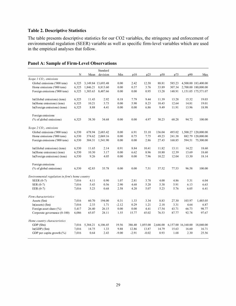
Table 2 presents summary statistics for our sample firms. We find that on average, firms

emit more in their home countries than abroad (1.85 million tons vs. 1.3 million tons for Scope 1

emissions and 0.37 million tons vs. 0.3 million tons for Scope 2 emission). On average, 38.3%

(42.8%) of firms’ Scope 1 (Scope 2) emissions are emitted abroad. Regarding the firms’

exposures to environmental regulation, we find that the average SEER for a firm in our sample is

4.11, while the strictness score of the environmental regulation is on average 5.4 and the score

for the enforcement of environmental regulation is only 5.23. The average firm in our sample has

US$ 60.7 million assets and a foreign asset share of 26.4%. Our corporate governance variable

indicates that the average firm in our sample has a governance score of 65 (out of a score

between 0 and 100). We provide further country-level statistics in Table 2 which we will also use

in our empirical analyses as control variables.

3 Empirical Design and Results

3.1 Polluting at Home or Foreign Country

To test whether firms pollute more in countries with weak environmental policies, that is,

low levels of SEER, we explore the determinants of location of pollution using the following

dependent variables: logged global emissions of CO2, logged emissions in home country, logged

emissions in foreign countries, and foreign emissions in percentage of global emissions. Our

main variable of interest is SEER, the combined variable of environmental strictness and

enforcement strictness. Other independent variables include logged firm assets, share of foreign

14

assets, logged gross domestic product (GDP) in home country, in addition to year and industry

fixed effects. Standard errors are clustered by firm.

The results are presented in Table 3, where Panel A shows evidence for Scope 1

emissions and Panel B shows evidence for Scope 2 emissions. Columns (1) and (2) regress the

logged global emissions in tons on SEER and control variables. The coefficient on SEER is

negative, indicating that firms with strict environmental policy in their home country pollute less.

An increase in one standard deviation in SEER (0.90) is associated with about global emissions

that are lower by 20% (controlling for firm size, home country characteristics, year and industry

fixed effects). We find results in similar magnitude in Panel B, about Scope 2 emissions. In the

regressions presented in column (2) of Panels A and B of Table 3, we also control for a firm’s

share of assets which are located abroad. We include this independent variable to control for the

higher likelihood of foreign emissions when the firm has more assets located abroad. Our

previously documented results remain unchanged and we find that a firm’s share of foreign

assets does not influence its global emission levels in either way.

In columns (3)-(4), and (5)-(6) we explore the emissions in logged tons of CO2 at the

home country and in foreign countries, respectively. Because some firms have zero emissions at

their home countries, we use Tobit for this specification.1 Here the effect is larger: an increase in

one standard deviation of SEER is associated with emissions at home that are lower by up to

37%. In contrast, an increase by one standard deviation in the strictness of the environmental

policies at home is associated with emissions greater by up to 30% in foreign countries. As for

Scope 2 emissions, Panel B shows that a one standard deviation increase in SEER is correlated

with a decrease in local emissions of 23% and an increase in foreign emissions of 32%. For both, 1 As the fraction of observations that is censored is relatively low in our sample, we re-estimate all Tobit regressions in Tables 3 to 5 and Appendix Tables 3 and 4 as OLS. Our results are robust and available upon request.

15

Scope 1 and Scope 2 emissions at home, we find that a higher foreign asset share significantly

reduces a firm’s emissions at home, however, this effect is not dominating the influence from

country-wide environmental legislation and the enforcement thereof.

Columns (7) to (8) reaffirm the previous findings by documenting the relation between

the percentage of foreign emissions out of total global emissions. Specifically, a one standard

deviation increase in the strictness of environmental policies is associated with greater share of

foreign emissions by 4.1%. The result for Scope 2, in Panel B, shows a greater corresponding

effect of 6.6%.

Overall, our main findings show that firms generally tend to reduce their overall emission

levels when the environmental regulation in their home country is stricter and more stringently

enforced. However, with stricter environmental regulation, the CO2 emissions at home are

significantly lower while the foreign emission levels (in absolute and relative terms) significantly

increase. This is evidence in favor of the PPH.

3.2 Role of Governance

The management of a firm’s environmental impacts and policies might depend on its

governance structures and how well environmental issues are dealt with at an appropriate level

within the firm. The underlying hypothesis in this section is that well-governed firms are less

likely to shift their emissions abroad but rather try to minimize them in the home market. More

precisely, we explore the role of corporate governance in moderating the correlation between the

degree of CO2 emission and environmental policies. To do so, we interact SEER with a dummy

variable indicating good corporate governance practices. The dummy is based on the

16

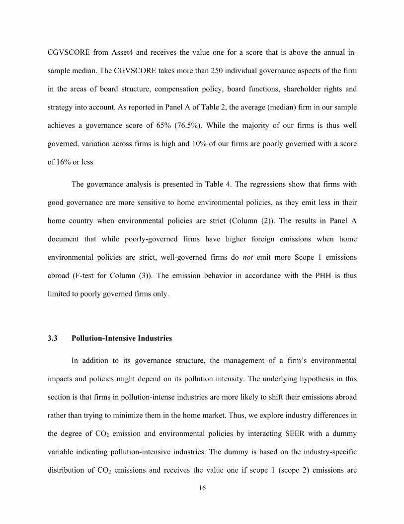
CGVSCORE from Asset4 and receives the value one for a score that is above the annual in-

sample median. The CGVSCORE takes more than 250 individual governance aspects of the firm

in the areas of board structure, compensation policy, board functions, shareholder rights and

strategy into account. As reported in Panel A of Table 2, the average (median) firm in our sample

achieves a governance score of 65% (76.5%). While the majority of our firms is thus well

governed, variation across firms is high and 10% of our firms are poorly governed with a score

of 16% or less.

The governance analysis is presented in Table 4. The regressions show that firms with

good governance are more sensitive to home environmental policies, as they emit less in their

home country when environmental policies are strict (Column (2)). The results in Panel A

document that while poorly-governed firms have higher foreign emissions when home

environmental policies are strict, well-governed firms do not emit more Scope 1 emissions

abroad (F-test for Column (3)). The emission behavior in accordance with the PHH is thus

limited to poorly governed firms only.

3.3 Pollution-Intensive Industries

In addition to its governance structure, the management of a firm’s environmental

impacts and policies might depend on its pollution intensity. The underlying hypothesis in this

section is that firms in pollution-intense industries are more likely to shift their emissions abroad

rather than trying to minimize them in the home market. Thus, we explore industry differences in

the degree of CO2 emission and environmental policies by interacting SEER with a dummy

variable indicating pollution-intensive industries. The dummy is based on the industry-specific

distribution of CO2 emissions and receives the value one if scope 1 (scope 2) emissions are

17

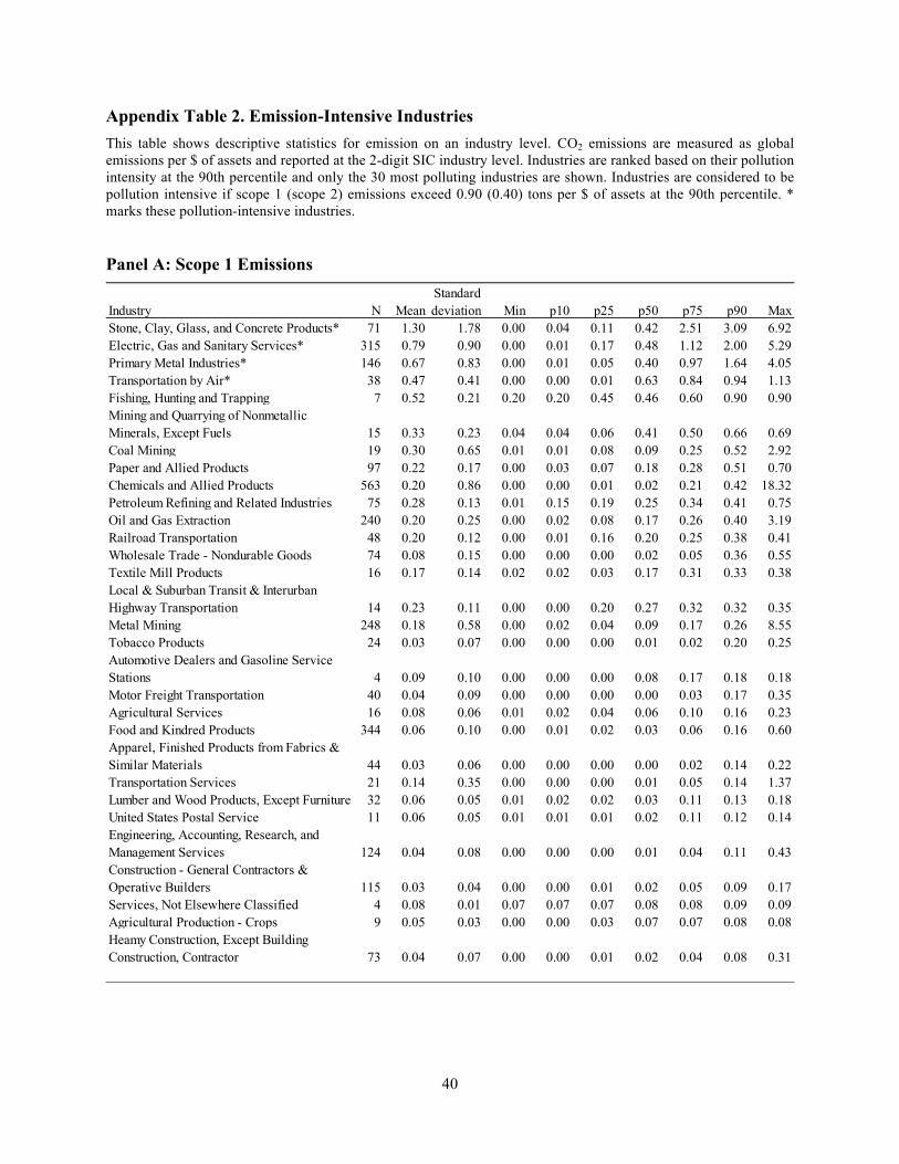
exceed 0.90 (0.40) tons per $ of assets at the 90th percentile. We thus define pollution-intensive

industries based on the level of emissions of the 10% most polluting firms in every industry. As

reported in Appendix Table 2, pollution-intensive industries in terms of scope 1 emissions are

Stone, Clay, Glass, and Concrete Products; Electric, Gas and Sanitary Services; Primary Metal

Industries; and Transportation by Air. In terms of scope 2 emissions, pollution-intensive

industries are Primary Metal Industries; Coal Mining; Metal Mining; and Mining and Quarrying

of Nonmetallic Minerals, Except Fuels.

The industry analysis is presented in Table 5. The regression results reveal that firms in

pollution-intensive industries act differently from firms in industries with more moderate

pollution intensity. The regressions in Panel A regarding scope 1 emissions reveal that when

environmental policies firms in pollution-moderate industries emit less at home while firms in

pollution-intensive industries do not (F-test for Column (2)). Furthermore, only firms in

pollution-intensive industries emit more abroad (Column (3)). Thus we conclude that with

respect to the firm’s direct emissions from operations, only firms in pollution-intensive industries

exhibit behavior in accordance with the PHH. The regressions regarding scope 2 emissions, e.g.

emissions from purchased electricity, are shown in Panel B of Table 5. Here, results indicate that

all firms exhibit emission behavior in accordance with the PHH but this behavior is intensified

for firms in pollution-intensive industries. For policy makers these results suggest that national

environmental regulation tends to be at least partially effective, e.g. when regulating scope 1

emissions of moderately polluting industries. But national environmental regulation is ineffective

where it is most needed: for pollution-intensive industries.

18

3.4 Alternative Specification: Gravity Model

Another possible specification is based on a gravity model. While in the previous

specification, our focus was the environmental policies at the home country, the gravity model

allows us to explicitly investigate in what way the “distance” between home- and foreign-

environmental policies is related to the location of emissions. We use the gravity model to test

the hypothesis that a firm’s tendency to transfer polluting activity to foreign countries increases

with the gap between the environmental policies in the home country relative to the foreign

country. Put differently, countries with less stringently enforced environmental policies “attract”

pollution from firms based in countries with very strict environmental policies.

Figure 3 provides an intuitive visualization of the gravity model approach to the PHH. In

this model, we focus on the emissions of firm i in foreign country c in year t. The variable of

interest is the spread between the SEER of the firm’s home country and the SEER in foreign

country c. On the x-axis, the left bars represent observations with stronger environmental

regulation abroad; the middle bars represent observations of similar environmental regulation at

home and abroad; and the right bars represent observations with stronger environmental

regulation at home. The y-axis shows tons of CO2 emissions per GDP of the foreign country,

which is averaged across all firm-country-year observations. Panel A includes all observations

for which SEER in the home and foreign country is known. Panel B includes only those

observations from firms with non-zero emissions in foreign country c in year t. The bars increase

from left to right, in especially in Panel B. This is in line with the PHH and indicate that firms

emit in those foreign countries where the gap in environmental regulation is most favorable for

them.

19

To implement the gravity model empirically, we pursue the following procedure. We

create a large matrix that has a cell for year firm-country-year combination (assuming that the

firm was in our database that year). In each cell, we record the pollution of the firm in the

country during the specific year. Importantly, we have a cell also for firm-country-years for

which there was no activity. In fact, about 95% of our dataset has zero activity. We drop

observations of firms with their home country, as our intention is to study the choice of country

of pollution.

Our variable of interest in the gravity model is the distance, or difference, between the

SEERHome and SEERForeign, (SEERHome - SEERForeign) which are the environmental policies score

for the home country and the foreign country, respectively. Positive (negative) values indicate

that the regulation is stronger (weaker) at home. The higher the value of SEER, the stronger the

regulation at home relative to the foreign country. Note that the home country is a firm

characteristic, while the foreign country changes from one cell to another.

The results of the gravity model are in Table 6. In the regressions, we regress either the

logged CO2 emission (in tons) or the percentage of global emissions that the firm emits in the

foreign country. On the right-hand side, our main variable is the difference in the SEER scores

between the home and foreign country. As before, we control for logged firm assets, and the

share in foreign assets. In addition, we control for the foreign country’s GDP, as well as controls

that reflect the relations between the home and foreign countries: logged geographic distance (in

kilometers), whether the countries share a common border, and whether the countries share

colonial history. We also include year, industry, foreign country, and home country fixed effects.

In all regressions of Table 6, we estimate a positive coefficient for SEER. These results

indicate that foreign emissions are higher in countries where environmental regulation is weaker

20

relative to the firm’s home country. This finding is consistent with the PHH, which postulates

that firms export pollution to countries where environmental regulation is relatively weaker.

The other control variables have the expected signs: Emissions are higher for larger, more

international firms, and when countries are geographically closer, trade more with each other, or

have a colonial history. The more internationally a firm operates, the higher its foreign

emissions. These results make intuitive sense considering that emissions are the direct result of a

firm’s production or operations.

3.5 Additional tests and robustness checks

3.5.1 The influence of stringency and enforcement of environmental regulation

Since our measure of a country’s quality of environmental regulation rests on both the

stringency and enforcement thereof, we also investigate whether our findings are driven by either

the stringency or the enforcement of environmental regulation at home, or both. In Appendix

Table 3, we address this issue and separate SEER into its two components SER (stringency of

environmental regulation) and EER (enforcement of environmental regulation). In Panels A and

B, we investigate the individual effects of SER and EER on firms’ emission levels for Scope 1

and Scope 2 emissions, respectively. Our results show that individually, both the stringency of

environmental regulation and the enforcement of this regulation significantly affects the

emission levels in the same ways.

In Panels C and D of Appendix Table 3 we go one step further and investigate the

simultaneous effects of SER and EER on the emission levels. To do so, we orthogonalize EER in

our regression specifications. The results of this exercise are as follows. While the stringency of

21

environmental regulation, SER, negatively affects overall and home emission levels, it affects

positively the absolute and relative foreign emission levels. These results are consistent with our

previously documented findings. Similarly, the enforcement of environmental regulation, EER,

significantly affects home and foreign emission levels above and beyond SER with the exception

of foreign scope 2 emissions which just miss the 10% significance level (columns (3) in Panel

D). This implies that enforcement and stringency of environmental regulation are

complementary in shaping firm’s pollution behavior.

3.5.2 Addressing the self-reporting bias

The underlying information from CDP on emissions is self-reported in nature. This raises

concerns regarding a self-reporting bias in our data. To address this concern, we conducted a

sub-sample analysis similar to our main analysis in Table 3. This time, however, we only focus

on those firms which have their CO2 emissions externally verified. In doing so, we are able to

rule out the potential effects on our findings that a self-reporting bias might have. The findings of

this subsample analysis are in Appendix Table 4. The results are generally consistent to our main

results in Table 3: SEER has a negative effect on the global and home emission levels and a

positive relation with foreign emissions (both absolute and relative). This implies that for firms

that have their reported emissions externally verified, more stringently enforced environmental

regulations in the home market lead to lower emissions at home, but to higher emissions abroad.

22

4 Conclusion

Pollution is an undesired externality of manufacturing activity that is costly to avoid. As a

result, firms are likely to find ways to circumvent costly CO2 pollution abatement techniques.

One of those means could be to transfer manufacturing activities, which cause CO2, to countries,

where the environmental regulation is less stringently enforced as compared to the company’s

home market. As such, the argument goes that countries are also competing in an international

marketplace for industrial activity. Therefore, countries with relatively loosely defined and

enforced environmental legislation might use this characteristic to attract industrial activities, to

boost GDP and employment statistics. The combination of these demand and supply factors

results in the so-called Pollution Haven Hypothesis, which states that firms move their

production activities into countries where the enforcement of environmental regulation causes

lower pollution abatement costs, relative to the home country.

Our paper sheds light on this hypothesis using a novel dataset, which is comprised of

firm-level CO2 emissions data. We find evidence in favor of the Pollution Haven Hypothesis.

More specifically, we find that companies indeed shift their CO2 emitting activities into countries

where environmental regulation is less far developed and less stringently enforced: Scope 1 and

Scope 2 CO2 emission levels are significantly higher abroad if the environmental regulation in

the home market is more stringently enforced than abroad. These results hold in a standard firm-

level framework, as well as in a gravity model context.

Our paper has important implications for firms and countries alike. We document that

regulatory arbitrage takes place – firms move their CO2 intensive activities abroad, where

environmental regulation is less strict as compared to the home market. This implies that in order

to effectively combat pollution and climate change, a concerted action between countries is

23

needed so that the overall CO2 balance will not increase. The Paris Agreement on climate change

in 2015 was one important step towards achieving this goal. If no concerted effort is undertaken

to climate change, major stakeholders, such as large firms, will find ways to circumvent strict

environmental regulations in certain parts of the world and move their production activities

elsewhere.

For multinational firms with production facilities all around the globe, our results imply

that—depending on how quickly and effectively the Paris Agreement will be implemented by

countries—they still might have either the potential to benefit from the regulatory arbitrage

opportunities or should be prepared to invest in pollution abatement methods and techniques. It

remains to be seen if the Paris Agreement will harmonize national environmental regulation to

such an extent so that firms will have no incentive anymore to choose locations of operations

purely based on concerns about the strictness of environmental regulation in a particular country.

24

References

Aliyu, M. A. 2005. Foreign Direct Investment and the Environment: Pollution Haven Hypothesis Revisited. Working Paper, Eight Annual Conference on Global Economic Analysis, Lübeck, Germany.

Becker, R. A., and J. V. Henderson. 2000. Effects of Air Quality Regulations on Polluting Industries. Journal of Political Economy 108(2), 379-421.

Becker, R. A., and J. V. Henderson. 2001. Costs of Air Quality Regulation. In: Carraro, C. and G. E. Metcalf (eds). 2001. Behavioral and Distributional Effects of Environmental Policy. University of Chicago Press, 159-186.

Ben Kheder, S. and N. Zugravu. 2012. Environmental Regulation and French Firms Location Abroad: An Economic Geography Model in an International Comparative Study. Ecological Economics 77, 48-61.

Bommer, R. 1999. Environmental Policy and Industrial Competitiveness: The Pollution-Haven Hypothesis Reconsidered. Review of International Economics 7(2), 342-355.

CDP. 2017. CDP – Driving Sustainable Economies. Retrieved from http://www.cdp.net. Accessed 24 June 2017.

Cole, M. A. 2004. Trade, the Pollution Haven Hypothesis and the Environmental Kuznets Curve: Examining the Linkages. Ecological Economics 48(1), 71-81.

Cole, M. A. and R. J. R. Elliott. 2005. FDI and the Capital Intensity of “Dirty” Sectors: A Missing Piece of the Pollution Haven Puzzle. Review of Development Economics 9(4), 530-548.

Dam, L. and B. Scholtens. 2012. The Curse of the Haven: The Impact of Multinational Enterprise on Environmental Regulation. Ecological Economics 78, 148-156.

Ederington, J., A. Levinson, and J. Minier. 2005. Footloose and Pollution-Free, Review of Economics and Statistics 87(1), 92–99.

Eskeland, G. S. and A. E. Harrison. 2003. Moving to Greener Pastures? Multinationals and the Pollution Haven Hypothesis. Journal of Development Economics 70(1), 1-23.

Esty, D. C. and M. E. Porter. 2005. National Environmental Performance: An Empirical Analysis of Policy Results and Determinants. Environment and Development Economics 10(4), 391-434.

Glick, R. and A. K. Rose. 2016. Currency Unions and Trade: A Post-EMU Reassessment. European Economic Review 87, 78-91.

25

Grossman, G. M. and A. B. Krueger. 1995. Economic Environment and the Economic Growth. Quarterly Journal of Economics 110(2), 353-377.

Kalamova, M. and N. Johnstone. 2011. Environmental Policy Stringency and Foreign Direct Investment. OECD Environment Working Papers, No. 33, OECD Publishing.

Kearsley, A. and M. Riddel. 2010. A Further Inquiry into the Pollution Haven Hypothesis and the Environmental Kuznets Curve. Ecological Economics 69(4), 905-919.

Kellenberg, D. K. 2009. An Empirical Investigation of the Pollution Haven Effect with Strategic Environment and Trade Policy. Journal of International Economics 78(2), 242-255.

Kleimeier, S. and M. Viehs. 2016. Carbon Disclosure, Emission Levels, and the Cost of Debt. Working Paper: Maastricht University.

Levinson, A. and M. S. Taylor. 2008. Unmasking the Pollution Haven Effect. International Economic Review 49(1), 223-254.

List, J. A. 2001. US County-Level Determinants of Inbound FDI: Evidence from a Two-Step Modified Count Data Model. International Journal of Industrial Organization 19(6), 953-973.

Leonard, H. J. and C. J. Duerksen. 1980. Environmental Regulations and the Location of Industry: An International Perspective. Columbia Journal of World Business, Summer, 52-68.

MacDermott, R. 2009. A Panel Study of the Pollution-Haven Hypothesis. Global Economy Journal 9(1).

Millimet, Daniel L. and John A. List. 2004. The Case of the Missing Pollution Haven Hypothesis, Journal of Regulatory Economics 26(3), 239–262.

Mulatu, A., R. Gerlagh, D. Rigby and A. Wossink. 2010. Environmental Regulation and Industry Location in Europe. Environmental and Resource Economics 45(4), 459-479.

Peters, G. P., G. Marland, C. Le Quéré, T. Boden, J. G. Canadell, and M. R. Raupach. (2012). Rapid Growth in CO2 Emissions after the 2008-2009 Global Financial Crisis. Nature Climate Change 2(1), 2-4.

Rajan, R. G. and L. Zingales. 1998. Financial Dependence and Growth. American Economic Review 88(3), 559-586.

Sen, S. 2015. Corporate Governance, Environmental Regulations, and Technological Change. European Economic Review 80, 36-61.

26

Shafik, N. and S. Bandyopadhyay. 1992. Economic Growth and Environmental Quality: Time-Series and Cross-Country Evidence. World Bank Publications, 904.

Socolow, R., 2006, Stabilization Wedges: An Elaboration of the Concept, in eds. H. J. Schellnhuber, W. Cramer, N. Nakicenovic, T. Wigley, and G. Yohe, Avoiding Dangerous Climate Change, Cambridge University Press.

Taylor, M. S. 2005. Unbundling the Pollution Haven Hypothesis. Advances in Economic Analysis & Policy 3(2).

Wagner, U. J. and C. D. Timmins. 2009. Agglomeration Effects in Foreign Direct Investment and the Pollution Haven Hypothesis. Environmental and Resource Economics 43(2), 231-256.

Walter, I. 1982. Environmentally Induced Industrial Relocation to Developing Countries, in R. J. Rubin and T.R. Graham (eds.) Environment and Trade. Allanheld, Osmun: Totowa, NJ.

27

Table 1. Summary Statistics The table shows descriptive statistics for all firms that report at least 85% of their global emissions on a country level and that have their headquarters in countries with environmental regulation data. Overall, 1,813 firms from 48 different home countries report Scope 1 emissions and 1,863 firms from 47 different home countries report Scope 2 emissions. Our proxy of environmental regulation (SEER) combines the World Economic Forum’s assessment of a country’s stringency and enforcement of environmental regulation. The proxy ranges from 0 to 7, with higher values indicating stricter environmental regulation.

Panel A: Scope 1 Emissions

Panel B: Scope 2 Emissions

YearNumber of firms

Firm's global emissions in

metric tons

Firm's emissions in home country

in % of firm's total global

emissions

Number of countries in

which firm has emissions

Environmental regulation

(SEER) in firm's home country

2008 573 5,004,705 71.9 6.0 3.92009 792 3,110,120 73.2 6.0 4.02010 734 3,119,675 61.4 8.1 4.12011 807 3,059,106 61.5 8.2 4.12012 855 3,145,869 58.8 8.6 4.22013 883 2,990,603 59.1 9.1 4.12014 1,030 2,724,609 56.8 9.0 4.22015 1,054 2,623,531 56.5 9.0 4.1

Average across firms

YearNumber of firms

Firm's global emissions in

metric tons

Firm's emissions in home country

in % of firm's total global

emissions

Number of countries in

which firm has emissions

Environmental regulation

(SEER) in firm's home country

2008 543 925,672 69.4 6.8 4.02009 812 740,259 69.9 6.9 4.02010 756 687,451 58.3 9.5 4.12011 834 654,047 57.1 9.9 4.12012 901 685,918 53.7 10.2 4.22013 918 728,495 53.3 10.7 4.12014 1,083 526,509 52.4 10.6 4.12015 1,100 521,705 52.6 10.6 4.1

Average across firms

28

Table 1. Summary Statistics (Cont.) Panel C: Stringency and enforcement of environmental regulation (SEER)

N = 150 Average Min Median Max Top 50 Mid 50 Bottom 502008 2.300 1.270 0.054 1.940 5.588 3.802 1.955 1.1352009 2.348 1.323 0.124 1.902 5.761 3.921 1.939 1.1752010 2.327 1.321 0.223 1.845 6.041 3.860 1.877 1.2342011 2.344 1.320 0.270 1.940 5.936 3.860 1.915 1.2582012 2.358 1.296 0.296 1.971 5.853 3.833 1.957 1.2762013 2.416 1.255 0.520 2.030 5.589 3.827 2.026 1.3862014 2.465 1.243 0.372 2.150 5.651 3.854 2.036 1.4962015 2.439 1.225 0.104 2.131 5.560 3.790 2.014 1.506

Average across… (2008)Standard deviation

29

Table 2. Descriptive Statistics The table presents descriptive statistics for our CO2 variables, the stringency and enforcement of environmental regulation (SEER) variable as well as specific firm-level variables which are used in the empirical analyses that follow.

Panel A: Sample of Firm-Level Observations

N MeanStandard devision Min p10 p25 p50 p75 p90 Max

Scope 1 CO 2 emissionsGlobal emissions ('000 tons) 6,325 3,149.84 13,693.48 0.00 2.42 12.58 88.81 585.23 4,500.00 183,400.00Home emissions ('000 tons) 6,325 1,846.21 8,813.60 0.00 0.37 3.76 33.89 307.34 2,700.00 180,000.00Foreign emissions ('000 tons) 6,325 1,303.63 8,487.66 0.00 0.00 0.95 13.28 148.91 1,151.05 175,571.07

ln(Global emissions) (tons) 6,325 11.43 2.92 0.18 7.79 9.44 11.39 13.28 15.32 19.03ln(Home emissions) (tons) 6,325 10.21 3.73 0.00 5.90 8.23 10.43 12.64 14.81 19.01ln(Foreign emissions) (tons) 6,325 8.88 4.41 0.00 0.00 6.86 9.49 11.91 13.96 18.98

Foreign emissions (% of global emissions) 6,325 38.30 34.68 0.00 0.00 4.97 30.23 68.28 94.72 100.00

Scope 2 CO 2 emissionsGlobal emissions ('000 tons) 6,530 678.94 2,683.42 0.00 6.91 33.10 136.04 493.02 1,500.27 120,000.00Home emissions ('000 tons) 6,530 374.62 2,069.16 0.00 0.75 7.75 49.23 241.38 882.79 120,000.00Foreign emissions ('000 tons) 6,530 304.31 1,541.90 0.00 0.00 2.86 27.43 168.85 594.51 75,300.00

ln(Global emissions) (tons) 6,530 11.65 2.14 0.91 8.84 10.41 11.82 13.11 14.22 18.60ln(Home emissions) (tons) 6,530 10.30 3.17 0.00 6.62 8.96 10.80 12.39 13.69 18.60ln(Foreign emissions) (tons) 6,530 9.26 4.05 0.00 0.00 7.96 10.22 12.04 13.30 18.14

Foreign emissions (% of global emissions) 6,530 42.83 35.78 0.00 0.00 7.51 37.52 77.53 96.58 100.00

Environmental regulation in firm's home countrySEER (0-7) 7,016 4.11 0.90 1.07 2.81 3.78 4.00 4.86 5.31 6.04SER (0-7) 7,016 5.43 0.56 2.90 4.68 5.20 5.38 5.91 6.13 6.63EER (0-7) 7,016 5.23 0.68 2.58 4.20 5.07 5.23 5.76 6.05 6.41

Firm characteristicsAssets ($m) 7,016 60.70 194.00 0.31 1.33 3.34 8.83 27.30 103.97 1,485.05ln(assets) ($m) 7,016 2.33 1.71 -2.12 0.29 1.21 2.18 3.31 4.64 6.87Foreign asset share (%) 5,417 26.40 26.15 0.00 0.00 4.41 17.54 43.71 66.73 98.77Corporate governance (0-100) 6,086 65.07 28.11 1.55 15.77 45.02 76.53 87.77 92.78 97.67

Home country characteristicsGDP ($bn) 7,016 5,384.21 6,106.45 19.56 386.40 1,055.00 2,646.00 6,157.00 16,160.00 18,040.00ln(GDP) ($m) 7,016 14.75 1.33 9.88 12.86 13.87 14.79 15.63 16.60 16.71GDP per capita growth (%) 7,016 0.64 2.43 -9.00 -2.91 -0.02 0.93 1.68 2.30 25.56

30

Table 2. Descriptive Statistics (Cont.) Panel B: Sample of Firm-Country-Level Observations Used in Gravity Analysis

N MeanStandard devision Min p10 p25 p50 p75 p90 Max

Scope 1 CO 2 emissions Foreign CO2 emissions ('000 tons) 671,717 8.75 319.98 0.00 0.00 0.00 0.00 0.00 0.00 66,000.00ln(Foreign CO2 emissions) (tons) 671,717 0.37 1.75 0.00 0.00 0.00 0.00 0.00 0.00 18.01Foreign CO2 emissions (% of global emissions) 671,717 0.27 2.90 0.00 0.00 0.00 0.00 0.00 0.00 100.00

Scope 2 CO2 emissions Foreign CO2 emissions ('000 tons) 689,448 2.23 70.23 0.00 0.00 0.00 0.00 0.00 0.00 14,000.00ln(Foreign CO2 emissions) (tons) 689,448 0.44 1.85 0.00 0.00 0.00 0.00 0.00 0.00 16.45Foreign CO2 emissions (% of global emissions) 689,448 0.31 3.15 0.00 0.00 0.00 0.00 0.00 0.00 100.00

Environmental regulationSEERhome - SEERforeign 744,782 1.80 1.52 -4.26 -0.42 0.88 2.04 2.84 3.60 5.67

Firm characteristicsAssets ($m) 744,782 51.05 146.77 0.12 1.35 3.34 8.79 26.94 89.42 960.47ln(Assets) ($m) 744,782 2.32 1.66 -2.12 0.30 1.21 2.17 3.29 4.49 6.87Foreign asset share (%) 744,782 26.46 26.14 0.00 0.00 4.34 17.81 44.04 66.63 98.77

Foreign country characteristicsGDP ($bn) 744,782 462.94 1,519.03 0.69 6.20 13.97 52.91 292.70 926.60 18,039.99ln(GDP) ($m) 744,782 11.13 1.98 6.54 8.73 9.54 10.88 12.59 13.74 16.71

Country pair characteristicsGeographic distance ('000 km) 744,782 8.20 4.09 0.14 2.26 5.14 8.40 10.80 13.83 19.89ln(Geographic distance) (km) 744,782 8.82 0.73 4.95 7.72 8.54 9.04 9.29 9.53 9.90Common border (0/1) 744,782 0.01 0.12 0.00 0.00 0.00 0.00 0.00 0.00 1.00Common colonial history (0/1) 744,782 0.05 0.22 0.00 0.00 0.00 0.00 0.00 0.00 1.00Trade ($bn) 744782 11.4 47.28 0 0.02 0.09 0.66 4.72 22.54 660.22ln(Trade) ($) 744,782 20.21 2.82 5.75 16.54 18.29 20.31 22.28 23.84 27.22

31

Table 3. Analysis of Firm-Level Emissions The table presents evidence about the relation between emissions in foreign countries and home-country environmental policies. Panels A and B show Scope 1 and 2 emissions, respectively. Columns (1) and (2) are estimated with ordinary least squares, and Columns (3) to (8) are estimated as a Tobit model. Standard errors are clustered by firm. SEER is our proxy of stringency and enforcement of environmental regulation in the firm’s home country, with higher values indicating stricter regulation. For each independent variable, the top row shows the estimated coefficient and the bottom row shows the t-statistic. ***, **, and * indicate significance at the 1%, 5%, and 10% level, respectively.


Dependent variable:

Specification:

SEER -0.18 *** -0.15 *** -0.38 *** -0.30 *** 0.40 *** 0.28 ** 4.54 *** 3.31 ***(-3.56) (-2.66) (-4.21) (-2.82) (3.84) (2.47) (4.06) (2.81)

Firm characteristicsln(Assets) 1.03 *** 1.05 *** 1.00 *** 1.07 *** 1.43 *** 1.30 *** 3.83 *** 1.82 **

(28.03) (27.01) (15.79) (15.87) (19.33) (18.16) (4.94) (2.51)Foreign asset share 0.00 -0.03 *** 0.04 *** 0.62 ***

(0.34) (-7.30) (11.87) (16.71)Home country characteristics

ln(GDP) 0.03 0.01 0.44 *** 0.32 *** -0.43 *** -0.19 ** -8.38 *** -5.16 ***(0.76) (0.30) (6.24) (3.97) (-5.86) (-2.50) (-10.90) (-6.36)

GDP per capita growth 0.01 0.00 0.05 0.03 -0.20 *** -0.15 *** -1.77 *** -1.23 ***(0.77) (0.28) (1.60) (0.80) (-4.86) (-3.73) (-4.33) (-3.20)

Fixed effectsYear yes yes yes yes yes yes yes yesIndustry yes yes yes yes yes yes yes yes

Adjusted/Pseudo R-squared 0.703 0.692 0.108 0.112 0.091 0.104 0.030 0.052Observations 6,325 4,919 6,325 4,919 6,325 4,919 6,325 4,919of which censored at 0 274 226 719 481 719 481of which censored at 100 274 226

OLS

ln(Global emissions (tons))

Foreign emissions in % of global emissions

OLS Tobit Tobit Tobit Tobit Tobit Tobit

ln(Home emissions (tons))

ln(Foreign emissions (tons))

(2) (3) (4) (5) (6) (7) (8)(1)

32

Table 3. Analysis of Firm-Level Emissions (Cont.) Panel B: Scope 2 Emissions

Dependent variable:

Specification:

SEER -0.20 *** -0.18 *** -0.48 *** -0.42 *** 0.41 *** 0.34 *** 7.38 *** 6.67 ***(-5.07) (-4.19) (-5.72) (-4.29) (4.25) (3.47) (6.90) (5.97)

Firm characteristicsln(Assets) 0.92 *** 0.93 *** 0.80 *** 0.87 *** 1.31 *** 1.21 *** 4.36 *** 2.53 ***

(29.81) (27.96) (14.33) (14.47) (19.79) (19.16) (5.96) (3.73)Foreign asset share -0.00 -0.03 *** 0.04 *** 0.61 ***

(-1.41) (-8.16) (11.20) (17.79)Home country characteristics

ln(GDP) 0.08 *** 0.06 ** 0.52 *** 0.40 *** -0.29 *** -0.11 * -8.50 *** -5.40 ***(2.76) (2.05) (7.88) (5.50) (-4.50) (-1.71) (-11.25) (-6.90)




Tobit





(6) (7) (8)OLS OLS Tobit Tobit Tobit Tobit Tobit(1) (2) (3) (4) (5)

33

Table 4. Environmental Regulation and Firm’s Corporate Governance The table shows results estimated as OLS (Column 1) and Tobit (Columns 2-4) regressions with standard errors clustered by country-pair. For each independent variable, the top row shows the estimated coefficient and the bottom row shows the t-statistic. The F-test assesses the joint significance of the coefficients of SEER and its interaction effect. ***, **, and * indicate significance at the 1%, 5%, and 10% level, respectively.


Dependent variable:

Specification:

SEER -0.14 ** -0.22 * 0.41 *** 3.45 **(-2.11) (-1.94) (2.76) (2.47)

SEER*I(Good governance) 0.00 -0.69 ** -0.36 * 4.67 *(0.01) (-2.46) (-1.68) (1.90)

Firm characteristicsln(Assets) 1.03 *** 1.07 *** 1.23 *** 1.56 **

(23.20) (14.33) (15.28) (2.02)Foreign asset share 0.00 -0.03 *** 0.04 *** 0.61 ***

(0.71) (-6.82) (10.77) (15.46)Good governanceD 0.09 2.54 ** 2.26 ** -10.07

(0.18) (2.23) (2.45) (-0.99)Home country characteristics

ln(GDP) 0.01 0.37 *** -0.29 *** -6.19 ***(0.32) (4.05) (-3.61) (-7.29)

GDP per capita growth 0.00 0.02 -0.12 *** -0.91 **(0.10) (0.54) (-3.22) (-2.39)

Fixed effectsYear yes yes yes yesIndustry yes yes yes yes

F-test 1.54 10.17 *** 0.08 12.04 ***

Adjusted/Pseudo R-squared 0.692 0.113 0.106 0.055Observations 4,376 4,376 4,376 4,376of which censored at 0 196 406 406of which censored at 100 196

OLS(3) (4)

ln(Global emissions

(tons))

ln(Home emissions

(tons))

ln(Foreign emissions

(tons))


(1)Tobit Tobit Tobit

(2)

34

Table 4. Environmental Regulation and Firm’s Corporate Governance (Cont.) Panel B: Scope 2 Emissions

Dependent variable:

Specification:

SEER -0.16 *** -0.37 *** 0.39 *** 6.53 ***(-3.05) (-3.69) (3.03) (4.95)

SEER*I(Good governance) -0.03 -0.53 * -0.22 4.33 *(-0.34) (-1.73) (-1.21) (1.71)

Firm characteristicsln(Assets) 0.91 *** 0.81 *** 1.16 *** 2.75 ***

(24.33) (12.44) (15.88) (3.72)Foreign asset share -0.00 ** -0.03 *** 0.04 *** 0.60 ***

(-1.99) (-7.58) (9.75) (15.96)Good governanceD 0.14 1.82 1.44 * -11.99

(0.36) (1.45) (1.75) (-1.11)Home country characteristics

ln(GDP) 0.05 0.45 *** -0.19 ** -6.14 ***(1.39) (5.16) (-2.56) (-7.26)

GDP per capita growth 0.01 0.03 -0.11 *** -1.00 ***(0.87) (0.73) (-3.06) (-2.63)


F-test 5.21 ** 9.07 *** 1.27 21.61 ***


(1)

ln(Global emissions

(tons))

ln(Home emissions

(tons))


(tons))


(2) (3) (4)OLS Tobit Tobit Tobit

35

Table 5. Environmental Regulation and Pollution-Intensive Industries The table shows results estimated as OLS (Column 1) and Tobit (Columns 2-4) regressions with standard errors clustered by country-pair. For each independent variable, the top row shows the estimated coefficient and the bottom row shows the t-statistic. The F-test assesses the joint significance of the coefficients of SEER and its interaction effect. ***, **, and * indicate significance at the 1%, 5%, and 10% level, respectively.


Dependent variable:

Specification:

SEER -0.15 *** -0.32 *** 0.17 3.06 **(-2.60) (-2.74) (1.51) (2.41)

SEER*I(Pollution-intensive industry) 0.02 0.17 0.94 ** 2.20(0.09) (0.67) (2.04) (0.69)




ln(GDP) 0.01 0.32 *** -0.19 ** -5.16 ***(0.30) (3.96) (-2.55) (-6.37)



F-test 0.46 0.47 6.19 ** 3.23 *


OLS Tobit Tobit Tobit(1) (2) (3)

ln(Global emissions

(tons))

ln(Home emissions

(tons))


(tons))


(4)

36

Table 5. Environmental Regulation and Pollution-Intensive Industries (Cont.) Panel B: Scope 2 Emissions

Dependent variable:

Specification:

SEER -0.18 *** -0.35 *** 0.27 *** 5.64 ***(-4.26) (-3.65) (2.73) (5.00)

SEER*I(Pollution-intensive industry) 0.02 -1.15 * 1.16 ** 17.68 ***(0.09) (-1.96) (2.31) (3.35)


(27.96) (14.53) (19.36) (3.78)Foreign asset share -0.00 -0.03 *** 0.04 *** 0.61 ***


ln(GDP) 0.06 ** 0.41 *** -0.12 * -5.52 ***(2.04) (5.65) (-1.84) (-7.13)



F-test 0.35 6.64 *** 8.47 *** 20.47 ***


(1) (2) (3) (4)OLS Tobit Tobit Tobit

ln(Global emissions

(tons))

ln(Home emissions

(tons))


(tons))


37

Table 6. Gravity Model The table shows gravity model results estimated as Tobit regressions with standard errors clustered by country-pair. SEERdiff is our proxy of stringency and enforcement of environmental regulation in the home minus the foreign country, with higher values indicating stricter regulation at home. For each independent variable, the top row shows the estimated coefficient and the bottom row shows the t-statistic. ***, **, and * indicate significance at the 1%, 5%, and 10% level, respectively.

Dependent variable:

Specification:

SEERhome - SEERforeign 0.40 *** 0.52 *** 0.38 *** 0.39 **(2.93) (2.93) (3.00) (2.44)

Controls - firm characteristicsln(Assets) 2.38 *** 2.29 *** 1.96 *** 1.88 ***

(32.79) (16.92) (31.20) (14.27)Foreign asset share 0.05 *** 0.07 *** 0.04 *** 0.05 ***

(16.82) (11.79) (14.02) (9.58)Controls - foreign country characteristics

ln(GDP) -0.51 -0.67 0.49 0.61(-1.38) (-1.39) (1.44) (1.30)

Gravity controls - country pair characteristicsln(Geographic distance) -1.67 *** -2.16 *** -1.33 *** -1.83 ***

(-5.49) (-4.99) (-4.99) (-4.41)Common border 0.80 2.18 * 0.67 1.75

(1.14) (1.86) (1.06) (1.44)Common colonial history 3.04 *** 4.42 *** 2.97 *** 4.46 ***

(6.38) (6.38) (7.42) (6.60)ln(Trade) 1.93 *** 2.52 *** 1.86 *** 2.44 ***

(10.02) (8.53) (10.72) (8.93)Fixed effects

Year yes yes yes yesIndustry yes yes yes yesForeign country yes yes yes yesHome country yes yes yes yes

Pseudo R-squared 0.198 0.178 0.203 0.183Observations 671,717 671,717 689,448 689,448of which censored at 0 636,406 636,406 645,856 645,856of which uncensored 35,311 35,296 43,592 43,573of which censored at 100 15 19

Scope 1 emissions Scope 2 emissions


(tons))



(tons))


(1) (2) (3) (4)Tobit Tobit Tobit Tobit

38

Appendix Table 1. Variable Definitions and Sources Panel A: Variables used in firm-level analysis

Variable Description Units Original Data SourceDependent variables

Global emissions (tons)

firm i's CO2 emissions globally in year t, calculated for either scope 1 or scope 2 emissions

tons CDP

Home emissions (tons)

firm i's CO2 emissions in home country in year t, calculated for either scope 1 or scope 2 emissions

tons CDP

Foreign emissions (tons)

firm i's CO2 emissions in all foreign countries combined in year t, calculated for either scope 1 or scope 2 emissions

tons CDP


firm i's CO2 emissions in all foreign countries combined in year t in percent of firm i's global CO2 emissions in year t, calculated for either scope 1 or scope 2 emissions

0-100 with 1.0=1%

CDP

Independent variablesSER stringency of environmental regulation in firm i's home country in

year t0-7 World Economic Forum

EER enforcement of environmental regulation in firm i's home country in year t

0-7 World Economic Forum

SEER stringency and enforcement of environmental regulation in firm i's home country in year t; calculated as SEER = (SER*EER)/7

0-7 World Economic Forum

Assets total assets of firm i in year t (WC02999) US$ million WorldscopeForeign asset share firm i's foreign assets in % of total assets in year t (WC08736) 0-100 with

1.0=1%Worldscope

Good governanceD dummy equal to 1 if firm i's corporate governance score in year t is larger than sample median, 0 otherwise

0/1 Asset4

Pollution-intensive industryD

dummy equal to 1 if firm belongs to pollution-intensive industries, 0 otherwise; industries are considered to be pollution intensive if scope 1 (scope 2) emissions exceed 0.90 (0.40) tons per $ of assets at the 90th percentile

0/1 CDP, Worldscope

External verificationD dummy equal to 1 if firm i's emissions in year t are externally verified, 0 otherwise

0/1 CDP

GDP gross domestic product in firm i's home country in year t current US$ million

World Bank's World Development Indicators

GDP per capita growth

annual percentage growth rate of GDP per capita for firm i's home country in year t

0-100 with 1.0=1%


39

Appendix Table 1. Variable Definitions and Sources (Cont.) Panel B: Variables used in gravity analysis

Panel C: Fixed effects used in firm-level and gravity analyses

Variable Description Units Original Data SourceDependent variables

Foreign emissions (tons)

firm i's CO2 emissions in foreign country c in year t, calculated for either scope 1 or scope 2 emissions

tons CDP


firm i's CO2 emissions in foreign country c in year t in percent of firm i's global CO2 emissions in year t, calculated for either scope 1 or scope 2 emissions

0-100 with 1.0=1%

CDP

Independent variablesSEERhome-SEERforeign difference between stringency and enforcement of environmental

regulation in firm i's home country and foreign country c in year t; each country's SEER is calculated as SEER = (SER*EER)/7

-7 to +7 World Economic Forum

Assets total assets of firm i in year t (WC02999) US$ million WorldscopeForeign asset share firm i's foreign assets in % of total assets in year t (WC08736) 0-100 with

1.0=1%Worldscope

GDP gross domestic product in foreign country c in year t current US$ million


Geographic distance geographic distance between firm i's home country and foreign country c, measured using the great circle distance formula

km www.distancefromto. net

Common border dummy equal to 1 if firm i's home country and the foreign country c share a land border, 0 otherwise

0/1 Glick and Rose (2016), CIA World Factbook

Common colonial history

dummy equal to 1 if firm i's home country and foreign country c have a colonial history or belonged to same country

0/1 Glick and Rose (2016)

Trade sum of exports and imports between firm i's home country and foreign country c in year t

US$ IMF's Direction of Trade Statistics

Variable Description Units Original Data SourceYear dummies identifying the year t in which firm i emits CO2 0/1 CDPIndustry dummies based on 2-digit SIC codes (WC07021) 0/1 WorldscopeForeign country dummies identifying the foreign country c in which firm i emits CO2 0/1 CDPHome country dummies identifying the home country in which firm i is

headquartered0/1 CDP

40

Appendix Table 2. Emission-Intensive Industries This table shows descriptive statistics for emission on an industry level. CO2 emissions are measured as global emissions per $ of assets and reported at the 2-digit SIC industry level. Industries are ranked based on their pollution intensity at the 90th percentile and only the 30 most polluting industries are shown. Industries are considered to be pollution intensive if scope 1 (scope 2) emissions exceed 0.90 (0.40) tons per $ of assets at the 90th percentile. * marks these pollution-intensive industries.


Industry N MeanStandard deviation Min p10 p25 p50 p75 p90 Max

Stone, Clay, Glass, and Concrete Products* 71 1.30 1.78 0.00 0.04 0.11 0.42 2.51 3.09 6.92Electric, Gas and Sanitary Services* 315 0.79 0.90 0.00 0.01 0.17 0.48 1.12 2.00 5.29Primary Metal Industries* 146 0.67 0.83 0.00 0.01 0.05 0.40 0.97 1.64 4.05Transportation by Air* 38 0.47 0.41 0.00 0.00 0.01 0.63 0.84 0.94 1.13Fishing, Hunting and Trapping 7 0.52 0.21 0.20 0.20 0.45 0.46 0.60 0.90 0.90Mining and Quarrying of Nonmetallic Minerals, Except Fuels 15 0.33 0.23 0.04 0.04 0.06 0.41 0.50 0.66 0.69Coal Mining 19 0.30 0.65 0.01 0.01 0.08 0.09 0.25 0.52 2.92Paper and Allied Products 97 0.22 0.17 0.00 0.03 0.07 0.18 0.28 0.51 0.70Chemicals and Allied Products 563 0.20 0.86 0.00 0.00 0.01 0.02 0.21 0.42 18.32Petroleum Refining and Related Industries 75 0.28 0.13 0.01 0.15 0.19 0.25 0.34 0.41 0.75Oil and Gas Extraction 240 0.20 0.25 0.00 0.02 0.08 0.17 0.26 0.40 3.19Railroad Transportation 48 0.20 0.12 0.00 0.01 0.16 0.20 0.25 0.38 0.41Wholesale Trade - Nondurable Goods 74 0.08 0.15 0.00 0.00 0.00 0.02 0.05 0.36 0.55Textile Mill Products 16 0.17 0.14 0.02 0.02 0.03 0.17 0.31 0.33 0.38Local & Suburban Transit & Interurban Highway Transportation 14 0.23 0.11 0.00 0.00 0.20 0.27 0.32 0.32 0.35Metal Mining 248 0.18 0.58 0.00 0.02 0.04 0.09 0.17 0.26 8.55Tobacco Products 24 0.03 0.07 0.00 0.00 0.00 0.01 0.02 0.20 0.25Automotive Dealers and Gasoline Service Stations 4 0.09 0.10 0.00 0.00 0.00 0.08 0.17 0.18 0.18Motor Freight Transportation 40 0.04 0.09 0.00 0.00 0.00 0.00 0.03 0.17 0.35Agricultural Services 16 0.08 0.06 0.01 0.02 0.04 0.06 0.10 0.16 0.23Food and Kindred Products 344 0.06 0.10 0.00 0.01 0.02 0.03 0.06 0.16 0.60Apparel, Finished Products from Fabrics & Similar Materials 44 0.03 0.06 0.00 0.00 0.00 0.00 0.02 0.14 0.22Transportation Services 21 0.14 0.35 0.00 0.00 0.00 0.01 0.05 0.14 1.37Lumber and Wood Products, Except Furniture 32 0.06 0.05 0.01 0.02 0.02 0.03 0.11 0.13 0.18United States Postal Service 11 0.06 0.05 0.01 0.01 0.01 0.02 0.11 0.12 0.14Engineering, Accounting, Research, and Management Services 124 0.04 0.08 0.00 0.00 0.00 0.01 0.04 0.11 0.43Construction - General Contractors & Operative Builders 115 0.03 0.04 0.00 0.00 0.01 0.02 0.05 0.09 0.17Services, Not Elsewhere Classified 4 0.08 0.01 0.07 0.07 0.07 0.08 0.08 0.09 0.09Agricultural Production - Crops 9 0.05 0.03 0.00 0.00 0.03 0.07 0.07 0.08 0.08Heamy Construction, Except Building Construction, Contractor 73 0.04 0.07 0.00 0.00 0.01 0.02 0.04 0.08 0.31

41

Appendix Table 2. Emission-Intensive Industries (Cont.) Panel B: Scope 2 Emissions

Industry N MeanStandard deviation Min p10 p25 p50 p75 p90 Max

Primary Metal Industries* 137 0.18 0.25 0.00 0.02 0.05 0.08 0.19 0.65 1.16Coal Mining* 19 0.17 0.27 0.00 0.00 0.01 0.02 0.32 0.61 0.95Metal Mining* 247 0.16 0.20 0.00 0.01 0.02 0.06 0.23 0.47 0.93Mining and Quarrying of Nonmetallic Minerals, Except Fuels* 15 0.19 0.18 0.02 0.02 0.09 0.10 0.41 0.47 0.53Fishing, Hunting and Trapping 8 0.20 0.11 0.01 0.01 0.14 0.20 0.27 0.38 0.38Textile Mill Products 11 0.12 0.11 0.01 0.01 0.03 0.13 0.17 0.29 0.32Eating and Drinking Places 35 0.09 0.12 0.00 0.00 0.00 0.03 0.14 0.29 0.40Stone, Clay, Glass, and Concrete Products 60 0.22 0.40 0.00 0.04 0.08 0.14 0.19 0.23 2.02Paper and Allied Products 90 0.12 0.13 0.00 0.01 0.04 0.07 0.16 0.22 0.64Apparel and Accessory Stores 56 0.07 0.08 0.00 0.01 0.02 0.04 0.07 0.22 0.39Rubber and Miscellaneous Plastic Products 79 0.08 0.08 0.00 0.01 0.03 0.06 0.09 0.20 0.40Hotels, Rooming Houses, Camps, and Other Lodging Places 48 0.08 0.13 0.01 0.02 0.03 0.04 0.07 0.20 0.89Chemicals and Allied Products 544 0.11 0.88 0.00 0.00 0.01 0.03 0.11 0.18 20.47Fabricated Metal Products 76 0.06 0.07 0.00 0.01 0.02 0.03 0.10 0.14 0.34Electronic & Other Electrical Equipment & Components 502 0.08 0.40 0.00 0.01 0.01 0.04 0.08 0.14 8.91General Merchandise Stores 49 0.07 0.06 0.00 0.01 0.04 0.06 0.09 0.14 0.33Food Stores 85 0.08 0.07 0.00 0.02 0.04 0.07 0.11 0.13 0.54Agricultural Production - Crops 17 0.04 0.04 0.00 0.00 0.00 0.02 0.06 0.11 0.12Apparel, Finished Products from Fabrics & Similar Materials 44 0.03 0.04 0.00 0.00 0.01 0.02 0.04 0.11 0.14Food and Kindred Products 341 0.44 7.26 0.00 0.00 0.01 0.03 0.05 0.10 134.17Lumber and Wood Products, Except Furniture 34 0.07 0.09 0.01 0.01 0.02 0.03 0.09 0.10 0.34Health Services 15 0.04 0.04 0.00 0.01 0.02 0.03 0.04 0.10 0.15Petroleum Refining and Related Industries 83 0.04 0.06 0.00 0.00 0.01 0.02 0.05 0.09 0.29Railroad Transportation 46 0.02 0.04 0.00 0.00 0.01 0.01 0.02 0.09 0.16Furniture and Fixtures 32 0.04 0.04 0.01 0.01 0.01 0.03 0.06 0.08 0.17Building Materials, Hardware, Garden Supplies & Mobile Homes 31 0.04 0.03 0.00 0.01 0.01 0.05 0.07 0.08 0.08Miscellaneous Retail 46 0.04 0.05 0.00 0.00 0.01 0.02 0.06 0.08 0.21Construction - General Contractors & Operative Builders 117 0.03 0.09 0.00 0.00 0.00 0.01 0.02 0.07 0.82Local & Suburban Transit & Interurban Highway Transportation 14 0.06 0.10 0.01 0.02 0.02 0.03 0.05 0.07 0.41Amusement and Recreation Services 20 0.04 0.03 0.00 0.00 0.01 0.03 0.07 0.07 0.07

42

Appendix Table 3. SER vs. EER The table presents evidence about the relation between emissions in foreign countries and home-country stringency and enforcement (SER and EER) or environmental policies. Panels A, C and B, D show Scope 1 and 2 emissions, respectively. Columns (1) and (2) are estimated with ordinary least squares, and Columns (3) to (8) are estimated as a Tobit model. Standard errors are clustered by firm. For each independent variable, the top row shows the estimated coefficient and the bottom row shows the t-statistic. ***, **, and * indicate significance at the 1%, 5%, and 10% level, respectively.


Dependent variable:

Specification:

SER (stringency) -0.25 *** -0.47 *** 0.46 ** 5.25 ***(-2.71) (-2.62) (2.46) (2.73)

EER (enforcement) -0.19 *** -0.45 *** 0.44 *** 5.44 ***(-2.61) (-3.34) (2.87) (3.48)

Firm characteristicsln(Assets) 1.05 *** 1.05 *** 1.07 *** 1.07 *** 1.30 *** 1.31 *** 1.82 ** 1.84 **

(27.02) (26.97) (15.87) (15.86) (18.16) (18.20) (2.51) (2.55)Foreign asset share 0.00 0.00 -0.03 *** -0.03 *** 0.04 *** 0.04 *** 0.62 *** 0.62 ***

(0.33) (0.37) (-7.31) (-7.26) (11.87) (11.81) (16.72) (16.66)Home country characteristics

ln(GDP) 0.01 0.02 0.32 *** 0.34 *** -0.19 ** -0.20 *** -5.15 *** -5.34 ***(0.28) (0.47) (3.95) (4.20) (-2.48) (-2.71) (-6.34) (-6.62)





(4) (6) (8)(1) (2) (7)




OLS OLS Tobit Tobit Tobit(3) (5)

Tobit Tobit Tobit

43

Appendix Table 3. SER vs. EER (Cont.) Panel B: Scope 2 Emissions

Dependent variable:

Specification:

SER (stringency) -0.30 *** -0.65 *** 0.57 *** 10.50 ***(-4.38) (-3.98) (3.43) (5.79)

EER (enforcement) -0.23 *** -0.62 *** 0.50 *** 9.89 ***(-3.92) (-4.73) (3.80) (6.58)

Firm characteristicsln(Assets) 0.93 *** 0.93 *** 0.87 *** 0.87 *** 1.21 *** 1.21 *** 2.55 *** 2.56 ***

(27.96) (27.93) (14.45) (14.47) (19.17) (19.20) (3.74) (3.79)Foreign asset share -0.00 -0.00 -0.03 *** -0.03 *** 0.04 *** 0.04 *** 0.61 *** 0.60 ***

(-1.42) (-1.38) (-8.16) (-8.10) (11.20) (11.12) (17.78) (17.70)Home country characteristics

ln(GDP) 0.06 ** 0.07 ** 0.40 *** 0.43 *** -0.11 * -0.13 ** -5.38 *** -5.75 ***(2.02) (2.33) (5.45) (5.86) (-1.69) (-1.99) (-6.82) (-7.48)





(1) (3) (5)(2) (4) (6) (8)


(7)OLS OLS Tobit Tobit Tobit Tobit Tobit Tobit



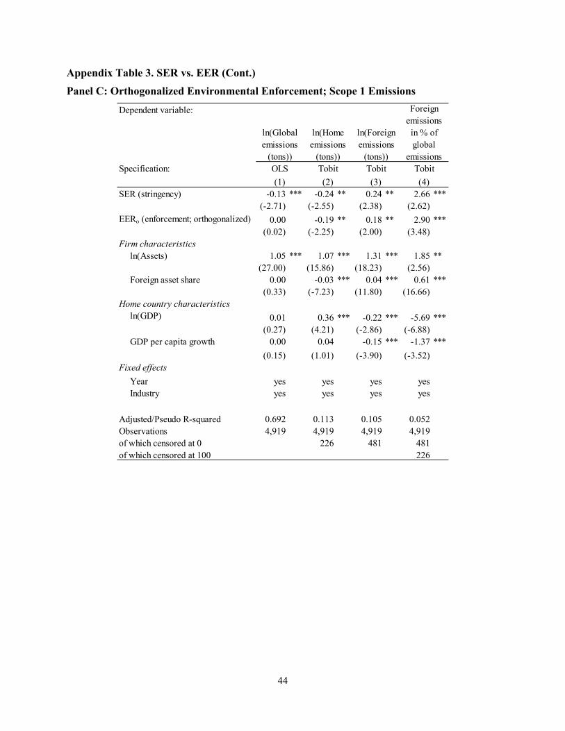
44

Appendix Table 3. SER vs. EER (Cont.) Panel C: Orthogonalized Environmental Enforcement; Scope 1 Emissions

Dependent variable:

Specification:

SER (stringency) -0.13 *** -0.24 ** 0.24 ** 2.66 ***(-2.71) (-2.55) (2.38) (2.62)

EERo (enforcement; orthogonalized) 0.00 -0.19 ** 0.18 ** 2.90 ***(0.02) (-2.25) (2.00) (3.48)




ln(GDP) 0.01 0.36 *** -0.22 *** -5.69 ***(0.27) (4.21) (-2.86) (-6.88)




OLS Tobit Tobit Tobit(4)(1) (2) (3)

ln(Global emissions

(tons))

ln(Home emissions

(tons))


(tons))

Foreign emissions in % of global

emissions

45

Appendix Table 3. SER vs. EER (Cont.) Panel D: Orthogonalized Environmental Enforcement; Scope 2 Emissions

Dependent variable:

Specification:

SER (stringency) -0.16 *** -0.33 *** 0.30 *** 5.41 ***(-4.40) (-3.92) (3.37) (5.74)

EERo (enforcement; orthogonalized) 0.01 -0.24 ** 0.12 3.62 ***(0.17) (-2.53) (1.61) (4.06)




ln(GDP) 0.06 * 0.45 *** -0.13 ** -6.08 ***(1.95) (5.91) (-1.97) (-7.74)




Tobit(4)(1) (2) (3)

ln(Global emissions

(tons))

ln(Home emissions

(tons))


(tons))

Foreign emissions in % of global

emissionsOLS Tobit Tobit

46

Appendix Table 4. Subsample Analysis – Only Externally Verified Emissions The table presents evidence about the relation between emissions in foreign countries and home-country environmental policies for companies which have their emission information externally verified. Panels A and B show Scope 1 and 2 emissions, respectively. Column (1) is estimated with ordinary least squares, and Columns (2) to (4) are estimated as a Tobit model. Standard errors are clustered by firm. SEER is our proxy of stringency and enforcement of environmental regulation in the firm’s home country, with higher values indicating stricter regulation. For each independent variable, the top row shows the estimated coefficient and the bottom row shows the t-statistic. ***, **, and * indicate significance at the 1%, 5%, and 10% level, respectively.


Dependent variable:

Specification:

SEER -0.16 ** -0.37 *** 0.28 ** 3.24 **(-2.55) (-3.28) (2.34) (2.55)


(24.23) (11.77) (15.71) (2.87)Foreign asset share 0.00 * -0.03 *** 0.04 *** 0.61 ***


ln(GDP) 0.04 0.34 *** -0.11 -5.01 ***(0.83) (3.90) (-1.33) (-5.50)




OLS Tobit Tobit Tobit(1) (2) (3) (4)

ln(Global emissions

(tons))

ln(Home emissions

(tons))


(tons))

Foreign emissions

in % of global

emissions

47

Appendix Table 4. Subsample Analysis – Only Externally Verified Emissions (Cont.) Panel B: Scope 2 Emissions

Dependent variable:

Specification:

SEER -0.15 *** -0.41 *** 0.32 *** 6.14 ***(-3.13) (-3.70) (3.03) (4.90)




ln(GDP) 0.04 0.44 *** -0.14 * -5.83 ***(1.13) (4.84) (-1.92) (-6.42)




OLS Tobit Tobit Tobit


(tons))

Foreign emissions

in % of global

emissions

(1) (2) (3) (4)

ln(Global emissions

(tons))

ln(Home emissions

(tons))

48

Figure 1. Global Development of Environmental Regulation The heat maps show our proxy of environmental regulation (SEER) for the 150 countries included in our sample. SEER combines the World Economic Forum’s assessment of a country’s stringency and enforcement of environmental regulation. SEER ranges from 0 to 7, with higher values indicating stricter environmental regulation.

Figure 1a. 2008

Figure 1b. 2015

49

Figure 2. Visualization of the Pollution Haven Hypothesis with Respect to Home-Country Environmental Regulation The figure visualizes the Pollution Haven Hypothesis (PHH) with respect to home-country environmental regulation. Environmental regulation is shown on the x axis and measured as SEER, which combines the World Economic Forum’s assessment of a country’s stringency and enforcement of environmental regulation. SEER ranges from 0 to 7, with higher values indicating stricter environmental regulation. The firm’s home-country emissions as a percentage of its global emissions are shown on the y axis. Each bubble pools firms according to their home-country SEER. The bubble size indicates tons of CO2 exported per million USD of assets for the average firm. This value is listed inside the bubble, together with the SEER range.

Figure 2a. Scope 1 Emissions

Figure 2b. Scope 2 Emissions

50

Figure 3. Differences in Environmental Regulation and Emissions in Foreign Countries The figure presents the differences in environmental regulation and emissions in foreign countries. Figure 3a includes all observations for which SEER in the home and foreign country is known. Figure 3b excludes all observations with zero emissions. The x-axis shows three categories for the difference in environmental regulation in the home versus foreign country. Higher values indicate stronger regulation at home. Thus, the left/middle/right bars reflect country pairs with stronger/similar/weaker regulation abroad. The y-axis shows average tons of CO2 emissions per million USD of foreign country GDP.

Figure 3a. Average Emissions

Figure 3b. Average Emissions Excluding Firms with Zero Emissions in a Given Foreign Country

20171207 writeup pollution...

Documents