2013 cayuga lake study technical briefing (cltac) … cayuga lake study technical briefing (cltac)...
TRANSCRIPT

2013 Cayuga Lake Study
Technical Briefing (CLTAC)
Cayuga Lake Modeling Project
Nov. 5, 2014
Nov. 5, 2014 Upstate Freshwater Institute 1

Outline1. Goals and Analysis Components
2. Monitoring
3. Constituent Concentrations
4. Concentration-Driver Relationships
5. Load Estimation Techniques and Best Methods
6. 2013 April – October Load Estimates
7. P bioavailability and Loads
8. 2000-2012, Loading and Magnitudes of Interannual Variability
9. Inlet Channel Effects: Case for Inlet Load Adjustments
10. Summary
Nov. 5, 2014 Upstate Freshwater Institute 2

Outline1. Goals and Analysis Components
2. Monitoring
3. Constituent Concentrations
4. Concentration-Driver Relationships
5. Load Estimation Techniques and Best Methods
6. 2013 April – October Load Estimates
7. P bioavailability and Loads
8. 2000-2012, Loading and Magnitudes of Interannual Variability
9. Inlet Channel Effects: Case for Inlet Load Adjustments
10. Summary
Nov. 5, 2014 Upstate Freshwater Institute 3

Goals and Analysis Components
1. review of tributary program
2. provide critical analyses of relationships
3. develop constituent loads that will support the water quality model
May 19, 2014 Upstate Freshwater Institute 4

Outline1. Goals and Analysis Components
2. Monitoring
3. Constituent Concentrations
4. Concentration-Driver Relationships
5. Load Estimation Techniques and Best Methods
6. 2013 April – October Load Estimates
7. P bioavailability and Loads
8. 2000-2012, Loading and Magnitudes of Interannual Variability
9. Inlet Channel Effects: Case for Inlet Load Adjustments
10. Summary
Nov. 5, 2014 Upstate Freshwater Institute 5

Monitoring: Sample Counts
Tributary TP(µg/L)
PP(µg/L)
TDP(µg/L)
SRP(µg/L)
SUP(µg/L)
Tn(NTU)
TSS(mg/L
FSS(mg/L
VSS(mg/L
t-NH3
(µg/L)NOX
(µg/L)DOC
(mg/L)Si
(mg/L
FallCreek
97 96 97 88 87 93 63 63 63 66 62 57 57
Cayuga InletCreek
72 72 73 63 63 71 47 47 47 47 46 47 47
SalmonCreek
96 96 97 87 87 91 56 56 56 61 62 54 54
TaughannockCreek
18 18 19 19 19 19 10 10 10 10 10 10 10
Six MileCreek
79 79 80 70 70 78 46 46 46 49 50 48 47
Totals 362 361 366 327 326 352 222 222 222 233 230 216 215
Nov. 5, 2014 Upstate Freshwater Institute 6
meets or exceeds QAPP requirements
- according to constituent and tributary

0.1
1
10
100
flow
biweekly sample
event sample
0.1
1
10
100F
low
(m
3/s
)
0.1
1
10
2013
0.1
1
10
2013
0.1
1
10
MAM J J A S O N
MAM J J A S O N
Monitoring: Temporal Coverage
Fall Cr., Cayuga In. Cr., Salmon Cr., Six Mile Cr.
biweekly and event samples
12-22% of days monitored during study interval (constituent dependent)
32-44% of tributary inflow monitored
Nov. 5, 2014 Upstate Freshwater Institute 7
Fall Cr. Cayuga In. Cr.
Salmon Cr.
Six Mile Cr.
Taugh. Cr.
robustmonitoring
coverage

Outline1. Goals and Analysis Components
2. Monitoring
3. Constituent Concentrations
4. Concentration-Driver Relationships
5. Load Estimation Techniques and Best Methods
6. 2013 April – October Load Estimates
7. P bioavailability and Loads
8. 2000-2012, Loading and Magnitudes of Interannual Variability
9. Inlet Channel Effects: Case for Inlet Load Adjustments
10. Summary
Nov. 5, 2014 Upstate Freshwater Institute 8
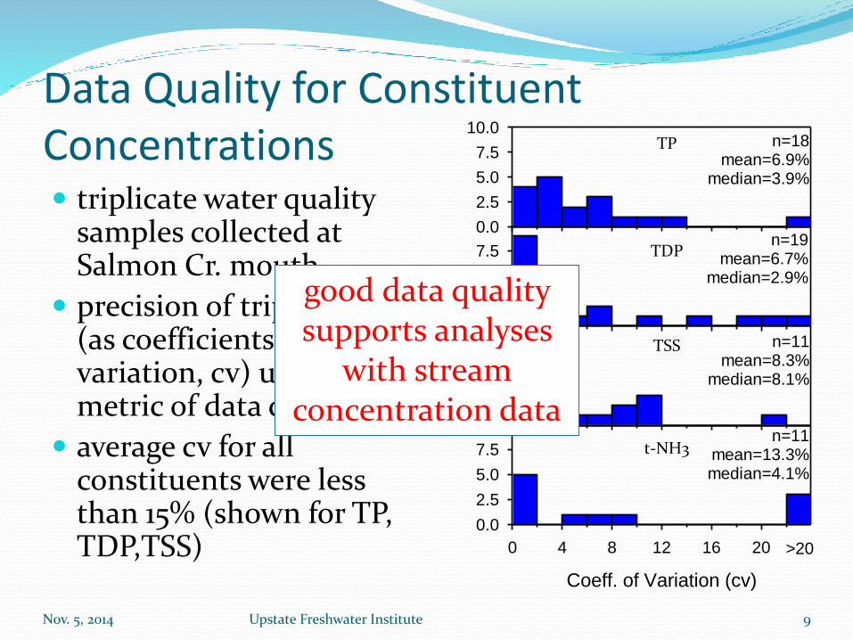
Data Quality for Constituent Concentrations triplicate water quality
samples collected at Salmon Cr. mouth
precision of triplicates (as coefficients of variation, cv) used as a metric of data quality
average cv for all constituents were less than 15% (shown for TP, TDP,TSS)
Nov. 5, 2014 Upstate Freshwater Institute 9
Coeff. of Variation (cv)
0 4 8 12 16 20
0.0
2.5
5.0
7.5
>20
0.0
2.5
5.0
7.5
10.0
Count
0.0
2.5
5.0
7.5
0.0
2.5
5.0
7.5
n=11mean=13.3%median=4.1%
n=18mean=6.9%
median=3.9%
n=19mean=6.7%
median=2.9%
n=11mean=8.3%
median=8.1%
TP
TDP
TSS
t-NH3
good data quality supports analyses
with stream concentration data

Constituent Concentrations: Fall Creek Time Series for TP, PP
TP dominated by PP
PP increased dramatically during periods of high flow (see three largest events monitored : June 30, July 21, and August 8-9)
peak TP and PP concentrations were 996 and 927 µg/L, respectively
Nov. 5, 2014 Upstate Freshwater Institute 10
M A M J J A S O N
P(µ
g/L
)
0
250
500
750 TP
PP
Flo
w
(m3/s
)
0
25
50
75
100
2013

Fall Creek During High Flow
Nov. 5, 2014 Upstate Freshwater Institute 11

Constituent Concentrations: Fall Creek Time Series for Dissolved P
Nov. 5, 2014 Upstate Freshwater Institute 12
SRP, SUP demonstrated some seasonality
SRP, SUP were generally lowest during periods of low flow and increased during runoff events
increases observed were less substantial than for particulate constituents
M A M J J A S O N
P(µ
g/L
)
0
25
50
75 TDP
SRP
SUP
Flo
w
(m3/s
)
0
25
50
75
100
2013
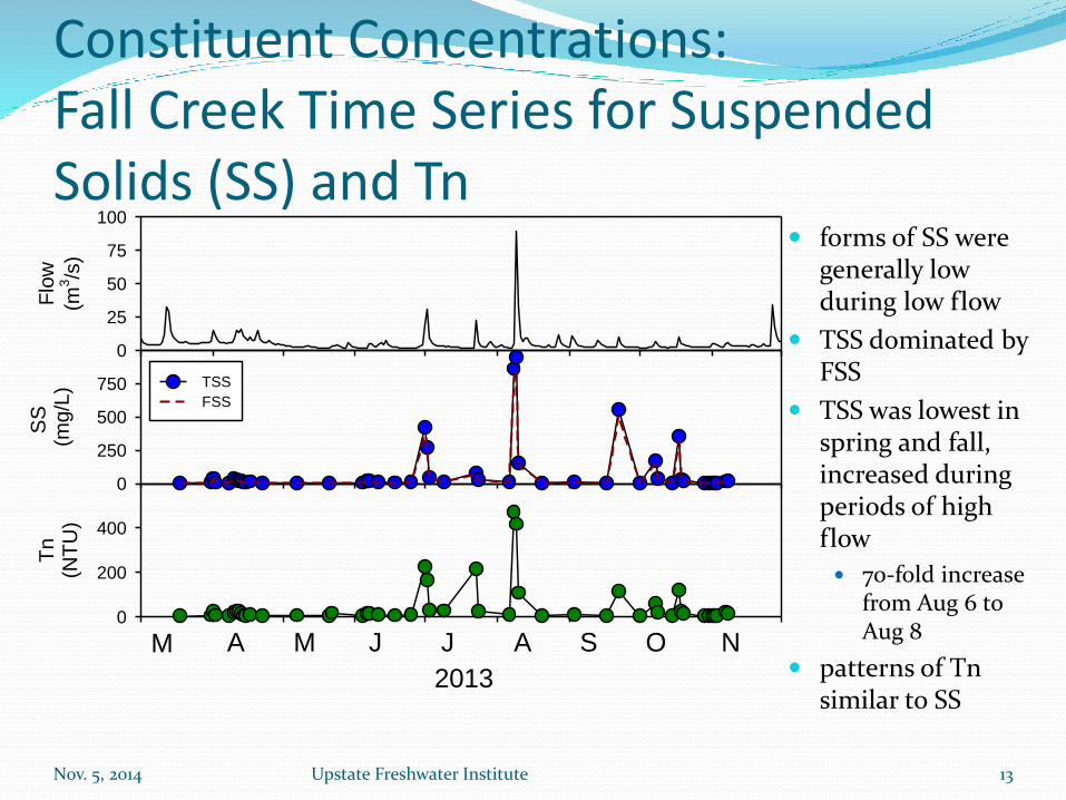
Constituent Concentrations:Fall Creek Time Series for Suspended Solids (SS) and Tn
forms of SS were generally low during low flow
TSS dominated by FSS
TSS was lowest in spring and fall, increased during periods of high flow
70-fold increase from Aug 6 to Aug 8
patterns of Tn similar to SS
Nov. 5, 2014 Upstate Freshwater Institute 13
M A M J J A S O N
Tn
(NT
U)
0
200
400
SS
(m
g/L
)
0
250
500
750 TSS
FSS
Flo
w
(m3/s
)
0
25
50
75
100
2013

Constituent Concentrations: Time Series for Fall Creek
other dissolved constituents (DOC, t-NH3, Si) similar to dissolved P
generally lowest during periods of low flow and increased during runoff events
increases during high flow, less substantial than for particulates
NOX highest in spring and fall
dominant form of dissolved N
Nov. 5, 2014 Upstate Freshwater Institute 14
M A M J J A S O N
DO
C(m
g/L
)
0
4
8
t-N
H3
(µg/L
)
0
50
100
150
NO
X
(µg/L
)
0
2500
5000
7500
Si
(mg/L
)
0
2
4
6
Flo
w
(m3/s
)
0
25
50
75
100
2013

Constituent Concentrations: Example Box-Whiskers for Low Flow vs. High Flow for Fall Creek
large increases in mean concentration between low and high flow for particulates
dissolved constituents showed increases from low-to-high flow but less substantial than for particulates
Fall Creek patterns (not necessarily magnitudes) were similarly demonstrated in other streams
Nov. 5, 2014 Upstate Freshwater Institute 15
LOW HIGHP
P (
µg
/L)
0
100
200
300
400
500
LOW HIGH
SR
P (
µg
/L)
0
10
20
30
40
LOW HIGH
SU
P (
µg
/L)
0
10
20
30
40
LOW HIGH
Tn
(N
TU
)
0
50
100
150
200
250
300
LOW HIGH
TS
S (
mg
/L)
0
100
200
300
400
500
LOW HIGH
t-N
H3 (
µg
/L)
0
20
40
60
80
100
LOW HIGH
NO
X (
µg
/L)
0
1000
2000
3000
4000
LOW HIGH
DO
C (
mg
/L)
0
5
10
15
LOW = 25.9HIGH = 109.6
LOW = 6.4HIGH = 9.8
LOW = 7.2HIGH = 8.6
LOW = 10.2HIGH = 72.4
LOW = 10.4HIGH = 141.6
LOW = 23.4HIGH = 26.6
LOW = 1,237HIGH = 2,205
LOW = 5.2HIGH = 6.3
median
mean
75th
percentile
25th
percentile
Key:
90th
percentile
95th
percentile
10th
percentile
5th
percentile

Constituent Concentrations: Comparisons Between Tributaries
Nov. 5, 2014 Upstate Freshwater Institute 16
TP
(µg/L
)
0
20
40
60
PP
(µg/L
)
0
20
40
FC CI SC TC 6M
SR
P(µ
g/L
)
0
10
20
0
100
200
300
400
0
100
200
300
FC CI SC TC 6M
0
10
20
At low flow:
TP, PP highest average in Fall Creek
Tn, SS similar to PP
SRP highest for Salmon Creek
Low Flow High Flow
At high flow:
TP, PP highest average in Cayuga In. Creek
SRP highest for Salmon Creek

Constituent Concentrations: Comparisons Between Tributaries
Nov. 5, 2014 Upstate Freshwater Institute 17
Low Flow High Flow
At high flow:
high flow conditions similar to low flow conditions
NOX >> t-NH3
DO
C(m
g/L
)
0
2
4
6
8
t-N
H3
(µg/L
)
0
20
40
FC CI SC TC 6M
NO
X
(µg/L
)
0
2000
4000
6000
0
2
4
6
8
0
20
40
FC CI SC TC 6M
0
2000
4000
6000
At low flow:
DOC highest in Fall Cr. and Salmon Cr.
t-NH3 similar for all streams
NOX highest for Salmon Creek

Constituent Concentrations:Phosphorus Ratios TP
dominated by PP for Fall, Cayuga In. Cr., Six Mile Cr., and Taugh Cr. at low and high flow
at low flow Salmon Cr. had the lowest PP:TP ratio (i.e., Salmon Cr. TP dominated by TDP)
PP:TP ratio increased with increasing flow for all tribs
TDP dominated by SUP for Fall Cr. and
Cayuga In. Cr. dominated by SRP for Salmon Cr.
and Six Mile Cr. bioavailability implications SRP:TDP increased slightly with
increasing flow (all but Six Mile Cr.)
Nov. 5, 2014 Upstate Freshwater Institute 18

Outline1. Goals and Analysis Components
2. Monitoring
3. Constituent Concentrations
4. Concentration-Driver Relationships
5. Load Estimation Techniques and Best Methods
6. 2013 April – October Load Estimates
7. P bioavailability and Loads
8. 2000-2012, Loading and Magnitudes of Interannual Variability
9. Inlet Channel Effects: Case for Inlet Load Adjustments
10. Summary
Nov. 5, 2014 Upstate Freshwater Institute 19

Concentration-Driver Relationships: Concentration-Flow
conc.-Q relationships were stronger for particulates than for dissolved constituents
significance, strength of fit varied between parameters, streams
Nov. 5, 2014 Upstate Freshwater Institute 20
Q (m3/s)
0.1 1 10 100 1000
PP
(µ
g/L
)
1
10
100
1000
Q (m3/s)
0.1 1 10 100 1000
SR
P (
µg/L
)
0.1
1
10
100
Q (m3/s)
0.1 1 10 100 1000
NO
X (
µg/L
)
100
1000
10000
PP=8.20·Q0.768
r2=0.39
p<0.001
SRP=2.64·Q0.251
r2=0.04
p=0.19
NOx=1023·Q0.01
r2=0.00
p=0.96
TSS=2.03·Q1.194
r2=0.50
p<0.001
Q (m3/s)
0.1 1 10 100 1000
TS
S (
mg/L
)
0.1
1
10
100
1000
Fall Creek

Q (m3/s)
1 10 1 10 1 10 1001 10
PA
Vm
(1/m
)
0.01
0.1
1
10
100
Concentration-Driver Relationships: Flow-Projected Area Minerogenic Particles per Unit Volume (PAVm)
valuable metric for P and optical impacts of inorganic (mineral) particles
4 size classes support modeling of fate of minerogenic particle inputs to lake
Nov. 5, 2014 Upstate Freshwater Institute 21
Class 1 Class 2 Class 3 Class 4
positive dependency on Q
Fall Creek
0.1 1 10 30
0
10
20
30
40
Particle size (m)
Cu
mu
lati
ve P
AV
m (
cm2 /L
)
Size-class-2 PAVm
Size-class-3 PAVm
4 size classes:Class 1: 2 mClass 2: 25.6 mClass 3: 5.611 mClass 4: 11 m

Concentration-Driver Relationships: Concentration-Air Temperature
conc.-air T relationships not significant for particulates exception Fall Cr.
conc.-air T significance, strength of fit better for dissolved constituents than for particulates better predictor
than flow for most parameters, streams
Nov. 5, 2014 Upstate Freshwater Institute 22
Fall Creek
Air T (°F)
20 30 40 50 607080
PP
(µ
g/L
)
1
10
100
1000
Air T (°F)
20 30 40 50 607080
SR
P (
µg/L
)
0.1
1
10
100
Air T (°F)
20 30 40 50 607080
NO
X (
µg/L
)
100
1000
10000
PP=0.07·T1.536
r2=0.12
p=0.02
SRP=0.002·Q2.450
r2=0.33
p<0.001
NOx=57.5E4·Q
1.596
r2=0.24
p=0.001
TSS=0.02·Q1.711
r2=0.09
p=0.04
Air T (°F)
20 30 40 50 607080
TS
S (
mg/L
)
0.1
1
10
100
1000

Concentration-Driver Relationships: Concentration-Turbidity
exploratory
conc.-Tn relationships very strong for particulates r2>0.8
p<0.001
conc.-Tn results varied between parameters, streams for dissolved constituents good predictor for
some parameters, streams
Nov. 5, 2014 Upstate Freshwater Institute 23
Fall Creek
Tn (NTU)
1 10 100 1000
PP
(µ
g/L
)
1
10
100
1000
Tn (NTU)
1 10 100 1000
SR
P (
µg/L
)
0.1
1
10
100
Tn (NTU)
1 10 100 1000
NO
X (
µg/L
)
100
1000
10000
PP=3.13·Q0.852
r2=0.93
p<0.001
SRP=1.28·Q0.409
r2=0.22
p<0.001
NOx=1538·Q-0.127
r2=0.04
p=0.24
TSS=0.73·Q1.168
r2=0.92
p<0.001
Tn (NTU)
1 10 100 1000
TS
S (
mg/L
)
0.1
1
10
100
1000

Outline1. Goals and Analysis Components
2. Monitoring
3. Constituent Concentrations
4. Concentration-Driver Relationships
5. Load Estimation Techniques and Best Methods
6. 2013 April – October Load Estimates
7. P bioavailability and Loads
8. 2000-2012, Loading and Magnitudes of Interannual Variability
9. Inlet Channel Effects: Case for Inlet Load Adjustments
10. Summary
Nov. 5, 2014 Upstate Freshwater Institute 24

Load Estimation Techniques Adopted FLUX32 (F32) Load Estimation Software
Regression Methods 5 methods
Non-regression methods 3 methods
Manual Methods Multiple linear regression with flow, air T
C/Q regression using instantaneous flow (Fall Cr. only)
C/Q regression using instantaneous flow with event load estimates (Fall Cr. only)
Monthly mean method
Nov. 5, 2014 Upstate Freshwater Institute 25

Load Estimation Results for Fall Creek:All Methods, April-October
Nov. 5, 2014 Upstate Freshwater Institute 26
Method PP Load (kg) SUP Load (kg) SRP Load (kg)
F32 method 6 C/Q interpolated 8,010 742 855
F32 method 6 C/Q 11,289 770 1,202
F32 method 5 C/Q adj. 8,156 755 893
F32 method 4 C/Q flow wtd. adj. 8,300 759 907
F32 Rising/Falling limb 8,008 739 850
Manual regr. 10,251 746 1,108
Manual regr. with events 10,223 645 1,153
Multiple Linear Regression 8,896 784 971
F32 method 3 Beale’s Ratio Estimator 10,778 802 1,095
F32 method 2 flow weighted conc. 10,223 794 1,055
F32 method 1 average load 12,425 964 1,298
Monthly mean 12,259 828 1,085
---regression methods (range) 8,008-11,289 739-770 850-1,202
---non-regression methods (range) 10,223-12,259 794-828 1,055-1,095

Load Estimation Results for Fall Creek Using Different Methods, April-October
Nov. 5, 2014 Upstate Freshwater Institute 27
PP
L (
mt)
0
5
10
15
20
25
SU
PL (
mt)
0.0
0.5
1.0
1.5
F3
2 M
6 R
eg
r.,
Inte
rp.
F3
2 M
6 R
eg
r.
F3
2 M
5 R
eg
r.
F3
2 M
4 R
eg
r.
F3
2 H
yd
ro S
ep
Ma
nu
al R
eg
r.
Ma
nu
al R
eg
r.,
Eve
nts
Ma
nu
al M
LR
F3
2 M
3
F3
2 M
2
F3
2 M
1
Mo
nth
ly M
ean
SR
PL (
mt)
0.0
0.5
1.0
1.5
2.0
Avg. All
Methods
w/ 95% CI
BestEstimate
Avg.
Regr.
Methods
w/ 95% CI
PPL
okay agreement, regression methods within 10-22% of best method
SUPL
strong agreement, regression methods within 1-6% of best methods
SRPL
okay agreement, regression methods within 7-20% of best method
this level of uncertainty is not
uncommonin load estimation

Best Methods for Load Estimation Particulate Constituents
FLUX32 C/Q Regression, Interpolation daily time step significant relationships between concentration and flow stratified by flow regime supported by differences in C/Q slopes between low and
high flow allows smooth interpolation between observations using defined C/Q
relationship estimates air T generally not significantly related to particulate concentration usually less uncertainty than non-regression methods
Dissolved Constituents Multiple Linear Regression with Q, air T as drivers
daily time step flow generally not strong, rarely significant predictor of concentration concentration-air T significant in most cases multiple regression model better than C/Q alone
Nov. 5, 2014 Upstate Freshwater Institute 28

Best Methods for Load Estimation:Unmonitored Tributaries
Monitored Watershed 5 largest tribs, ~60% of watershed area assumed 60% of hydrologic inflow FC, CI, SC, TC, 6M (yellow)
Unmonitored Watershed 40 % of lake’s watershed many small streams (each < 3.5% of
lake’s watershed) assumed unmonitored area ∝ to
unmonitored inflow
Unmonitored Load Estimates prorated monitored loads to whole-lake
watershed loads based on ratio of monitored:unmonitored watershed areas
consistent with land use information
Nov. 5, 2014 Upstate Freshwater Institute 29
SC
FC
6MCI
TC
~40% unmonitored

Outline1. Goals and Analysis Components
2. Monitoring
3. Constituent Concentrations
4. Concentration-Driver Relationships
5. Load Estimation Techniques and Best Methods6. 2013 April – October Load Estimates
7. P bioavailability and Loads
8. 2000-2012, Loading and Magnitudes of Interannual Variability
9. Inlet Channel Effects: Case for Inlet Load Adjustments
10. Summary
Nov. 5, 2014 Upstate Freshwater Institute 30

2013 April-October Loading Estimates:Primary Constituents
Nov. 5, 2014 Upstate Freshwater Institute 31
Tributary
TP
(kg)
PP
(kg)
TDP
(kg)
SRP
(kg)
SUP
(kg)
Tn
(NTU·m3)
Fall Creek 9,765 8,010 1,755 971 784 5.86E+09
Cayuga Inlet Creek 9,564 9,208 356 167 189 1.04E+10
Salmon Creek 5,792 4,171 1,621 1,234 387 3.02E+09
Taugh. Creek 4,931 3,639 1,291 813 479 4.96E+09
Six Mile Creek 2,500 2,036 464 321 143 2.77E+09
Unmonitored 22,157 18,422 3,735 2,387 1,349 1.84E+10
Point Sources 1,415 745 669 302 368 -
Total Watershed 56,124 46,232 9,892 6,194 3,698 4.54E+10
sum of daily estimates

2013 April-October Loading Estimates:Secondary Constituents
Nov. 5, 2014 Upstate Freshwater Institute 32
Tributary
TSS
(kg)
FSS
(kg)
VSS
(kg)
t-NH3
(kg)
NOX
(kg)
DOC
(kg)
Si
(kg)
Fall Creek 11,196,214 10,040,965 1,155,249 2,755 110,606 551,300 343,068
Cayuga Inlet Creek 10,429,918 9,640,675 789,243 889 15,656 154,949 230,061
Salmon Creek 2,866,144 2,493,251 372,893 1,179 225,205 266,865 231,276
Taugh. Creek 3,227,723 3,003,859 223,864 1,514 65,289 264,981 343,492
Six Mile Creek 2,738,443 2,456,535 281,908 584 6,663 109,585 125,778
Unmonitored 20,731,759 18,810,156 1,921,602 4,711 288,203 917,309 866,936
Point Sources - - - - - - -
Total Watershed 51,190,201 46,445,441 4,744,760 11,631 711,621 2,264,989 2,140,611
sum of daily estimates

Non-point Source
Point Source
2013 April-October Loading Estimates: Phosphorus
TPL dominated by PPL
Fall Cr. and Cayuga In. – largest individual contributors of PPL
Fall Cr. – 8.0 mt (17.3%) Cayuga In. – 9.2 mt (20%)
Fall Cr. and Salmon Cr. – largest contributors of TDPL
Fall Cr. – 1.8 mt (17.7%) Salmon Cr. – 1.6 mt (16.4%)
Cayuga Lake PPL and TDPL is dominated by non-point sources
Nov. 5, 2014 Upstate Freshwater Institute 33
PPL
93%
TDPL
7%1.6%
98.4%
FC CI SC TC 6M UM PTS
P (
mt)
0
5
10
15
20
25
PP
SUP
SRP

2013 April-October Loading Estimates: Turbidity and Forms of SS
TSSL dominated by FSSL (minerogenic particles) 87-93%
Fall Cr. and Cayuga Inlet Cr. – largest individual sources
TnL patterns were similar to TSSL
Nov. 5, 2014 Upstate Freshwater Institute 34
FC CI SC TC 6M UM
SS
(10
3 m
t)
0
5
10
15
20
25
FSS
VSS
FC CI SC TC 6M UM
Tn (
10
6 N
TU
m3)
0.0
5.0e+3
1.0e+4
1.5e+4
2.0e+4
2.5e+4

2013 April-October Loading Estimates: PAVm
apportioned according to 4 size classes
size class 2 contributes the most (34%)
smallest size class (PAV1) contributes the least
general similarity to SS and Tn patterns
Nov. 5, 2014 Upstate Freshwater Institute 35
FC CI SC 6M UnMon.
PA
Vm
Load
(10
6·m
2)
0
2000
4000
6000
PAV1
PAV2
PAV3
PAV4
Total PAVm Load (m2)
PA
Vm
Load
(10
6·m
2)
0
5000
10000
15000
10%34%
30%
26%

2013 April-October Loading Estimates: NOX
Salmon and Fall Cr. largest individual sources
NOXL >> than t-NH3L
Nov. 5, 2014 Upstate Freshwater Institute 36
FC CI SC TC 6M UM
t-N
H3 (
mt)
0
1
2
3
4
5
6
FC CI SC TC 6M UMN
OX (
mt)
0
100
200
300
400

TD
P (
mt)
0
1
2
3
4
DO
C (
mt)
0
250
500
750
FC CI SC TC 6M UMN
OX (
mt)
0
100
200
300
PP
(m
t)
0
5
10
15
20
High flow load
Low flow load
FC CI SC TC 6M UM
Tn
(10
6 N
TU
·m3)
0.0
5.0e+3
1.0e+4
1.5e+4
TS
S
(10
3 m
t)
0
5
10
15
20
2013 April-October Loading Estimates:Low vs High Flow
delivered during high flow 18% of days for Fall Cr. during study
91% of PPL and TnL
97% of TSSL
other particulates similar
delivered during high flow 70% of TDPL
61 % of DOCL
65 % of NOXL
Nov. 5, 2014 Upstate Freshwater Institute 37
Particulates Dissolved
PP
(m
t)
0
5
10
15
20
High flow load
Low flow load
FC CI SC TC 6M UM
Tn
(10
6 N
TU
·m3)
0.0
5.0e+3
1.0e+4
1.5e+4
TS
S
(10
3 m
t)
0
5
10
15
20
majority of constituent loads delivered during
high flow

2013 April-October Loading Estimates:As Yields (kg/km2)
yield = load ÷ watershed area
to indicate potency of individual sources
TP yield was dominated by PP
Cayuga Inlet had the largest TP yield 40 kg/km2
TDP yield was dominated by SRP Taugh Cr. and Salmon Cr.
~ 7 kg/km2
Nov. 5, 2014 Upstate Freshwater Institute 38
TP
(kg/k
m2)
0
10
20
30
40
50
PP
TDP
FC CI SC TC 6M UM
TD
P
(kg/k
m2)
0
2
4
6
8 SUP
SRP

2013 April-October Loading Estimates:As Yields (kg/km2)
Nov. 5, 2014 Upstate Freshwater Institute 39
TSS yield was dominated by FSS
Cayuga Inlet had the largest TSS yield 43.3·103 kg/km2
Fall Cr. was second highest for TSS yield 33.8·103 kg/km2
Tn similar to TSS patterns Taugh. Cr. and Six Mile
Creek ranked 2nd and third
20.4 and 18.7 kg/km2FC CI SC TC 6M UM
Tn
(10
6 N
TU
·m3/k
m2)
0
10
20
30
40
TS
S
(10
3 k
g/k
m2)
0
10
20
30
40
50
FSS
VSS

Outline1. Goals and Analysis Components
2. Monitoring
3. Constituent Concentrations
4. Concentration-Driver Relationships
5. Load Estimation Techniques and Best Methods
6. 2013 April – October Load Estimates7. P bioavailability and Loads
8. 2000-2012, Loading and Magnitudes of Interannual Variability
9. Inlet Channel Effects: Case for Inlet Load Adjustments
10. Summary
Nov. 5, 2014 Upstate Freshwater Institute 40

Phosphorus Bioavailability
Tributarymean
PPfBAP (%)
CVmeanSUP
fBAP (%)CV
Fall Cr. 10.6 60 92.7 7
Cayuga Inlet Cr. 5.7 64 59.7 24
Salmon Cr. 19.2 70 84.4 20
Six Mile Cr. 6.0 69 65.5 49
CHWWTP 25.4 11 62.7 16
IAWWTP 1.2 83 73.2 29
LSC - - 8.2 141
fBAP found to be watershed specific, correlated to % watershed in agriculture
%Ag-PP fBAP, r =0.97
%Ag-SUP fBAP, r = 0.78
Nov. 5, 2014 Upstate Freshwater Institute 41
fBAP – fraction of P bioavailable
PP was least bioavailable
SUP was mostly bioavailable
SRP (not shown) was nearly completely available (> 93%)
Percent Land Use in Ag. (%)
0 25 50 75
fB
AP
(%
)
0
25
50
75
100
SC
SC
FC
FC
CI
CI6M
6M
PP
SUP

2013 Tributary Loading Estimates: Bioavailable P, April – October
May 19, 2014 Upstate Freshwater Institute 42
TPL
(56.1 mt)
FCSC
6M
TC
CI
Unmon.
Total LoadsP Fractions
~ 73% reduction
BAPL
(14.9 mt)
Bioavailable LoadsP Fractions

Apportionment of BAP Loads, 2013
May 19, 2014 Upstate Freshwater Institute 43
Percent Contribution (%)
Source BAPL
Fall Cr. 16.9
Cayuga In. 5.3
Salmon Cr. 15.8
Six Mile Cr. 3.5
Taugh. Cr. 10.7
Unmon. Tribs. 43.4
summed (%) 95.7
IAWWTP 1.4
CHWWTP 0.5
minor WWTP 0.9
LSC 1.5
summed (%) 4.3
summed (%) 100
non-pointsources
pointsources

Outline1. Goals and Analysis Components
2. Monitoring
3. Constituent Concentrations
4. Concentration-Driver Relationships
5. Load Estimation Techniques and Best Methods
6. 2013 April – October Load Estimates
7. P bioavailability and Loads8. 2000-2012, Loading and Magnitudes of Interannual
Variability
9. Inlet Channel Effects: Case for Inlet Load Adjustments
10. Summary
Nov. 5, 2014 Upstate Freshwater Institute 44

BA
PL (
mt)
0
10
20
30
40
50
2000-201212y
no 201113y tribs SC PtS
2013
14.9
2.34 0.65
29.625.1
Load Estimates for the 2002-2012 Period: Magnitudes and Interannual Variability 2013 conc.-driver relationships applied
comparison to 2013 estimates
total, Salmon Cr., summed point sources
May 19, 2014 Upstate Freshwater Institute 45
• 2013 close to long-term mean
• interannual variability large (± 1 std. dev.)
• >> Salmon Cr.
• >> summed point sources
• important for reasonable expectations for management actions
interannualvariability

Outline1. Goals and Analysis Components
2. Monitoring
3. Constituent Concentrations
4. Concentration-Driver Relationships
5. Load Estimation Techniques and Best Methods
6. 2013 April – October Load Estimates
7. P bioavailability and Loads
8. 2000-2012, Loading and Magnitudes of Interannual Variability
9. Inlet Channel Effects: Case for Inlet Load Adjustments
10. Summary
Nov. 5, 2014 Upstate Freshwater Institute 46

Adjustments in P/Suspended Solids Loading from Effects of Inlet Channel Necessary
strong evidence that the P and SS loads delivered to the lake from the inlet channel are lower than the sum of tributary inputs (2013 example) in-channel deposition
instrument deployments together with conc-Tn relationships will be used to estimate the effective loading (subsequently)
development of adjusted loads is necessary to support realistic predictions for the shelf
Nov. 5, 2014 Upstate Freshwater Institute 47
Tn (
NT
U)
1
10
100
1000
10000
Q (
cfs
)
0
1000
2000
3000
4000Cay. Inlet
6 Mile Crk.
2013
05/01 07/01 09/01 11/01
TS
S (
mg/L
)
1
10
100
1000
10000
large differences
large differences
IL
Cayuga In. Cr.
6Mile
Fall Cr.

Estimation of Constituent Concentration Using In Situ Deployments
Nov. 5, 2014 Upstate Freshwater Institute 48
TD
P (
µg/L
)1
10
100
PP
(µ
g/L
)
1
10
100
1000
In Situ Tn (NTU)
1 10 100 1000
SR
P (
µg/L
)
0.1
1
10
100
In Situ Tn (NTU)
1 10 100 1000
TS
S (
mg/L
)
1
10
100
1000[PP] =9.29·Tn
0.517
r ²=0.71
[TDP] =5.25·Tn0.366
r ²=0.67
[SRP] =1.21·Tn0.583
r ²=0.60
[TSS] =1.93·Tn0.801
r ²=0.84
Instrument deployments
Frequent (>> daily) Tn (driver)measurements
M J J A S O
In S
itu
Tn (
NT
U)
1
10
100
1000
Concentration-driver (Tn) relationships
frequent estimates of concentrations and daily
flows used to estimate daily loads
advantage in load estimation
and certainty

Outline1. Goals and Analysis Components
2. Monitoring
3. Constituent Concentrations
4. Concentration-Driver Relationships
5. Load Estimation Techniques and Best Methods
6. 2013 April – October Load Estimates
7. P bioavailability and Loads
8. 2000-2012, Loading and Magnitudes of Interannual Variability
9. Inlet Channel Effects: Case for Inlet Load Adjustments10. Summary
Nov. 5, 2014 Upstate Freshwater Institute 49

Summary comprehensive event-based
monitoring of major tributaries conducted in 2013
constituent concentrations increased during high flow, particularly metrics of particulates
concentration-driver relationships developed to estimate conditions on non-monitored days Q and T, relationships of varied
strengths
loading estimates made (daily time step) to support modeling for multiple constituents multiple protocols, reasonable closure majority of loads delivered during high
flow intervals sediment loads mostly inorganic apportioned according sources
Nov. 5, 2014 Upstate Freshwater Institute 50

Summary adjustments of constituent loading
from tributaries entering the Inlet Channel are required because of depositional losses
bioavailability of P forms and development of BAPL’s PP – limited, SUP – mostly, SRP ~
completely
BAPL ~ 25% of TPL for the lake
point source contributions are minor (< 5%)
interannual variations (driven by Q) are large relative to individual source contributions
Nov. 5, 2014 Upstate Freshwater Institute 51

Questions
Nov. 5, 2014 Upstate Freshwater Institute 52