2012 course syllabus vibration fatigue · vibration fatigue dr nwm bishop dynamics • •what is a...
TRANSCRIPT

1
RLD Ltd ©
2012
Dr NWM Bishop 290
Course Syllabus Vibration Fatigue
Dr NWM Bishop
Dynamics
• What Is A PSD • Time v Frequency Domain • Transfer Functions • Structural Analysis Using PSD’s • RMS Levels and Hand Calculations • Practical PSD Calculations • Probability & Statistical Concepts
Fatigue & Dynamics
• PSD Statistics • Hand Calculations in Time & Freq Domains • Methods For Test Acceleration • RCC From PSD’s • Fatigue Damage Editing
RLD Ltd 291 ©
2012
What is a PSD

2
RLD Ltd ©
2012
Dr NWM Bishop 292
Key elements of a PSD type analysis
What is a PSD
How to build a PSD input from specified details
How to do structural analysis using PSD’s
How to calculate RCC’s and fatigue life from the
response PSD’s
RLD Ltd ©
2011
Dr NWM Bishop 293
Features�
– Multi input loads�
– Correlation effects using Cross PSD’s�
– Resolution of stresses onto Principal planes�
– Calculation of response PSD using TF’s and input PSD’s�
– Calculate fatigue life from PSDs�
Vibration Fatigue in the Frequency DomainTransfer Functions on
component axes�
Transfer Functions rotated on to Principal planes by MSC
Fatigue�
� Response PSD’s calculated by MSC Fatigue�
0
500
1000
1500
2000
2500
3000
3500
0 20 40 60 80 100 120 140 160 180 200
4%
5%
6%
8%
0.00
0.01
0.02
0.03
0.04
0.05
0.06
0 100 200
A
B
020406080100120140160
0 20 40 60 80 100 120 140 160 180 200
0
500
1000
1500
2000
2500
3000
3500
0 20 40 60 80 100 120 140 160 180 200
4%
5%
6%
8%
0.00
0.01
0.02
0.03
0.04
0.05
0.06
0 100 200
A
B
020406080100120140160
0 20 40 60 80 100 120 140 160 180 200
Input PSD [A]�
Transfer Function [B]�
Response PSD [C]�
Rainflow histogram and fatigue life calculated by
MSC Fatigue�
293

3
RLD Ltd ©
2012
Dr NWM Bishop 294
Random v Deterministic
RLD Ltd ©
2012
Dr NWM Bishop 295
Alternative descriptions for response environments
RandomDISPLAY OF SIGNAL: Y27A.PSD
Deterministic

4
RLD Ltd ©
2012
Dr NWM Bishop 296
Fourier Series Deterministic (time)
Random(time)
=
404040
444
333
222
111
,,.
,,.
,,,,,,,,
φ
φ
φ
φ
φ
φ
fa
fa
fafafafa
iii
RLD Ltd ©
2012
Dr NWM Bishop 297
Fourier Transforms (retaining phase) Deterministic (frequency)
Random(time)
=
404040
444
333
222
111
,,.
,,.
,,,,,,,,
φ
φ
φ
φ
φ
φ
fa
fa
fafafafa
iii
amplitudes phases
This curve is actually a histogram

5
RLD Ltd ©
2012
Dr NWM Bishop 298
PSD’s (discarding phase) Random
(frequency)
Random(time)
=
4040
44
33
22
11
,.,.,,,,
fa
fa
fafafafa
ii
Amplitudes - squared
Curve is now continuous
RLD Ltd ©
2012
Dr NWM Bishop 299
Fourier Transforms – recreating time signals Random
(frequency)
Random(time)
=
4040
44
33
22
11
,.,.,,,,
fa
fa
fafafafa
ii
Plus phases
π2
π21
)(φp
404321 ,,,,,,,,, φφφφφφ i

6
RLD Ltd ©
2012
Dr NWM Bishop 300
Equivalence in the time and frequency domains
Is the regenerated time signal exactly equivalent to the original time history?
No!
Does it matter?
No!
Why?
RLD Ltd ©
2012
Dr NWM Bishop 301
Equivalence in the time and frequency domains
Consider the original time history again
300 seconds
When considering the original time history was the 300 second segment of time signal before, or after, the one measured, equivalent?
No!
Does it matter?
No, as long as the sample was long enough so that the statistics of it were the same. For example, the mean, stress range values, peak rate etc.

7
RLD Ltd ©
2012
Dr NWM Bishop 302
Conclusion
In order to calculate fatigue damage we can work in whatever domain is most sensible in terms of ease, and accuracy, of structural analysis.
RLD Ltd 303 ©
2012
Time v Frequency Domain
8
RLD Ltd ©
2012
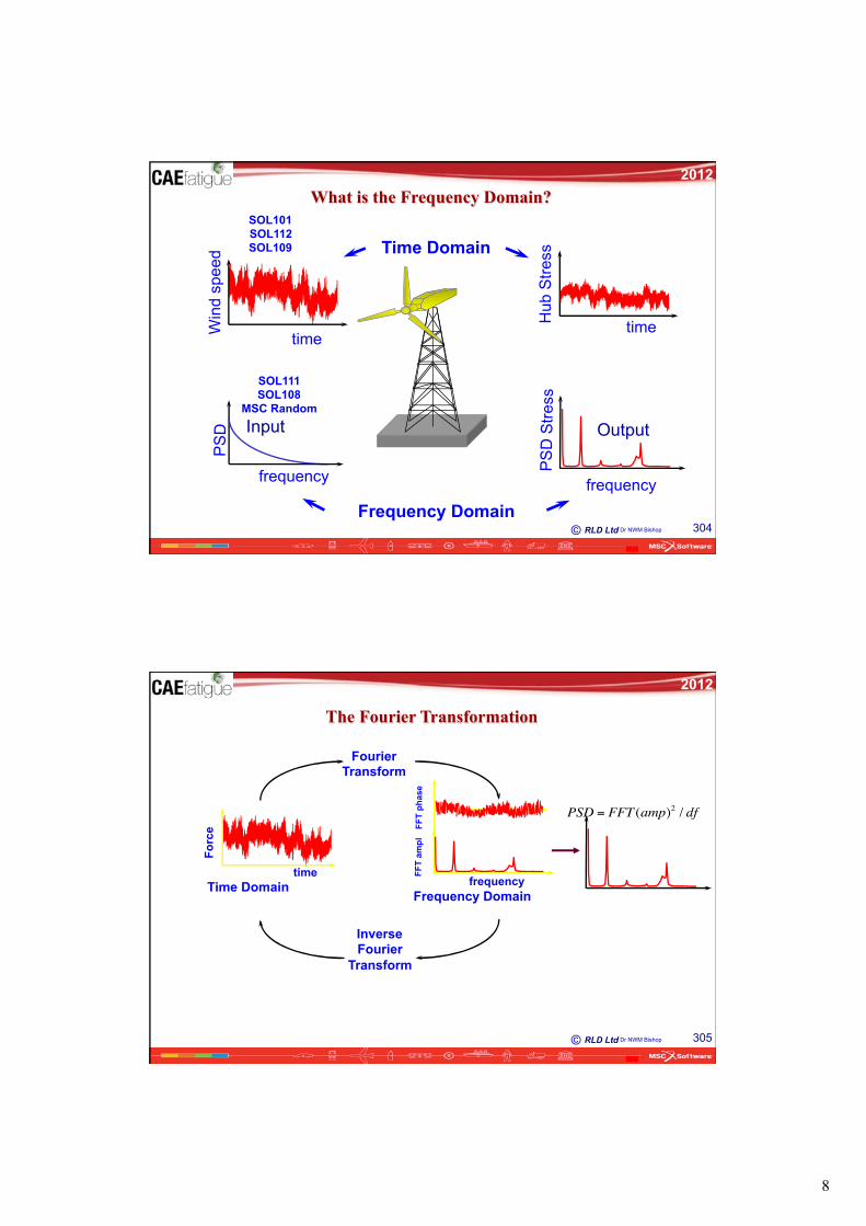
Dr NWM Bishop 304
What is the Frequency Domain?
frequency
time Win
d sp
eed
Frequency Domain
Time Domain
PS
D S
tress
Output
PS
D
frequency
Input
time Hub
Stre
ss
SOL101 SOL112 SOL109
SOL111 SOL108
MSC Random
RLD Ltd ©
2012
Dr NWM Bishop 305
The Fourier Transformation
FourierTransform
InverseFourier
Transform
time
Forc
e
Time Domain
FFT
ampl
frequency Frequency Domain
PSD = FFT (amp)2 / df
FFT
phas
e

9
RLD Ltd 306 ©
2012
Transfer Functions
RLD Ltd ©
2012
Dr NWM Bishop 307
What is the Transfer Function?
time Win
d sp
eed
Frequency Domain
Time Domain
PS
D S
tress
frequency
Output
PS
D
frequency
Input
time Hub
Stre
ss
Transfer function
10
RLD Ltd ©
2012
Dr NWM Bishop 308
Mass M
Stiffnes K
Sinusoidal Displacement with amplitude X
Damping C
time
A
The FE Analysis Environment What is a Transfer Function ?
Sinusoidal force with amplitude Fand frequency ω�
T
1.0
4.0
2 4 6 8 10 12 14 16 18 20 220
ω�frequency
Transfer function
The amplitude of the displacement X is found by:
FTX ⋅=
Sinusoidal Force
RLD Ltd ©
2012
Dr NWM Bishop 309
PSD Approach
H(f) = Complex frequency transfer function for each load case Sab(f) = Auto & Cross-Power Spectra
)(.)(.)()(2
1
2
1fSfHfHfS abba
ba∑∑==
=
Transfer Function [B]
Output PSD [C]
Input PSD [A]
A x B = C
Mass M
Stiffness K
Sinusoidal Stress with amplitude
Damping C
Sinusoidal Force
What are the units?

11
RLD Ltd ©
2012
Dr NWM Bishop 310
Different parts of the Transfer Function ?
frequency
Transfer function
Dam
ping controlled
Mass controlled
Stiffness controlled
RLD Ltd 311 ©
2012
Structural Analysis Using PSD’s

12
RLD Ltd ©
2012
Dr NWM Bishop 312
Transfer Function [B]
A x B = C
4 6
5
1 2 3
The process of calculating a transfer function
Output PSD [C]
1
2
3 4 6
5
Input PSD [A]
1
2
3
654
RLD Ltd ©
2012
Dr NWM Bishop 313
Example: How Transfer Functions Work Consider the following base acceleration input PSD
0.0010
0.0100
0.1000
10 100 1000Frequency (Hz)
PSD
am
plitu
de (g
^2/H
z)
0.00
0.01
0.02
0.03
0.04
0.05
0.06
0 100 200 300 400 500 600 700 800 900 1000
Frequency (Hz)
PSD
am
plitu
de (g
^2/H
z)
A
B
C
D
Input PSD
With linear axes
What is the area of this input PSD? Square root this value to get the rms!
(rms defined later)
Input PSD
With log-log axes.

13
RLD Ltd ©
2012
Dr NWM Bishop 314
Example: How Transfer Functions Work (cont)
0
500
1000
1500
2000
2500
3000
3500
0 20 40 60 80 100 120 140 160 180 200
Frequency (Hz)
Mag
nitu
de (
Mpa
^2/g
^2)
4%
5%
6%
8%
percentage ofcritical damping
Location of Outputelement 53
node18
Calculate the response PSD associated with one of the following transfer functions approximately by hand
What is the area of the resultant response PSD? Square root this value to get the rms!
Transfer functions
RLD Ltd ©
2012
Dr NWM Bishop 315
Example: How Transfer Functions Work (cont)
Input PSD
Transfer Function
Response PSD
Hzg 2
2
2
gMPa
HzMPa2
0
500
1000
1500
2000
2500
3000
3500
0 20 40 60 80 100 120 140 160 180 200
4%
5%
6%
8%
0.00
0.01
0.02
0.03
0.04
0.05
0.06
0 100 200
A
B
020406080100120140160
0 20 40 60 80 100 120 140 160 180 200
0
500
1000
1500
2000
2500
3000
3500
0 20 40 60 80 100 120 140 160 180 200
4%
5%
6%
8%
0.00
0.01
0.02
0.03
0.04
0.05
0.06
0 100 200
A
B
020406080100120140160
0 20 40 60 80 100 120 140 160 180 200

14
RLD Ltd ©
2012
Dr NWM Bishop 316 Material type SAE1008_91_HR
Example: How Transfer Functions Work (cont)
RLD Ltd ©
2012
Dr NWM Bishop 317
Result: Response (stress) PSD’s for different damping levels
Percentage Critical Damping Predicted Fatigue Life 3 2 hrs 4 4 hrs 5 8 hrs 6 12 hrs 8 26 hrs
020406080
100120140160
0 20 40 60 80 100 120 140 160 180 200Mag
nitu
de o
f PS
D (
Mpa
^2/H
z)
4%
5%
6%
8%

15
RLD Ltd 318 ©
2012
RMS stress levels and hand calculations
RLD Ltd ©
2012
Dr NWM Bishop 319
Calculating the root mean square value (rms)
( ) ( )∑∫ ⋅=⋅==∞
ffGdffGfmrms δ0
00
This is simply the square root of the area of the PSD
∫∞
==0
22 )( dxxpxrms xσ
From PSD
From time signal
Where p(x) is the amplitude distribution of the time signal.
For a sine wave this is equal to 0.707a, where a is the sine wave amplitude.

16
RLD Ltd ©
2012
Dr NWM Bishop 320
a
Calculating the root mean square value (rms)
From random time signal
rms=0.707a
3 - 4.5 times rms P(x)
From sine wave
Therefore a = 1.41 * rms
RLD Ltd ©
2012
Dr NWM Bishop 321
Calculating approximate stress range amplitudes using the rms
Maximum stress levels possible are approximately, Stress amplitude 3.0 - 4.5 times rms Stress range 6.0 – 9.0 times rms
Stress range (S)
P(S)
Maximum stress range (S)

17
RLD Ltd 322 ©
2012
Practical PSD Calculations
RLD Ltd ©
2012
Dr NWM Bishop 323
How do we use FFTs?
Any periodic function can be expressed by adding numerous sine waves, with various amplitudes and phase relationships
time
time
OR
Magnitude of FFT
The area under each spike represents the amplitude of the sine wave at that frequency
frequency
|FFT
|
Argument of FFT The argument of the FFT represents the phase relationship between each sine wave
FFT
Time history
FFT’s and PSD’s

18
RLD Ltd ©
2012
Dr NWM Bishop 324
What is a PSD? (Power Spectral Density or Auto Spectral Density)
frequency
PSD
PSD
In a PSD we are only interested in the amplitude of each sine wave and are not concerned with the phase relationships between the waves.
The area under each spike represents the Mean Square of the sine wave at that frequency
We cannot determine what the phase relationships between the waves are any more
Definition
PSD = def
|FFT(amp)|2
RLD Ltd ©
2012
Dr NWM Bishop 325
Note: Mean is nearly always removed and dealt with statically when doing dynamic analysis.
Then, rms = standard deviation!

19
RLD Ltd ©
2012
Dr NWM Bishop 326
frequency Hz
0 5
2
2
0 5 10
0.5
1
Narrow band process
frequency Hz
Time history PSD
0 5
0.5
0.5
0 5 10
Sine wave
∞�
Time histories & PSDs
frequency Hz
0 5
10
10
0 5 10
1
2
White noise process
0
frequency Hz
Time history PSD
0 1
5
5
0 5 10
0.5
1
Broad band process
2
RLD Ltd ©
2012
Dr NWM Bishop 327
3 Input forms for mASD

20
RLD Ltd ©
2012
Dr NWM Bishop 328
Output type
PSDArea under PSD = Mean
square amplitude Amplitude Spectrum
Area under Amplitude Spectrum= amplitude
ESDESD = PSD x Time
Real & ImaginaryMagnitude of FFT
RLD Ltd ©
2012
Dr NWM Bishop 329
Buffers and Window Averaging

21
RLD Ltd ©
2012
Dr NWM Bishop 330
Time signal buffer to PSD window
PSD
Frequency (Hz) time
Forc
e
2^n, eg 2048 points in buffer window
2^n / 2, eg 1024 points in PSD window
Remember also that PSD’s can sometimes be in units of w,in which case a normalisation of the y axis must be done to keep the area the same.
This is also the case if 2-sided PSD’s are used.
=
RLD Ltd ©
2012
Dr NWM Bishop 331
The Use of Buffers
Buffer 1
• Each buffer is 2m points long (where m is an integer) ie. 32, 64, 128, 256,..., 131072 points
Buffer 2 Buffer 3 Buffer 4 Buffer 5
• Buffer 14 must be padded with zeros at the end to give 2m points.
PSD1 PSD2 PSD3 PSD4 PSD5
• Calculated PSD is the linear average (at each frequency point) of all the buffer PSD’s

22
RLD Ltd ©
2012
Dr NWM Bishop 332
Nyquist Frequency
Sampled at 10Hz, which of these sine waves will be properly captured using Fourier analysis?
1Hz
3Hz
9Hz
6Hz
RLD Ltd ©
2012
Dr NWM Bishop 333
Summary • The maximum calculated frequency
is known as the “Nyquist Frequency”.
• This is given by the formula:
f Sample frequencyϕ = ⋅12
• The interval between each calculated frequency is given by:
δ ϕff
Number of pointsin sample=0.00E+00
5.00E+03
1.00E+04
1.50E+04
2.00E+04
2.50E+043.00E+04
3.50E+04
RM
S Po
wer
(MPa
^2/H
z)
Frequency (Hz) fϕ�δf is therefore fixed by the sampling frequency
is therefore fixed by the number of points in the time window used to calculate the PSD (FFT).
But the bigger the time window is, the few of them available to use to get an averaged result!
ϕfδf

23
RLD Ltd ©
2012
Dr NWM Bishop 334
Discussion: Trade-off between
[A]. Statistical accuracy (variation in magnitude between adjacent points in the FFT/PSD) and
[B]. Statistical resolution (the frequency gap between points in the FFT/PSD)
RLD Ltd ©
2012
Dr NWM Bishop 335
The Use of Windowing Functions
2 4 6 8 frequency
PSD
1 Buffer time
Time history showing 6 complete sine wave cycles with frequency 6Hz, and amplitude 10.
time
Time history showing 4.8 sine wave cycles with frequency 4.8Hz, and amplitude 10.
2 4 6 8 frequency
PSD
Dominant frequency from PSD = 5.0Hz. Amplitude = 9.9
Incomplete cycles cause spectral leakage which give errors in the PSD frequencies and amplitudes. This arises because of Fourier’s assumption that the time history is periodic. The time history which is actually being analysed is shown here:
time
Large step between buffers

24
RLD Ltd ©
2012
Dr NWM Bishop 336
The Use of Windowing Functions
time
Time history showing 4.8 sine wave cycles with frequency 4.8Hz, and amplitude 10.
xx ==1.0
time Window function
time
Modified time history
2 4 6 8 frequency
PSD
Dominant frequency from PSD = 4.8Hz. Amplitude = 6.122†
Time History Unmodified Modified
Dominantfrequency
5.0Hz. 4.8Hz.
Amplitude 9.9 9.9†
• This window function improves the frequency result. • An additional normalisation factor is applied to correct the amplitude, this now gives 9.9.
RLD Ltd ©
2012
Dr NWM Bishop 337
Window type 1 1
Rectangular Hanning
1 1
Triangular Cosine Bell
1
Kaiser Bessel
1
User Defined

25
RLD Ltd ©
2012
Dr NWM Bishop 338
Data Normalisation
This allows the user to correct for the Mean Offset in a time history, mean offset causes a large peak at the zero Hz. frequency.
0 2 4 6 8 10
3.5E4RMS Power(MPa^2. Hz^-1) NONE
Hz.
0 2 4 6 8 10
3.5E4RMS Power(MPa^2. Hz^-1) FILE
Hz.
0 2 4 6 8 10
3.5E4RMS Power(MPa^2. Hz^-1) BUFFER
Hz.
RLD Ltd ©
2012
Dr NWM Bishop 339
Waterfall Plots and non-stationary data
• A waterfall plot is a 3D plot made up of multiple slices of PSDs.
• Each slice can give the PSD for a particular number of Buffers or over a particular length of time.
• Waterfall plots are particularly useful for seeing how the PSD changes with time.

26
RLD Ltd 340 ©
2012
Probability & Statistical Concepts
RLD Ltd 341 ©
2012
frequency Hz
0 5
2
2
0 5 10
0.5
1
Narrow band process
frequency Hz
Time history PSD
0 5
0.5
0.5
0 5 10
Sine wave
∞�
Time histories & PSDs
frequency Hz
0 5
10
10
0 5 10
1
2
White noise process
0
frequency Hz
Time history PSD
0 1
5
5
0 5 10
0.5
1
Broad band process
2

27
RLD Ltd ©
2012
Dr NWM Bishop 342
Probability density functions (pdf’s)
The probability of the stress range occurring between
S dS 2 and S dS
2i i�� ++�� ==�� P S dsi( ).
To get pdf from rainflow histogram divide each bin height by
S St ××�� d
S
S= bin width t =
d
total number of cycles
p(S)
P(Si)
Stress Range (S) dS
Area of pdf must be 1.0
RLD Ltd ©
2012
Dr NWM Bishop 343
Service (Loading) vs. Design (Strength)
(I) UNDER DESIGN (II) OVER DESIGN
(III) IDEAL? (IV) IDEAL?
Loading Strength
Loading Loading
Loading
Strength
Strength
Strength

28
RLD Ltd ©
2012
Dr NWM Bishop 344
Statistical Nature of Fatigue Scatter in material data
Variable production quality
Unknown customer loading
Resulting statistical distribution of life
RLD Ltd ©
2012
Dr NWM Bishop 345
How to Handle Input Parameter Variation? Use Monte Carlo Simulation
Make the fatigue analyser give a DIFFERENT answer each time you push the button! Monte Carlo Simulation!
5 10 15 20-800
-600
-400
-200
0
200
400
600
STRAIN.PVXA PillaruE
STRAIN01.DACMagnitudeuE
STRAIN02.DACMagnitudeuE
STRAIN03.DACMagnitudeuE
STRAIN04.DACMagnitudeuE
STRAIN05.DACMagnitudeuE
STRAIN06.DACMagnitudeuE
Peak valley Point Screen 1
Fatigue Analysis Randomiser
S-N Data Plotrqc_100gSRI1: 3775 b1: -0.1339 b2: 0 E: 1.9E5 UTS: 832
1E3
Stress R
an
ge (
MP
a)
1E3 1E4 1E5 1E6 1E7Life (Cycles)
1 1.5 2 2.5 3
5
6
7
Cross Plot of Data : KFTOL
Radius(mm)
Kf( )
2E4 4E4
1
2
5
10
2030
50
70
90
99
100
X0:2500 b:1.05265 Theta:8890.52 r:0.988004
Pro
bab
ilit
y(%
)
Fatigue Life(Repeats)
2E4 4E4 6E4 8E4
1
2
5
10
2030
50
70
90
99
100
X0:2500 b:2.05135 Theta:34775.1 r:0.9622
Pro
ba
bility
(%
)
Fatigue Life(Repeats)
AB

29
RLD Ltd ©
2012
Dr NWM Bishop 346
Gaussian, Random and Stationary Data
RLD Ltd ©
2012
Dr NWM Bishop 347
Pdf of peak position and amplitude
Wide Band
Narrow Band
PSD Time Signal Amplitude pdf Peak pdf
PSD Time Signal Amplitude pdf Peak pdf

30
RLD Ltd ©
2012
Dr NWM Bishop 348
Gaussian and Rayleigh distributions
2
2
2
21)( x
x
x
exp σ
πσ
−
=
Tip: We nearly always take the mean away from the signal before processing. The above equations do not include the mean
2
2
22)( x
x
x
exxp σ
σ
−
= Rayleigh
Gaussian or normal
RLD Ltd ©
2012
Dr NWM Bishop 349
Gaussian (normal) table
3.00 rms

31
RLD Ltd ©
2012
Dr NWM Bishop 350
Checking for stationarity
Buffer 1 Buffer 2 Buffer 3 Buffer 4 Buffer 5
Block 1 Mean
Standard Deviation, Peak Height
etc
Repeat for all blocks and check stationarity.
Check mean and rms as a start.
If non-stationary, consider splitting the signal up into smaller segments, especially if rms changes,
rms plotted against block number
May be OK?
Not OK?
RLD Ltd ©
2012
Dr NWM Bishop 351
Example of Hs v Td for sea states
Making a non-stationary process into a stationary one

32
RLD Ltd ©
2012
Dr NWM Bishop 352
Random or not?
Not OK
May be OK?
Probably OK?
Probably not OK?
Crest factor may be of use!
RLD Ltd ©
2012
Dr NWM Bishop 353
Mechanical Environment Test Specifications
Tailoring procedures
Example of a life cycle profile (satellite)
Description of events (fighter aircraft store)
Equivalence of severities
33
RLD Ltd ©
2012
Dr NWM Bishop 354
= upward zero crossing = peak
time
Stre
ss (M
Pa)
1 second
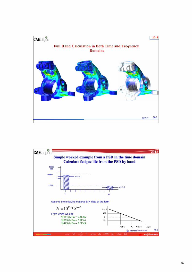
Number of upward zero crossings,
E[0] = 3
Number of peaks,
E[P] = 6
Irregularity factor,
= E[0]
E[P]= 3
6
Time History
x
xx
x
xx
x
γγ��
Zero and Peak Crossing Rates
RLD Ltd ©
2012
Dr NWM Bishop 355
Narrow band process
frequency Hz
0 5
2
2
0 5 10
0.5
1
Broad band process
frequency Hz
Time history PSD
0 5
5
5
0 5 10
0.5
1
Sine wave
frequency Hz
Time history PSD
0 5
0.5
0.5
0 5 10
∞�
White noise process
frequency Hz
0 5
10
10
0 5 10
1
2
0
0.1=γ
γ < 0.5
γ ≈ 0.5 to 0.95
0.1≈γ
Irregularity Factor

34
RLD Ltd 356 ©
2012
PSD statistics
RLD Ltd ©
2012
Dr NWM Bishop 357
Moments from a PSD
(Stress)2
Hz
Frequency, Hz
Gk(f)
fk
( ) ( )∑∫ ⋅⋅=⋅=∞
ffGfdffGfm nnn δ
0

35
RLD Ltd ©
2012
Dr NWM Bishop 358
Expected zeros, peaks and irregularity factor from a PSD
(Stress)2
Hz
Frequency, Hz
Gk(f)
fk
(� )� (� )�m f G f df f G f fnn n=� ⋅� =� ⋅� ⋅�
∞�
∫� ∑�0
δ�
0
2]0[mmE =
2
4][mmPE =
40
22
][]0[
mmm
PEE
==γ
RLD Ltd ©
2012
Dr NWM Bishop 359
Calculating fatigue life by hand in the frequency domain
Intensity given by rms =
Number of cycles given by E[P]
Distribution of cycles determined by irregularity factor number
if narrow band or Rainflow Cycle distribution (Dirlik – see later)
0m
36
RLD Ltd 360 ©
2012
Full Hand Calculation in Both Time and Frequency Domains
RLD Ltd ©
2012
Dr NWM Bishop 361
Assume the following material S-N data of the form
From which we get: N(141) MPa = 9.4E+5 N(315) MPa = 3.2E+4 N(423) MPa = 9.3E+3
Simple worked example from a PSD in the time domain Calculate fatigue life from the PSD by hand
101
2 500
10000
MPa2
Hz
df=1.0
df=1.0
Log S
Log N 9.4E+5
iS
iN9.3E+3
141
423
2.415 *10 −= SN

37
RLD Ltd ©
2012
Dr NWM Bishop 362
Assume process is made up from 2 sine waves
+
=
Range = 282MPa
Range = 141MPa
Range = 423MPa
RLD Ltd ©
2012
Dr NWM Bishop 363
Simple worked example from a PSD in the time domain
Sine wave 1 at 1 Hz with stress Sine wave 2 at 10 Hz with stress rangerange 10 000 * 1.41 * 2 = 2822 500 * 1.41 * 2 = 141
Sine wave 2 at 10 Hz with stress range 2 500 * 1.41 * 2 = 141 42
3 M
Pa
-250-200
-150-100
-500
50100
150200250
0 0.5 1 1.5 2 2.5 3
An approximate conventional Palmgren-Miner calculation on the time signal would give E[D] = 10 + 1
9.4E+5 9.3E+3 E[D] = 1.06E-5 + 1.07E-4 = 1.18E-4
This corresponds to a fatigue life of 8462 secs
n S N n/N
Little cycles 10/s 141 940,000 10/940000
Big cycles 1/s 423 9,300 1/9300
141 MPa
In 1 second
SUM = 0.000118 damage per second

38
RLD Ltd ©
2012
Dr NWM Bishop 364
A simple worked example from a PSD in the frequency domain
∑ dmn = fn G(f) f
mn = 1n * 10,000 * 1 + 10n * 2,500 *1
m0 = 12 500 m1 = 35 000 m2 = 260 000 m4 = 25 010 000
0.465
RMS = Mo = 112 MPa
Representative sine wave range= 112 * 1.41 * 2 = 315 MPa
N(315)MPa = 3.2E+4
P-Mdamage = E[D] per sec. = 9.8
3.2E+4
This corresponds to a fatigue life of 3265 secs.
= 4.6 zero crossings per second
= 9.8 peaksper second
0
2]0[mmE =
2
4][mmPE =
==][]0[
PEE
γ
RLD Ltd ©
2012
Dr NWM Bishop 365
Summary of results
By hand from regenerated time signal (a wide band calculation?) = 8462 secs
By hand from PSD directly (a narrow band calculation?) = 3265 secs
Computer based result (using MSC.Fatigue) (Narrow Band) = 1472 secs
Computer based result (using MSC.Fatigue) (Wide Band – Dirlik) = 7650secs

39
RLD Ltd 366 ©
2012
The Concept of Equivalent Stresses and Test Acceleration Techniques
RLD Ltd ©
2012
Dr NWM Bishop 367
Fatigue Damage for Random Response Histories
P - M damage ratio =
ni = p(S).dS.St= p(S).dS.E[P].T
St = total no. of cycles in required time = E[P].T
Stn iD = = Smp(S)dS N(Si) K ∫∫��∑∑��
i
∫∫�� Smp(S)dS D = E[P]T
K
N(Si) = K
Sm
p(S) is therefore the all important output
n iN(Si)
∑∑��i

40
RLD Ltd ©
2012
Dr NWM Bishop 368
( )S S p S dSeqm
m
=⎡
⎣⎢
⎤
⎦⎥
∞
∫0
1/
The Concept of “Equivalent Stress”
meqS
KTPEDE ⋅= ][][
( ) ⎥⎦
⎤⎢⎣
⎡= ∫
∞
dSSpSKTPEDE m
0
.][][
RLD Ltd 369 ©
2012
More on test acceleration methods

41
RLD Ltd 370 ©
2012
Rainflow cycle counts from PSDs
(and other methods that calculate fatigue damage directly)
RLD Ltd ©
2012
Dr NWM Bishop 371
Solution methods
Dirlik
Narrow Band
Tunna
Hancock Wirsching Chaudhury & Dover
Steinberg
The best method in all cases
Developed for offshore use
Railwayengineering(UK)
Electronic components (USA)
}}
The original solution
42
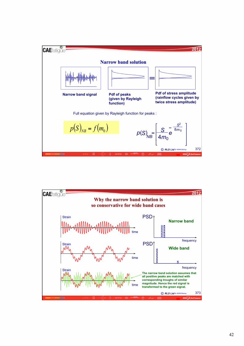
RLD Ltd ©
2012
Dr NWM Bishop 372
Narrow band solution
Narrow band signal Pdf of peaks (given by Rayleigh function)
Pdf of stress amplitude (rainflow cycles given by twice stress amplitude)
Full equation given by Rayleigh function for peaks :
⎣� ⎦�
p SNB
( ) =�⎡�⎢�⎢�
⎤�⎥�⎥�
S em4 0
Sm�� 8
2
0( ) ( )0mfSp NB =
RLD Ltd ©
2012
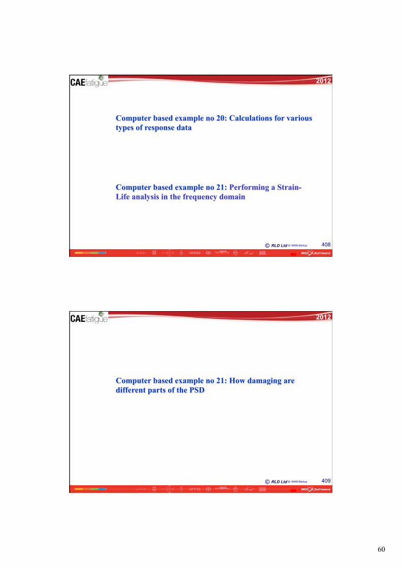
Dr NWM Bishop 373
Why the narrow band solution is so conservative for wide band cases
time
time
time
frequency
frequency
Narrow band
Wide band
The narrow band solution assumes that all positive peaks are matched with corresponding troughs of similar magnitude. Hence the red signal is transformed to the green signal.
PSD
PSD
Strain
Strain
Strain

43
RLD Ltd ©
2012
Dr NWM Bishop 374
Steinberg Solution “Three Banded Technique”
Used for testing electronic equipment in the USA. Based on the assumption that stress levels occur for
68.3% time at 1rms, 27.1% time at 2rms, 4.3% time at 3rms
( )0mfS Steineq =
( ) ( ) ( ) mmmm
Steineq mmmS1
000 6043.04271.02683.0 ⎥⎦⎤
⎢⎣⎡ ⋅⋅+⋅⋅+⋅⋅=
RLD Ltd ©
2012
Dr NWM Bishop 375
Dirlik solution
P(S
)
S
Stre
ss (M
Pa)
Time (secs)
Parameter fitting
M0M1M2M4
PSD1 TS1 RCC1 PDF1 Moms1 v PDF1
PSD2 TS2 RCC2 PDF2 Moms1 v PDF2
PSD3 TS3 RCC3 PDF3 Moms3 v PDF3
. . . . . v .
PSDi TSi RCCi PDFi Momsi v PDFi
PSD65 TS65 RCC65 PDF65 Moms65 v PDF65

44
RLD Ltd ©
2012
Dr NWM Bishop 376
Dirlik Solution
A widely applicable solution developed after extensive Monte Carlo simulation of a wide range of likely stress response conditions
( ) ( )4210 ,,, mmmmfSp D =
( )p S
DQ
e D ZR
e D Ze
mD
ZQ
ZR
Z
( ) /=+ +
− − −1 2
22
32
01 2
2
2
2
2
( )( ) ( )
( )( )
where; =m
m
D
2
0
3
Z Sm m
x mm
mm
Dx
DD DR
D D QD D RD
R x DD D
mm
m
= =⎡
⎣⎢
⎤
⎦⎥ =
−
+=
− − +
−
= − − =− −
=− −
− − +
2
21
11
1125
1
01 2
4
1
0
2
4
1 2
1
2
2 21 1
2
1 23 2
1
12
1 12
/
/
.
γγ
γ
γ
γ γγ
RLD Ltd ©
2012
Dr NWM Bishop 377
Dirlik solution
0
0.2
0.4
0.6
0.8
1
1.2
0 0.5 1 1.5 2 2.5 3 3.5 4Z=rms/2
p(S)
Part1Part2Part3total

45
RLD Ltd ©
2012
Dr NWM Bishop 378
Dirlik solution
0
0.5
1
1.5
2
2.5
3
3.5
4
5.31
26.6
47.8 69
90.3
112
133
154
175
197
218
239
260
281
303
324
345
366
388
409
430
451
473
494
515
536
558
rms
cycl
es
total
For an E[P] of 51.929 and dS=10.622 -> (Z=dS/(2*rms)
RLD Ltd ©
2012
Dr NWM Bishop 379
p S Sm
eT
Sm( ) =
⎡
⎣
⎢⎢
⎤
⎦
⎥⎥
−
4 20
8
2
20
γγ
Tunna solution

46
RLD Ltd ©
2012
Dr NWM Bishop 380
Wirsching solution
[ ]E D E D a m a mWirsch NBc m[ ] [ ] . ( ) [ ( )]( ) ( )= + − −1 1 ε
where;a(m)=0.926-0.033m ; c(m)=1.587m-2.323;
m, in this case, is the slope of the S-N curve
ε γ= −1 2
RLD Ltd ©
2012
Dr NWM Bishop 381
Chaudury and Dover solution
( )S mm m
erfm
eq C D
m m
&
/
( )=+⎛
⎝⎜
⎞⎠⎟ +
+⎛⎝⎜
⎞⎠⎟ +
+⎛⎝⎜
⎞⎠⎟
⎡
⎣⎢
⎤
⎦⎥
+
2 22
12 2
22 2
220
2 1ε
π
γγγ
Γ Γ Γ
where; erf(γ) = 0.3012γ + 0.4916γ2 + 0.9181 γ3 - 2.3534 γ4 - 3.3307 γ5 + 15.6524 γ6 - 10.7846 γ7
Again, m is the slope of the S-N curve
⎟⎠
⎞⎜⎝
⎛ +Γ
21m Is a Gamma function (tabular function used to
avoid numerical integration)
Hancock solution
( )S mm
eq Hanc
m
= +⎛⎝⎜
⎞⎠⎟
⎡
⎣⎢
⎤
⎦⎥2 2
210
1
γ Γ/

47
RLD Ltd ©
2012
Dr NWM Bishop 382
A new rainflow range definition (by Ryclik)
point 2
point 4
- ve time + ve
point 5 point 1 point 3
S (= h intervals)
( ),1 hipip −Υ
( ),2 hipip −Υ
( ),3 hipip −Υ
Level ip
RLD Ltd ©
2012
Dr NWM Bishop 383
A new rainflow range definition (by Bishop)
( ) ( ) ( ) ( )p SdS
ip ip h ip ip h ip ip hip h
ip nts
( ) . , , ,= − − −= +
= −
∑2 0
12
1
Υ Υ Υ p ip2 3
( ),1 hipip −ΥWhere is the probability of transitioning from a level below (ip-h) to level ip

48
RLD Ltd ©
2012
Dr NWM Bishop 384
The Kowalewski joint distribution between adjacent peaks and troughs
RLD Ltd ©
2012
Dr NWM Bishop 385
Examples: Computer Based Ford Intercooler Fatigue Analysis

49
RLD Ltd ©
2012
Dr NWM Bishop 386
The problem - a 3D loading plot
1100
1850
2600
3350
4100
0
20
40
0100
200300
400500
600
Measured R
PM
Frequency Range (Hz)
Acc
eler
atio
n R
ms-
AM
P (m
/s2 )
RLD Ltd ©
2012
Dr NWM Bishop 387
Waterfall plot of measured inter-cooler response
rpm 1100 - 4700 frequency 0 - 300Hz
Frequency [Hz] 0 300
Rev
s pe
r min
ute
(rpm
)
1100
4700

50
RLD Ltd ©
2012
Dr NWM Bishop 388 RLD Ltd© Dr NWM Bishop 388
1100
1600
2100
2600
3100
3600
4100
4600
0
50
100
150
200
250
0 50 100 150 200 250 300
Waterfall plot of NASTRAN generated rms response
rpm 1100 - 4700 frequency 0 - 300Hz
Frequency (Hz)
rms
acce
l (m
/sec
^2)
Revs per m
inute (rpm)
RLD Ltd ©
2012
Dr NWM Bishop 389
Stress PSD estimated using NASTRAN
1 26 51 76 101 126 151 176 201 226 251S1
S11
S21
S31
S41
S51S61
S71
0
100
200
300
400
500
pow
er
frequency
Fatigue damage at each rpm
0
0.2
0.4
0.6
0.8
1
1.2
1.4
1100
1600
2100
2600
3100
3600
4100
4600
4700
4000
3500
3000
2500
2000
1500
1100
0 50 100 150 200 250 300
speed

51
RLD Ltd ©
2012
Dr NWM Bishop 390
Combining FEA Stress Output with Customer Usage Factors
Fatigue damage at each rpm
0
0.2
0.4
0.6
0.8
1
1.2
1.4
1100
1300
1500
1700
1900
2100
2300
2500
2700
2900
3100
3300
3500
3700
3900
4100
4300
4500
4700
Arbitrary usage factor
0
0.005
0.01
0.015
0.02
0.025
0.03
0.035
Resultant fatigue damage
0
0.0005
0.001
0.0015
0.002
0.0025
RLD Ltd ©
2012
Dr NWM Bishop 391
Comparison of Time Domain with Frequency Domain
Time Domain
Assumptions about Loading None
Assumptions about structure Usually linear (not always)
Benefits/disadvantages Quite time consuming Not so informative Can work for non-linear
Frequency Domain
Assumptions about Loading Gaussian Stationary Random
Assumptions about structure Linear
Benefits/disadvantages Fast Efficient Informative

52
RLD Ltd ©
2012
Dr NWM Bishop 392
Beware of file sizes
100 input load
100,000 output nodes
100 frequencies
(12 pieces of stress info for each node)
Results in 1.2E10 bits of information being generated
RLD Ltd 393 ©
2012
Spectral Fatigue Damage Editing

53
RLD Ltd ©
2012
Dr NWM Bishop 394
Spectral Fatigue Damage Editing - system (fatigue analysis)
Original Stress Response
5th peak reduced by 50% 5th peak reduced
by 100%
Fatigue life = 34 hours
Fatigue life = 123 hours
Fatigue life = 58 hours
RLD Ltd 395 ©
2012
Spectral Fatigue Damage Editing

54
RLD Ltd ©
2012
Dr NWM Bishop 396
Questions and Summing Up Session
RLD Ltd ©
2012
Dr NWM Bishop 397
Gaussian (normal) table
3.00 rms

55
RLD Ltd ©
2012
Dr NWM Bishop 398
Some random vibration tests comprise of a sine wave input to the test structure that varies with time. In order to recreate the same environment within a computer analyses it would be necessary to perform a time based transient analysis. However, by making some approximations it is possible to perform such an analysis using frequency domain methods
1. Calculate, for each sine wave, an equivalent rms (0.707 * amplitude).
2. Square this value to get the area of an equivalent strip in a (peak hold) PSD.
3. Assume a PSD interval width of, say 1Hz, and this then defines the PSD height.
4. Repeat for all frequencies of interest.
5. For each frequency of interest perform a frequency response analysis with Nastran using a Tabled1 value of 1.0 over the entire frequency range.
6. Run MSC.Fatigue vibration and get the (peak hold) output PSD of stress caused by the input (peak hold) PSD.
7. Using a suitable pcl macro, read the value of each frequency component from [6] and (assuming a 1Hz interval width as above) calculate an equivalent sine wave response (reverse of steps [1] & [2]).
8. Run mclf or mslf to calculate the number of allowable cycles for each sine wave (set “constant range” and “constant mean” in order to bypass the rainflow counting process).
9. Take the reciprocal of [8] and factor by the time spent at each frequency. This information will come from the sweep rate.
10. Add together the damages to get the total damage/fatigue life
Dealing with sine sweep test simulations using MSC.Fatigue
RLD Ltd ©
2012
Dr NWM Bishop 399
Computer based example no 11: The variation of fatigue life with sample length Run mSLF to vary the duration of the sample used to calculate fatigue life. Estimate the possible error in the calculation for a particular sample length.
Start with Pave1.dac. This file is acceleration v time
Pick a material S-N curve using PFMAT. Find the stress that gives N=100,000
Use mART to scale up and transform units into MPa v time (rename the file)
Run mSLF and do a fatigue calculation on the whole of the stress v time signal
Repeat the calculation using 1st half then 2nd half of sample.
Repeat the calculation using 1st quarter etc.

56
RLD Ltd ©
2012
Dr NWM Bishop 400
Computer based example no 12: Using Nastran to generate transfer functions (frequency response functions)
RLD Ltd ©
2012
Dr NWM Bishop 401
Computer based example no 13: Count how many bigcycles go to 3 rms peak heights

57
RLD Ltd ©
2012
Dr NWM Bishop 402
Computer based example no 14: Calculating PSD’s From Time Signals Use mASD to calculate a PSD from WEG01.dac. Experiment with the buffer size and window size.
What happens to the scatter in the PSD as the buffer size goes down?
What happens to the number of points in the PSD as the buffer size goes down?
RLD Ltd ©
2012
Dr NWM Bishop 403
Computer based example no 15: Calculating Cross PSD s From Time Signals Use mFRA to calculate the cross PSD between track_horiz_right.dac and track_vert_right.dac.
Try the same calculation between weg01.dac and weg02.dac.
Discuss the issue of correlation!

58
RLD Ltd ©
2012
Dr NWM Bishop 404
Computer based example no 16: Calculating amplitude probability density functions.
Use mADA to calculate the amplitude probability density function and amplitude distribution function for weg01.dac
RLD Ltd ©
2012
Dr NWM Bishop 405
Computer based example no 17: Calculating running statistics Use mRSTATS to calculate the statistics of blocks of data along the time signal weg01.dac

59
RLD Ltd ©
2012
Dr NWM Bishop 406
Computer based example no 18: Using mFLF
• Start with wegxx.dac
• Calculate fatigue life (use mSLF) from time signal (pick a suitable S-N curve)
• Calculate the PSD from the time signal (use mASD)
• Then calculate the fatigue life from the PSD (use mFLF)
• Compare the fatigue life, E[P], E[0] etc.
• Compare the rainflow cycle distributions (use mCDA)
RLD Ltd ©
2012
Dr NWM Bishop 407
Computer based example no 19: Comparing the available methods
60
RLD Ltd ©
2012
Dr NWM Bishop 408
Computer based example no 20: Calculations for various types of response data
Computer based example no 21: Performing a Strain-Life analysis in the frequency domain
RLD Ltd ©
2012
Dr NWM Bishop 409
Computer based example no 21: How damaging are different parts of the PSD