2012-2013 { master 2 { macro i lecture 3 : the ramsey ... · pdf file2012-2013 { master 2 {...

2012-2013 – Master 2 – Macro I

Lecture 3 : The Ramsey Growth Model

Franck Portier(based on Gilles Saint-Paul lecture notes)

[email protected]

Toulouse School of Economics

Version 1.107/10/2012

Changes from version 1.0 are in red

1 / 42

[email protected]

Disclaimer

These are the slides I am using in class. They are notself-contained, do not always constitute original material and docontain some “cut and paste” pieces from various sources that Iam not always explicitly referring to (not on purpose but because ittakes time). Therefore, they are not intended to be used outside ofthe course or to be distributed. Thank you for signalling me typosor mistakes at [email protected].

2 / 42

mailto:[email protected]

0. Introduction

I The Ramsey model is a model of optimal growth for a closed,neo-classical economy populated by a representativeconsumer. While the Solow model assumes a fixed savingsrate, in the Ramsey model the savings behaviour comes fromthe intertemporal optimization by consumers.

I Strictly speaking, the Ramsey model is a normative model : ittells us what the optimal growth path is.

I However, it can be interpreted as a positive model of how theeconomy actually evolves.

I The reason is that if markets are complete and competition isperfect, any Walrasian equilibrium must be Pareto-optimal.But if there is a single representative agent, there is a uniquePareto-optimum : the one that maximizes the utility of therepresentative agent. Therefore, the optimal path of theRamsey model is also an equilibrium ; one under thoseassumptions.

3 / 42

1. The ModelFundamentals

I There is a representative consumer whose utility is

V =

∫ +∞

0e−ρt

Cαt − 1

αdt.

ρ is the rate of time preference and α ∈ (−∞, 1] the exponentparameter in the utility function. The intertemporal elasticityof substitution is then equal to

σ = 1/(1− α).

I The production function is

Yt = F (Kt ,AtLt). (PF)

Kt is the capital stock, Lt is total employment, and At anexogenous trend of labor-augmenting technical progress.

4 / 42

1. The ModelFundamentals (continued)

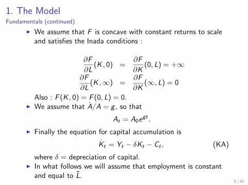
I We assume that F is concave with constant returns to scaleand satisfies the Inada conditions :

∂F

∂L(K , 0) =

∂F

∂K(0, L) = +∞

∂F

∂L(K ,∞) =

∂F

∂K(∞, L) = 0

Also : F (K , 0) = F (0, L) = 0.I We assume that A/A = g , so that

At = A0egt .

I Finally the equation for capital accumulation is

Kt = Yt − δKt − Ct , (KA)

where δ = depreciation of capital.I In what follows we will assume that employment is constant

and equal to L.5 / 42

1. The ModelExercise

I Exercise : Let F (K ,AL) = F (K ,AL)− δK be the net GDPproduction function. Does it satisfy the Inada conditions ?How would the model be rewritten if net GDP Y = Y − δKwere used instead of gross GDP ?

6 / 42

2. Solving the modelFOC

II To solve the model we apply the optimal control technique.The Hamiltonian is

Ht = e−ρtCαt − 1

α+ λt [F (Kt ,AtLt)− δKt − Ct ] .

I The optimality conditions are

∂H

∂C= 0⇐⇒ e−ρtCα−1

t = λt .

I This means that the marginal utility of consumption is equalto the marginal benefit of its alternative use, i.e. the value ofone unit of capital.

∂H

∂K= −λ⇐⇒ λ

(∂F

∂K− δ)

= −λ.

7 / 42

2. Solving the modelCo-state variable

I Since λ is also equal to the marginal value of consumption,this means that

λt =

∫ +∞

te−ρvCα−1

v

(∂F

∂K− δ)

dv .

I Therefore, λt is the net value of the future flow of marginalproducts of capital, net of depreciation, expressed in utilityterms.This is indeed what I would get if God gave me an extraunit of capital for free at date t.

I We can introduce µt , the contemporaneous co-state variable,such that λt = µte

−ρt . We get

Cα−1t = µt (1)

and

µt

(∂F

∂K(Kt ,AtLt)− δ

)= −µt + ρµt . (2)

8 / 42

2. Solving the modelA digression on asset values

I Consider an asset which pays a dividend dt and whose valueat t is Vt . Assume that I can get a rate of return elsewhereequal to r . This implies that the flow of dividends will bediscounted at rate r .

I To see this, note that if I sell my asset now and invest theproceeds at rate r , I will get (1 + r)Vt tomorrow. If I hold it, Iwill get dt + Vt+1. Therefore the arbitrage condition is

Vt =dt + Vt+1

1 + r. (3)

I Equivalently we can write :

rVt = dt + (Vt+1 − Vt). (4)

9 / 42

2. Solving the modelA digression on asset values (continued)

I That is :

Rate of Return x Value of the asset = Dividends + CapitalGains.

I This means that the rate of return on the asset must beequal to the rate of return on the alternative investment,otherwise there would be arbitrage possibilities.

I Note that for risk neutral agents, the formula extends to riskyinvestments :

rVt = dt + Et(Vt+1 − Vt).

I That is :

Rate of Return x Value of the asset = Dividends + ExpectedCapital Gains

10 / 42


I An equation like (3) can be solved by forward integration

Vt =1

1 + r

T∑i=t

1

(1 + r)i−tdi +

VT+1

(1 + r)T+1−t . (5)

I Assume that the following sequence :

Ft =1

1 + r

+∞∑i=t

1

(1 + r)i−tdi (6)

exists. Then if r > 0 Ft is the only non explosive solution to(5). So, if we eliminate explosive solutions, then we have aunique one which is called the fundamental value of the asset.

I Furthermore, let Vt be any other solution. Let Bt = Vt − Ft .It must be that

Bt+1 = (1 + r)Bt .

I Therefore, any solution is the sum of the ”fundamental” and a”bubble” which explodes at rate r .

11 / 42


I Remark : In fact the bubble can be stochastic and only needto explode at rate r in expectations. That is, up to amultiplicative factor (1 + r) the bubble can be any martingale.

I Remark : Conversely, any present discounted value of anincome flow can be rewrittenn in a recursive fashion. Forexample if

Wt =+∞∑i=t

1

(1 + r)i−tyi , (7)

one can always express Wt as a function of the income streamtoday and tomorrow’s value Wt+1 :

Wt = yt +1

1 + rWt+1. (8)

Then this can be again interpreted in a dividend plus capitalgains fashion :

rWt = (1 + r)yt + Wt+1 −Wt . (9)12 / 42


I Exercise : Why are (7),(8), and (9) not quite similar to (6),(3) and (4) ? What does it have to do with the timing ofdividend payments ?

13 / 42


I The preceding derivations can be made in continuous time.I Suppose an asset yields a flow of dividends per unit of time

equal to x(t).I Suppose I can get a return r per unit of time elsewhere.I Let V (t) be the value of the asset at t.I Suppose I sell it and invest in the market over a small time

interval dt.I Then at t + dt I will have V (t)(1 + r .dt).I If instead I hold the asset, then at t + dt I will have

x(t).dt + V (t + dt).I Hence

x(t).dt + V (t + dt) = V (t)(1 + r .dt),

I that is, neglecting second order terms :

rV (t) = x(t) + V (t)

14 / 42


rV (t) = x(t) + V (t)

I The LHS is the rate of return (per unit of time) times thevalue of the asset.

I The RHS is the dividend per unit of time, plus the expectedcapital gain per unit of time.

I The equation is the same as (4), except that the arbitragetakes place over a small time interval and that all is expressedper unit of time.

I In continuous time the fundamental is

Ft =

∫ +∞

te−r(v−t)x(v)dv

I And a bubble is such that

B = rB that is Bt = B0ert .

15 / 42


I Exercise : How are the above derivations altered when theinstantaneous discount rate is time-dependent ?

I RecallrVt = dt + (Vt+1 − Vt). (4)

rWt = (1 + r)yt + Wt+1 −Wt . (9)

I Exercise : Derive the continuous-time equivalent of (9) forWt =

∫ +∞t e−r(v−t)x(v)dv . Why is it that in continuous time

there is no longer a discrepancy like the one between (9) and(4) ?

16 / 42


I Throughout the course we will see that any dynamic equationwhich drives the evolution of a ”price” variable can beinterpreted as an arbitrage equation on an asset.

I This is true also for the marginal social values (=co-statevariables) in a dynamic optimization problem. For example,take (2).

µt

(∂F


)= −µt + ρµt . (2)

I We know that µt is the marginal value of an extra unit ofcapital at date t, expressed in utility terms and discounted atthe current date t.

I Also, the required rate of return in utility terms is ρ : To bewilling to sacrifice one unit of utility at t I need to get eρ(t′−t)

units of utility at a future date t ′.

17 / 42


µt

(∂F


)= −µt + ρµt . (2)

I So equation (2) can be rewritten

ρµt = xt + µt ,

wherext = µt

(∂F∂K (Kt ,AtLt)− δ

)= Cα−1

v

(∂F∂K (Kt ,AtLt)− δ

)I xt is the marginal utility of consumption times the net

marginal product of capital

I xt is the dividend in hedonic terms of one extra unit ofcapital, and µt is the capital gain.

18 / 42

2. Solving the modelThe transversality condition

I The transversality condition is

limt→+∞

λtKt = limt→+∞

e−ρtµtKt = 0.

19 / 42

2. Solving the modelThe Euler condition

I We can eliminate µt between (2) and (1) to get a dynamicrelationship between consumption and capital. We have that

µ

µ= − 1

σ

C

C

andµ

µ= ρ+ δ − ∂F

∂K(Kt ,AtLt).

I ThereforeC

C= σ(

∂F

∂K(Kt ,AtLt)− δ − ρ). (ec)

or

Growth rate of consumption

= Intertemporal elasticity of substitution x

(net marginal product of capital - rate of time preference).

I This is the standard condition that comes out ofpartial-equilibrium dynamic consumption problems. 20 / 42

2. Solving the modelRenormalization

I We know from previous lecture that there exists a balancedgrowth path with growth rate g .

I A standard trick is to renormalize the variables by dividingthem by the growth trend of productivity A.

I In a BGP the renormalized variables are therefore constant.

I For any variable Xt in the model let us define xt = Xt/At .

I Other renormalizations are possible provided they all deliverconstant renormalized variables in a BGP.

I Exercise : Based on what you know about a BGP, propose 3alternative renormalizations that have this property.

21 / 42

2. Solving the modelRenormalization

I Because of constant returns, we can rewrite F as

F (Kt ,AtLt) = AtLt f (Kt

AtLt).

I From the renormalization we get the following :

yt = Lf (kt

L), (pf)

kt = yt − (δ + g)kt − ct . (ka)

I Note also that∂F

∂K(Kt ,AtLt) = f ′(

kt

L)

I This allows us to derive the renormalized Euler condition :

ctct

= σ(f ′(kt

L)− δ − ρ)− g . (ec)

22 / 42

3. The balanced growth pathLong run capital stock

I In the BGP, renormalized variables are constant. Therefore,the BGP is characterized by the following condition :

f ′(kt

L)− δ = ρ+

g

σ. (MGR)

This pins down the capital stock in the long run.

I In words :

Net marginal product of capital

= rate of time preference + growth rate/intertemporal elasticity

of substitution.

23 / 42

3. The balanced growth pathLong run capital stock (continued)

f ′(kt

L)− δ = ρ+

g

σ. (MGR)

I Interpretation :I The greater ρ, the more people, prefer to consume now rather

than later. As a result they save less and accumulate lesscapital.

I The greater g , the more they must consume in the futurerelative to now, and therefore the greater the return on capitalnecessary to induce them to do so. Because of decreasingreturns to capital this means a lower level of capital relative tothe growth trend. (A difficulty here is that an increase in gaffects our normalization).

I Exercise : Can there be a balanced growth path if utility isnot a power function of consumption ?

24 / 42

3. The balanced growth pathThe Modified Golden Rule

I The problem with that kind of interpretation is that it tells uswhat must hold in equilibrium but it does not tell us by whateconomic mechanism that is achieved

I Assume growth accelerates. Holding the return to capitalconstant, people would want to borrow against the higherfuture income to consume more today. But in equilibrium thismust come at the expense of capital accumulation : weaccumulate less capital, this increases the return to capitaland makes us less averse to postponing consumption.

I In equilibrium we therefore has less capital and higherconsumption growth than before.

I The greater σ, the less sensitive to growth is the marginalproduct of capital. This is because if σ is large, only a smallincrease in that marginal product is required to induceconsumers to postpone consumption by enough in order tokeep up with the growth trend.

I (MGR) : modified golden rule or ”Keynes-Ramsey” condition. 25 / 42

4. Convergence to the balanced growth pathPhase diagram

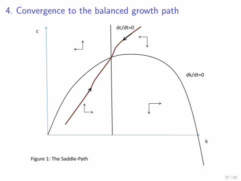
I A key result is that the economy converges to the balancedgrowth path.

I This is illustrated by a phase diagram (fig. 1).

I The c = 0 schedule corresponds to (ec), while the k = 0schedule comes from (ka), where y is replaced by Lf (kt

L).

I The arrows define the law of motion of the economy in the(k , c) space and come from those equations.

26 / 42

4. Convergence to the balanced growth path

dk/dt=0

dc/dt=0c

k

Figure 1: The Saddle-Path

27 / 42

4. Convergence to the balanced growth pathUniqueness

I At any date t the capital stock is determined from the past.

I In other words it cannot jump and must evolve smoothlyaccording to the differential equation (ka).

I On the other hand, at a given initial date consumption maybe anything.

I But thereafter it must also evolve smoothly according to (ec).Thus consumption cannot jump in a perfectly anticipated waybecause this would violate (ec). But its initial value is notpinned down by the past.

I In principle there is an infinity of possible trajectories, eachcorreponding to a choice for the initial consumption c .

28 / 42

4. Convergence to the balanced growth pathUniqueness (continued)

I However :I If initial consumption is too high, then the subsequent

trajectory implies that capital is exhausted in finite time. Thenconsumption hits its zero boundary and must remain equal tozero thereafter. Consequently, it is not differentiable at thedate when capital becomes equal to zero which violates (ec).These paths cannot be optimal.

I If initial consumption is too low, the subsequent trajectoryinvolves a normalized consumption which goes to zero. Pickinga slightly higher consumption level would yield higherconsumption at each date, which clearly dominates the initialtrajectory. Therefore the initial trajectory cannot be optimal.Technically, the condition which is violated is the transversalitycondition.

29 / 42

4. Convergence to the balanced growth pathProof of uniqueness

I Asymptotically we have, along such paths, that c = 0.I The asymptotic value of k is k such that Lf ( k

L) = (δ + g)k .

I By concavity, Lf (kL

) > kf ′(kL

).

I Thus f ′(kL

)< δ + g . Let z = δ + g− f ′

(kL

)> 0.

I Substituting into (2) we then get that

µt = (z + ρ− g)µt .

Hence :µt = µt0 exp((z + ρ− g)(t − t0)).

I Finally,

e−ρtµtKt = e−ρtµt0 exp((z + ρ− g)(t − t0))kAt

= e−ρtµt0 exp((z + ρ− g)(t − t0))kA0egt

= M.ezt →∞,where M is a constant.

30 / 42

4. Convergence to the balanced growth pathInterpretation of the proof

I At k the net marginal product of capital is lower than g .I This means that by reducing k I would lose less than the

fraction of GDP I need just to maintain k in line with thegrowth trend. This would free a surplus that I could consume.

I So I will only keep this capital if its marginal value is expectedto appreciate by enough to offset that negative effect.

I But then the marginal value of capital must explode at such arate that the transversality condition is violated, (meaningthat I am keeping too much capital in the long run)

I Thus we see that the only acceptable trajectory is the onewhich converges to the steady state in the (k , c) plane, i.e.the BGP of the economy. This allows to pin down the initialvalue of consumption.

I Consequently, not only does the BGP exist, but the economyconverges to this BGP for any initial value of K .

I Note : The trajectory which converges to the BGP is calledthe saddle path. 31 / 42

5. Location of the Modified Golden RuleOn the left of Golden Rule

I One can show that the modified golden rule of the capitalstock is always to the left of, i.e. smaller than, the maximumpoint of the k = 0 schedule.

I Note that this maximum is the one which maximizesc = y − (δ + g)k = Lf (kt

L)− (δ + g)k.

I The FOC is f ′(k/L) = δ + g . Let k∗ be the MGR capital leveland k be the one corresponding to the top of k = 0.

I Then k∗ < k if and only if :

ρ+g

σ> g ,

I or equivalently, since σ = 1/(1− α),

αg < ρ. (10)

32 / 42

5. Location of the Modified Golden RuleInterpretation

I Consider the utility of the consumer in a BGP. Up to aconstant, it is equal to∫ +∞

0

(c0egt)

α

α

e−ρtdt =

∫ +∞

0

cα0α

e(gα−ρ)tdt.

I Clearly, this exists iff (10) holds.

I The meaning of this is that if (10) is violated, the growthpotential of the economy is such that an infinite amount ofutility can be obtained because the contribution of futureconsumption to utility grows faster than the rate of timepreference.

33 / 42

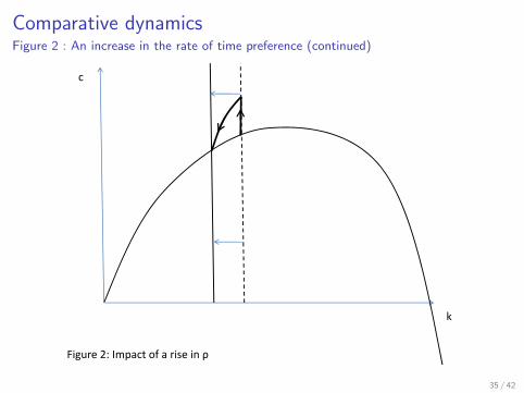
6. Comparative dynamicsAn increase in the rate of time preference.

II People are more impatient and start consuming more as thereturn to capital gets lower than their rate of time preference.

I As capital gets depleted, the economy becomes lessproductive and the MPK goes up.

I In equilibrium it has increased by the same amount as the rateof time preference and there is no longer an incentive todeplete it.

I The capital stock is lower and so must be consumption(otherwise we would be on a capital exhaustion trajectory).

34 / 42

Comparative dynamicsFigure 2 : An increase in the rate of time preference (continued)

c

k

Figure 2: Impact of a rise in ρ

35 / 42

6. Comparative dynamicsAn additive productivity shock (”manna from heaven”)

I Consumption jumps immediately by an amount equal to themanna.

I The manna is entirely consumed and the capital stock isunchanged.

I Starting from the initial capital stock, at the given rate ofreturn on capital consumers see an increase in their income bythe same amount in all current and future periods.

I Thus their current income and their permanent incomeincrease by the same amount.

I At this rate of return they thus want to increase theirconsumption permanently by that amount.

I As this leaves the capital stock unchanged, the rate of returnis unchanged and we indeed have an equilibrium outcome.

36 / 42

Comparative dynamicsFigure 3 : An additive productivity shock (”manna from heaven”) (continued)

c

k

Figure 3: Manna from heaven

37 / 42

6. Comparative dynamicsA multiplicative productivity shock

I Both schedules shift out.

I In the long term there is more capital and more consumption.This is because capital is more productive, so it is worthaccumulating more of it and use the proceeds to consumemore in the long-run.

I In the short run, the effect is ambiguous : there is asubstitution effect which tells us that it is worth consumingless today and more tomorrow because accumulating morecapital is now a better idea.

I There is an income effect which says that we will have moreincome throughout the whole trajectory and we may want toconsume a little bit more right now.

38 / 42

6. Comparative dynamicsFigure 4 : A multiplicative productivity shock (continued)

c

k

Figure 4: A multiplicative productivity shock

39 / 42

6. Comparative dynamicsAn anticipated manna from heaven

I At date t = 0 it is known that at some future date T theeconomy will undergo a permanent shock in one of theparameters.

I The key points here are thatI starting from T the economy must be on the new saddle pathI consumption cannot jump in perfectly anticipated fashion

because this would violate the optimality condition (ec)I Remark : By contrast, consumption may jump if there are

news, because when there are news people re-optimize. This iswhy consumption jumps upon the shock in all the precedingexamples, and will jump at t = 0 here).

I We see that between the announcement and the realization ofthe shock consumption goes up and the capital stock is beinggradually depleted.

I At the date of the shock we are exactly on the new saddlepath, so that consumption continues to grow but now we usethe manna to reaccumulate capital.

40 / 42

6. Comparative dynamicsAn anticipated manna from heaven (continued)

I Why is this optimal ? If we were waiting for the shock tomaterialize in order to consume more, consumption would notbe smooth.

I Relative to this, we can increase our utility by consumingmore now and less when the shock occurs.

I As a consequence, we have less capital at the time of theshock, but this raises its return above the rate of timepreference (adjusted for growth), so it makes sense togradually rebuild it.

41 / 42

6. Comparative dynamicsFigure 5 : An anticipated manna from heaven (continued)

c

k

Figure 5: Anticipated manna from heaven

42 / 42

2012-2013 { master 2 { macro i lecture 3 : the ramsey ... · pdf file2012-2013 { master 2 {...

Documents